Review: Sensing Technologies for the Optimisation and Improving Manufacturing of Fibre-Reinforced Polymeric Structures

Abstract

Over the last three decades, composite structures have become increasingly more common in everyday life, such as in wind turbines as part of the solution to produce clean energy, and their use in the aerospace industry due to their advantages over conventional materials. Most of these advantages are dependent upon the reliability and quality of the manufacturing process to ensure that there are no defects/faults or imperfections during manufacturing. Thus, it is critical to monitor the enclosed environment of moulds during fabrication in real time. This need has caused many researchers—past and present—to create or apply many sensing technologies to achieve real-time monitoring of the manufacturing processes of composite structures to ensure that the structures can meet their requirements. A consequence of these research activities is the myriad of sensing schemes, (for example, optical, electrical, piezo, and nanomaterial schemes and the use of digital twins) available to consider, and the investigations all of them have both strengths and weaknesses for a given application, with no apparent option having a distinct advantage. This review reveals that the best possible sensing solution depends upon a large set of parameters, the geometry of the composite structure, the required specification, and budget limits, to name a few. Furthermore, challenges remain for researchers trying to find solutions, such as a sensing scheme that can directly detect wrinkles/waviness during the laying-up procedure, real-time detection of the resin flow front throughout the mould, and the monitoring of the resin curing spatially, all at a spatial resolution of ~1 cm with the required sensitivity along with the need to obtain the true interpretation of the real-time data. This review offers signposts through the variety of sensing options, with their advantages and failings, to readers from the composite and sensing community to aid in making an informed decision on the possible sensing approaches to help them meet their composite structure’s desired function and tolerances, and the challenges that remain.

1. Introduction

Fibre-reinforced polymeric (FRP) materials are a class of composite materials made by combining a polymer matrix with reinforcing fibres. The polymer matrix, typically made from thermosetting plastics such as epoxy, vinyl ester, or polyester, acts as a binder that holds the fibres together and transfers loads between them, yielding strength and stiffness to the composite itself [1]. There are a variety of different materials used as the reinforcement, such as glass fibres (GFs), carbon fibres (CFs), aramid and basalt fibres, etc. [1,2,3]. The combination of the polymer matrix and reinforcing fibres results in a material that can outperform more conventional materials’ mechanical properties. The fibres provide high tensile strength and stiffness, while the polymer matrix offers toughness and resistance to environmental degradation. The combination of these properties yields a versatile material that can be tailored for specific applications by varying the type, orientation, and volume fraction of the fibres [4].

Over the last four decades, fibre-reinforced polymeric (FRP) structures have been playing an increasing role in engineering structures, with prime examples being in commercial aircrafts, where the FRP structures are replacing the metal structures in aerospace applications due to their high strength-to-weight ratio. They are used in the construction of aircraft components such as fuselage sections, wings, and tail assemblies, leading to improved fuel efficiency and performance [5,6,7]. Another important application is maritime wind turbines, using FRP materials to construct the blades, which can span in excess of 80 m for similar reasons [8,9,10]. Furthermore, there are important applications for FRP materials and structures in the construction industry for reinforcing concrete structures, such as bridges, buildings, and tunnels. FRP composites are preferred due to the previously mentioned advantages and their corrosion resistance [11,12]. The FRP composite structure’s corrosion resistance property is also exploited in the marine industry for building boat hulls, decks, and other structural components [13]. In addition, these FRP composites are commonly used in sports equipment due to their high strength, stiffness, and light weight, offering durability and greater manoeuvrability and control for sports such as tennis [14]. There are some recent advancements in the capabilities of FRP manufacturing, such as the use of smart carbon fibre-reinforced polymer composites that incorporate nanomaterials such as reduced graphene oxide (rGO) and carbon nanofibers (CNFs). These materials enhance the strain-sensing capabilities of the composites, allowing for more accurate damage detection and structural health monitoring [15].

Despite many benefits, FRP materials face some challenges. One of the main issues is the cost of the raw materials and manufacturing processes, which can be higher compared to traditional materials, along with their long-term durability and performance under various environmental conditions. These critical issues have been linked to improving quality control to ensure quality of the manufacturing process of the FRP composite structures themselves [16,17,18].

There are many processes to manufacture FRP composite structures [19,20,21,22,23,24,25,26,27,28]; these include manual hand laying-up [20], to the spray laying-up method (a manual procedure) [21], to more automated procedures, such as resin transfer moulding (RTM). Dry fibres are placed into a closed mould, and resin is injected under positive or negative pressure [22] and pultrusion beams and rods. Fibres are pulled through a resin bath and then through a heated die, which shapes and cures the resin [23]. Some of these procedures have been created for volume production of simple structures, like pultrusion [23] and compression sheet moulding (CSM) [25]. The authors refer to reader to review papers in Refs. [16,17,20] if the reader is unfamiliar with these processes. In closed-mould resin infusion processes, real-time monitoring is essential to produce reliable quality and the required performance from the FRP composite structure. There are inherent challenges to successfully monitor the closed mould by virtue of the fact that the mould is in a sealed environment. Therefore, a direct visual inspection of the resin’s progression is impossible, making it difficult to detect issues such as dry spots or voids. The moulds’ attributes of interest for real-time monitoring are flow front position, temperature, variations in the viscosity of the resin [29], cavity pressure, and curing. These yield real-time quantitative data on the status of the infusion, which allow the manufacturer to adjust process parameters to avoid defects.

With the exceptions of CSM and prepreg processing, in which the resin is already infused and partly cured, all the other manufacturing methods stated above can be simplified into three main stages: (i) locating and positioning the dry fibres, i.e., the laying-up process; (ii) the complete impregnation of the fibres inside the mould by the resin; (iii) the complete curing of the resin. All three stages are critical in creating FRP composite structures that have the desired physical attributes. Therefore, it is paramount that real-time monitoring of all three stages during manufacture occurs to ensure quality and minimise/eliminate defects, such as wrinkles or waviness, voids, dry patches, and insufficient curing [30]. This review focuses on practical and manual manufacturing approaches for FRP composites, with a particular emphasis on the sensing technologies used to monitor these processes. Special attention is given to resin and epoxy infusion methods for impregnating reinforcement fibres, highlighting the role of sensing technologies in enabling real-time monitoring, improving process efficiency, and ensuring consistent product quality.

These sensing or detection apparatuses help in detecting defects in the laying-up process, sensing the complete fibre impregnation and the monitoring of the curing process in real time to ensure the quality of the final product. These technologies are pivotal in optimising and improving the manufacturing processes, which ensures the structural integrity and longevity of FRP composites [31]. There are challenges with integrating sensing technologies, such as sensor compatibility with the FRP composite, and ensuring that the mechanical strength, along with other properties of the composite, is not compromised by the presence of the sensor or sensing array [32]. There are other issues that are being addressed by researchers at this present time, like the interpretation and understanding of real-time data from the sensors, along with creating algorithms and machine learning models to process and interpret the vast amount of data generated by the sensors [33,34]. Furthermore, these detection schemes tend to be relatively expensive to develop, produce, and deploy [35].

This review aims to give an overview of the present advancements in sensors and interrogation schemes that are being deployed to assist in the evaluation of the manufacturing process of FRP composite structures. There are several competing technologies and associated sensors being used and investigated by researchers at the present. The authors provide seven major classifications and additional sensing schemes that are on the fringes of researchers’ interest. This article looks at each sensing technology and the underlying mechanism used by the sensor for the monitoring, along with which stage of the manufacturing process they are to be used. Also, we make comparisons between the various schemes, and to each other where possible to give a clearer view of the sensors and associated sensing techniques advantages and limitations. During this review process, it has become apparent that there is no obvious option; they all have advantages and drawbacks—from the issues of interpretation for the integrated sensors, such as nanomaterial/piezoresistive types, to the spatial resolution of some distributed fibre optic sensing approaches. In addition, the advantages of nanomaterials creating a robust sensing network throughout the mould from the materials used to construct the FRP composite (see later sections). It should be noted that one of the primary applications of sensing technologies is in structural health monitoring, which is used during the operational lifetime of a product and, therefore, takes place after the manufacturing process [36,37]. While this application is beyond the scope of the current review, it will be referenced as a potential post-manufacturing benefit and area of application.

2. Sensors and Mechanisms

The sensors which are currently under investigation by researchers can be categorised into six classifications: optical, electrical, piezoelectric, imaging, nanomaterials, and ultrasonics [38,39]. At all three stages of the FRP composite fabrication process, sensors can be used. In general, the local environmental condition is monitored, such as temperature, pressure (stress or strain), chemical change (presence of a substance), and spatial location (positioning of fibres within a mould). In the following sections of this review, each classification of sensor and their associated interrogation scheme that are being investigated/utilised in FRP composites with respect to the specific stage of the manufacturing process will be considered.

2.1. Optical Sensors

This category is primarily based upon various types of optical fibres; this review does not explain the fundamental working principle of optical fibres, which is very much a subject in its own, but refers the reader to some references for a better understanding [40,41,42]. These fibre optical sensors can be subdivided into two types of sensors: discrete and distributed. The two types are based upon very different mechanisms. Their performances and limitations are studied, such as spatial resolution, cross-sensitivity, measurand accuracy, and time responsiveness, along with the stage of the manufacturing process within which it is being used. The main sensing schemes being used or investigated by researchers for the manufacturing processes are distributed Raman scattering temperature sensing and simulated Brillouin scattering for strain and temperature, known as quasi-distributed optical sensors [43,44,45,46].

2.1.1. Quasi-Distributed Optical Sensors

This group of sensors is widely used within composite materials [38] and can be divided into four basic types: fibre Bragg grating (FBG) sensor, FBG intra-cavity sensor, tilted fibre Bragg grating (TFBG) sensor, and long-period grating (LPG) sensors [47,48,49,50,51,52]. There has been a vast amount of work published on all types of grating sensors. A detailed analytical analysis is beyond the scope of the current study, but the reader will be signposted where to look for more information. All of these types of sensors have a periodic refractive index variation within the core that acts to couple light to the various modes of light that the optical fibre can support. There are many methods of fabrication for all three types of sensors. Some typical examples of fabrication technique are UV phase-mask inscription, UV point by point, direct-write femtosecond laser inscription, and the fusion-arc technique that can be used for the three types of sensors [53,54,55,56]. The core mode can be guided, lossy/leaky, and radiative [57,58]. The coupling to the different modes depends upon the type of grating performing the coupling along with the physical geometry and materials used to form the optical fibre.

Fibre Bragg Grating

These sensors have a radially symmetric refractive index perturbation away from the central axis of the optical fibre. Typically, the period of perturbation is approximately 1 μm in the core of the fibre (see Figure 1a), which leads to the majority of the light (forward propagating core mode) being coupled to back-reflected light (coupled into counter-propagating core mode) with a minority couple to the leaky and radiative modes [57,58] (see Figure 1b). This leaves a “notch” in the transmission spectrum of the illuminating light of the FBG sensor; see Figure 1c. A uniform FBG acts as a selective mirror in wavelength around the Bragg wavelength to yield a pass-band reflected spectrum, as depicted in Figure 1b. In fact, at each refractive index discontinuity along the fibre axis (see Figure 1a), a weak Fresnel reflection is generated. These weak reflections add in phase at the Bragg wavelength, yielding an important reflection band surrounded by side lobes.

An important attribute of FBGs is that they can have narrow spectral features in both transmission and reflection for good resolution and limit of detection (LOD); a typical spectral response is shown in Figure 2a. The disadvantage of using FBGs is their intrinsic insensitivity to the changes in the surrounding medium; this can be seen in the phase-matching condition for a FBG, which is given by the wavelength of resonant ${\lambda }_B=2n_{eff}\mathsf{\Lambda }$ and the maximum grating reflectivity $R={tanh}^2\left(\kappa L\right)$, where n_eff is the effective refractive index of the core mode, Λ is the period of the FBG, L is the length of the grating, and κ is the coupling coefficient. In the case of the sinusoidal uniform index perturbation Bragg grating, the coupling strength between the forward and backward modes can be described by a coupling coefficient: $\kappa =\left({\displaystyle \raisebox{1ex}{$\pi \delta n$}\!\left/ \!\raisebox{-1ex}{${\lambda }_B$}\right.}\right)\eta$. The variable $\delta n$ is the modulation of the refractive index of the grating; η represents the fraction of fibre mode power contained by the fibre’s core and it can be estimated using the normalised parameter V. On the basis that the grating is uniform, η can be approximated by $\eta \approx 1-V^{-2}$, and, using $V=\left({\displaystyle \raisebox{1ex}{$2\pi a$}\!\left/ \!\raisebox{-1ex}{${\lambda }_0$}\right.}\right)\sqrt{{n_{core}}^2-{n_{cladding}}^2}$, a is the core radius. n_core is the core refractive index. n_cladding is the cladding refractive index and λ₀ is the wavelength of the light in free space. The wavelength ${\lambda }_B$ is a function of ${\lambda }_B(\lambda ,\epsilon ,T,S_f)$ with the phase condition $2n_{eff}\mathsf{\Lambda }$, which should be written as ${\lambda }_B=2n_{eff}\left(\lambda ,\epsilon ,T,S_f\right)\mathsf{\Lambda }\left(\epsilon ,T\right)$. The variables are wavelength (λ) strain (ε), temperature (T), and S_f, which is the waveguide geometry and material factor [48]. Therefore, the use of FBGs as a sensor is dependent upon effecting one of these variables. The general strain sensitivity of a conventional FBG written in a single mode fibre (SMF) (step-index) optical fibre is 1.2 pm/με, and its temperature sensitivity is 11.5 pm/°C [48].

Fibre Bragg Sensors Mechanism for Strain and Temperature

The effective refractive index of the core and the spatial periodicity of the grating are both affected by changes in strain and temperature. In particular, the effective refractive index is modified through the thermo-optic and strain-optic effects, respectively. Hence, the Bragg wavelength shift Δλ_B due to strain Δε and temperature ΔT variations is given by the following:

$$\Delta {\lambda }_B=2\left(\mathsf{\Lambda }{\displaystyle \frac{d{n}_{eff}}{dT}}+n_{eff}{\displaystyle \frac{d\mathsf{\Lambda }}{dT}}\right)\Delta T+2\left(\mathsf{\Lambda }{\displaystyle \frac{d{n}_{eff}}{d\epsilon }}+n_{eff}{\displaystyle \frac{d\mathsf{\Lambda }}{d\epsilon }}\right)\Delta \epsilon$$

(1)

The first term in Equation (1) represents the effect of temperature on the Bragg wavelength. The Bragg wavelength shift due to thermal expansion comes from the modification of the grating spacing and the refractive index. The relative wavelength shift due to a temperature change ΔT can be written as

$${\displaystyle \frac{\Delta {\lambda }_B}{\Delta T}}={\lambda }_B\left({\displaystyle \frac{1}{n_{eff}}}{\displaystyle \frac{d{n}_{eff}}{dT}}+{\displaystyle \frac{1}{\mathsf{\Lambda }}}{\displaystyle \frac{d\mathsf{\Lambda }}{dT}}\right)$$

(2)

where ${\displaystyle \frac{1}{n_{eff}}}{\displaystyle \frac{d{n}_{eff}}{dT}}$ is the thermo-optic coefficient, which is approximately equal to 8.6 × 10⁻⁶ K⁻¹ for germanium doped silica core optical fibre; ${\displaystyle \frac{1}{\Lambda }}{\displaystyle \frac{d\Lambda }{dT}}$is the thermal expansion coefficient of the optical fiber, which is approximately equal to 0.55 × 10⁻⁶ K⁻¹ for silica, therefore the refractive index change is the dominant effect [59]. The order of magnitude of the temperature sensitivity of the Bragg wavelength is 10–12 pm/°C at an approximate wavelength of 1550 nm.

The second term in Equation (1) represents the effect of longitudinal strain on an optical fibre. It corresponds to a change in the grating periodicity, and the strain-optic effect induces a change in the refractive index [60]. Assuming that the grating is strained in the z-direction only and that the fibre material follows Hooke’s law, the Bragg wavelength shift as a result of the applied strain is defined by the following:

$$\Delta {\lambda }_B={\lambda }_B\left(1-p_e\right)\Delta \epsilon$$

(3)

$$p_e={\displaystyle \frac{n_{eff}^2}{2}}\left[p_{12}-\nu \left(p_{11}+p_{12}\right)\right]$$

(4)

The substitution of parameters (p₁₁ = 0.113, p₁₂ = 0.252, ν = 0.16 (Poisson’s ratio) and n_eff = 1.482 [39,40,41]) in Equations (3) and (4) gives a strain-optic constant p_e = 0.21 and an axial strain sensitivity of the Bragg wavelength of 1.2 pm/με at a wavelength of 1550 nm. The general case for strain is more complicated than for axial strain [61,62,63]; the strain-optic constant becomes a strain-optic matrix (Equation (5)):

$${\left({\displaystyle \frac{\Delta {\lambda }_B}{{\lambda }_B}}\right)}_i={\displaystyle \frac{\Delta \mathsf{\Lambda }}{\mathsf{\Lambda }}}+{\displaystyle \frac{\Delta n}{n}}={\epsilon }_l-{\displaystyle \frac{n_{eff}^2}{2}}\sum _{j=1}^3{p}_{ij}{\epsilon }_i$$

(5)

p_ij is the generic element of the stain-optic matrix, differing for each Cartesian axis, where i = 2, 3 is the polarisation axis of the light propagating along the optic fibre. Thus, the interpretation of the wavelength shifts Δλ_B of the FBG becomes a major task.

Tilted Fibre Bragg Sensors

In the case of the TFBG, the refractive index perturbation in the core is radially asymmetric from the central axis of the fibre; see Figure 2a. This index asymmetry of the core increases the coupling of the light to the leaky and radiative modes of the optical fibre [59] that have a greater dependence on the interface between the optical fibre and the surrounding medium thus, the refractive index of the surrounding medium (chemical). The TFBG is observed in its transmission spectra; an example spectra is shown in Figure 2b. Inspecting Figure 2b, the S₁ spectral feature is the resonant Bragg wavelength that was discussed previously, and the S₂ spectral feature are the coupling to the leaky and radiative modes of the optical fibre, causing resonances to occur. Furthermore, it is these S₂ spectral features that interact with the surrounding medium and the measurands already mentioned, whilst S₁ has only temperature and strain dependency.

Tilted Fibre Bragg Sensors Mechanism for Strain, Temperature, and Refractive Index (Chemical)

There are two major components in the transmission spectra of a TFBG. At the longer wavelength is the core mode Bragg wavelength phase matching condition, and on the short wavelength are cladding mode resonance wavelengths (Figure 2b). The Bragg wavelength can be expressed as ${\lambda }_B=\left(n_{effcore}+n_{effcore}\right)\mathsf{\Lambda }$, where each n_effcore represents the forward propagating core mode and counter-propagating core mode. The tilt angle of grating plane is with respect to the fibre axis; the grating period along the fibre axis could be modified as ${\Lambda }_g={\displaystyle \raisebox{1ex}{$\Lambda $}\!\left/ \!\raisebox{-1ex}{$\mathit{cos}\xi $}\right.}$. $\xi$ represents the tilt angle defined as the angle from the perpendicular section of the optical fibre. Thus, the Bragg wavelength condition is $\left(n_{effcore}\left(\lambda ,\epsilon ,T,S_f\right)+n_{effcore}\left(\lambda ,\epsilon ,T,S_f\right)\right){\displaystyle \raisebox{1ex}{$\Lambda $}\!\left/ \!\raisebox{-1ex}{$\mathit{cos}\xi $}\right.}$, and the resonance wavelength of cladding mode is determined by

$$\left(n_{effcore}\left(\lambda ,\epsilon ,T,S_f\right)+{n^{\nu }}_{effcladding}\left(\lambda ,\epsilon ,T,S_f,n_s\right)\right){\displaystyle \raisebox{1ex}{$\mathsf{\Lambda }$}\!\left/ \!\raisebox{-1ex}{$\cos \xi $}\right.}$$

(6)

where ${n^{\nu }}_{effcladding}$ is the effective refractive index of the $\nu$^th cladding mode [57]. Therefore, the cladding mode is affected by the surrounding medium because the waveguide interface that supports the cladding mode is the cladding material and the refractive index of the surrounding medium.

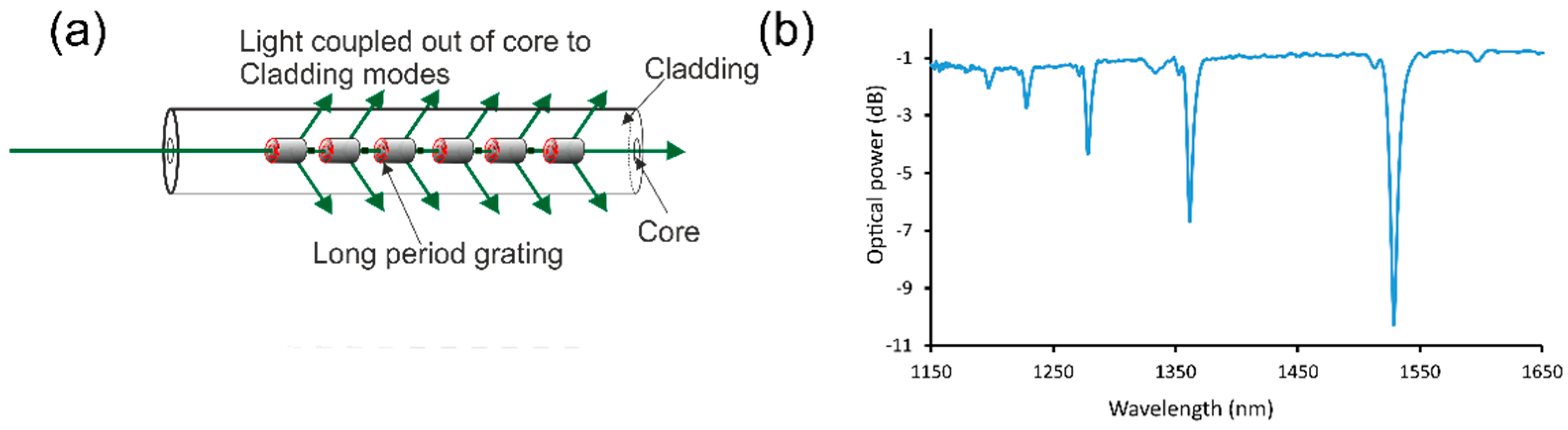
Long-Period Grating Sensors

The FBG sensor can be considered as a resonator with the light reflected within the core of the optical fibre. The LPG can be thought of as a dispersive element, that is, coupling light out of the core into the cladding (the outer glass section) of the optical fibre. Furthermore, the cladding can also be thought as a waveguide that supports many cladding modes; thus, when the core light is dispersed into the cladding for the given phase-matched conditions at various wavelengths and period of the LPG light can be coupled into cladding modes [59,64], resulting in a series of attenuation bands centred at a given wavelength λ_i in the transmission spectrum in the core of the optical fibre. Once this coupling has occurred, the light decays due to scattering losses, leaving these attenuation bands; see Figure 3. The LPG refractive index modulation in the optical fibre core has a typical perturbation of ~10⁻⁴ and periods between 100–600 μm. There are various methods and mechanisms to create the index modulation, like photoinduction (ultraviolet, 244 nm, point by point), structural material change (fusion-arc, point by point), and Femtosecond laser inscription (fissure/void creation) [55,57,59].

Fibre Long-Period Sensors Mechanism for Strain, Temperature, and Refractive Index Chemical

The centre wavelength λ_ν of an attenuation band is specified by the phase-matching conditions ${\lambda }_{\nu }=\delta n_{{eff}_{\nu }}\mathsf{\Lambda }$ where

$$\delta n_{{eff}_{\nu }}=n_{effcore}\left(\lambda ,\epsilon ,T,S_f,n_i\right)-{n^{1\nu }}_{effcladding}\left(\lambda ,\epsilon ,T,S_f,n_s,n_i\right)$$

(7)

${n^{1\nu }}_{effcladding}$ is the effective index of the ν^th radial cladding mode, and $n_{effcore}$ is the effective index of the core mode. Both are dependent on the indices (materials) of the various fibre layers, n_i, along with fibre geometry and the wavelength λ. Also, ${n^{1\nu }}_{Cl}$ is a function of the refractive index of the surrounding medium, n_s. Λ is the period of the LPG, T is the temperature, and ε is the strain experienced by the fibre. The quantity $\delta n_{{eff}_{\nu }}$ is the differential effective index between the core and cladding modes. In Equation (7), the superscripts denote the LP₀₁ core mode and the HE_1ν axially symmetric cladding modes: from this point forward, for brevity, we replace 1,ν with ν. We are assuming here that the grating consists of a circularly symmetric index perturbation transverse to the axis of the fibre, so that the only non-zero coupling coefficients between the core mode and the cladding modes involve cladding modes of azimuthal order 1 [63]. This creates a series of attenuation bands in the transmission spectra of the LPG (Figure 2b). Again, like the TFBG, the cladding modes have spectral sensitivity to the surrounding medium, but, here, the sensitivity can be significantly higher. The relationships between the cladding modes index and the surrounding medium and analytical expressions are given elsewhere [64].

2.1.2. Distributed Optical Sensors

There are three main types of distributed optical fibre sensors; these are based upon Rayleigh, Brillouin, and Raman scatterings [65] (see Figure 4). The sensing schemes are based upon Rayleigh scattering; these topics themselves could be a lengthy article, and an overview is given here with points to references for the reader. Optical time domain reflectometry (OTDR) is generally used for measurement changes in strain or temperature with high spatial resolution. Rayleigh scattering is based on “scattering centres” in the optical fibre. These scattering centres arise from the imperfections in the manufacturing process of the optical fibre causing the optical fibre to be inhomogeneous, creating microscopic or macroscopic variations in the density, composition, or structure of a material through which light is passing, causing localised variations in the refractive index. These give rise to Rayleigh scattering, which causes attenuation of the forward-propagating signal (and creation of a backward-propagating wave) (see Figure 3b) that is proportional to 1/λ⁴. Rayleigh scattering is a linear scattering process in that the scattered power is simply proportional to the incident power. The backscattered power can be related to the intensity of the incident light by the following:

$$P_{scatter}\left(z\right)=P_{in}{\displaystyle \frac{A_s}{A_{fibre}}}\left({\displaystyle \frac{1}{z^4}}\right)$$

(8)

where P_scatter(z) is the power of the backscattered light at position z. P_in is the optical power of the incident light launched into the fibre. A_s is the effective scattering cross-section of the fibre. A_fibre is the cross-sectional area of the fibre core. z is the distance from the light source [65].

Key factors that influence Rayleigh scattering:

Scattering cross-section: The magnitude of Rayleigh scattering is affected by the scattering cross-section, which depends on the wavelength of the light and the refractive index fluctuations within the fibre.

Wavelength: Rayleigh scattering is inversely proportional to the fourth power of the wavelength of the incident light. Therefore, shorter wavelengths scatter more strongly than longer wavelengths [66,67,68,69].

Rayleigh Backscattering Sensing Mechanism for Strain and Temperature

Spatial fluctuations in the dielectric constant that result in Rayleigh scattering can be expressed in terms of the local density ρ and temperature T: $\Delta \epsilon ={\left({\displaystyle \frac{\delta \epsilon }{\delta \rho }}\right)}_T\Delta \rho +{\left({\displaystyle \frac{\delta \epsilon }{\delta T}}\right)}_{\rho }\Delta T$. The second term in this expression can be ignored since the local dielectric constant depends more on the density than on the local temperature of the material. If the entropy s and pressure p are independent thermodynamic variables, the density variation can be represented as $\Delta \rho ={\left({\displaystyle \frac{\delta \rho }{\delta p}}\right)}_T\Delta p+{\left({\displaystyle \frac{\delta \rho }{\delta s}}\right)}_{\rho }\Delta s$ [64]. Considering constant pressure, the density fluctuation contributions through entropy fluctuations Δs leads to Rayleigh scattering. Entropy-induced density fluctuations exist in the optical fibre at thermodynamic equilibrium. By substituting the last equation into the previous formula and extracting the portion of the dielectric constant fluctuations responsible for Rayleigh scattering, the dielectric constant fluctuation can be expressed as $\Delta \epsilon ={\left({\displaystyle \frac{\delta \epsilon }{\delta \rho }}\right)}_T{\left({\displaystyle \frac{\delta \rho }{\delta s}}\right)}_{\rho }\Delta s$. Therefore, Rayleigh scattering intensity is proportional to the fluctuations in system entropy, which directly relates to temperature. The full derivation of this relationship can be found elsewhere [64,65,66,67,68,69], here is to give some understanding of the mechanisms. The Rayleigh signal power will depend on various factors that can be expressed as follows:

$$P_R={\displaystyle \frac{1}{2}}{\alpha }_R{P}_0{V}_{g}t{C}_b\left(n\right)\exp \left(-2\alpha z\right)$$

(9)

where α is the fibre attenuation, P₀ is the power of the incident light, C_b(n) is the ratio of Rayleigh scattering captured by optical fibres in the backward direction and is a function of refractive indices of the optical, α_R is the intrinsic loss coefficient of the optical fibre due to Rayleigh scattering, and V_g(z) = c/n_g(z) is the group velocity of the light propagating in the optical fibre. The temperature dependence comes from the refractive index temperature sensitivity from the thermo-optic coefficient of the material [66].

Brillouin Scattering

Stimulated Brillouin scattering (SBS) occurs when light interacts with acoustic phonons in the optical fibre, resulting in a frequency shift of the scattered light. In an optical fibre there are two kinds of Brillouin scattering. In stimulated Brillouin scattering this occurs when the transmitted (illuminating) irradiance, photons interact with a phonon resonance (an acoustic wave) in the medium, transferring energy to the acoustic wave, which results in a loss of energy of the photon that manifests in a shift in the scattered light’s frequency. The second type is spontaneous Brillouin scattering. This occurs spontaneously without the need for an external signal and is typically used in sensing. This frequency shift depends on the velocity of the phonons in the optical fibre, which in turn depends on the temperature and strain of the medium.

This temperature and strain dependence of the Brillouin frequency shift $\Delta {\mathrm{f}}_{\mathrm{B}}$ is proportional to the local strain and temperature in the fibre. This physical effect is named after Leon Brillouin, who predicted light scattering from thermally excited acoustic waves [65]. Acoustic waves are propagating pressure waves that create periodic waves, which creates refractive index waves in a medium due to the strain-optic effect [60]. Brillouin scattering can also be equivalently considered to be the scattering of light from acoustic phonons. There are two types of Brillouin scattering used in sensing: Brillouin gain and Brillouin loss, both of which provide information on these physical parameters. There are many sensing schemes based upon Brillouin scattering; again, the authors will give the overall effects and understanding of the underlying mechanisms along with references if the reader seeks more information. The Brillouin frequency shift $\Delta {\mathrm{f}}_{\mathrm{B}}$ is given by the following: $\Delta {\mathrm{f}}_{\mathrm{B}}=2n{V}_{ph}/\lambda$, where $n$ is the refractive index of the fibre, $V_{ph}$ is the velocity of the acoustic phonon, and $\lambda$ is the wavelength of the light (see Figure 4c). The temperature and strain dependence of the Brillouin shift can be expressed as $\Delta {\mathrm{f}}_{\mathrm{B}}=\Delta {\mathrm{f}}_{\mathrm{B}0}+\alpha \Delta T+\beta \Delta \epsilon$, where $\alpha$ and $\beta$ are temperature and strain coefficients, $\Delta T$ is the change in temperature, and $\Delta \epsilon$ is the change in strain.

Brillouin Scattering Sensing Mechanism for Strain and Temperature

This photon–phonon inelastic interaction in conventional silica optical fibre produces a frequency shift of the scattered light which is dependent upon the velocity of the sound wave (phonon, a mechanical/pressure wave). Considering the expression given, $\Delta \rho ={\left({\displaystyle \frac{\delta \rho }{\delta p}}\right)}_s\Delta p+{\left({\displaystyle \frac{\delta \rho }{\delta s}}\right)}_p\Delta s$, the first term is an adiabatic density fluctuation associated with the acoustic waves, which result in Brillouin scattering. In thermal equilibrium of the optical fibre, the thermally generated phonons are the main source of internal pressure variations, which are usually small, leading to weak spontaneous Brillouin scattering. Also, the second term is entropy or temperature fluctuations and relates to Rayleigh scattering. The frequency shift of Brillouin scattering can be expressed as $∆{\upsilon }_B\left(T,\epsilon \right)={\upsilon }_{B0}+\left({\displaystyle \frac{\delta {\upsilon }_B}{\delta T}}\right)\Delta T+\left({\displaystyle \frac{\delta {\upsilon }_B}{\delta \epsilon }}\right)\Delta \epsilon$, where ${\upsilon }_{B0}$is the Brillouin frequency at a reference condition (for example, room temperature and no strain), ΔT is the temperature change from the reference condition, and Δε is the strain change from the reference condition. The Brillouin frequency shift can be expressed as $∆{\upsilon }_B=4\pi {\displaystyle \frac{2n\left(\omega \right)\omega }{\lambda }}\left[1\pm n_g\left(\omega \right){\displaystyle \frac{V_a}{c}}\right]$, where V_a is the velocity of the acoustic wave, ω is the frequency of the illuminating light, c is the speed of light, and $n_g\left(\omega \right)$ is group refractive index. The upper sign is for anti-Stokes and the lower sign is for the Stokes side resonance, respectively [70] (see Figure 4c). There are several parameters that the group refractive index is dependent upon: core material refractive index, temperature, the fibre’s geometric properties (core/cladding structure), and dispersion. Therefore, the core material refractive index and dispersion have a strain dependence [71].

The temperature dependence is approximately linear with a temperature spectral sensitivity $\left({\displaystyle \frac{\delta {\upsilon }_B}{\delta T}}\right)$ ~ 1.2 MHz/K for silica fibres [70] at an approximate wavelength of 1550 nm. The strain dependence is more complicated, relating to the effective refractive index (strain-optic matrix) and acoustic wave’s velocity strain spectral sensitivity $\left({\displaystyle \frac{\delta {\upsilon }_B}{\delta \epsilon }}\right)$ ~ 0.058 MHz/με [72] at an approximate wavelength of 1550 nm.

Raman Scattering

Raman scattering is an inelastic scattering phenomenon resulting from the interaction of light with the vibrational or rotational modes of molecules in the transmitting medium [65,73]. This inelastic scattering phenomenon is where pump photons excite electronic vibrational states of an atom or molecule and scattered photons that are re-emitted at a different frequency. The Raman shift is the frequency difference between the pump photons and scattered photons. Temperature changes the Raman spectrum in three ways: Raman frequency shift, intensity, and peak width [73,74,75] (see Figure 4c). The interaction of light with matter in a linear regime allows the absorption and emission of a photon precisely matching the difference in energy levels of the interacting electron or electrons. A vibrational state can be considered as an oscillator in harmonic oscillation at an angular frequency ω_M with quantised energy levels given by $E_n=\left(n+{\displaystyle \raisebox{1ex}{$1$}\!\left/ \!\raisebox{-1ex}{$2$}\right.}\right)\hslash {\omega }_M,n=1,2,3,\dots$

Raman Scattering Sensing Mechanism for Temperature

The temperature dependence of the Raman backscattering signal is related to the intensity ratio of the Stokes and anti-Stokes signals. The Stokes component is only slightly dependent on the local temperature T at each spatial point z, and the ratio between the two is given by the following:

$$R\left(z\right)={\displaystyle \frac{I_S}{I_{AS}}}={\left({\displaystyle \frac{{\lambda }_S}{{\lambda }_{AS}}}\right)}^4\exp \left(-{\displaystyle \frac{\mathrm{\hslash }{\omega }_M}{k_{B}T}}\right)$$

(10)

where I_S and I_AS are the intensities of the Stokes and anti-Stokes signals, respectively, and λ_S and λ_AS are wavelengths of the Stokes and anti-Stokes signals. $k_B$ is the Boltzmann constant, $\hslash =h/2\pi$ h is the Planck constant, and T is temperature. Considering a reference temperature T_ref yields

$${\displaystyle \frac{R\left(T\right)}{R\left(T_{ref}\right)}}={\displaystyle \frac{\exp \left(-\frac{\mathrm{\hslash }{\omega }_m}{k_{B}T}\right)}{\exp \left(-\frac{\mathrm{\hslash }{\omega }_m}{k_B{T}_{ref}}\right)}}=\exp \left(-\mathrm{\hslash }{\omega }_M\left[{\displaystyle \frac{1}{k_{B}T}}-{\displaystyle \frac{1}{k_B{T}_{ref}}}\right]\right)$$

(11)

and this can be shown to be a distributed temperature measurement at each point along the fibre [74]:

$$T={\left[{\displaystyle \frac{1}{T_{ref}}}-{\displaystyle \frac{k_B}{\mathrm{\hslash }{\omega }_M}}\ln {\displaystyle \frac{R\left(T\right)}{R\left(T_{ref}\right)}}\right]}^{-1}$$

(12)

2.1.3. Piezoelectric Sensors

There are many configurations and types of piezoelectric sensors, but they are based upon the piezoelectric effect [76]. The authors acknowledge that, much like optical sensors, this topic could readily form the basis of a dedicated review. Only a summary is presented here, accompanied by references for readers wishing to explore this subject in greater depth. This effect is based on the ability of certain materials to generate an electrical charge when subjected to mechanical stress or deformation. The mechanism is based upon the materials that lack a symmetrical crystal structure and displacement of ions within the non-symmetrical unit cell when the material is stress/compressed or deformed. When the material is compressed, the ions in each unit cell are displaced, causing an electric polarization of the unit cell. Due to the regularity of the material’s structure, these effects accumulate, causing the appearance of a measurable electric potential difference at electrodes attached to the faces of the crystal. There are many such materials that have this behaviour when mechanical force (such as pressure, vibration, or strain) is applied. Crystalline materials, such as quartz and lithium sulphate, are common examples of single-crystal piezoelectric materials. Other materials like ceramics are used, e.g., lead zirconate titanate (PZT), which is frequently used in sensors because they exhibit strong piezoelectric properties and are relatively easy to manufacture. Also, polymeric materials like polyvinylidene fluoride (PVDF) exhibit piezoelectric properties when properly oriented and are used in flexible applications [77,78,79,80]. These sensors have many physical configurations, such as flexible mats and fibres [81,82], along with the conventional “pressure plate” arrangement (see Figure 5 for examples).

There are several mechanisms that these piezoelectric sensors (PZT sensors) use, but all generate an electrical signal, and this can have a major influence on the physical configuration of the sensor itself [83,84]. These sensors can be individually placed upon a surface or become part the structure itself, these being fibre sensors or mat/layer of sensors (see Figure 5). There are four main mechanisms utilised; these are (i) stress/strain experienced by the FRP composite structure transferred directly to the PZT sensor due to the sensor being in contact with the structure; (ii) a direct temperature, from the curing process or the ingression of resin, can affect the piezoelectric properties, including the material’s mechanical stiffness and piezoelectric coefficients along with the temperature affecting the general mechanical properties, which can indirectly influence the piezoelectric response; (iii) pressure wave/front within the structure itself generated by the flow front of the resin into the mould, which creates a leaky Lamb wave which is a specific application of ultrasonic waves [85,86]. Lamb waves are a class of acoustic waves that can propagate in materials with a thin, plate-like geometry, such as composite laminates or mould structures. This leaky behaviour occurs because part of the wave’s energy radiates out of the material as it propagates, usually due to the material boundaries or surface interaction. The authors refer readers to the cited references for further information.

Piezoelectric Sensing Mechanism for Strain and Temperature

Generally, materials exhibiting the piezoelectric effect (the internal generation of electrical charge resulting from an applied mechanical force) also exhibit the reverse piezoelectric effect (the internal generation of a mechanical strain resulting from an applied electrical field). The coupled equations are written as follows:

$$S=s^{E}T+d^{t}E\mathrm{and}D=dT+{ϵ}^{t}E$$

(13)

where S is the linearised strain; s is compliance under short-circuit conditions; T is stress; D is the electric flux density (electric displacement); ϵ is permittivity; E is electric field strength; d is the matrix for the direct piezoelectric effect; and d^t is the matrix for the converse piezoelectric effect. The superscript E indicates a zero or constant electric field; the superscript T indicates a zero or constant stress field; and the superscript t stands for transposition of a matrix [87]. The sensitivity of piezoelectric materials refers to the magnitude of the electrical signal generated per unit of applied mechanical stress or strain. The sensitivity depends on the piezoelectric constant and the material’s dielectric properties. The piezoelectric constant can be different in differing directions within the material, and the units are given as coulombs per Newton (C/N). Some typical sensitivities along the direction of the applied force are given as follows: Lead Zirconate Titanate (PZT) 300–600 pC/N, Polyvinylidene fluoride (PVDF) 20–40 pC/N, Barium Titanate (BaTiO₃) ~190 pC/N and Quartz (SiO₂) 2–5 pC/N. To illustrate the difference in direction, the transverse direction (perpendicular to the applied stress) for the PZT material is approximately −150 to −250 pC/N, and PVDF typically ranges from −8 to −15 pC/N [88,89,90]. The strain sensitivity of piezoelectric sensors is typically related to the applied voltage (which is proportional to the generated charge) and the material’s piezoelectric constant. This gives the amount of strain that can be sensed for a given voltage or charge signal. For example, PZT can typically detect strains in the range of 10⁻⁶ to 10⁻³ strain units with good accuracy, depending on the specific application.

Temperature can affect the piezoelectric properties, including the material’s mechanical stiffness and piezoelectric coefficients. The temperature dependence is generally expressed as $d\left(T\right)=d_0\left(1-{\alpha }_{T}T\right)$, where $d_0$ is the piezoelectric coefficient at a reference temperature, α_T is the temperature coefficient of the piezoelectric constant, and T is the temperature change (in °C or K). The typical temperature coefficient values for PZT are Quartz $-0.3\mathrm{to}-1.8{pCN}^{-1}{K}^{-1}$, Polyvinylidene fluoride (PVDF) $-0.2\mathrm{t}\mathrm{o}-0.8{pCN}^{-1}{K}^{-1}$, and BaTiO₃ $~-3.8{pCN}^{-1}{K}^{-1}$ [88,89,90].

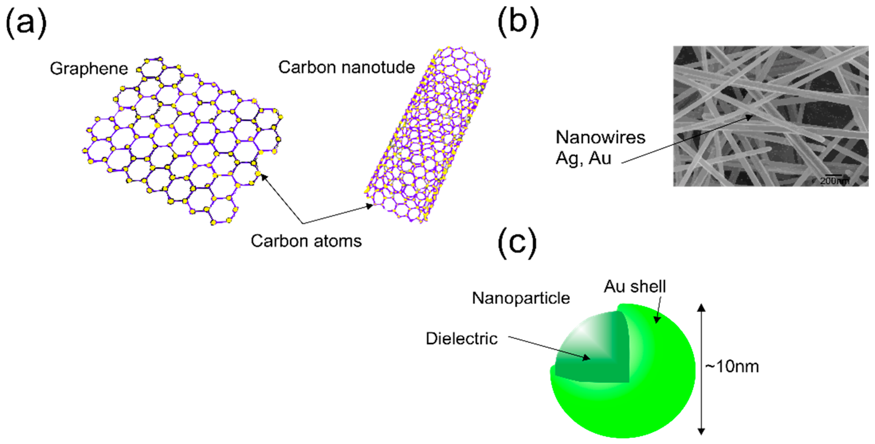
2.2. Nanomaterial-Based Sensors

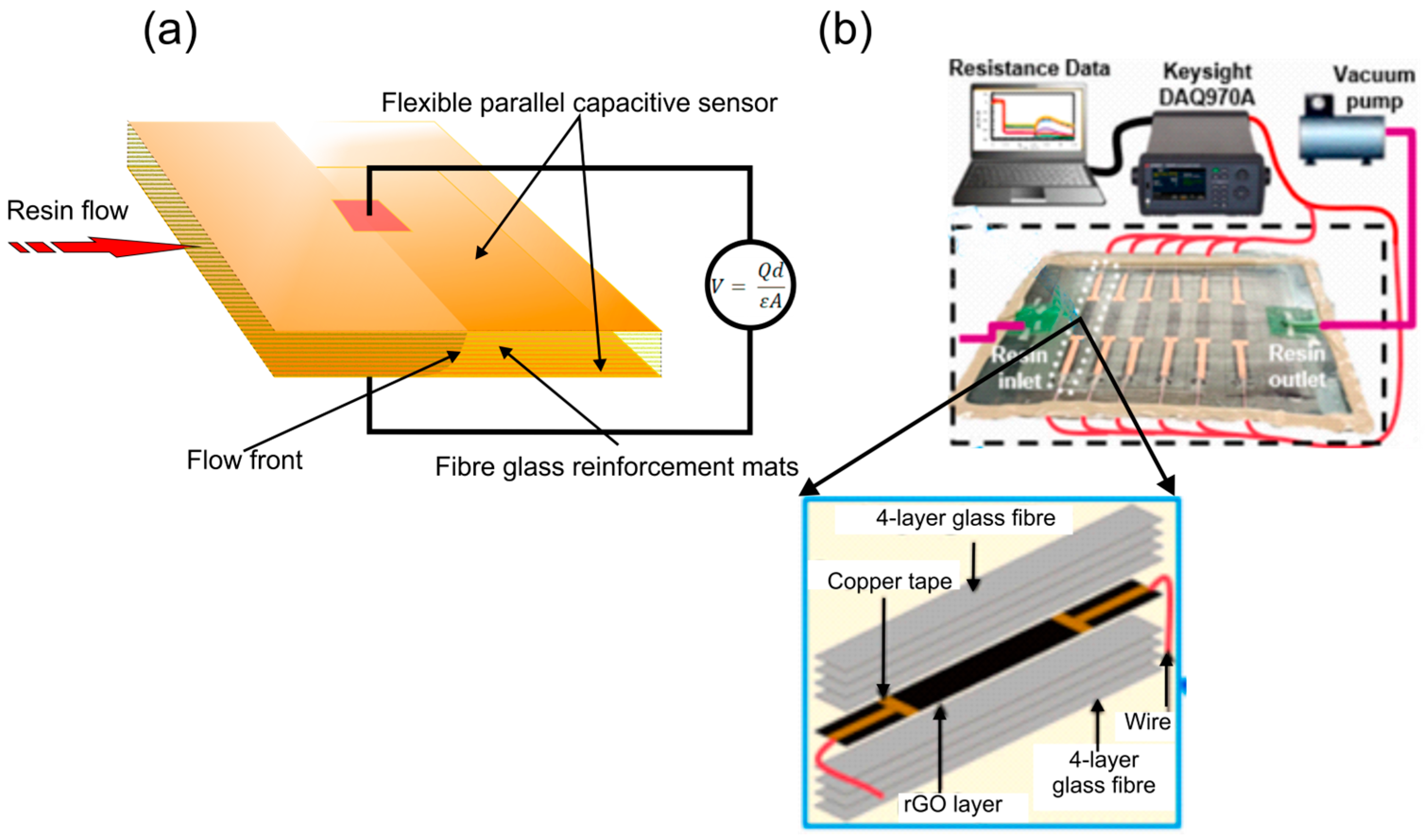
There are many variations of nanomaterials based upon the exploitation of the changes in their physical properties due to changes in the environmental conditions, such as temperature, stress/strain, and chemicals that generate changes in electrical properties, such as resistance, capacitance, or optical properties, or permittivity (refractive index) [91,92]. There are a large variety of nanomaterials but there are three main groups that are being developed, investigated, and used in different applications; these are carbon nanotubes (CNTs), metal nanoparticles (mNPs), nanowires, and Graphene (see Figure 6) [93]. CNTs, is one of the most widely used 1D nanomaterials and ha been previously utilised for the fabrication of various high-performance sensors and biosensors due to their unique mechanical, electrical, and magnetic properties [94,95]. Other types are carbon nanofibers (CNFs) that have been widely studied due to their unique chemical and physical properties and similar structure to fullerenes, and CNTs [96,97]. CNTs are hollow tube-shaped with a graphite layer parallel to the axis of the inner tube. The graphite layers of CNFs often form an angle with the axis of the inner tube, and the interior thereof may be hollow or solid. The diameters of CNTs are usually less than 100 nm, while the diameters of CNF are in the range of 10 to 500 nm and their length can reach 10 µm.

Graphene is another nanomaterial being used that consists of sheets of carbon atoms in a two-dimensional honeycomb lattice. It is the basic structural element of other carbon allotropes, including graphite. There are three main properties of interest for the applications that are being considered. One: The graphene sheet is a good electrical conductor that is approximately 10⁶ S/m at room temperature (300 K) [98]. The electrical conductivity varies due to other factors during fabrication like carrier density, impurities, and defects within the graphene. Two: The temperature dependence of graphene’s conductivity arises from scattering mechanisms that affect charge carrier mobility, such as phonon scattering and the thermal vibration of carbon–carbon bonds. Considering a single monolayer of graphene, the electrical conductivity σ can be approximated as $\sigma \left(T\right)\approx {\displaystyle \frac{ne{\mu }_0}{1+\alpha T}}$, where n is the carrier density; this refers to the number of charge carriers (electrons or holes) per unit area or volume in a material. The unique band structure graphene plays an important role in this parameter, where e is the charge of an electron, μ₀ is the mobility at a given temperature, α is the coefficient representing the rate of mobility reduction with temperature, and T is temperature in Kelvin [99]. Three: The thermal conductivity of graphene is ~5000 W/m/K, which makes the material a very good thermal conductor [100].

The electrical conductivity of graphene has a dependence upon graphene’s electronic properties that can be altered by stressed or strained the material, which in turn alters the charge carrier mobility, thus altering the conductivity. The stress/strain change localised electron density and, thus, affect the scattering processes, which alters the mobility of carriers. Typically, the strain-induced ripples or lattice deformations reduce mobility and lowers conductivity. The dependence of graphene’s conductivity σ on strain ε is given as $\sigma \left(\epsilon \right)={\sigma }_0\mathit{exp}\left(-\beta \epsilon \right)$, where σ₀ is conductivity of the material with no strain, β is the strain sensitivity coefficient of the graphene, and ε is strain [101]. The β (strain sensitivity coefficient) can vary depending on the magnitude of the strain and the specific strain conditions being applied to the material and the resultant deformation, such as the strain type (uniaxial, biaxial, or shear). Thus, the magnitude of the strain affects the electrical conductivity; usually, the strain is measured in microstrains (με). The sensitivity coefficient with respect to strain is given by a parameter called the gauge factor (GF), which relates the fractional change in resistance (ΔR/R) to the applied strain (ε) $GF={\displaystyle \raisebox{1ex}{$\Delta R$}\!\left/ \!\raisebox{-1ex}{$R$}\right.}/\epsilon$. The gauge factor and strain sensitivity coefficient with respect to conductivity vary with various kinds of graphene. Some examples are pristine monolayer graphene β from −0.2% to +0.4% as a percentage change along with a gauge factor of ~2, and Ag-doped graphene β from 20% as a percentage change along with a gauge factor of 177 [102,103,104,105].

Capacitive Sensors

Capacitive sensors are another classification of sensors used for monitoring in the manufacturing processes of fibre-reinforced polymeric structures. These sensors are used at various stages of production of the composites, as several physical parameters can affect changes in the capacitance, such as permittivity and thickness [106]. There are many examples of capacitive sensors being used at various stages of the manufacturing process, like resin flow, monitoring the resin flow into the mould (infusion), which is important in resin transfer moulding (RTM) and vacuum-assisted resin infusion (VARI). The sensing mechanism is based upon the change in the dielectric permittivity of the section of the moulding. This comes from the expression for capacitance $C={\displaystyle \raisebox{1ex}{${\epsilon }_r{\epsilon }_{0}A$}\!\left/ \!\raisebox{-1ex}{$d$}\right.}$, where c is the capacitance, ε_r is the relative permittivity (dielectric constant) of the material (mould), ε₀ is the permittivity of free space (8.85 × 10⁻¹² Fm⁻¹), A is the area of the electrode, and d is the separation of the electrodes (m) [107]. As the resin impregnates the reinforcement fibre in the mould, the relative permittivity (ε_r) and d change, which affects the capacitance and enables real-time monitoring [108,109]. Furthermore, during the curing process, the resin’s relative permittivity changes; thus, the curing process can be monitored in real time [110]. The chemistry will not be covered here in this review.

There are many different physical configurations for a capacitive sensor, such as the basic design shown in Figure 7, which is a flexible membrane situated into the mould itself [111] (see the schematic shown in Figure 7a) and a series of line electrodes from an experimental setup [112], as shown in Figure 7b.

Another parameter the capacitive class of sensor is used to measure is the fibre volume fraction measurement; this is the fibre-to-resin ratio that affects the permittivity (ε_r) by producing an effective dielectric/permittivity for the material from the fractional volume of the fibre to the resin. There are several strategies to evaluate this effective permittivity, such as the Maxwell Garnett and Bruggeman effective medium theories for the average permittivity of a dielectric for inhomogeneous materials [113,114,115]. Thus, the effective/average permittivity is ${\epsilon }_{eff}={\epsilon }_{Resin}·V_{resin}+{\epsilon }_{Fibres}·V_{Fibres}$, where ε_eff is the effective permittivity of composite and ε_Resin, ε_Fibres are the permittivity of the resin and fibres, respectively, and V_Resin, V_Fibre are the volume fraction of resin and fibres, respectively.

The capacitive sensors are used to monitor the curing process of the resin/epoxy used in conjunction with glass reinforcement mats [116,117]. There are three main stages of the curing of the resin in a mould for fibre-reinforced polymeric structures. After the impregnation of the glass mats by the resin, the first stage is the gelation. The resin begins to thicken, and this is the phase change from a liquid to solid; chemically, the molecules start the cross-linking process. The resin’s viscosity increases significantly at this stage. This also changes the effective permittivity and, thus, the capacitances of the mould environment [118,119]. The “cross-linking” is an exothermic reaction and heat is generated within the mould. This is the second stage, and the heat generation helps to accelerate the curing of the resin. Again, effective permittivity is a function of temperature; thus, the capacitances of the mould environment change [120]. In the third and final stage, the resin reaches its maximum cross-linking where it approaches its full hardness. The cured polymer network is stabilised; again, the completion of the reaction changes the effective permittivity of the mould environment [118,119]. The degree of polymerisation affects the permittivity, providing the potential for real-time data on curing progression [120].

There is another major classification of sensors used in the manufacturing of FRP structures, namely, ultrasonic sensor/sensing for inspection of the structures for dry patches and fault lines (cracks) [120]. This procedure usually occurs after the manufacturing process has been completed and the resin has been cured [121,122,123]; thus, they cannot be classified within the real-time monitoring.

3. Implementation of Sensors: Arrays and Multiplexing

This topic needs dedicated consideration, and there are several reasons for adopting this approach, particularly when evaluating critical attributes. These attributes are closely linked to the characteristics of the various sensor types previously discussed. The performance specification of any sensor array depends on a range of factors, as outlined below. The authors note that this topic has been extensively investigated by numerous researchers, resulting in a substantial body of literature covering the various aspects discussed herein. In this section, the authors outline the key characteristics to be considered and provide meaningful comparisons, supported by references for further reading.

(i)

The capability of multiplexing of sensors: This is important with regard to the spatial resolution of a measurement for a specific parameter. An example is the monitoring of the flow front of the resin within the mould, to ensure complete impregnation of glass fibre reinforcement mats to avoid dry spots that can act as induced cracks within the structure and may prove to be catastrophic for a structure [124,125]:

(ii)

The ease of interrogation of sensors/sensor array: This can be a limiting factor in using a specific sensing scheme and can relate to the response time of scheme to obtain a measurement. A quicker response may be desirable to react to a given set of measurements. Also, the interrogation scheme itself may have limitations on the number of sensors it can monitor in total in a reasonable or required time interval. Furthermore, the interrogation scheme itself can have a limit on the spatial resolution, such as SBS or OTDR, which ha a spatial limit on the order of ~0.5 m [126]. Also, interrogation can be complicated because of cross-sensitivity [127] between various parameters, like temperature and the presence of resin/epoxy (changing the permittivity), which leads to misinterpretation. Another overriding factor may be the cost of the interrogation scheme (financial restrictions; too expensive to implement).

(iii)

The survivability and reliability of the sensing array; These two attributes refer to practical solutions if there is damage to the sensing array and its abilities to perform the sensing activities to the desired specifications after damage has occurred [128]. Here, “practical solutions” refer to the following: firstly, reasonable costs in hardware as well as other aspects including installation and maintenance and also reliability/durability of the sensing to perform over the required time span. Secondly, to accidental damage of the sensing array, meaning to individual sensors or number of sensors within the array and its ability still to be used as a sensing array yielding meaningful measurements and data [129]. In order to guarantee steady and reliable sensing service, large-scale sensor networks require high “robustness”, which is the ability to maintain system functionality against external and internal interference. Extensive research on the reliability and survivability/robustness of sensing networks with unconventional array architecture, such as a fishnet approach, is given in Refs. [130,131].

(iv)

Interpretation of the response of the sensing array design: This topic has created different approaches from machine learning algorithms (pipes) to direct measurement with optimum sensors and location. This is very much dependent upon the environment in which the sensing array/network is operating and varying the number of parameters that affect the sensor’s performance and measurements [131,132,133,134].

(v)

The practical implementation (lay-up) of sensing schemes in a workplace: In practical implementation, the lay-up of a sensing scheme within a mould during the liquid composite moulding process requires careful planning to ensure effective integration without disrupting the flow of resin or the structural integrity of the final composite. Sensors—such as fibre optic or piezoelectric types—are typically positioned either on the surface of the mould or embedded within the reinforcement layers, depending on the monitoring objective. Their placement must accommodate resin flow paths, curing behaviour, and fibre architecture, while ensuring reliable data acquisition. Secure fixation and appropriate protection of the sensors are essential to prevent displacement or damage during infusion and curing stages. Due to the nature of the process, the sensor fibres have to remain in the structure. If the sensor fibres are significant in number (a network of fibres), it is vital to consider the adhesion of the resin with the sensor fibres. In general, the fibres used as reinforcement are processed with sizing to achieve good adhesion with fibre interface and the resin [135]. For the sensor fibres, such sizing may not be available, which may result in poor adhesion at the interface of sensor fibres and resin; these sites can act as induced cracks in the structure. The size of the sensor fibre can play a significant role in the practical implementation as its diameter is often considerably larger than that of the reinforcement fibres. This mismatch can lead to local disruptions in the fibre architecture, potentially affecting resin flow, wet-out, and even creating resin-rich zones or voids. Careful consideration must, therefore, be given to sensor selection and placement to minimise such disturbances and ensure reliable integration.

3.1. Comparison of Sensor Performance

Numerous competing techniques and technologies exist for monitoring the manufacturing processes of fibre-reinforced polymeric structures. Direct comparison of the various measurands associated with the performance of each interrogation method and sensor is not necessarily meaningful. Instead, a focus on overarching characteristics that are applicable across all sensing technologies is more constructive. Accordingly, the principal types of sensing approaches and the attributes of their respective sensors are examined individually. The following parameters are, therefore, considered within the general performance tables for each sensor type presented below:

Spatial resolution: This is the general performance of an individual sensor to detect the measurand. This parameter is included for spatial location to determine the resin flow front during infusion.

Accuracy: This is given as an overall error in the detected/monitored measurand value by the interrogation scheme, working in conjunction with the sensor and given as a percentage to make an easier comparison.

Sensitivity type parameter: The key environmental parameters considered across all three stages are critical in the fabrication of FRP composite structures: (i) during the lay-up stage, measurements of curvature, pressure, and strain [136]; (ii) during the infusion stage, measurements of the resin content index (which indicates the presence of resin and detects dry patches), temperature variations resulting from the temperature difference between the resin and the mould/glass reinforcement mats, and strain caused by the advancing flow front, which induces compression [137]; and (iii) during curing, the changes in material composition (due to the curing process) alongside temperature variations, as curing is an exothermic reaction, with strain increasing throughout the process [138].

Multiplexed sensor number: This is number of sensors used in the experiments. If the sensing scheme is distributed, the number given is the number of locations where measurements are taken in the investigation [139].

Response time: This is the time taken in obtaining datum from the sensing scheme.

Sensing range: This is the maximum distance that an individual sensor can detect a measurand.

In addition to the general performance tables, these are followed by a second table relating to general attributes that would be of interest to researchers considering using these techniques in the production of FRP composites structures. These are the following: (i) Implementation with specific possible issues mentioned, such as contacts, a complex design, or fragility. (ii) Survivability routes, referring to the alternative routes available if the sensing array is to measure and convey that information. (iii) Reliability issues, where there could be weaknesses with regard to robustness or incurred errors reducing performance. These are the general physical attributes of interest during the manufacturing process of the composite structure.

Table 1. General performance of capacitive sensors.

Sensors	Reference	Spatial Resolution (m)	Error %	Sensitivity Type Parameter					Multiplexed Sensor Number	Response Time	Sensing Range (m)
				Index	Temperature	Strain	Curvature	Other		(s)
Capacitive	[116]	~0.04	~2	✓	✓	✓	?	_	Distributed	~4	~1
Capacitive	[117]	~0.02	~7	✓	✓	✓	×	Pressure	Distributed	~1	_
Capacitive	[140]	~0.01	~2	✓	✓	✓	×		Quasi Distributed	~5	_
Capacitive + FBG	[141]	~0.1	~0.2	✓	✓	✓	×	Pressure	5 section and 1 Distributed	~16	Few
Capacitive +Graphene	[142]	~0.02	_	✓	✓	×	×		Distributed	~20	_
Capacitive	[143]	_	~3	✓	✓	✓	×	Pressure	Distributed	~1	Few
Capacitive	[144]	~0.01	~3	✓	✓	×	×		Distributed with 10 points	~4	Few

and

Table 2. General attributes of capacitive sensors.

Sensors	Reference	Implementation	Survivability Routes	Reliability Issues	Flow-Front	Curing	Defects
Capacitive	[115]	Plate intergation	1	Bending, Coupling	✓	✓	✓
Capacitive	[116]	Electrodes	1	Interpretation	✓	✓	✓
Capacitive	[140]	Electrodes	1	Intergated response	✓	✓	✓
Capacitive + FBG	[141]	Complicated arrangement	1	Cross -talk	×	✓	✓
Capacitive + Graphene	[142]	Complicated arrangement	1	Cross -talk, Interpretation	×	×	×
Capacitive	[143]	Mould design	1	Cross -talk, Interpretation	✓	✓	×
Capacitive	[144]	Plate intergation	1	Interpretation	✓	✓	✓

give the overall performance of the capacitive sensors. The general observation is that the capacitive sensors are distributed with measurements at different locations, with electrodes contacted at separate locations. This will give different temporal responses of the sensor and, thus, yield the issue of interpretation of the capacitor sensor’s response to the various parameters with the additional problem of cross-sensitivity. The majority of the capacitive sensors [116,117,139,140,141,142,143] are suitable for measuring three major parameters: index, strain, and temperature. The sensing range is low, which makes this sensing approach less favourable for large composite structures. The potential advantage of capacitive sensors is shown in Table 2; they all appear to have the ability to detect the three major problems in the manufacturing process: flow front, ensuring that the mats are completely wetted that curing can be completed, and detecting defects.

The main advantages of capacitive sensors and their interrogation schemes lie in the monitoring of the processes during FRP manufacturing. Real-time monitoring can be performed to detect the resin infusion and curing [115,116,140,141,142,143,144]; this is not a true tracking of the resin flow front through the mould itself but it can be used to realise full impregnation of the mats by the resin and offers a feedback signal for process adjustments. The issue with the monitoring of the infusion and curing is the misinterpretation of the readings due to cross-sensitivity with other environmental parameters, such as moisture, temperature fluctuations, or conductive contaminants [106]. Another issue is the sensing locations (electrodes). Altering the spatial location of the electrodes and positioning of the dielectric layers (glass reinforcement mats, fill-factor [113,114,115]) will yield a different response with the same mould. This spatial dependence of the capacitance will create complex calibration and manufacture procedures for the precise alignment of electrodes and dielectric layers to ensure accurate measurements. This situation is further complicated by load orientation on the glass reinforcement mats, which changes the fill-factor and, thus, the permittivity. In addition, this sensing technique has limited spatial resolution (see Table 1 references) and has only been applied to smaller FRP composite structures. Whilst the capacitive sensor approach may be complex, it offers the potential to detect damage or defects in their early stage (dry spots, voids, delamination) by changing the permittivity [115,116].

Table 3. General performance of optical fibre Bragg grating sensors.

Sensors	Reference	Spatial Resolution (m)	Error %	Sensitivity Type Parameter					Multiplexed Sensor Number	Response Time	Sensing Range
				Index	Temperature	Strain	Curvature	Other		(s)	(m)
FBG	[145]	~0.04	~3	✓	✓	✓	✓	_	24 FBG	~60	~5000
FBG +PZT	[146]	~0.07	~5	✓	✓	✓	×	_	Distributed + 9 FBG	~1	Few
FBG +PZT	[147]	~0.01	~2	✓	✓	✓	×	_	9 PZTs + 14 FBG	~1	Few
FBG+OFDR	[148]	~0.03	~10	×	✓	✓	×	_	Distributed	~1	~1
FBG	[149]	~003	~5	×	✓	✓	×	_	10 FBG	~1	~1
FBG+Fresnel	[150]	~0.05	~2	✓	✓	✓	×	Polarisation	10 Fresnel + 5 FBG	1	3
TFBG +Fresnel	[151]	~0.001	~10	✓	✓	✓	×	Polarisation	1TFBG + 1 Fresnel	~1	~0.5
EFPI sensor +FBG	[152]	~0.001	~5	✓	✓	✓	×	_	1 EFPI + 1 FBG	~10	~0.5

and

Table 4. General attributes of optical fibre Bragg grating sensors.

Sensors	Reference	Implementation	Survivability routes	Reliability Issues	Flow-Front	Curing	Defects
FBG	[145]	WDM	2	Losses, Coupling	✓	✓	✓
FBG +PZT	[146]	Complex. Wires layout	1	Cross-talk	✓	✓	×
FBG +PZT	[147]	Complex. Wires layout	1	Fragile connectors	✓	✓	×
FBG+OFDR	[148]	Simple	1	Cross -talk	✓	×	✓
FBG	[149]	Sensor in tows, Breakage	1	Cross -talk, Interpretation	✓	×	✓
FBG+Fresnel	[150]	Couplers	4	Cross -talk, Polarisation	✓	✓	×
TFBG +Fresnel	[151]	Couplers	4	Cross -talk, Polarisation	×	✓	×
EFPI sensor +FBG	[152]	Coupler, Fragile	1	Cross -talk, Polarisation	✓	✓	×

[145,146,147,148,149,150,151,152] give the overall performance of the optical FBG sensors with regard to the application of monitoring the production process of FRP composite structures. This sensing technology can be used in all three stages of production. Individual FBG sensors have good spatial resolution for measurement at that location [58,59] but these sensors are part of a sensing scheme that can yield good spatial resolution over a significant sensing range of up to 5 km with a measurand spatial resolution of 4 cm, which is promising for large FRP composite structures [145]. In general, these FBG sensing systems yield spatial resolutions of approximately 1 cm, which is a similar size and above that of defects of concern within a FRP composite structure, but the majority of the work performed to date is on smaller structures on the scale of few metres (see Table 3). Furthermore, the associated errors are small, yielding good accuracy for measurands being monitored along with a good survivability route [150,151]. However, cross-sensitivity remains a concern [59], as it can lead to misinterpretation and introduce additional errors. There is an additional issue of induced birefringence by compaction of the FBG caused by a vacuum; this is created by non-axial strain on the fibre leading to a complicated strain pattern over the volume of the optical fibre [61,62,63]. This degrades the spectral features of the FBG and potentially corrupts the sensing schemes performance and leads to misinterpretation of the measurand datum. These sensors may use different measurands, such as wavelength shift or the change in the optical strength of spectral features. FBGs can also be used as an effective mirror in the core of the optical fibre to be part of a cavity, such as extrinsic Fabry–Perot interferometer (EFPI) sensors at a selective wavelength (for wavelength multiplexing), using phase as a measurand [152], or a Fresnel optical sensor, which is a cavity based upon reflections at the interface of two differing materials with different refractive indexes working in conjunction with FBGs [150,151].

Optical Fiber Bragg Grating (FBG) and Tilted Fibre Bragg Grating (TFBG) sensors in FRP manufacturing do find applications in process monitoring due to their generally high sensitivity and accuracy of strain and temperature [58,59] and index [63]; thus giving precise strain and temperature measurements during resin infusion and curing, enabling real-time monitoring of composite processes. Compared to other sensing technologies, these sensors are easily multiplexed using series techniques such as wavelength division multiplexing or time division multiplexing [139] or using other multiplexing/interrogation techniques, like optical frequency domain reflectometry (OFDR) [148]. Therefore, a large number of these sensors can be used in a single optical fibre, allowing distributed strain monitoring along with the optical fibre being able to be embedded within the glass reinforcement mats without compromising the strength of the FRP composite structures.

There are limitations and weaknesses of using a sensing scheme based on FBG/TFBG sensors. The laying-up procedure for embedding the optical fibre can be complex, in addition to fragility issues: careful handling is required to avoid breakage of sensor fibres during the laying-up stage of production and issues of breakage during vacuum consolidation. Other considerations are also required in the laying-up process to ensure that there is no spectral feature corrupt from non-uniform strains [61,62,63] and that there are no loose fibre reinforcement mats. Resin shrinkage can cause uneven strain distribution; again, this would corrupt the spectral feature FBG and lead to additional errors. Furthermore, Table 3 shows that FBG sensing arrays have a limited sensing range for defects, such as dry patches or large-area defects (delamination), and, thus, would require dense sensor arrays. This would increase cost and, again, increase the complexity of the laying-up procedure. Finally, optical fibre interrogation systems are generally more expensive than other sensor interrogation schemes.

Table 5. General performance of piezo and piezo transducer sensors.

Sensors	Reference	Spatial Resolution (m)	Error %	Sensitivity Type Parameter					Multiplexed Sensor Number	Response Time	Sensing Range (m)
				Index	Temperature	Strain	Curvature	Other		(s)
PZT	[153]	~0.05	~5	×	×	✓	×	Sound, Lamb wave	9 PZT	~10	~0.5
PZT	[154]	~0.1	~8	✓	×	✓	×	Sound, Lamb wave	10 PZT	~10	~0.5
PZT+PVDF	[155]	~0.05	~5	✓	✓	✓	×	_	4 PZT	~1	~0.5
PZT	[156]	~0.12	~5	×	✓	✓	×	Pressure	5 PZT	~20	~0.6
PZT	[157]	~0.05	~10	✓	×	✓	×	Sound, Lamb wave	9PZT	~0.001	~0.6
PZT	[158]	~0.06	~7	✓	×	✓	×	Sound, Lamb wave	18 PZT	~0.001	~0.6
PZT	[159]	~0.001	~3	×	✓	✓	×	Lamb wave	1 PZT	~0.1	~3.0
PZT+ Carbon nanomaterial	[160]	~0.014	~5	✓	✓	✓	×	Resistance	36 Sensors	~5	~0.3

and

Table 6. General attributes of piezo and piezo transducer sensors.

Sensors	Reference	Implementation	Survivability Routes	Reliability Issues	Flow-Front	Curing	Defects
PZT	[153]	Contact wires	9	Contacts, Cross-talk	✓	✓	×
PZT	[154]	Contact wires, Complex wiring	10	Cross-talk	✓	✓	✓
PZT+PVDF	[155]	Complex layup procedure, Breakage	4	_	✓	✓	×
PZT	[156]	Complex layup procedure	5	Contacts, Interpretation	✓	×	✓
PZT	[157]	Complex layup procedure	5	Cross-talk	✓	✓	x
PZT	[158]	Wire breakages	9	Cross-talk	✓	✓	✓
PZT	[159]	Complex layup procedure	1	_	×	✓	✓
PZT carbon nanomaterials	[160]	Contacts fragile, Complex layup procedure	18	_	✓	✓	×

[153,154,155,156,157,158,159,160] give an overall performance of sensors based on piezoelectric materials and transducers (PZT). This sensing mechanism approach can be used in all three main stages of the production process. The general performance of these types of sensors yielded mixed results, with a 6 PZT sensing scheme yielding spatial resolution of equal to or greater than 5 cm, which can restrict the systems from detecting defects unless the sensor density is increased. Increasing the sensor density can lead to other issues, such as making the laying-up procedure more complex and becoming more susceptible to human error. A significant number of these PZT sensing systems work in conjunction with the Lamb wave phenomena [86,87], which yielded reasonable results over small sensing ranges of three metres and less (see Table 5). There are several potential issues with using Lamb waves as part of the sensing strategy. These waves can have significant attenuation when passing through composite sandwich structures, thus reducing detection sensitivity. They are further complicated by the material/composite heterogeneity, such as FRP composites’ anisotropic properties and layered structures, leading to multiple Lamb modes that can lead to potential misinterpretation and, thus, additional errors [86,87]. Although arrays of up to 36 PZT sensors have been employed by researchers [160], this significantly increases the complexity of the lay-up process. While PZT-based sensing schemes provide a responsive system, they require careful calibration and interpretation of the resulting data.

In general, there are some potential advantages of using PZT sensors in the monitoring of FRP manufacturing processes, such as real-time monitoring of the resin flow front, curing progress, and defect formation during manufacturing. The references in Table 5 demonstrate the sensitivity of PZT sensors to curing parameters by using the Lamb wave. Furthermore, the PZT sensing scheme has been utilised as a multifunctional approach for monitoring resin infusion (flow front), degree of cure, and structural defects [158,159,160]. Also, this type of sensing scheme can be used in conjunction with other sensing approaches, like, FBG sensors for strain measurement, for enhanced accuracy in monitoring the curing process, and for damage detection [29]. There are issues with this sensing approach relating cross-sensitivity with temperature and other parameters of interest (see Table 6 references). In general, the use of PZT yields an overall response at the specific location of the PZT and with limited spatial resolution, and the data needs to be analysed rigorously to ensure that the correct interpretation is obtained.

Table 7. General performance of nanomaterial sensors.

Sensors Nanomaterials	Reference	Spatial Resolution (m)	Error %	Sensitivity Type Parameter					Multiplexed Sensor Number	Response Time	Sensing Range (m)
				Index	Temperature	Strain	Curvature	Other		(s)
Nano carbon-reinforced sensors	[161]	~0.01	~3	×	×	✓	×	Pressure /Resistance	9 sensors	~1	~0.5
CNT	[162]	~0.015	~1	✓	✓	×	×	Pressure /Resistance	5 sensors	~1	~0.1
Graphene	[163]	~0.02	~2	✓	✓	×	×	Resistance	20 sensor	~1	~0.4
MWCNT	[164]	~0.01	~3	✓	✓	×	×	Resistance	7 sensors	~1	~0.2
Graphene	[165]	~0.01	~1	✓	✓	×	×	Resistance	8 sensors	~2	~0.2
Fibre-reinforced polymer	[166]	~0.04	15	✓	✓	×	×	Guided ultrasonic wave	8 sensors	~0.00001	~0.5
Carbon fibres	[167]	~0.02	~5	✓	×	×	×	Resistance	8 sensors	~1	~0.2
Carbon fibres/Teflon	[168]	~0.05		✓	×	×	×	Resistance	16 sensors	~1	~0.2
CNT	[169]	~0.03	~3	✓	✓	×	×	Resistance	7 sensors	~1	~0.3

and

Table 8. General attributes of nanomaterial sensors.

Sensors Nanomaterials	Reference	Implementation	Survivability Routes	Reliability Issues	Flow-Front	Curing	Defects
Nano carbon-reinforced sensors	[161]	Complex layup procedure, Fragile	4	Contacts, Cross-talk	✓	×	×
CNT	[162]	Contact wires	3	Cross-talk	✓	✓	×
Graphene	[163]	Complex layup procedure	10	Cross-talk	×	✓	✓
MWCNT	[164]	Complex layup procedure	4	Contacts, Cross-talk	✓	✓	✓
Graphene	[165]	Complex layup procedure	4	Cross-talk	✓	✓	✓
Fibre-reinforced polymer	[166]	Wire breakages	4	Cross-talk	✓	✓	✓
Carbon fibres	[167]	Wires complex layup procedure	3	_	✓	×	✓
Carbon fibres/Teflon	[168]	Contacts, complex layup procedure	8	Cross-talk	✓	✓	×
CNT	[169]	Contacts, complex layup procedure	4	_	✓	✓	×

[161,162,163,164,165,166,167,168,169] show the use of nanomaterial sensors and sensing schemes in the manufacturing processes of FRP structures for monitoring resin infusion, resin curing, and defects. This is a recent application for nanomaterials, such as graphene or carbon nanotubes (CNTs) and multiwall carbon nanotubes (MWCNTs). The first observation on the reported research activities is that all investigations are performed on small dimension moulds of the order of ~0.5 m²; thus, there is a question of scalability for larger FRP structures to use this sensing approach. The spatial resolution yielded by the use of nanomaterials is approximately 1 cm, which is suitable for defect detection and resin flow front monitoring, with an estimated sensing range of around 0.2 m. However, this necessitates a high density of sensors, electrodes, and connecting wires, which increases the complexity of the lay-up process [162,165] and raises the likelihood of wire breakage at the contact points with the CNTs. Furthermore, there are additional processes needed for the nanomaterial sensors, e.g., the consolidation of CNTs or graphene with resin along with the glass reinforcement mats [161,162,163,164,165,166,167,168,169]. The major advantage of this type of sensing system is the survivability of the monitoring system. Cross-sensitivity has an issue with temperature but still has a reasonably favourable accuracy compared to other sensing systems (see Table 8).

The main advantages of nanomaterial sensors in FRP manufacturing yields enhanced sensitivity along with real-time monitoring of resin flow, curing kinetics, or/and defect detection [170]. Secondly, the integration versatility of conductive nanomaterials, such as graphene and carbon nanotubes (CNTs), enhances the electrical connectivity in non-conductive fibres without compromising the mechanical robustness of the composite structure [171]. There are, at present, several issues that need to be addressed with nanomaterial sensors, like the complex manufacturing process [161,162,163,164,165,166,167,168,169,170,171]. An example of increased complexity is the production process, such as the addition of physical vapor deposition (PVD) or other coating techniques that require additional equipment and expertise that increase production costs [170]. Furthermore, regarding scalability, the examples presented in the literature to date have primarily involved small FRP structures (see Table 7). Additionally, the use of materials such as gold and graphene contributes to increased costs [171].

There has been significant research interest in recent years in the use of distributed sensing techniques for monitoring the manufacturing processes of FRP composite structures (see

Table 9. General performance of optical fibre distributed sensors.

Distributed Sensors	Reference	Spatial Resolution (m)	Error %	Sensitivity Type Parameter					Multiplexed Sensor Number	Response Time	Sensing Range (m)
				Index	Temperature	Strain	Curvature	Other		(s)
Rayleigh scattering +OFDR	[172]	~0.005	~8	✓	✓	✓	×	Polarisation	4	~1	~1
Rayleigh scattering	[173]	~0.005	~6	×	✓	✓	×	Polarisation	1	~0.1	~4
Rayleigh scattering +OFDR	[174]	~0.01	~10	×	✓	✓	✓	Polarisation	1	~0.1	~0.3
Rayleigh scattering + OFDR	[175]	~0.01	~3	✓	✓	×	×	Polarisation	5	~0.1	~0.5
BOTDR +WDM	[176]	~0.05	~5	×	✓	×	×	Polarisation	1	~1	~50,000
BOTDR + Raman	[177]	~0.1	~5	✓	✓	×	×	_	1	~1	~100,000
BOTDA +Au coating	[178]	~0.01	~5	✓	✓	×	×	Polarisation	1	~1	80
Raman + OTDR	[179]	~0.01	~5	×	✓	×	×	_	1	~1	~25,000
Raman + Differential pulsewidth pair detection	[180]	~0.004	~3	✓	✓	×	×	_	1	~1	6000

and

Table 10. General attributes of optical fibre distributed sensors.

Distributed Sensors	Reference	Implementation	Survivability Routes	Reliability Issues	Flow-Front	Curing	Defects
Rayleigh scattering +OFDR	[172]	Expensive equipment	2	Cross-talk, Polarisation	×	✓	×
Rayleigh scattering	[173]	Expensive equipment	1	Cross-talk, Polarisation	×	✓	×
Rayleigh scattering +OFDR	[174]	Complex layup procedure	1	Cross-talk, Polarisation, Temperature	×	✓	×
Rayleigh scattering + OFDR	[175]	Expensive equipment	2	Contacts, Cross-talk	×	✓	×
BOTDR +WDM	[176]	Complex layup procedure	1	Cross-talk	×	✓	×
BOTDR + Raman	[177]	Complex layup procedure	1	_	✓	✓	×
BOTDA +Au coating	[178]	Complex layup procedure, Expensive equipment	1	_	✓	✓	×
Raman + OTDR	[179]	Complex layup procedure	1	Cross-talk	✓	✓	×
Raman + Differential pulsewidth pair detection	[180]	Complex equiment	1	_	×	✓	×

) [172,173,174,175,176,177,178,179,180]. Firstly, these techniques demonstrate considerable potential for application in larger composite structures [8,9,10], with sensing ranges exceeding 5 km [176,177,179,180]. However, their main limitation lies in the relatively low spatial resolution—typically greater than 1 m (see Table 9), which means that small defects, such as microvoids, may go undetected. This poor spatial resolution also means that this sensing approach is not appliable for monitoring the flow front of the resin. Furthermore, the accuracies of these systems are generally less than other sensing approaches, like FBG sensors (see Table 3). In addition, there is an issue with polarisation noise that can affect the overall performances of these distributed sensing approaches.

Raman distributed optical fibre sensing (RDOF) schemes offer long sensing ranges, capable of monitoring large structures such as wind turbine blades and aerospace components over distances extending up to several kilometres (see Table 9). Furthermore, RDOF is primarily sensitive to temperature, which eliminates cross-talk from other environmental parameters, making it an ideal candidate for monitoring the curing process. However, its application is limited in measuring or detecting the initial resin flow front.

There are other distributed sensing approaches based upon Brillouin scattering, Brillouin optical time domain analysis (BOTDA), and Brillouin optical time domain reflectometry (BOTDR) that, again, have long sensing ranges that have both temperature and strain sensitivity; however, the strain sensitivity varies between 20 με and 60 με [126,127], which may be useful to detect defects. The strain generated by the resin flow front is approximately ±30 με from Ref [181]; this implies that the strain sensitivity is not enough in itself to monitor the flow front of the resin directly. The sensing range for BOTDA and BOTDR ranges from ~1 km to ~150 km [127] with spatial resolutions of ≤1 cm for both Brillouin approaches. There is potential for misinterpretation of data from the sensing scheme due to the fact that the modelling of mould status (the resin curing degree) correlates to the Brillouin frequency shifts [175] and the interrogation equipment is expensive.

Another sensing technology being investigated is Rayleigh scattering and optical frequency domain reflectometry (ROFDR) [172,173,174,175]. This technique monitors both strain and temperature with a spatial resolution of ≤1 cm, and the cost compared to other distributed sensing schemes is less expense [126]. This issue here is that the maximum sensing range, to date, is a few metres (see Table 9), so it is suitable for smaller FRP composite structures. There are other issues with the ROFDR, such as the ambiguity to which environmental parameter is causing the measurand to change [126,172,173,174,175]. Also, there is a potential issue arising from polarisation induced by birefringence [182].

There is another class of sensors that are like nanomaterial sensors but are considered separately; these are called piezoresistive sensors. They use similar materials, such as CNTs, MWCNTs, and graphene/graphene oxide [183,184,185,186,187,188,189]. These types of sensors are being investigated due to their relative ease of preparation. Also, these piezoresistive sensors have high sensitivity gain factors ranging from ~15 to ~100 [183,184,185,186,187,188,189]. The gauge factor and the physical properties are mentioned in a previous section “nanomaterial sensors”. Here, $GF={\displaystyle \raisebox{1ex}{$\Delta R$}\!\left/ \!\raisebox{-1ex}{$R$}\right.}/\epsilon$; again, ΔR/R is the net fractional change in resistance of the mould but measured at an electrode and ε is the strain subjected to the FRP composite generated by changing environmental parameters (temperature, curing, etc). Thus, the resistivity (material intrinsic structure) of the material becomes the dominant factor in creating GFs.

Typically, the fibres that are part of the reinforcement mats that are used in FRP structures are either dipped in a solution containing the reactive material (i.e., graphene) or it is sprayed on. The alternative method used is that the reactive material is mixed with the resin [183,184,185,186,187,188,189]. The principle of this type of sensor is that fibres of the resin create conductive architecture throughout the FRP structure and the net electrical conductance of the FRP structure changes during the fabrication process due to the presence of the resin (additional material), stress (from curing of the resin), and/or temperature changes due to the exothermic reaction of the resin. All of these processes can cause additional strain through the FRP composite. There are three parts that contribute to the overall conductive/resistance: (i) the intrinsic resistance, which is the inherent resistance that is dependent upon electronic structure and properties; (ii) the contact resistance, which is the effective barrier between interfaces of two materials due to surface imperfects/defects; (iii) the tunnelling resistance, which is associated with the ability of the electrons to quantum tunnel or thermally assist hopping of a junction potential [165]. The majority of the reported work is using these as an integrated sensing system to obtain an overall response; thus, the interpretation of the results can be challenging for more complex mould geometries.

Table 11. General performance of piezoresistive sensors.

Sensors Piezoresistive	Reference	Spatial Resolution (m)	Error %	Sensitivity Type Parameter					Multiplexed Sensor Number	Response Time	Sensing Range (m)
				Index	Temperature	Strain	Curvature	Other		(s)
Graphene	[183]	~0.04	~6	✓	✓	✓	✓	Resistance	6 sensors	~5	Semi-intergated response
CNT	[184]	~0.04	~8	✓	✓	✓	✓	Resistance	5 sensors	~2	Semi-intergated response
Reduce Graphene oxide	[185]	_	~4	✓	×	✓	✓	Resistance	1 sensor	~1	Intergated response
CNT	[186]	~0.03	~5	✓	✓	✓	×	Resistance	1 sensors	~1	Intergated response
MWCNT	[187]	~0.02	~5	✓	✓	✓	×	Resistance	1 sensors	~1	Semi-intergated response
Graphene	[188]	~0.03	~3	✓	✓	✓	✓	Resistance	3 sensors	~2	Semi-intergated response
Reduce Graphene oxide	[189]	_	~1	✓	✓	✓	✓	Resistance	3 sensors	~1	Semi-intergated response

and

Table 12. General attributes of piezoresistive sensors.

Sensors Piezoresistive	Reference	Implementation	Survivability Routes	Reliability Issues	Flow-Front	Curing	Defects
Graphene	[183]	Dip/Electrodes	Robust/ whole mould	Response change	✓	✓	×
CNT	[184]	Dip/Electrodes	Robust/ whole mould	Response change	✓	✓	✓
Reduce Graphene oxide	[185]	Dip/Electrodes	Robust/ whole mould	Response change	✓	✓	×
CNT	[186]	Dip/Electrodes	Robust/ whole mould	Response change	✓	✓	×
MWCNT	[187]	Dip/Electrodes	Robust/ whole mould	Response change	✓	✓	×
Graphene	[188]	Dip/Electrodes	Robust/ whole mould	Response change	✓	✓	×
Reduce Graphene oxide	[189]	Dip/Electrodes	Robust/ whole mould	Response change	✓	✓	✓

show some overall characteristics of the piezoresistive sensors used in monitoring FRP composite manufacturing processes.

Refs. [183,184,185,186,187,188,189] show that this sensing approach has potential, but there are caveats with this technique. All the piezoresistive sensing schemes yield either an integrated response from the mould, that is, a net variation with resistance as a function of time or a response or semi-integrated response relating to the number of contacts/electrodes used to monitor the mould process. Thus, the sensing system response needs to be calibrated to the specific mould so that there is no misinterpretation of the measurements of the sensing scheme. For simple geometries of the mould, like a straight stripe section, the resin flow front is flat front across the mould, but for more complex geometries, like moulds with curves, narrowings, etc., the interpretation is more challenging and benchmarks are required for each new mould, which would be time-consuming. Furthermore, there is a question to ask with this integrated approach: “Are the responses unique for different environmental conditions and mould physical status, the impregnation, curing, etc., or do the responses have some degree of degeneracy?” The alternative approach is to populate the mould with contacts to increase the density of measurements over more locations [183,187]. Increasing the number of contacts/electrodes for measurements would increase the complexity of the mould itself.

There are alternatives to the above sensing technologies.

Table 13. General performance of alternative sensors.

Sensors	Reference	Spatial Resolution (m)	Error %	Sensitivity Type Parameter					Multiplexed Sensor Number	Response Time (s)	Sensing Range (m)
				Index	Temperature	Strain	Curvature	Other
Ultrasonics	[190]	~0.001	~5	×	×	×	×	_	1	~1	~0.05
optical fibre losses	[191]	~0.1	~2	✓	x	✓	×	Pressure	5	~7	~1
infrared-thermal imaging	[192]	~0.001	~1	×	✓	×	×	_	1	~1	~10
Wireless sensor	[193]	~0.01	~2	✓	✓	×	×	Resistance	2	~1	~0.02
Ultrasonics	[194]	~0.001	~2	✓	×	✓	×	_	8	~1	~0.05
RFID	[195]	~0.01	~10	✓	✓	×	×	_	1	~5	~1
RFID	[196]	~0.02	~5	✓	x	✓	×		7	~10	~2
Thermocouples	[197]	~0.05	~3	✓	✓	×	×	Resistance	7	~1	~0.5
Long period gratings	[198]	~0.001	~5	✓	✓	✓	✓	Pressure	1	~1	~0.02
Long period gratings	[199]	~0.002	~5	✓	✓	✓	✓	_	1	~1	~0.02

and

Table 14. General attributes of alternative sensors.

Sensors	Reference	Implementation	Survivability Routes	Reliability Issues	Flow-Front	Curing	Defects
Ultrasonics	[190]	manual	1	large errors,	×	×	✓
optical fibre losses	[191]	layup breakages	3	cross-talk	×	✓	×
infrared-thermal imaging	[192]	complex equipment	1	_	✓	✓	✓
Wireless sensor	[193]	complex sensor	1	contacts, cross-talk	×	✓	×
Ultrasonics	[194]	complex layup	4	cross-talk	✓	✓	×
RFID	[195]	Fragile	1	_	×	✓	✓
RFID	[196]	complex layup	7	_	×	✓	×
Thermocouples	[197]	contacts, complex layup	7	_	✓	✓	×
Long period gratings	[198]	complex interrogation scheme	1	cross-talk,	✓	✓	×
Long period gratings	[199]	complex interrogation scheme	1	cross-talk,	✓	✓	×

show the other approaches that researchers are investigating [190,191,192,193,194,195,196,197,198,199]. This set of sensing approaches is briefly inspected here because there is a limited amount of material in the literature on these techniques. Ultrasonics is a conventional technology widely employed after the production of the FRP composite structure. This can be time-consuming for the system to maintain quality assurance and control and to initiate repairs; thus, it is not ideal for real-time monitoring and there is a potential waste of materials and production time [190,194]. The second group are the wireless sensors and radio-frequency identification (RFID) tags that are used to monitor the resin curing process by resistance changes; these can be used for temperature or strain and they yield real-time data. There are weakness with the RFID tags: they only measure at that location and have limited accuracy in measuring strain of ≤60 με [200]. Long-period grating sensors [198,199] have high sensitivities to all environmental parameters, but this makes cross-sensitivity a major issue (leading to misinterpretation) with these sensors. Furthermore, these LPG sensors have a complicated spectral response to all the measurands during manufacturing and compaction, leading to birefringence and corruption of the spectral features of the LPG sensors [63,64,201]. Whilst LPG sensors have issues, there is potential application for monitoring the resin flow front [198]. Infrared imaging [192] and thermocouples [198] have been investigated; firstly, the infrared imaging will yield flow and curing information but the spatial resolution depends upon the distance from the mould and depth into the mould to identify issues or monitoring resin flow front position [192], and the apparatus is used on a simple plane mould. The geometry of the mould can be a potential issue when using this technique. The thermocouples yield a reasonable small error of 3%, but the laying-up arrangement and procedure are complicated and increase with the number of thermocouples.

Data Management, Processing, and Interpretation

The above descriptions and comparisons of the challenges and issues arising from data acquisition using a sensor/sensor array is a non-trivial task, which makes it increasingly more difficult to make the correct interpretation of that real-time data. Researchers are now starting to use and develop pattern recognition algorithms in conjunction with an artificial neural network (machine learning algorithm) which is commonly known as artificial intelligence (AI); machine learning (ML), which inspects data and looks for patterns associated with given conditions [202,203,204,205,206]; along with the creation of “digital twins” [207,208]. These topics are worthy of discussion in their own right but a full description of these numerical methodologies and techniques is beyond the scope of this review.

A commonly used method is principal component analysis (PCA), which is an unsupervised machine learning algorithm that reduces the parameter space and looks for grouping in data [206]. Others are based upon signal/image processing techniques that involve convolution and self/cross correlation functions [209]. Other machine learning pipes (MLPs) are being used, like artificial neural networks (ANNs), which are a series of interconnected nodes that process and transmit information [206]. Another approach that can be proposed is the Uniform Manifold Approximation and Projection (UMAP) [210]; this is a dimensionality reducing algorithm. Effectively, UMAP takes many variable datasets, inspects those data for structures, and connects them, then creates a 2D or 3D representation of the data where the distances between data points represent local relationships as closely as possible [211]. An additional tool is Density-Based Spatial Clustering of Applications with Noise (DBSCAN). This is finding potential use in interoperating data from ultrasonic sensing arrays for detecting defects in carbon-fibre-reinforced plastics [212]. DBSCAN is a popular clustering algorithm used in machine learning to group data points that are close together (similar structure or dependency), while also identifying points that are far away from any group as outliers or noise.

Whilst these AI/ML approaches are gaining the attention of researchers, there are several issues that need to be considered when applying these techniques. Firstly, in the learning data for the AI/ML models, the data needs to be constructed in the appropriate format (independent and dependent variables) for the input or monitoring data, and the output data (resulting outcome) must be labelled to ensure that the data is unbiased, for example, there are no selection effects in the data or outputs. Secondly, the amount of data can be substantial for more complex composite structures, which can be time-consuming and expensive [205]. Therefore, it is important to ensure that there is no degenerate behaviour from the input data to the output data, which can lead to false outcomes. Hence, “the more data the better” and a greater number of independent parameters and associated datasets reduces the misinterpretation/error. There are other concerns associated with AI/ML models, like interpretability, uncertainty quantification (reliability/measurable errors in results), and explainability, e.g., why has the outcome happened, which is needed for a real-time monitoring system so that actions can be taken to counteract the bad outcome [205]. Furthermore, from the perspective of sensing schemes, it is important to ensure that there is a good signal/noise ratio, and independence of each sensor being used, along with a sensor density that is sufficient to ensure resolution in prediction (low uncertainty). In addition, it is important to ensure that the sensor location does not create bias in the input data when using these AI/LM models.

Another technique being used is “digital twins”, which are models/simulations run in real time using data from the sensors. The commonly used models are based upon finite element analysis (FEA) or finite element method (FEM) software [207,208,213]. These simulations use real-time data to (quantitatively) predict outcomes from the measurements given from the sensors. Both FEA and FEM simulations can produce “false” solutions; these appear to be correct within the software’s output but do not accurately represent the real-world behaviour of the analysed object from the sensor array dataset [214]. To have confidence in the FEA/FEM simulations, “benchmark” calibrations need to be performed. The creation of the model/simulation using the sensor dataset produces a result that is already known. Similarly to the AI/ML models, the higher the sensor density of the benchmark calibration, the less error of the known result will be generated. The development of these simulations can be time-consuming and expensive for large FRP composite structures and would need to be performed on each new structure. The authors would like to reiterate that this is a very brief descriptive overview of a large topic, and quantitative descriptions are beyond the scope of this review.

4. Discussion

The integration of sensing technologies into fibre-reinforced polymer (FRP) composite manufacturing presents a range of technical challenges, particularly due to the diversity and complexity of the processes involved. Techniques such as liquid composite moulding (LCM), prepreg lay-up, and resin transfer moulding (RTM) differ significantly in terms of flow dynamics, thermal profiles, and material handling, with each introducing distinct constraints for sensor implementation [215,216].

A central challenge arises from the physical disparity between sensor dimensions and the reinforcement fibres used in FRP systems. Carbon fibres, commonly employed in high-performance composites, typically have diameters of around 7 µm, while glass fibres may range from 10 µm to 20 µm depending on the grade and application [135,217]. In contrast, commonly used optical fibres for sensing—such as those based on fibre Bragg grating (FBG) technology—have cladding diameters of approximately 125 µm. This significant difference in scale can lead to localised disturbances in the fibre architecture, potentially altering resin flow, hindering impregnation, and resulting in defects, such as resin-rich zones or voids [60,218,219].

In LCM processes, the placement of sensors must be carefully planned to avoid obstructing resin pathways while still capturing meaningful data on flow front progression, temperature, or strain development. Improper placement or poor bonding between the sensor and the host material can compromise not only the quality of the measurement but also the integrity of the composite structure [9]. Similarly, in prepreg systems, embedding sensors without affecting layer compaction or resin distribution during curing is particularly challenging, as it can lead to delamination or stress concentrations [219,220].

Environmental factors also play a critical role in sensor performance during manufacturing. Elevated temperatures, pressure variations, and exposure to chemically reactive resins can degrade sensor materials or lead to signal attenuation over time [221]. Moreover, maintaining sensor calibration and data fidelity throughout the process and into service life adds another layer of complexity, particularly in embedded configurations where post-manufacture access is limited [22,151]. The above information from the various references [115,116,139,140,141,142,143,144,145,146,147,148,149,150,151,152,153,154,155,156,157,158,159,160,161,162,163,164,165,166,167,168,169,170,171,172,173,174,175,176,177,178,179,180,181,182,183,184,185,186,187,188,189,190,191,192,193,194,195,196,197,198,199] shows that different approaches are needed for the different production process; thus, it seems logical to consider the three stages individually along with a general sensing approach that can be possibly adopted. The first process is the monitoring of FRP composites for defects; this is probably the most challenging of the three issues during manufacturing. These include voids, dry patches, insufficient curing, and wrinkles or waviness. This relates to sensing range and the sensitivity of the sensing system being employed and needs to be considered from the laying-up of the glass reinforcement mats and to the final inspection. Whilst some of these techniques are showing potential, none have yet to demonstrate the detection of voids/dry patches of the size of 1 cm without a very high sensor density. The sensor densities required would be expensive and unrealistic for large FRP composites structures like aeroplane wings or fuselage and maritime wind turbine blades.

Firstly, for the laying-up of the glass reinforcement mats (GRMs), and the detection of wrinkles or waviness of the mats themselves, there are several potential sensing schemes; all of them are based upon optical fibres that can be woven into and laid between the mats. Placing sensor/optical fibres between the tows of GRMs and the additional GMRSs that are laid down on top will produce a small compaction force of the optical fibre and will be increased by the creation of a vacuum. The compaction of the optic fibre can be used to monitor the laying-up process; discrete sensors like the FBG and LPG are both sensitive to compaction force. The LPG has greater sensitivity to small transversal loads compared to the FBG, typically with limits of detection of ~15 kPa and ~0.1 MPa along with sensitivities of 4.6 × 10⁻¹ nm/kPa and 1.6 × 10⁻⁴ nm/kPa, respectively, before the onset of birefringence [198,222,223,224] for uniform loads. The presence of wrinkles or waviness of the mats will change the spectral response both in the linear wavelength response and the birefringence response regime. Furthermore, distributed optical sensors (based upon Brillouin and Rayleigh scattering) have a polarisation dependence [65,66,67,68,69,70]; thus, they are sensitive to birefringence but have a strain limit of detection (LOD) of ~10 με and ~0.1 m spatial resolution. There is potential for the distributed optical sensor to detect wrinkles or waviness if the spatial resolution can be improved.

Secondly, a process to consider is the resin infusion process. There are three candidates: FBG sensors, nanomaterial sensors, and piezo sensors. The main advantage of FBG sensors is their high sensitivity to strain changes, multiplexing capability, EMI immunity, and their ability to be used over hundreds of metres [145], yielding a direct measurement of the resin flow front [182]. However, there is the issue of cross-sensitivity with temperature [59] that needs to be considered. Recent research has shown that an FBG can directly monitor the force generated by the resin flow front, which generates a ~10 pm wavelength [225] which is approximately ~8 με. This is a small strain, but both nanomaterial sensors and capacitive sensors with LODs of 10⁻⁴ με and 10⁻⁵ με and sensitivities of ~0.1 V/με and ~5 V/με, respectively, can detect at this level of strain. The FBG spatial sensing location is effective as the sensor, and a ~10 cm radius of detection yields a sensor density of 25 sensors/m² to detect a 1 cm dry patch [225]. This would be a large number of sensors for large FRP composite structures and it would be costly to implement such a sensing scheme. The nanomaterial and piezo sensing schemes detect the total response of the mould and spatial resolution given by the number of the electrodes/contactors to measure the resistance or capacitance and detection ability of the whole structure. Thus, the sensor scheme can be associated with the mould and not the manufacturing of a single structure; this is a major advantage.

The nanomaterial sensors have great potential, as indicted from the references [161,162,163,164,165,166,167,168,169], with good temperature and index (permittivity) sensitivity for monitoring resin flow front, but the response measured is to the general condition or to the local condition and needs to be interpretated. Furthermore, the nanomaterial sensors may have a scalability issue; this approach has only been used on small structures of less than 1 m² and simple mould geometries (strips). Capacitive sensors have been shown to monitor the resin flow front and have high sensitivity to all parameters (index, strain, temperature) [115,116,141,142,144], but, again, cross-talk sensitivity is an issue. Furthermore, capacitive sensors have the same interpretation issue as nanomaterial sensors [113,115,164]. Overall, these three sensor types have advantages and disadvantages, with the nanomaterial sensor perhaps being the preferred choice. Even though nanomaterial sensors are a new sensing approach for this application, they have shown great potential, but the issue of mapping the sensor array’s response to real-time resin flow front location needs to be addressed for each new mould.

In the third process, the monitoring of the curing of the resin, there are three sensing types that appear to have a distinct advantage. The first of these are distributed sensors [172,173,174,175,176,177,178,179,180], which monitor the exothermic reaction and the strain (compaction of the resin) during gelatinisation to solidification. The distributed sensor will yield a general response of a mould, but spatial resolution can be a problem for optical lines over a hundred metres. The second and third sensor types are capacitive and piezoresistive sensors, because their responses are dependent upon permittivity/strain; again, spatial resolution can be an issue as increasing electrode numbers increases the complexity of the laying-up procedure [116,139]. Most of these researchers’ investigations have been performed on small areas of ~1 m² or less; therefore, there is a question of scalability. Quantifying this sensing attribute is challenging, and the curing of resin can relate to changes in various parameters: refractive index, temperature, strain/stress, and conductance (resistance/capacitance). What can be considered is the gauge factor for capacitive sensors which is typically ~1 for strain up to 18 × 10³ με along with the resolution stated above, which can cover the range of strain during curing at ~10³ με to ~5 × 10³ με. This strain also means that the conventional bare optical fibre with breaking strains of typically ~10 × 10³ με [226] can be used to monitor the curing process within the FRP composite structure, thus, measurements within the structure and not a “net effect” at the surface electrode. The advantages of the other two sensor types have already been mentioned in this discussion section. Combining these three types of sensors would yield permittivity changes (capacitance sensors), strain (piezoresistive sensors), and temperature changes (exothermic reaction, distributed optical Raman sensing). The issue is spatial resolution and misinterpretation of results.

A small note from the authors: There are other optical techniques that have potential and need to be investigated. One such technique is using stimulated Brillouin scattering-induced transient gratings (or called Brillouin dynamic gratings) [227,228,229]. The interference between two optical waves (usually a pump and a probe, or two pumps) creates a periodic intensity pattern in the fibre and generates an acoustic wave. This acoustic wave, in turn, induces a periodic modulation of the refractive index or increasing optical powers and utilises the Kerr effect to produce changes in the refractive index and the creation of a pulse train, which is effectively a transient grating that can be potentially probed by another light source. The transient grating can potentially be created in different sections of optical fibre to detect additional variations in the transient grating caused by external factor, such as temperature or strain. This method combines the distributive techniques of Brillouin scattering with the spatial resolution and sensitivity of fibre grating sensors.

Consequently, the successful implementation of sensing technologies in FRP manufacturing relies not only on the selection of appropriate sensors but also on their seamless integration into the process. This requires a multidisciplinary approach involving composite materials expertise, sensor technology development, and process engineering to ensure that the sensors enhance, rather than compromise, the performance and reliability of the final structure [32,221].

5. Conclusions

This review article highlights the diverse methodologies that researchers have employed to address challenges in monitoring fibre-reinforced polymer (FRP) composites during manufacturing, as well as the technologies implemented for this purpose. The variety of approaches complicates direct comparisons between studies and increases the risk of misinterpretation. To mitigate this, the authors provide tables summarising measurement errors, performance observations relative to key parameters, and the ability of sensing schemes to assess critical process attributes at specific stages. While detailed analyses of individual sensing technologies are included, the primary goal of this work is to offer researchers guidance tailored to their specific focus within FRP manufacturing. These signposts will help to identify suitable technologies for different stages of the process, ensuring informed decision making. What has become apparent in the construction of this review is that there are still many challenges to address in all three stages of manufacturing; the creation of sensing schemes and technologies that can monitor the entire mould for a given parameter (flow front, temperature, and strain) with a spatial resolution of ~1 cm with good LODs and sensitivities has not been achieved yet. This is further complicated by ensuring that the correct interpretation of the data is made in real time from these sensing systems. Combining sensing schemes may offer a partial solution, but new ideas and innovation are needed to overcome the remaining issues.

References

1. Punera, D.; Mukherjee, P. Recent developments in manufacturing, mechanics, and design optimization of variable stiffness composites. J. Reinf. Plast. Compos. 2022, 41, 917–945. [Google Scholar] [CrossRef]
2. Prashanth, S.; Subbaya, K.M.; Nithin, K.; Sachidana, S. Fiber reinforced composites-a review. J. Mater. Sci. Eng. 2017, 6, 2–6. [Google Scholar]
3. Prasad, V.V.; Talupula, S. A review on reinforcement of basalt and aramid (Kevlar 129) fibers. Mater. Today Proc. 2018, 5, 5993–5998. [Google Scholar] [CrossRef]
4. Ben Brahim, S.; Ben Cheikh, R. Influence of fibre orientation and volume fraction on the tensile properties of unidirectional Alfa-polyester composite. Compos. Sci. Technol. 2007, 67, 140–147. [Google Scholar] [CrossRef]
5. Beukers, A.; Bersee, H.; Koussios, S. Future Aircraft Structures: From Metal to Composite Structures. In Composite Materials: A Vision for the Future; Springer: London, UK, 2011; pp. 1–50. [Google Scholar]
6. Rajak, D.K.; Wagh, P.H.; Kumar, A.; Behera, A.; Pruncu, C.I. Advanced Polymers in Aircraft Structures. In Materials, Structures and Manufacturing for Aircraft. Sustainable Aviation; Kuşhan, M.C., Gürgen, S., Sofuoğlu, M.A., Eds.; Springer: Cham, Switzerland, 2022. [Google Scholar] [CrossRef]
7. Pogosyan, M.; Nazarov, E.; Bolshikh, A.; Koroliskii, V.; Turbin, N.; Shramko, K. Aircraft composite structures integrated approach: A review. J. Phys. Conf. Ser. 2021, 1925, 012005. [Google Scholar] [CrossRef]
8. Okuma, S.O.; Obaseki, M.; Ofuyekpone, D.O.; Ashibudike, O.E. A review assessment of fiber-reinforced polymers for maritime applications. J. Adv. Ind. Technol. Appl. 2023, 4, 17–28. [Google Scholar] [CrossRef]
9. Panagiotis, C.J. The Science Behind the Wind: Materials Driving Wind Energy’s Future-Overview. Int. J. Adv. Eng. Res. Sci. 2024, 11, 11. [Google Scholar] [CrossRef]
10. Rubino, F.; Nisticò, A.; Tucci, F.; Carlone, P. Marine application of fiber reinforced composites: A review. J. Mar. Sci. Eng. 2020, 8, 26. [Google Scholar] [CrossRef]
11. Sonnenschein, R.; Gajdosova, K.; Holly, I. FRP Composites and their Using in the Construction of Bridges. Procedia Eng. 2016, 161, 477–482. [Google Scholar] [CrossRef]
12. Chang, S.; Wang, X.; Ding, L.; Wu, Z.; Ma, X. Durability of seawater sea sand concrete beams reinforced with carbon nanotube-modified BFRP bars in a marine environment. Compos. Struct. 2022, 292, 115642. [Google Scholar]
13. Tafsirojjaman, T.; Dogar, A.U.R.; Liu, Y.; Manalo, A.; Thambiratnam, D.P. Thambiratnam. Performance and design of steel structures reinforced with FRP composites: A state-of-the-art review. Eng. Fail. Anal. 2022, 138, 106371. [Google Scholar] [CrossRef]
14. Li, J.; Bin, N.; Guo, F.; Gao, X.; Chen, R.; Yao, H.; Zhou, C. Analysis on the influence of sports equipment of fiber reinforced composite material on social sports development. Adv. Nano Res. 2023, 15, 49–57. [Google Scholar]
15. Jaradat, M.; Duran, J.L.; Murcia, D.H.; Buechley, L.; Shen, Y.-L.; Christodoulou, C.; Taha, M.R. Cognizant Fiber-Reinforced Polymer Composites Incorporating Seamlessly Integrated Sensing and Computing Circuitry. Polymers 2023, 15, 4401. [Google Scholar] [CrossRef]
16. Sayam, A.; Rahman, A.N.M.M.; Rahman, M.S.; Smriti, S.A.; Ahmed, F.; Rabbi, M.F.; Hossain, M.; Faruque, M.O. A review on carbon fiber-reinforced hierarchical composites: Mechanical performance, manufacturing process, structural applications and allied challenges. Carbon Lett. 2022, 32, 1173–1205. [Google Scholar] [CrossRef]
17. Rajak, D.K.; Wagh, P.H.; Linul, E. Manufacturing technologies of carbon/glass fiber-reinforced polymer composites and their properties: A review. Polymers 2021, 13, 3721. [Google Scholar] [CrossRef]
18. Atalie, D.; Gideon, R.K. 21 Challenges and future prospects of coated fiber–reinforced polymer composites. In Surface Modification and Coating of Fibers, Polymers, and Composites, Techniques, Properties, and Applications, Elsevier Series on Tribology and Surface Engineering; Elsevier: Amsterdam, The Netherlands, 2025; pp. 477–502. [Google Scholar]
19. Bhatt, A.T.; Gohil, P.P.; Chaudhary, V. Primary manufacturing processes for fiber reinforced composites: History, development & future research trends. IOP Conf. Ser. Mater. Sci. Eng. 2018, 330, 012107. [Google Scholar]
20. Karim, M.A.; Abdullah, M.Z.; Ahmed, T. AN overview: The processing methods of fiber-reinforced polymers (FRPS). J. Mech. Eng. Technol 2021, 12, 10–24. [Google Scholar] [CrossRef]
21. Furuta, T.; Kanakubo, T.; Nemoto, T.; Takahashi, K.; Fukuyama, H. Sprayed-up FRP strengthening for concrete structures. Proc. Int. Conf. FRP Compos. Civ. Eng. 2001, 2, 1109–1116. [Google Scholar]
22. Torres, M. Parameters’ monitoring and in-situ instrumentation for resin transfer moulding: A review. Compos. Part A Appl. Sci. Manuf. 2019, 124, 105500. [Google Scholar] [CrossRef]
23. Khalilabad, E.H.; Emparanza, A.R.; De Caso, F.; Roghani, H.; Khodadadi, N.; Nanni, A. Characterization Specifications for FRP Pultruded Materials: From Constituents to Pultruded Profiles. Fibers 2023, 11, 93. [Google Scholar] [CrossRef]
24. Quanjin, M.; Rejab, M.R.M.; Kaige, J.; Idris, M.S.; Harith, M.N. Filament winding technique, experiment and simulation analysis on tubular structure. IOP Conf. Ser. Mater. Sci. Eng. 2018, 342, 012029. [Google Scholar] [CrossRef]
25. Fu, H.; Xu, H.; Liu, Y.; Yang, Z.; Kormakov, S.; Wu, D.; Sun, J. Overview of injection molding technology for processing polymers and their composites. ES Mater. Manuf. 2020, 8, 3–23. [Google Scholar] [CrossRef]
26. Hammami, A.; Gebart, B.R. Analysis of the vacuum infusion molding process. Polym. Compos. 2000, 21, 28–40. [Google Scholar] [CrossRef]
27. Collinson, M.G.; Bower, M.P.; Swait, T.J.; Atkins, C.P.; Hayes, S.A.; Nuhiji, B. Novel composite curing methods for sustainable manufacture: A review. Compos. Part C Open Access 2022, 9, 100293. [Google Scholar] [CrossRef]
28. del Bosque, A.; Vergara, D.; Fernández-Arias, P. An overview of smart composites for the aerospace sector. Appl. Sci. 2025, 15, 2986. [Google Scholar] [CrossRef]
29. Tahir, M.W.; Khan, U.; Schümann, J.-P. Incorporating Non-Linear Epoxy Resin Development in Infusion Simulations: A Dual-Exponent Viscosity Model Approach. Polymers 2025, 17, 657. [Google Scholar] [CrossRef] [PubMed]
30. Thor, M.; Sause, M.G.R.; Hinterhölzl, R.M. Mechanisms of origin and classification of out-of-plane fiber waviness in composite materials—A review. J. Compos. Sci. 2020, 4, 130. [Google Scholar] [CrossRef]
31. Wu, Z.; Wang, X.; Zhao, X.; Noori, M. State-of-the-art review of FRP composites for major construction with high performance and longevity. Int. J. Sustain. Mater. Struct. Syst. 2014, 1, 201–231. [Google Scholar] [CrossRef]
32. Carani, L.B.; Humphrey, J.; Rahman, M.; Okoli, O.I. Advances in Embedded Sensor Technologies for Impact Monitoring in Composite Structures. J. Compos. Sci. 2024, 8, 201. [Google Scholar] [CrossRef]
33. Mowla, M.N.; Najmul, M.; Asadi, D.; Durhasan, T.; Jafari, J.R.; Amoozgar, M. Recent advancements in morphing applications: Architecture, artificial intelligence integration, challenges, and future trends-a comprehensive survey. Aerosp. Sci. Technol. 2025, 161, 110102. [Google Scholar] [CrossRef]
34. Azad, M.M.; Kim, S.; Cheon, Y.B.; Kim, H.S. Intelligent structural health monitoring of composite structures using machine learning, deep learning, and transfer learning: A review. Adv. Compos. Mater. 2024, 33, 162–188. [Google Scholar] [CrossRef]
35. Kosova, F.; Altay, Ö.; Ünver, H.Ö. Structural health monitoring in aviation: A comprehensive review and future directions for machine learning. Nondestruct. Test. Eval. 2025, 40, 1–60. [Google Scholar] [CrossRef]
36. Ogunleye, R.O.; Rusnáková, S.; Javořík, J.; Žaludek, M.; Kotlánová, B. Advanced Sensors and Sensing Systems for Structural Health Monitoring in Aerospace Composites. Adv. Eng. Mater. 2024, 26, 2401745. [Google Scholar] [CrossRef]
37. Hassani, S.; Mousavi, M.; Gandomi, A.H. Structural health monitoring in composite structures: A comprehensive review. Sensors 2021, 22, 153. [Google Scholar] [CrossRef] [PubMed]
38. Konstantopoulos, S.; Fauster, E.; Schledjewski, R. Monitoring the production of FRP composites: A review of in-line sensing methods. Express Polym. Lett. 2014, 8, 9. [Google Scholar] [CrossRef]
39. Caglar, B.; Esposito, W.; Nguyen-Dang, T.; Laperrousaz, S.; Michaud, V.; Sorin, F. Functionalized fiber reinforced composites via thermally drawn multifunctional fiber sensors. Adv. Mater. Technol. 2021, 6, 2000957. [Google Scholar] [CrossRef]
40. Van Steenkiste, R.J. Strain and Temperature Measurement with Fiber Optic Sensors; CRC Press: Boca Raton, FL, USA, 2024. [Google Scholar]
41. Okamoto, K. Fundamentals of Optical Waveguides; Elsevier: Amsterdam, The Netherlands, 2021. [Google Scholar]
42. Allen, C. An Introduction to Optical Fibers; McGraw-Hill: New York, NY, USA, 1983. [Google Scholar]
43. Udd, E.; Spillman, W.B., Jr. Fiber Optic Sensors: An Introduction for Engineers and Scientists; John Wiley & Sons: Hoboken, NJ, USA, 2024. [Google Scholar]
44. Ashry, I.; Mao, Y.; Wang, B.; Hveding, F.; Bukhamsin, A.Y.; Ng, T.K.; Ooi, B.S. A review of distributed fiber–optic sensing in the oil and gas industry. J. Light. Technol. 2022, 40, 1407–1431. [Google Scholar] [CrossRef]
45. Grattan, K.T.V.; Meggitt, B.T. Optical Fiber Sensor Technology: Advanced Applications-Bragg Gratings and Distributed Sensors; Springer Science & Business Media: Berlin, Germany, 2000; Volume 5. [Google Scholar]
46. Hartog, A. Distributed fiber-optic sensors: Principles and applications. In Optical Fiber Sensor Technology: Advanced Applications—Bragg Gratings and Distributed Sensors; Springer: Boston, MA, USA, 2000; pp. 241–301. [Google Scholar]
47. Kashyap, R. Fiber Bragg Gratings; Academic Press: Cambridge, MA, USA, 2009. [Google Scholar]
48. Othonos, A. Fiber bragg gratings. Rev. Sci. Instrum. 1997, 68, 4309–4341. [Google Scholar] [CrossRef]
49. Butov, O.V.; Tomyshev, K.; Nechepurenko, I.; Dorofeenko, A.V.; Nikitov, S.A. Tilted fiber Bragg gratings and their sensing applications. Uspekhi Fiz. Nauk 2022, 192, 1385–1398. [Google Scholar] [CrossRef]
50. James, S.W.; Tatam, R.P. Optical fibre long-period grating sensors: Characteristics and application. Meas. Sci. Technol. 2003, 14, R49. [Google Scholar] [CrossRef]
51. Avino, S.; Giorgini, A.; Gagliardi, G. Fiber-optic cavities for physical and chemical sensing. Open Opt. J. 2013, 7, 128–140. [Google Scholar] [CrossRef]
52. Khonina, S.N.; Kazanskiy, N.L.; Butt, M.A. Optical fibre-based sensors—An assessment of current innovations. Biosensors 2023, 13, 835. [Google Scholar] [CrossRef]
53. Sahota, J.K.; Gupta, N.; Dhawan, D. Fiber Bragg grating sensors for monitoring of physical parameters: A comprehensive review. Opt. Eng. 2020, 59, 060901. [Google Scholar] [CrossRef]
54. Berghmans, F.; Geernaert, T.; Baghdasaryan, T.; Thienpont, H. Challenges in the fabrication of fibre Bragg gratings in silica and polymer microstructured optical fibres. Laser Photonics Rev. 2014, 8, 27–52. [Google Scholar] [CrossRef]
55. He, J.; Xu, B.; Xu, X.; Liao, C.; Wang, Y. Review of femtosecond-laser-inscribed fiber Bragg gratings: Fabrication technologies and sensing applications. Photonic Sens. 2021, 11, 203–226. [Google Scholar] [CrossRef]
56. Rego, G. Fibre optic devices produced by arc discharges. J. Opt. 2010, 12, 113002. [Google Scholar] [CrossRef]
57. Ivanov, O.V.; Nikitov, S.A.; Gulyaev, Y.V. Cladding modes of optical fibers: Properties and applications. Phys. Uspekhi 2006, 49, 167. [Google Scholar] [CrossRef]
58. Tsao, C. Optical Fibre Waveguide Analysis; Oxford University Press: Oxford, UK, 1992. [Google Scholar]
59. Bennion, I.; Williams, J.A.R.; Zhang, L.; Sugden, K.; Doran, N.J. UV-written in-fibre Bragg gratings. Opt. Quantum Electron. 1996, 28, 93–135. [Google Scholar] [CrossRef]
60. Luyckx, G.; Voet, E.; Lammens, N.; Degrieck, J. Strain measurements of composite laminates with embedded fibre Bragg gratings: Criticism and opportunities for research. Sensors 2010, 11, 384–408. [Google Scholar] [CrossRef]
61. Matveenko, V.; Kosheleva, N.; Serovaev, G.; Fedorov, A. Measurement of gradient strain fields with fiber-optic sensors. Sensors 2022, 23, 410. [Google Scholar] [CrossRef]
62. Cusano, A.; Capoluongo, P.; Campopiano, S.; Cutolo, A.; Giordano, M.; Felli, F.; Paolozzi, A.; Caponero, M. Experimental modal analysis of an aircraft model wing by embedded fiber Bragg grating sensors. IEEE Sens. J. 2006, 6, 67–77. [Google Scholar] [CrossRef]
63. Capoluongo, P.; Ambrosino, C.; Campopiano, S.; Cutolo, A.; Giordano, M.; Bovio, I.; Lecce, L.; Cusano, A. Modal analysis and damage detection by Fiber Bragg grating sensors. Sens. Actuators A Phys. 2007, 133, 415–424. [Google Scholar] [CrossRef]
64. Erdogan, T. Cladding-mode resonances in short-and long-period fiber grating filters. J. Opt. Soc. Am. A 1997, 14, 1760–1773. [Google Scholar] [CrossRef]
65. Muanenda, Y.; Oton, C.J.; Di Pasquale, F. Application of Raman and Brillouin scattering phenomena in distributed optical fiber sensing. Front. Phys. 2019, 7, 155. [Google Scholar] [CrossRef]
66. Miles, R.B.; Lempert, W.R.; Forkey, J.N. Laser rayleigh scattering. Meas. Sci. Technol. 2001, 12, R33. [Google Scholar] [CrossRef]
67. Palmieri, L.; Schenato, L.; Santagiustina, M.; Galtarossa, A. Rayleigh-based distributed optical fiber sensing. Sensors 2022, 22, 6811. [Google Scholar] [CrossRef]
68. Elsherif, M.; Salih, A.E.; Muñoz, M.G.; Alam, F.; AlQattan, B.; Antonysamy, D.S.; Zaki, M.F.; Yetisen, A.K.; Park, S.; Wilkinson, T.D.; et al. Optical fiber sensors: Working principle, applications, and limitations. Adv. Photonics Res. 2022, 3, 2100371. [Google Scholar] [CrossRef]
69. Breit, G. Topics in scattering theory. Rev. Mod. Phys. 1951, 23, 238. [Google Scholar] [CrossRef]
70. Bao, X.; Chen, L. Recent progress in Brillouin scattering based fiber sensors. Sensors 2011, 11, 4152–4187. [Google Scholar] [CrossRef]
71. Buck, J.A. Fundamentals of Optical Fibers, 2nd ed.; Wiley: Hoboken, NJ, USA, 2004. [Google Scholar]
72. Murray, M.J.; Murray, J.B.; Redding, B. Temperature-Strain Discrimination Using the Brillouin Frequency and Linewidth; NRL/5670/MR; NRL: Washington, DC, USA, 2022. [Google Scholar]
73. Li, J.; Zhang, M. Physics and applications of Raman distributed optical fiber sensing. Light Sci. Appl. 2022, 11, 128. [Google Scholar] [CrossRef]
74. Bolognini, G.; Hartog, A. Raman-based fibre sensors: Trends and applications. Opt. Fiber Technol. 2013, 19, 678–688. [Google Scholar] [CrossRef]
75. Silva, L.C.; Segatto, M.E.; Castellani, C.E. Raman scattering-based distributed temperature sensors: A comprehensive literature review over the past 37 years and towards new avenues. Opt. Fiber Technol. 2022, 74, 103091. [Google Scholar] [CrossRef]
76. Zhang, J.; Wang, C.; Bowen, C. Piezoelectric effects and electromechanical theories at the nanoscale. Nanoscale 2014, 6, 13314–13327. [Google Scholar] [CrossRef] [PubMed]
77. Sekhar, M.C.; Veena, E.; Kumar, N.S.; Naidu, K.C.B.; Mallikarjuna, A.; Basha, D.B. A review on piezoelectric materials and their applications. Cryst. Res. Technol. 2023, 58, 2200130. [Google Scholar] [CrossRef]
78. Habib, M.; Lantgios, I.; Hornbostel, K. A review of ceramic, polymer and composite piezoelectric materials. J. Phys. D Appl. Phys. 2022, 55, 423002. [Google Scholar] [CrossRef]
79. Duan, S.; Wu, J.; Xia, J.; Lei, W. Innovation strategy selection facilitates high-performance flexible piezoelectric sensors. Sensors 2020, 20, 2820. [Google Scholar] [CrossRef]
80. Wu, Y.; Ma, Y.; Zheng, H.; Ramakrishna, S. Piezoelectric materials for flexible and wearable electronics: A review. Mater. Des. 2021, 211, 110164. [Google Scholar] [CrossRef]
81. Sim, H.J.; Choi, C.; Lee, C.J.; Kim, Y.T.; Spinks, G.M.; Lima, M.D.; Baughman, R.H.; Kim, S.J. Flexible, stretchable and weavable piezoelectric fiber. Adv. Eng. Mater. 2015, 17, 1270–1275. [Google Scholar] [CrossRef]
82. Varga, M.; Morvan, J.; Diorio, N.; Buyuktanir, E.; Harden, J.; West, J.L.; Jakli, A. Direct piezoelectric responses of soft composite fiber mats. Appl. Phys. Lett. 2013, 102, 15. [Google Scholar] [CrossRef]
83. Jenkins, K.; Nguyen, V.; Zhu, R.; Yang, R. Piezotronic effect: An emerging mechanism for sensing applications. Sensors 2015, 15, 22914–22940. [Google Scholar] [CrossRef]
84. Sirohi, J.; Inderjit, C. Fundamental understanding of piezoelectric strain sensors. J. Intell. Mater. Syst. Struct. 2000, 11, 246–257. [Google Scholar] [CrossRef]
85. Hassani, S.; Dackermann, U. A systematic review of advanced sensor technologies for non-destructive testing and structural health monitoring. Sensors 2023, 23, 2204. [Google Scholar] [CrossRef]
86. Abdulaziz, A.H.; Hedaya, M.; Elsabbagh, A.; Holford, K.; McCrory, J. Acoustic emission wave propagation in honeycomb sandwich panel structures. Compos. Struct. 2021, 277, 114580. [Google Scholar] [CrossRef]
87. James, B.J. A new measurement of the basic elastic and dielectric constants of quartz. In Proceedings of the 42nd Annual Frequency Control Symposium, Baltimore, MD, USA, 1–3 June 1988; IEEE: Piscataway, NJ, USA; pp. 146–154. [Google Scholar]
88. Jaffe, B.; Roth, R.; Marzullo, S. Properties of piezoelectric ceramics in the solid-solution series lead titanate-lead zirconate-lead oxide: Tin oxide and lead titanate-lead hafnate. J. Res. Natl. Bur. Stand. 1955, 55, 239–254. [Google Scholar] [CrossRef]
89. Saxena, P.; Shukla, P. A comprehensive review on fundamental properties and applications of poly (vinylidene fluoride) (PVDF). Adv. Compos. Hybrid Mater. 2021, 4, 8–26. [Google Scholar] [CrossRef]
90. Berlincourt, D.; Jaffe, H. Elastic and piezoelectric coefficients of single-crystal barium titanate. Phys. Rev. 1958, 111, 143. [Google Scholar] [CrossRef]
91. Patil, S.P.; Burungale, V.V. Physical and Chemical Properties of Nanomaterials. In Nanomedicines for Breast Cancer Theranostics; Elsevier: Amsterdam, The Netherlands, 2020; pp. 17–31. [Google Scholar]
92. Baig, N.; Kammakakam, I.; Falath, W. Nanomaterials: A review of synthesis methods, properties, recent progress, and challenges. Mater. Adv. 2021, 2, 1821–1871. [Google Scholar] [CrossRef]
93. Justino, C.I.L.; Rocha-Santos, T.A.P.; Cardoso, S.; Duarte, A.C.; Cardosa, S. Duarte. Strategies for enhancing the analytical performance of nanomaterial-based sensors. TrAC Trends Anal. Chem. 2013, 47, 27–36. [Google Scholar] [CrossRef]
94. Barsan, M.M.; Ghica, M.E.; Brett, C.M.A. Electrochemical sensors and biosensors based on redox polymer/carbon nanotube modified electrodes: A review. Anal. Chim. Acta 2015, 881, 1–23. [Google Scholar] [CrossRef]
95. Meyyappan, M. Carbon nanotube-based chemical sensors. Small 2016, 12, 2118–2129. [Google Scholar] [CrossRef]
96. Chen, L.F.; Lu, Y.; Yu, L.; Lou, X.W. Designed formation of hollow particle-based nitrogen-doped carbon nanofibers for high-performance supercapacitors. Energy Environ. Sci. 2017, 10, 1777–1783. [Google Scholar] [CrossRef]
97. Ning, P.G.; Duan, X.C.; Ju, X.K.; Lin, X.P.; Tong, X.B.; Pan, X.; Wang, T.H.; Li, Q.H. Facile synthesis of carbon nanofibers/MnO2 nanosheets as high-performance electrodes for asymmetric supercapacitors. Electrochim. Acta 2016, 210, 754–761. [Google Scholar] [CrossRef]
98. Wang, Z.; Wu, S.; Wang, J.; Yu, A.; Wei, G. Carbon nanofiber-based functional nanomaterials for sensor applications. Nanomaterials 2019, 9, 1045. [Google Scholar] [CrossRef]
99. Arduini, F.; Cinti, S.; Scognamiglio, V.; Moscone, D. Nanomaterial-Based Sensors. In Handbook of Nanomaterials in Analytical Chemistry; Elsevier: Amsterdam, The Netherlands, 2020; pp. 329–359. [Google Scholar]
100. Yan, T.; Wang, Z.; Pan, Z.-J. Flexible strain sensors fabricated using carbon-based nanomaterials: A review. Curr. Opin. Solid State Mater. Sci. 2018, 22, 213–228. [Google Scholar] [CrossRef]
101. Nakagawa, K.; Satoh, K.; Murakami, S.; Takei, K.; Akita, S.; Arie, T. Controlling the thermal conductivity of multilayer graphene by strain. Sci. Rep. 2021, 11, 19533. [Google Scholar] [CrossRef]
102. Lee, J.E.; Ahn, G.; Shim, J.; Lee, Y.S.; Ryu, S. Optical separation of mechanical strain from charge doping in graphene. Nat. Commun. 2012, 3, 1024. [Google Scholar] [CrossRef]
103. Caffrey, E.; Garcia, J.R.; O’sUilleabhain, D.; Gabbett, C.; Carey, T.; Coleman, J.N. Quantifying the piezoresistive mechanism in high-performance printed graphene strain sensors. ACS Appl. Mater. Interfaces 2022, 14, 7141–7151. [Google Scholar] [CrossRef]
104. Zhao, J.; Zhang, G.-Y.; Shi, D.-X. Review of graphene-based strain sensors. Chin. Phys. B 2013, 22, 057701. [Google Scholar] [CrossRef]
105. Ge, P.; Xiao, C.; Hu, D.; Xiong, X.; Liu, Y.; Sun, J.; Zhuo, Q.; Qin, C.; Wang, J.; Dai, L. Facile fabrication of Ag-doped graphene fiber with improved strength and conductivity for wearable sensor via the ion diffusion during fiber coagulation. Synth. Met. 2021, 275, 116741. [Google Scholar] [CrossRef]
106. McInnes, M.; Gomes, R.; Mohseni, E.; Pierce, S.G.; Dobie, G.; Zhang, D.; MacLeod, C.N.; Munro, G.; O’Brien-O’Reilly, J.; O’Hare, T. Resin transfer monitoring using capacitive sensors. In Proceedings of the 50th Annual Review of Progress in Quantitative Nondestructive Evaluation, Austin, TX, USA, 24–27 July 2023. [Google Scholar]
107. Heerens, W.-C. Application of capacitance techniques in sensor design. J. Phys. E: Sci. Instrum. 1986, 19, 897. [Google Scholar] [CrossRef]
108. Zhang, H.; Guo, P.; Jin, K. Design of an HP-RTM Flow Monitoring System Based on Embedded Capacitive Sensors. In Proceedings of the 2025 5th International Conference on Sensors and Information Technology, Nanjing, China, 21–23 March 2025; IEEE: New York, NY, USA, 2025; pp. 91–95. [Google Scholar]
109. Dei Sommi, A.; Lionetto, F.; Maffezzoli, A. An overview of the measurement of permeability of composite reinforcements. Polymers 2023, 15, 728. [Google Scholar] [CrossRef] [PubMed]
110. Kyriazis, A.; Pommer, C.; Lohuis, D.; Rager, K.; Dietzel, A.; Sinapius, M. Comparison of different cure monitoring techniques. Sensors 2022, 22, 7301. [Google Scholar] [CrossRef] [PubMed]
111. Zhang, F.; Guo, H.; Lin, H.; Peng, X.; Zhou, H.; Chen, C.; Huang, Z.; Tao, G.; Zhou, H. Designed multifunctional sensor to monitor resin permeation and thickness variation in liquid composite molding process. NDT E Int. 2024, 142, 103023. [Google Scholar] [CrossRef]
112. Bathusha, M.S.S.; Din, I.U.; Umer, R.; Khan, K.A. In-situ monitoring of crack growth and fracture behavior in composite laminates using embedded sensors of rGO coated fabrics and GnP paper. Sens. Actuators A: Phys. 2024, 365, 114850. [Google Scholar] [CrossRef]
113. Niklasson, G.A.; Granqvist, C.G.; Hunderi, O. Effective medium models for the optical properties of inhomogeneous materials. Appl. Opt. 1981, 20, 26–30. [Google Scholar] [CrossRef]
114. Khardani, M.; Bouaïcha, M.; Bessaïs, B. Bruggeman effective medium approach for modelling optical properties of porous silicon: Comparison with experiment. Phys. Status Solidi C 2007, 4, 1986–1990. [Google Scholar] [CrossRef]
115. Markel, V.A. Maxwell Garnett approximation in random media: Tutorial. JOSA A 2022, 39, 535–544. [Google Scholar] [CrossRef]
116. Chung, D.D.L. First review of capacitance-based self-sensing in structural materials. Sensors Actuators A Phys. 2023, 354, 114270. [Google Scholar] [CrossRef]
117. Neitzel, B.; Puch, F. Application of capacitive sensors and controlled injection pressure to minimize void formation in resin transfer molding. Polym. Compos. 2023, 44, 1658–1671. [Google Scholar] [CrossRef]
118. Yenilmez, B.; Sozer, E.M. A grid of dielectric sensors to monitor mold filling and resin cure in resin transfer molding. Compos. Part A: Appl. Sci. Manuf. 2009, 40, 476–489. [Google Scholar] [CrossRef]
119. Fisch, W.; Hofmann, W.; Koskikallio, J. The curing mechanism of epoxy resins. J. Appl. Chem. 1956, 6, 429–441. [Google Scholar]
120. Mdarhri, A.; Khissi, M.; Achour, M.E.; Carmona, F. Temperature effect on dielectric properties of carbon black filled epoxy polymer composites. Eur. Phys. J.-Appl. Phys. 2008, 41, 215–220. [Google Scholar] [CrossRef]
121. Li, W.; Palardy, G. Damage monitoring methods for fiber-reinforced polymer joints: A review. Compos. Struct. 2022, 299, 116043. [Google Scholar] [CrossRef]
122. Sarr, C.A.; Chataigner, S.; Gaillet, L.; Godin, N. Nondestructive evaluation of FRP-reinforced structures bonded joints using acousto-ultrasonic: Towards diagnostic of damage state. Constr. Build. Mater. 2021, 313, 125499. [Google Scholar] [CrossRef]
123. Soman, R.; Wee, J.; Peters, K. Optical fiber sensors for ultrasonic structural health monitoring: A review. Sensors 2021, 21, 7345. [Google Scholar] [CrossRef] [PubMed]
124. Floris, I.; Adam, J.M.; Calderon, P.A.; Sales, S. Fiber optic shape sensors: A comprehensive review. Opt. Lasers Eng. 2021, 139, 106508. [Google Scholar] [CrossRef]
125. Antonucci, V.; Giordano, M.L.; Nicolais, A.; Calabro, A.; Cusano, A.; Cutolo, A.; Inserra, S. Resin flow monitoring in resin film infusion process. J. Mater. Process. Technol. 2003, 143, 687–692. [Google Scholar] [CrossRef]
126. Bao, X.; Chen, L. Recent progress in distributed fiber optic sensors. Sensors 2012, 12, 8601–8639. [Google Scholar] [CrossRef]
127. Lu, P.; Lalam, N.; Badar, M.; Liu, B.; Chorpening, B.T.; Buric, M.P.; Ohodnicki, P.R. Distributed optical fiber sensing: Review and perspective. Appl. Phys. Rev. 2019, 6, 041302. [Google Scholar] [CrossRef]
128. Zhang, Y.; Xin, J. Survivable deployments of optical sensor networks against multiple failures and disasters: A survey. Sensors 2019, 19, 4790. [Google Scholar] [CrossRef]
129. Zhang, H.; Wang, S.; Gong, Y.; Liu, T.; Xu, T.; Jia, D.; Zhang, Y. A quantitative robustness evaluation model for optical fiber sensor networks. J. Light. Technol. 2013, 31, 1240–1246. [Google Scholar] [CrossRef]
130. Gillooly, A.M.; Zhang, L.; Bennion, I. High Survivability Fiber Sensor Network for Smart Structures. In Photonics North 2004: Photonic Applications in Telecommunications, Sensors, Software, and Lasers; SPIE: Bellingham, WA, USA, 2004; Volume 5579, pp. 99–106. [Google Scholar]
131. Bucsics, T. Metaheuristic Approaches for Designing Survivable Fiber-Optic Networks. Ph.D. Thesis, University of Tehnology, Vienna, Austria, 2007. [Google Scholar]
132. Yang, C.; Zheng, W.; Zhang, X. Optimal sensor placement for spatial lattice structure based on three-dimensional redundancy elimination model. Appl. Math. Model. 2019, 66, 576–591. [Google Scholar] [CrossRef]
133. Venketeswaran, A.; Lalam, N.; Wuenschell, J.; Ohodnicki, P.R., Jr.; Badar, M.; Chen, K.P.; Lu, P.; Duan, Y.; Chorpening, B.; Buric, M. Recent advances in machine learning for fiber optic sensor applications. Adv. Intell. Syst. 2022, 4, 2100067. [Google Scholar] [CrossRef]
134. Naku, W.; Alsalman, O.; Zhu, C. High-sensitivity and large-range displacement sensor based on a balloon-shaped optical fiber and machine learning analysis. J. Light. Technol. 2024, 42, 5399–5406. [Google Scholar] [CrossRef]
135. Thomason, J.L. Glass fibre sizing: A review. Compos. Part A 2019, 127, 105619. [Google Scholar] [CrossRef]
136. Trochez, A.; Jamora, V.C.; Larson, R.; Wu, K.C.; Ghosh, D.; Kravchenko, O.G. Effects of automated fiber placement defects on high strain rate compressive response in advanced thermosetting composites. J. Compos. Mater. 2021, 55, 4549–4562. [Google Scholar] [CrossRef]
137. Gupta, N.; Sundaram, R. Fiber optic sensors for monitoring flow in vacuum enhanced resin infusion technology (VERITy) process. Compos. Part A Appl. Sci. Manuf. 2009, 40, 1065–1070. [Google Scholar] [CrossRef]
138. Dong, H.; Liu, H.; Nishimura, A.; Wu, Z.; Zhang, H.; Han, Y.; Wang, T.; Wang, Y.; Huang, C.; Li, L. Monitoring strain response of epoxy resin during curing and cooling using an embedded strain gauge. Sensors 2020, 21, 172. [Google Scholar] [CrossRef]
139. Pendão, C.; Silva, I. Optical fiber sensors and sensing networks: Overview of the main principles and applications. Sensors 2022, 22, 7554. [Google Scholar] [CrossRef]
140. Gan, J.; Yang, A.; Guo, Q.; Yang, Z. Flexible optical fiber sensing: Materials, methodologies, and applications. Adv. Devices Instrum. 2024, 5, 0046. [Google Scholar] [CrossRef]
141. Chiesura, G.; Lamberti, A.; Yang, Y.; Luyckx, G.; Van Paepegem, W.; Vanlanduit, S.; Vanfleteren, J.; Degrieck, J. RTM production monitoring of the A380 hinge arm droop nose mechanism: A multi-sensor approach. Sensors 2016, 16, 866. [Google Scholar] [CrossRef] [PubMed]
142. Khan, T.; Ali, M.A.; Irfan, M.S.; Khan, K.A.; Liao, K.; Umer, R. Resin infusion process monitoring using graphene coated glass fabric sensors and infusible thermoplastic and thermoset matrices. Polym. Compos. 2022, 43, 2924–2940. [Google Scholar] [CrossRef]
143. Zheng, W.; Huanjia, H.; Zheng, Z.; Weilong, D.; Ricky Lee, S.W.; Furong, G. An Integrated Capacitance-Pressure-Temperature Sensing Probe for Injection Molding Monitoring. IEEE Trans. Instrum. Meas. 2025, 74, 6000810. [Google Scholar] [CrossRef]
144. Matsuzaki, R.; Kobayashi, S.; Todoroki, A.; Mizutani, Y. Cross-sectional monitoring of resin impregnation using an area-sensor array in an RTM process. Compos. Part A Appl. Sci. Manuf. 2012, 43, 695–702. [Google Scholar] [CrossRef]
145. Yuan, L.; Wang, Q.; Zhao, Y. A wavelength-time division multiplexing sensor network with failure detection using fiber Bragg grating. Opt. Fiber Technol. 2024, 88, 103818. [Google Scholar] [CrossRef]
146. Yu, Y.; Liu, X.; Cui, X.; Wang, Y.; Qing, X. In-situ cure monitoring of thick CFRP using multifunctional piezoelectric-fiber hybrid sensor network. Compos. Sci. Technol. 2023, 240, 110079. [Google Scholar] [CrossRef]
147. Yu, Y.; Cui, X.; Liang, Z.; Qing, X.; Yan, W. Monitoring of three-dimensional resin flow front using hybrid piezoelectric-fiber sensor network in a liquid composite molding process. Compos. Sci. Technol. 2022, 229, 109712. [Google Scholar] [CrossRef]
148. Jeong, J.-M.; Soohyun, E.; Seung, Y.O.; Kazuro, K.; Hideaki, M.; Kiyoshi, U.; Seong, S.K. In-situ resin flow monitoring in VaRTM process by using optical frequency domain reflectometry and long-gauge FBG sensors. Compos. Struct. 2022, 282, 115034. [Google Scholar] [CrossRef]
149. Liu, X.; Tang, Z.; Gui, X.; Yin, W.; Cao, J.; Fang, Z.; Li, Z. Weak Fiber Bragg Grating Array-Based In Situ Flow and Defects Monitoring During the Vacuum-Assisted Resin Infusion Process. Sensors 2024, 24, 7637. [Google Scholar] [CrossRef]
150. Chehura, E.; James, S.W.; Staines, S.; Groenendijk, C.; Cartie, D.; Portet, S.; Hugon, M.; Tatam, R.P. Production process monitoring and post-production strain measurement on a full-size carbon-fibre composite aircraft tail cone assembly using embedded optical fibre sensors. Meas. Sci. Technol. 2020, 31, 105204. [Google Scholar] [CrossRef]
151. Hirota, I.; Takeda, S.-I.; Ogasawara, T. Evaluation of thermosetting resin curing using a tilted fiber Bragg grating. Compos. Part A Appl. Sci. Manuf. 2022, 158, 106956. [Google Scholar] [CrossRef]
152. Nair, A.K.; Machavaram, V.R.; Mahendran, R.S.; Pandita, S.D.; Paget, C.; Barrow, C.; Fernando, G.F. Fernando. Process monitoring of fibre reinforced composites using a multi-measurand fibre-optic sensor. Sens. Actuators B Chem. 2015, 212, 93–106. [Google Scholar] [CrossRef]
153. Qing, X.; Liu, X.; Zhu, J.; Wang, Y. In-situ monitoring of liquid composite molding process using piezoelectric sensor network. Proc. Struct. Health Monitoring. 2022, 20, 2840–2852. [Google Scholar] [CrossRef]
154. Qing, X.; Liu, X.; Wamg, Y. Life-cycle monitoring of CFRP using piezoelectric sensors network. Mater. Res. Proc. 2021, 18, 121–130. [Google Scholar]
155. Langat, R.K.; De Luycker, E.; Cantarel, A.; Rakotondrabe, M. Toward the development of a new smart composite structure based on piezoelectric polymer and flax fiber materials: Manufacturing and experimental characterization. Mech. Adv. Mater. Struct. 2024, 31, 9345–9359. [Google Scholar] [CrossRef]
156. Moghaddam, M.K.; Salas, M.; Ersöz, I.; Michels, I.; Lang, W. Study of resin flow in carbon fiber reinforced polymer composites by means of pressure sensors. J. Compos. Mater. 2017, 51, 3585–3594. [Google Scholar] [CrossRef]
157. Liu, X.; Yu, Y.; Li, J.; Zhu, J.; Wang, Y.; Qing, X. Leaky Lamb wave–based resin impregnation monitoring with noninvasive and integrated piezoelectric sensor network. Measurement 2022, 189, 110480. [Google Scholar] [CrossRef]
158. Cui, X.; Yu, Y.; Liu, Q.; Liu, X.; Qing, X. Full-field monitoring of the resin flow front and dry spot with noninvasive and embedded piezoelectric sensor networks. Smart Mater. Struct. 2023, 32, 085021. [Google Scholar] [CrossRef]
159. Chilles, J.S.; Koutsomitopoulou, A.F.; Croxford, A.J.; Bond, I.P. Monitoring cure and detecting damage in composites with inductively coupled embedded sensors. Compos. Sci. Technol. 2016, 134, 81–88. [Google Scholar] [CrossRef]
160. Mazumder, R.H.; Govindaraj, P.; Salim, N.; Antiohos, D.; Fuss, F.K.; Hameed, N. Digitalization of composite manufacturing using nanomaterials based piezoresistive sensors. Compos. Part A Appl. Sci. Manuf. 2024, 188, 108578. [Google Scholar] [CrossRef]
161. del Río, J.S.; Pascual-González, C.; Martínez, V.; Jiménez, J.L.; González, C. 3D-printed resistive carbon-fiber-reinforced sensors for monitoring the resin frontal flow during composite manufacturing. Sens. Actuators A Phys. 2021, 317, 112422. [Google Scholar] [CrossRef]
162. del Río, J.S.; Pascual-González, C.; Martínez, V.; Jiménez, J.L.; González, C. CNTs monitoring sensors for resin infusion optimization. Sens. Actuators A Phys. 2023, 364, 114852. [Google Scholar] [CrossRef]
163. Mazumder, R.H.; Govindaraj, P.; Hasan, M.M.; Antiohos, D.; Salim, N.; Fuss, F.K.; Hameed, N. Intelligent process monitoring of smart polymer composites using large area graphene coated fabric sensor. ChemPhysChem 2025, 26, e202400189. [Google Scholar] [CrossRef]
164. Wan, Y.; Hu, W.; Yang, L.; Wang, Z.; Tan, J.; Liu, Y.; Wang, F.; Yang, B. In-situ monitoring of glass fiber/epoxy composites by the embedded multi-walled carbon nanotube coated glass fiber sensor: From fabrication to application. Polym. Compos. 2022, 43, 4210–4222. [Google Scholar] [CrossRef]
165. Irfan, M.S.; Khan, T.; Hussain, T.; Liao, K.; Umer, R. Carbon coated piezoresistive fiber sensors: From process monitoring to structural health monitoring of composites–A review. Compos. Part A Appl. Sci. Manuf. 2021, 141, 106236. [Google Scholar] [CrossRef]
166. Su, Y.; Xu, L.; Zhou, P.; Yang, J.; Wang, K.; Zhou, L.-M.; Su, Z. In situ cure monitoring and In-service impact localization of FRPs using Pre-implanted nanocomposite sensors. Compos. Part A Appl. Sci. Manuf. 2022, 154, 106799. [Google Scholar] [CrossRef]
167. Kim, J.-H.; Wang, Z.-J.; Kwon, K.-E.; Shim, W.-S.; Yang, S.-B.; Kwon, D.-J. Evaluation of resin impregnation using self-sensing of carbon fibers. Polym. Test. 2024, 131, 108331. [Google Scholar] [CrossRef]
168. Jeong, C.; Lee, T.H.; Noh, S.M.; Park, Y.-B. Real-time in situ monitoring of manufacturing process and CFRP quality by relative resistance change measurement. Polym. Test. 2020, 85, 106416. [Google Scholar] [CrossRef]
169. Shi, Y.; Wang, B.; Du, K.; Liu, Y.; Kang, R.; Wang, S.; Zhang, J.; Gu, Y.; Li, M. Process Monitoring for Vacuum-Assisted Resin Infusion by Using Carbon Nanotube-Based Sensors. Polymers 2025, 17, 459. [Google Scholar] [CrossRef]
170. Mirabedini, A.; Ang, A.; Nikzad, M.; Fox, B.; Lau, K.; Hameed, N. Evolving strategies for producing multiscale graphene-enhanced fiber-reinforced polymer composites for smart structural applications. Adv. Sci. 2020, 7, 1903501. [Google Scholar] [CrossRef]
171. Islam, M.H.; Shaila, A.; Mohammad, A.U.; Andreeva, D.V.; Novoselov, K.S.; Nazmul, K. Graphene and CNT-based smart fiber-reinforced composites: A review. Adv. Funct. Mater. 2022, 32, 2205723. [Google Scholar] [CrossRef]
172. Tsai, J.-T.; Dustin, J.S.; Mansson, J.-A. Dustin, and Jan-Anders Mansson. Cure strain monitoring in composite laminates with distributed optical sensor. Compos. Part A: Appl. Sci. Manuf. 2019, 125, 105503. [Google Scholar] [CrossRef]
173. Qu, X.; Li, J.; Shan, Y.; Yang, Z.; Yang, L.; Xu, H.; Liu, M.; Wu, Z.; Zhao, S. Various static loading condition monitoring of carbon fiber composite cylinder with integrated optical fiber sensors. Opt. Fiber Technol. 2024, 83, 103685. [Google Scholar] [CrossRef]
174. Jothibasu, S.; Du, Y.; Anandan, S.; Dhaliwal, G.S.; Kaur, A.; Watkins, S.E.; Chandrashekhara, K.; Huang, J. Chandrashekhara, and Jie Huang. Spatially continuous strain monitoring using distributed fiber optic sensors embedded in carbon fiber composites. Opt. Eng. 2019, 58, 072004. [Google Scholar] [CrossRef]
175. Buchinger, V.; Khodaei, Z.S. Vacuum assisted resin transfer moulding process monitoring by means of distributed fibre-optic sensors: A numerical and experimental study. Adv. Compos. Mater. 2022, 31, 467–484. [Google Scholar] [CrossRef]
176. Lalam, N.; Ng, W.P.; Dai, X.; Wu, Q.; Fu, Y.Q. Performance improvement of Brillouin ring laser based BOTDR system employing a wavelength diversity technique. J. Light. Technol. 2018, 36, 1084–1090. [Google Scholar] [CrossRef]
177. Song, M.; Xia, Q.; Feng, K.; Lu, Y.; Yin, C. 100 km Brillouin optical time-domain reflectometer based on unidirectionally pumped Raman amplification. Opt. Quantum Electron. 2016, 48, 1–10. [Google Scholar] [CrossRef]
178. Ruiz-Lombera, R.; Laarossi, I.; Rodriguez-Cobo, L.; Quintela, M.Á.; López-Higuera, J.M.; Mirapeix, J. Distributed high-temperature optical fiber sensor based on a Brillouin optical time domain analyzer and multimode gold-coated fiber. IEEE Sens. J. 2017, 17, 2393–2397. [Google Scholar] [CrossRef]
179. Liu, Y.; Ma, L.; Yang, C.; Tong, W.; He, Z. Long-range Raman distributed temperature sensor with high spatial and temperature resolution using graded-index few-mode fiber. Opt. Express 2018, 26, 20562–20571. [Google Scholar] [CrossRef]
180. Xu, Y.; Li, J.; Huang, X.; Fan, B.; Feng, K.; Zhang, M. High-Spatial Resolution Raman-Distributed Optical Fiber Sensing Using Differential Pulse-Width Pair Detection. IEEE Sens. J. 2025, 25, 2761–2768. [Google Scholar] [CrossRef]
181. Allsop, T.D.; Tahir, M.W.; Bhavsar, K.; Zhang, L.; Webb, D.J.; Gilbert, J.M. Fibre Bragg Gratings: Monitoring of Infusion Process in Liquid Composite Molding Manufacturing. In Optical Sensing and Detection VII; SPIE: Bellingham, WA, USA, 2022; Volume 12139, pp. 298–304. [Google Scholar]
182. Froggatt, M.E.; Gifford, D.K.; Kreger, S.; Wolfe, M.; Soller, B.J. Characterization of polarization-maintaining fiber using high-sensitivity optical-frequency-domain reflectometry. J. Light. Technol. 2006, 24, 4149–4154. [Google Scholar] [CrossRef]
183. Ali, M.A.; Umer, R.; Khan, K.A.; Samad, Y.A.; Liao, K.; Cantwell, W. Graphene coated piezo-resistive fabrics for liquid composite molding process monitoring. Compos. Sci. Technol. 2017, 148, 106–114. [Google Scholar] [CrossRef]
184. Luo, S.; Wang, G.; Wang, Y.; Xu, Y.; Luo, Y. Carbon nanomaterials enabled fiber sensors: A structure-oriented strategy for highly sensitive and versatile in situ monitoring of composite curing process. Compos. Part B Eng. 2019, 166, 645–652. [Google Scholar] [CrossRef]
185. Alahmed, N.; Din, I.U.; Cantwell, W.J.; Umer, R.; Khan, K.A. Khan. Multi-scale characterization of self-sensing fiber reinforced composites. Sens. Actuators A Phys. 2024, 379, 115857. [Google Scholar] [CrossRef]
186. Lima, R.; Costa, P.; Nunes-Pereira, J.; Silva, A.; Tubio, C.; Lanceros-Mendez, S. Additive manufacturing of multifunctional epoxy adhesives with self-sensing piezoresistive and thermoresistive capabilities. Compos. Part B Eng. 2025, 293, 112130. [Google Scholar] [CrossRef]
187. Shahbaz, S.R.; Berkalp Ö, B.; Hassan, S.Z.U.; Siddiqui, M.S.; Bangash, M.K. Fabrication and analysis of integrated multifunctional MWCNTS sensors in glass fiber reinforced polymer composites. Compos. Struct. 2021, 260, 113527. [Google Scholar] [CrossRef]
188. Dimassi, A.; Gleason, M.G.V.; Hübner, M.; Herrmann, A.S.; Lang, W. Using piezoresistive pressure sensors for resin flow monitoring in wind turbine blades. Mater. Today Proc. 2021, 34, 140–148. [Google Scholar] [CrossRef]
189. Lopes, C.; Araújo, A.; Silva, F.; Pappas, P.-N.; Termine, S.; Trompeta, A.-F.A.; Charitidis, C.A.; Martins, C.; Mould, S.T.; Santos, R.M. Smart carbon fiber-reinforced polymer composites for damage sensing and on-line structural health monitoring applications. Polymers 2024, 16, 2698. [Google Scholar] [CrossRef]
190. Gupta, R.; Mitchell, D.; Blanche, J.; Harper, S.; Tang, W.; Pancholi, K.; Baines, L.; Bucknall, D.G.; Flynn, D. A review of sensing technologies for non-destructive evaluation of structural composite materials. J. Compos. Sci. 2021, 5, 319. [Google Scholar] [CrossRef]
191. Lekakou, C.; Cook, S.; Deng, Y.; Ang, T.W.; Reed, G.T. Optical fibre sensor for monitoring flow and resin curing in composites manufacturing. Compos. Part A Appl. Sci. Manuf. 2006, 37, 934–938. [Google Scholar] [CrossRef]
192. Denkena, B.; Schmidt, C.; Timmermann, M.; Friedel, A. An optical-flow-based monitoring method for measuring translational motion in infrared-thermographic images of AFP processes. Prod. Eng. 2022, 16, 569–578. [Google Scholar] [CrossRef]
193. Dorbath, B.; Schür, J.; Ziegmann, G.; Vossiek, M. Passive, Wireless in Situ Millimeterwave Sensor With Mounted Dielectric Channels for Cure Monitoring of Carbon Fiber-Reinforced Polymers. IEEE Sens. J. 2023, 23, 24438–24451. [Google Scholar] [CrossRef]
194. Littner, L.; Protz, R.; Kunze, E.; Bernhardt, Y.; Kreutzbruck, M.; Gude, M. Flow front monitoring in high-pressure resin transfer molding using phased array ultrasonic testing to optimize mold filling simulations. Materials 2023, 17, 207. [Google Scholar] [CrossRef] [PubMed]
195. Veigt, M.; Hardi, E.; Koerdt, M.; Herrmann, A.S.; Freitag, M. Herrmann, and Michael Freitag. Investigation of using RFID for cure monitoring of glass fiber-reinforced plastics. Prod. Eng. 2020, 14, 499–507. [Google Scholar] [CrossRef]
196. Hardi, E.; Veigt, M.; Koerdt, M.; Herrmann, A.S.; Freitag, M. Herrmann, and Michael Freitag. Monitoring of the vacuum infusion process by integrated RFID transponder. Procedia Manuf. 2020, 52, 20–25. [Google Scholar] [CrossRef]
197. Le Bot, P.; Lebreton, G.; Siddig, N.; Couarraze, P.; Fouché, O.; Sébastien, C.; De Fongalland, A.; Cara, F.; Gérard, P. Anomaly detection during thermoplastic composite infusion: Monitoring strategy through thermal sensors. Key Eng. Mater. 2022, 926, 1423–1436. [Google Scholar] [CrossRef]
198. Allsop, T.; Tahir, M.W.; Bhavasar, K.; Zhang, L.; Webb, D.J.; Bhavsar, K. Long-period gratings for monitoring the resin transfer molding of fiber-reinforced polymer composites. Opt. Lett. 2023, 48, 3503–3506. [Google Scholar] [CrossRef]
199. Savastru, D.; Baschir, L.; Miclos, S.; Savastru, R.; Lancranjan, I. Smart composite using fibre optic sensors for fluid flow characterization and temperature measurement. Compos. Struct. 2023, 304, 116382. [Google Scholar] [CrossRef]
200. Bertram, L.; Brink, M.; Lang, W. Wireless, Material-Integrated Sensors for Strain and Temperature Measurement in Glass Fibre Reinforced Composites. Sensors 2023, 23, 6375. [Google Scholar] [CrossRef]
201. Allsop, T.; Webb, D.; Bennion, I. A comparison of the sensing characteristics of long period gratings written in three different types of fiber. Opt. Fiber Technol. 2003, 9, 210–223. [Google Scholar] [CrossRef]
202. Chai, B.X.; Gunaratne, M.; Ravandi, M.; Wang, J.; Dharmawickrema, T.; Di Pietro, A.; Jin, J.; Georgakopoulos, D. Smart industrial internet of things framework for composites manufacturing. Sensors 2024, 24, 4852. [Google Scholar] [CrossRef] [PubMed]
203. Ali, M.A.; Irfan, M.S.; Khan, T.; Khalid, M.Y.; Umer, R. Graphene nanoparticles as data generating digital materials in industry 4.0. Sci. Rep. 2023, 13, 4945. [Google Scholar] [CrossRef] [PubMed]
204. Priyadharshini, M.; Balaji, D.; Bhuvaneswari, V.; Rajeshkumar, L.; Sanjay, M.R.; Siengchin, S. Fiber reinforced composite manufacturing with the aid of artificial intelligence–a state-of-the-art review. Arch. Comput. Methods Eng. 2022, 29, 5511–5524. [Google Scholar] [CrossRef]
205. Wang, Y.; Wang, K.; Zhang, C. Applications of artificial intelligence/machine learning to high-performance composites. Compos. Part B Eng. 2024, 285, 111740. [Google Scholar] [CrossRef]
206. Elenchezhian, M.R.P.; Vadlamudi, V.; Raihan, R.; Reifsnider, K.; Reifsnider, E. Artificial intelligence in real-time diagnostics and prognostics of composite materials and its uncertainties—A review. Smart Mater. Struct. 2021, 30, 083001. [Google Scholar] [CrossRef]
207. Baran, I.; Cinar, K.; Ersoy, N.; Akkerman, R.; Hattel, J.H. A review on the mechanical modeling of composite manufacturing processes. Arch. Comput. Methods Eng. 2017, 24, 365–395. [Google Scholar] [CrossRef] [PubMed]
208. Zhong, Z.; Mou, S.; Hunt, J.H.; Shi, J. Finite element analysis model-based cautious automatic optimal shape control for fuselage assembly. J. Manuf. Sci. Eng. 2022, 44, 081009. [Google Scholar] [CrossRef]
209. Liu, M.; Li, H.; Zhou, H.; Zhang, H.; Huang, G. Development of machine learning methods for mechanical problems associated with fibre composite materials: A review. Compos. Commun. 2024, 49, 101988. [Google Scholar] [CrossRef]
210. Uray, M.; Giunti, B.; Kerber, M.; Huber, S. Topological Data Analysis in smart manufacturing: State of the art and future directions. J. Manuf. Syst. 2024, 76, 75–91. [Google Scholar] [CrossRef]
211. McInnes, L.; Healy, J.; Melville, J. UMAP: Uniform manifold approximation and projection for dimension reduction. arXiv 2020, arXiv:1802.03426. [Google Scholar]
212. Tunukovic, V.; McKnight, S.; Hifi, A.; Mohseni, E.; Pierce, S.G.; Vithanage, R.K.; Gordon, D.; MacLeod, C.N.; Cochran, S.; O’Hare, T. Multi model machine learning approach for automated data analysis of carbon fiber reinforced polymer composites. NDT E Int. 2025, 154, 103392. [Google Scholar] [CrossRef]
213. Cao, Z.; Zhang, Y.; Wang, X.; Liu, C. Optimisation of large-Scale composite blade layup using coupled finite element method and machine learning. Compos. Struct. 2025, 364, 119150. [Google Scholar] [CrossRef]
214. Babuška, I.; Strouboulis, T. The Finite Element Method and Its Reliability; Oxford University Press: Oxford, UK, 2001. [Google Scholar]
215. Campbell, F.C. Manufacturing Processes for Advanced Composites; Elsevier: Amsterdam, The Netherlands, 2003. [Google Scholar]
216. Mallick, P.K. Fiber-Reinforced Composites: Materials, Manufacturing, and Design; CRC Press: Boca Raton, FL, USA, 2007. [Google Scholar]
217. Nijssen, R.P.L. Composite Materials an Introduction, 1st ed.; Based on 3rd Dutch edition; Arnhem and Nijmegen University of Applied Sciences: Arnhem, The Netherlands, 2015; A VKCN Publication; ISBN 978-90-77812-51-8. [Google Scholar]
218. Majumder, M.; Gangopadhyay, T.K.; Chakraborty, A.K.; Dasgupta, K.; Bhattacharya, D. Fibre Bragg gratings in structural health monitoring—Present status and applications. Sens. Actuators A Phys. 2008, 147, 150–164. [Google Scholar] [CrossRef]
219. Takeda, N.; Okabe, Y.; Kuwahara, J.; Kojima, S.; Ogisu, T. Development of smart composite structures with small-diameter fiber Bragg grating sensors for damage detection: Quantitative evaluation of delamination length in CFRP laminates using Lamb wave sensing. Compos. Sci. Technol. 2005, 65, 2575–2587. [Google Scholar] [CrossRef]
220. Marković, M.Z.; Bajić, J.S.; Batilović, M.; Sušić, Z.; Joža, A.; Stojanović, G.M. Comparative Analysis of Deformation Determination by Applying Fiber-optic 2D Deflection Sensors and Geodetic Measurements. Sensors 2019, 19, 844. [Google Scholar] [CrossRef] [PubMed]
221. Rocha, H.; Semprimoschnig, C.; Nunes, J.P. Sensors for process and structural health monitoring of aerospace composites: A review. Eng. Struct. 2021, 237, 112231. [Google Scholar] [CrossRef]
222. Rodriguez-Cobo, L.; Cobo, A.; Lopez-Higuera, J.-M. Embedded compaction pressure sensor based on Fiber Bragg Gratings. Measurement 2015, 68, 257–261. [Google Scholar] [CrossRef]
223. Correia, R.; Chehura, E.; James, S.W.; Tatam, R.P. A pressure sensor based upon the transverse loading of a sub-section of an optical fibre Bragg grating. Meas. Sci. Technol. 2007, 18, 3103. [Google Scholar] [CrossRef]
224. Barino, F.; Delgado, F.; Juca, M.A.; Coelho, T.V.; dos Santos, A.B. Comparison of regression methods for transverse load sensor based on optical fiber long-period grating. Measurement 2019, 146, 728–735. [Google Scholar] [CrossRef]
225. Allsop, T.; Tahir, M.W.; Bhavsar, K.; Zhang, L. Monitoring of the resin flow front within a resin transfer moulding during fabrication using fibre Bragg gratings. Sens. Actuators A Phys. 2025, 391, 116681. [Google Scholar] [CrossRef]
226. Ma, Z.; Wang, Z.; Liu, H.; Pang, F.; Chen, Z.; Wang, T. Tensile strength and failure behavior of bare single mode fibers. Opt. Fiber Technol. 2019, 52, 101966. [Google Scholar] [CrossRef]
227. Eggleton, B.J.; Poulton, C.G.; Pant, R. Inducing and harnessing stimulated Brillouin scattering in photonic integrated circuits. Adv. Opt. Photonics 2013, 5, 536–587. [Google Scholar] [CrossRef]
228. Primerov, N.; Thévenaz, L. Generation and Application of Dynamic Gratings in Optical Fibers Using Stimulated Brillouin Scattering. Ph.D. Thesis, EPFL, Swiss Federal Technology Institute of Lausanne, Lausanne, Switzerland, 2013. [Google Scholar]
229. Wolff, C.; Smith, M.J.A.; Stiller, B.; Poulton, C.G. Brillouin scattering—Theory and experiment: Tutorial. J. Opt. Soc. Am. B 2021, 38, 1243–1269. [Google Scholar] [CrossRef]
Figure 1. Fibre Bragg grating: (a) a schematic of a typical uniform fibre Bragg grating; (b) a reflected spectrum; (c) the transmission spectrum of fibre Bragg grating.
Jcs 09 00343 g001
Figure 2. Tilted fibre Bragg grating: (a) a schematic of a typical uniform tilted fibre Bragg grating; (b) a typical transmission spectrum of tilted fibre Bragg grating.
Jcs 09 00343 g002
Figure 3. Long-period grating: (a) a schematic of a typical uniform long-period grating; (b) a typical transmission spectrum of long-period grating.
Jcs 09 00343 g003
Figure 4. Brillouin and Raman scattering for strain and temperature sensing: (a) Rayleigh scattering in an optical fibre; (b) pulsed emitted laser light and backscattered light used for sensing; (c) scattering phenomena used in distributed optical fibre sensors, being Rayleigh backscattering, spontaneous Raman scattering, spontaneous Brillouin scattering, and stimulated Brillouin scattering.
Jcs 09 00343 g004
Figure 5. (a) Functional graded piezoelectric composite for producing electrical output with poly(vinylidene fluoride-co-trifluoroethylene), with P(VDF-TrFE) and barium titanate (BTO) as the piezo transducer. (b) Structure of piezoelectric fibres, schematic of the fabrication process of a cylindrical piezoelectric fibre. A preform is constructed by consolidating a shell of P(VDF-TrFE), shells containing carbon-loaded poly(carbonate/indium electrodes and poly(carbonate) (PC) cladding, and an SEM micrograph of the cross-section of a cylindrical piezoelectric fibre. (c) A 1–3 type piezoelectric composite is a structure in which a piezoelectric ceramic pillar is inserted into a polymer matrix.
Jcs 09 00343 g005
Figure 6. Various nanomaterials that are being used in composite manufacturing processes. (a) Graphene sheet. (b) Carbon nanotube (single walled nanotube). (c) Nanowires and nanoparticles that are used in matrix materials can be made from various materials, like silver and gold.
Jcs 09 00343 g006
Figure 7. (a) An illustration of a basic capacitive sensor for measuring various environmental parameters within a mould for a fibre-reinforced polymeric structure. (b) VARTM experimental set-up with in situ piezoresistivity monitoring setup ((b): M.S. Sikandar Bathusha et al., (2024), [112]. In situ monitoring of crack growth and fracture behaviour in composite laminates using embedded sensors of rGO-coated fabrics and GnP paper (Sensors and Actuators A: Physical, Elsevier B.V)).
Jcs 09 00343 g007