Size-Dependent Flexural Analysis of Thick Microplates Using Consistent Couple Stress Theory

Abstract

Among various continuum mechanics approaches, size-dependent theories have gained significant attention for their ability to model these effects in micro- and nanostructures. This study presents an exact solution for the flexural analysis of thick microplates based on consistent couple stress theory. Unlike conventional plate theories, such as the Kirchhoff and first-order shear deformation theories, this work employs three-dimensional elasticity theory to accurately model the mechanical response of thick microplates. The governing equations are derived within the framework of couple stress theory, incorporating length-scale effects, and solved under simply supported boundary conditions. The results demonstrate significant reductions in both in-plane and out-of-plane displacements, approximately 24% and 36%, respectively, compared to classical elasticity predictions. These findings highlight the critical role of size effects in accurately predicting the mechanical behavior of microscale structures. The insights gained from this study are particularly relevant to the design and analysis of polymeric and composite microstructures, where small-scale mechanical phenomena influence performance and reliability.

1. Introduction

The rapid advancement of microelectromechanical systems (MEMSs) has led to the development of various microscale devices, including sensors, actuators, and resonators. Many of these microsystems, particularly those made from polymers and composite materials, exhibit size-dependent mechanical behavior that classical elasticity theories fail to capture. To address this limitation, advanced continuum theories such as nonlocal elasticity, strain gradient theory, and couple stress theory have been introduced. Experiments at micro- and nanoscales have demonstrated that the deformation of some metals and polymers cannot be predicted through classical continuum mechanics theories. For instance, McFarland [1] determined the bending stiffness of polypropylene microcantilevers using a nano-indenter and demonstrated that the bending stiffness in the linear range is at least four times larger than that of classical beam theory. Lei et al. [2] conducted experimental tests to investigate the elastic vibration of a nickel cantilever microbeam. They showed that classical beam theory cannot correctly predict the natural frequency of the microbeam. Instead, they used a size-dependent theory and determined the scale parameter for the microbeam. Similarly, Kandaz and Dai [3] demonstrated that, for beams made from gold, the error is significant when classical beam theory is applied.

To address these limitations, various size-dependent theories have been developed, incorporating an additional material length parameter. These include nonlocal elasticity theory [4,5], micropolar theory [6], couple stress theory (CST) [7], and strain gradient theory [8]. According to couple stress theory [7], material particles can undergo translation due to force and rotation due to coupling. Consequently, two new length-scale parameters were introduced, associated with the symmetric and antisymmetric parts of the curvature tensor. Yang et al. [9] proposed a modified couple stress (MCS) theory, which simplifies the framework by requiring only one length-scale parameter. This parameter can be determined through a single test, such as a twisting or bending test.

Park and Gao [10] developed the Bernoulli–Euler beam theory based on MCS theory. Using a variational approach, they derived the governing equations and examined the influence of the length-scale parameter on the bending behavior of a cantilever beam. Asghari et al. [11] investigated the mechanical properties of microbeams by applying MCS theory. They utilized Euler–Bernoulli beam theory to formulate the governing equation for functionally graded (FG) microbeams. Reddy [12] incorporated nonlinear von Kármán terms into the strain tensor and derived the governing equations for FG beams based on MCS theory, considering both Euler–Bernoulli and Timoshenko beam hypotheses. Gao and Mahmood [13] extended the Bernoulli–Euler beam theory by incorporating surface effects and derived the equilibrium equations and boundary conditions using MCS theory. Sismek and Reddy [14] employed a unified higher-order beam theory to determine the deflection and natural frequency of FG microbeams. They applied Hamilton’s principle to derive the governing equations within the framework of MCS theory. Behrouz et al. [15] used MCS theory to analyze a micro-biosensor beam, employing the multiscale method to explore the nonlinear response of a cantilever beam. Gan and Wang [16] implemented topology optimization to optimize the buckling behavior of beams using MCS theory. Reddy and Berry [17] derived the governing equations for the axisymmetric bending of circular FG plates by incorporating MCS theory. They included von Kármán terms in the strain formulation and used Hamilton’s principle to establish the corresponding equations.

Several studies have explored the application of MCS theory to plates and shells. Tsiates [18] proposed an MCS-based Kirchhoff plate model for isotropic microplates with arbitrary shapes. Ashoori et al. [19] investigated microplates subjected to combined thermal and mechanical loading, solving the buckling problem of heated functionally graded (FG) plates using Bessel functions. Ashoori and Sadough Vanini [20] extendedon this work by incorporating geometric nonlinearity into the analysis of the thermal buckling of the FG plates. Tadi-Beni et al. [21] developed a formulation of MCS theory for cylindrical thin shells composed of FG materials, employing Hamilton’s principle. They considered simply supported boundary conditions and analytically determined the natural frequencies of the shells.

Ma et al. [22] proposed an MCS-based model for microplates using FSD theory. They considered stretching deformation and presented a closed-form solution for the bending and free vibration of microplates. Alinaghizadeh et al. [23] studied the bending behavior of annular sector FG microplates. By employing the differential quadrature method (DQM) to discretize the solution domain, they demonstrated that the length-scale parameter reduces the deflection of the microplate. Lou Jung and Han [24] analyzed the mechanical behavior of FG microplates using MCS theory. They applied third-order shear deformation theory (TSDT) and examined the influence of the sigmoid power-law material parameter. Eshraghi et al. [25] explored the variations in the length-scale parameter in FG annular and circular microplates using a unified displacement field. Additionally, they investigated the effects of thermal loading in a separate study [26]. Ghayesh and Farokhi [27] considered the nonlinear vibration of microplates using TSDT.

Chen and Li [28] proposed a novel MCS-based theory for anisotropic materials. They introduced the concepts of symmetric couple stress and asymmetric curvature into the constitutive equations. Notably, their theory incorporates two material length-scale parameters. He et al. [29] applied this theory to analyze laminated skew plates. They used the Mindlin plate model and solved the governing equations by utilizing the Rayleigh–Ritz method. Li et al. [30] investigated the behavior of porous circular nanoplates under uniform temperature rise or thermal conduction. They considered two cosine-based distributions of porosity along the thickness direction and, based on MCS theory, studied the vibration characteristics of the circular nanoplate.

Hadjesfandiari and Dargush [31] refined the assumptions of classical couple stress theory and developed the consistent couple stress (CCS) theory. They demonstrated that, by assuming a skew–symmetric couple stress tensor, the mean curvature tensor becomes conjugate with the couple stress tensor, satisfying the principle of virtual work. Hadjesfandiari [32] extended the CCS theory to include dielectric solids, showing that, unlike flexoelectric theories, coupling can generate electric polarization. Alashti and Abolghasemi [33] presented the Bernoulli–Euler beam model based on CCS theory. Fakhrabadi et al. [34] studied the electromechanical behavior of nanobeams using CCS theory, incorporating the effect of interatomic forces as an external force and analyzing both the static and dynamic instabilities of the nanobeam. In a separate study [35], they investigated the nonlinear dynamic behavior of carbon nanotubes using the Euler–Bernoulli beam model. Hadjesfandiari and Dargush [36] examined the physical experiments conducted by other researchers to validate the assumptions of CCS theory. They concluded that, in the case of pure torsion of copper microwires, no length-scale effect is observed, which aligns with the predictions of CCS theory.

Tadi-Beni [37] employed the CCS-based Euler–Bernoulli beam theory to investigate the mechanical behavior of piezoelectric FG nanobeam. He demonstrated that the generated voltage depends on the scale-length parameter. Keivani et al. [38] studied the instability of cantilever nano-tweezers using CCS theory. They incorporated Gurtin–Murdoch elasticity to account for surface energy effects and solved the governing equations using the Rayleigh–Ritz method. Nejad et al. [39] investigated the free vibration of FG nanobeams based on Euler–Bernoulli theory. They used the generalized differential quadrature method (GDQM) to obtain natural frequencies. Hadjesfandiari et al. [40] developed a Timoshenko beam model based on CCS theory and applied the derived formulation to solve several fundamental cases. Dehkordi and Tadi-Beni [41] investigated the free vibration of conically shaped, single-walled nanotubes using Love’s thin-shell model and CCS theory.

Ajri et al. [42] presented an analytical solution for the nonlinear dynamic behavior of viscoelastic nanoplates. They used CCS to derive the equations of nanoplates. Hadi et al. [43] used CCS theory to study the buckling of nanobeams composed of three-directional FG materials. They used the generalized differential quadrature method (GDQM) to solve the governing equations. Wu and Hu [44] presented unified formulations for various plate models based on CCS theory, highlighting the significant influence of the length-scale parameter on static bending and free vibration. Kutbi and Zenkour [45] examined the free vibration of microbeams subjected to temperature pulses. Zhang et al. [46] used Timoshenko beam theory and CCS theory to determine the governing equations for bidirectional FG microbeams and solved them using the differential quadrature method (DQM).

Wu and Lyu [47] applied consistent couple stress (CCS) theory to investigate the free vibration of functionally graded (FG) microplates resting on a Winkler–Pasternak foundation. They utilized a power-law distribution along the thickness direction for the FG plate and derived recursive equations to solve the problem for various orders. In a separate study, Wu and Huang [48] established unified relations for both bending and vibration analyses of FG microbeams. Their work examined multiple beam theories, including Timoshenko, Reddy, sinusoidal, exponential, and hyperbolic shear deformation beam theories. Huang et al. [49] explored the modal displacements of isotropic micro- or nanoplates using CCS theory. They employed the singular value decomposition method and determined in-plane and out-of-plane displacements by incorporating normal stress. Wu and Lu [50] developed a size-dependent Hermitian C² finite layer method to analyze the bending behavior of FG piezoelectric microplates. Shang et al. [51] extended Hill’s lemma using CCS theory to determine the effective properties of flexoelectric composites.

A review of the literature reveals that significant research has been conducted to investigate the mechanical behavior of microbeams and microplates. However, previous studies have primarily relied on simplified one- and two-dimensional beam and plate theories, with no available research utilizing three-dimensional elasticity theory due to its complexity. The novelty of this study lies in developing a closed-form solution for microplates based on three-dimensional elasticity theory. Additionally, couple stress theory is integrated with elasticity theory to incorporate the length-scale parameter and derive coupled partial differential equations.

The characteristic equation of the microplate is derived and solved analytically. The coupled differential equations are solved for simply supported boundary conditions using the Euler solution form. Based on the obtained results, the consistent couple stress (CCS) theory predicts higher stress levels compared to classical elasticity theory, indicating greater flexibility for thick microplates. Conversely, the results show significant reductions in both in-plane and out-of-plane displacements, approximately 24% and 36%, respectively, compared to predictions from classical elasticity theory. The presented solution can be used to examine the accuracy of various plate theories and numerical methods.

2. Solution Procedure Based on Couple Stress Theory

2.1. Governing Equations

Based on couple stress theory, interactions within a body are governed by both force stress σ_ij and couple stress µ_ij tensors. The classical equilibrium equations for the force stress tensor, in the absence of body forces, are given by [52]

$${\sigma }_{ji,j}=0$$

(1)

where _,j indicates the partial derivative with respect to j. In addition to the force balance equations, the equilibrium equations for moment balance are

$${\mu }_{ji,j}+{\epsilon }_{ijk}{\sigma }_{jk}=0$$

(2)

where µ_ij is the couple stress tensor and ε_ijk is the permutation symbol. Generally, the force stress tensor, σ_ij, is non-symmetric and can be decomposed into the sum of its symmetric part, σ_(ij), and skew–symmetric part, σ_[ij], as follows [31]:

$${\sigma }_{ij}={\sigma }_{\left(ij\right)}+{\sigma }_{\left[ij\right]}$$

(3)

Similar to σ_ij, the couple stress, µ_ij, can be decomposed into symmetric and skew–symmetric parts. To resolve all difficulties in the couple stress theory, it is proved that the couple stress tensor, µ_ij, is skew–symmetric, so that ${\mu }_{ji}=-{\mu }_{ij}$. Here, the small strain tensor, e_ij, is defined as

$$e_{ij}={\displaystyle \frac{1}{2}}\left(u_{i,j}+u_{j,i}\right)$$

(4)

For linear isotropic consistent couple stress theory, the constitutive relation of a symmetric force stress tensor is given by [53]

$${\sigma }_{\left(ji\right)}=\lambda e_{kk}{\delta }_{ij}+2G{e}_{ij}$$

(5)

In Equation (5), λ and G are Lamé constants, and G is identical to shear modulus. The constitutive relation of a symmetric couple stress tensor is given by

$${\mu }_{ij}=-8G{l}^2{\kappa }_{ij}$$

(6)

where κ is the skew–symmetric mean curvature tensor, defined as follows:

$${\kappa }_{ij}={\displaystyle \frac{1}{2}}\left({\omega }_{i,j}-{\omega }_{j,i}\right)$$

(7)

In the above equation, ω_i represents the rotation vector. Based on the moment equilibrium equations, the skew–symmetric force stress tensor can be related to the couple stress tensor, as follows [40]:

$${\sigma }_{\left[ji\right]}=-{\mu }_{\left[i,j\right]}=2G{l}^2{\nabla }^2{\omega }_{ji}$$

(8)

In Equation (8), l is the material length-scale parameter and ${\nabla }^2$ is Laplacian. It should be noted that, in classical elasticity theory, the couple stress tensor vanishes. As a result, the force stress tensor becomes symmetric, and the skew–symmetric tensor disappears.

2.2. Analytical Solution

A thick rectangular flat isotropic microplate with length a, width b, and thickness h, is considered in the Cartesian coordinate system (x, y, z), as shown in Figure 1.

The plate is simply supported, so the boundary conditions are

$$\begin{gathered} \mathit{at}x=0,a:v=0,w=0,{\mathsf{\sigma }}_{\mathit{xx}}=0,{\omega }_{yz}=0,{\overrightarrow{m}}_x=0 \\ \mathit{at}y=0,b:u=0,w=0,{\mathsf{\sigma }}_{\mathit{yy}}=0,{\omega }_{zx}=0,{\overrightarrow{m}}_y=0 \end{gathered}$$

(9)

where u, v, and w are displacements in the x, y, and z directions, respectively. ${\overrightarrow{m}}_x$ and ${\overrightarrow{m}}_y$ are moment traction vectors. The general definition of a moment traction vector for a surface with the normal vector, n, is defined as ${\overrightarrow{m}}^{\left(n\right)}={\mu }_{ji}{n}_j$ [31]. By using the method of separation of variables (SOV), the following solutions for displacement components are assumed to satisfy the above boundary conditions [54]

$$\begin{gathered} u\left(x,y,z\right)=\sum _{n=1}^{\infty }\sum _{m=1}^{\infty }{U}_{nm}\left(z\right)\mathit{cos}\left(px\right)\mathit{sin}\left(qy\right), \\ v\left(x,y,z\right)=\sum _{n=1}^{\infty }\sum _{m=1}^{\infty }{V}_{nm}\left(z\right)\mathit{sin}\left(px\right)\mathit{cos}\left(qy\right), \\ w\left(x,y,z\right)=\sum _{n=1}^{\infty }\sum _{m=1}^{\infty }{W}_{nm}\left(z\right)\mathit{sin}\left(px\right)\mathit{sin}\left(qy\right). \end{gathered}$$

(10)

where $p={\displaystyle \frac{n\pi }{a}},q={\displaystyle \frac{m\pi }{b}}$ and $U_{nm}\left(z\right),V_{nm}\left(z\right),W_{nm}\left(z\right)$ are functions of z coordinate. By substituting relations (10) into Equation (4), the strain components are expressed in terms of the displacement field. The corresponding rotation tensors, ω_ij, are defined as follows:

$$\begin{gathered} {\omega }_{xy}=-{\omega }_{yx}={\displaystyle \frac{1}{2}}\mathit{cos}\left(px\right)\mathit{cos}\left(qy\right)\left[q{U}_{nm}\left(z\right)-p{V}_{nm}\left(z\right)\right] \\ {\omega }_{xz}=-{\omega }_{zx}={\displaystyle \frac{1}{2}}\mathit{cos}\left(px\right)\mathit{sin}\left(qy\right)\left[{U^{\prime }}_{nm}\left(z\right)-p{W}_{nm}\left(z\right)\right] \\ {\omega }_{yz}=-{\omega }_{zy}={\displaystyle \frac{1}{2}}\mathit{cos}\left(qy\right)\mathit{sin}\left(px\right)\left[{V^{\prime }}_{nm}\left(z\right)-q{W}_{nm}\left(z\right)\right] \end{gathered}$$

(11)

The skew–symmetric mean curvature tensor, κ_ij, is obtained as follows:

$$\begin{gathered} {\kappa }_{xy}=-{\kappa }_{yx}=-{\displaystyle \frac{1}{4}}\mathit{sin}\left(px\right)\mathit{sin}\left(qy\right)\left[p\left(p{W}_{nm}\left(z\right)-{U^{\prime }}_{nm}\left(z\right)\right)+q\left(q{W}_{nm}\left(z\right)-{V^{\prime }}_{nm}\left(z\right)\right)\right] \\ {\kappa }_{xz}=-{\kappa }_{zx}={\displaystyle \frac{1}{4}}\mathit{sin}\left(px\right)\mathit{cos}\left(qy\right)\left[q{W^{\prime }}_{nm}\left(z\right)-{V^{″}}_{nm}\left(z\right)+p\left(p{V}_{nm}\left(z\right)-q{U}_{nm}\left(z\right)\right)\right] \\ {\kappa }_{yz}=-{\kappa }_{zy}={\displaystyle \frac{1}{4}}\mathit{cos}\left(px\right)\mathit{sin}\left(qy\right)\left[q\left(p{V}_{nm}\left(z\right)-q{U}_{nm}\left(z\right)\right)-p\left(p{W^{\prime }}_{nm}\left(z\right)-{U^{″}}_{nm}\left(z\right)\right)\right] \end{gathered}$$

(12)

The symmetric and skew–symmetric force stress components are determined by substituting the strain components into Equations (5) and (8). The force stress tensor, σ_ij, is as follows:

$$\begin{gathered} {\sigma }_{xx}=-\mathit{sin}\left(px\right)\mathit{sin}\left(qy\right)\left[2G{U}_{nm}\left(z\right)p+U_{nm}\left(z\right)\lambda p+V_{nm}\left(z\right)\lambda q-W_{nm}^{\prime }\left(z\right)\lambda \right] \\ {\sigma }_{yy}=-\mathit{sin}\left(px\right)\mathit{sin}\left(qy\right)\left[2G{V}_{nm}\left(z\right)p+U_{nm}\left(z\right)\lambda p+V_{nm}\left(z\right)\lambda q-W_{nm}^{\prime }\left(z\right)\lambda \right] \\ {\sigma }_{zz}=\mathit{sin}\left(px\right)\mathit{sin}\left(qy\right)\left[-U_{nm}\left(z\right)\lambda p-V_{nm}\left(z\right)\lambda q+\left(2G+\lambda \right)W_{nm}^{\prime }\left(z\right)\right] \\ {\tau }_{xy}=-G\mathit{cos}\left(px\right)\mathit{cos}\left(qy\right)\left[\left(p^2+q^2\right)l^2\left[q{U}_{nm}\left(z\right)-p{V}_{nm}\left(z\right)\right]-l^2\left[U_{nm}^{″}\left(z\right)q-V_{nm}^{″}\left(z\right)p\right]-\left[U_{nm}\left(z\right)q+V_{nm}\left(z\right)p\right]\right] \\ {\tau }_{yx}=G\mathit{cos}\left(px\right)\mathit{cos}\left(qy\right)\left[\left(p^2+q^2\right)l^2\left[q{U}_{nm}\left(z\right)-p{V}_{nm}\left(z\right)\right]-l^2\left[U_{nm}^{″}\left(z\right)q-V_{nm}^{″}\left(z\right)p\right]+\left[U_{nm}\left(z\right)q+V_{nm}\left(z\right)p\right]\right] \\ {\tau }_{xz}=G\mathit{cos}\left(px\right)\mathit{sin}\left(qy\right)\left[\left(p^2+q^2\right)l^2\left[p{W}_{nm}\left(z\right)-U_{nm}^{\prime }\left(z\right)\right]-W_{nm}^{″}\left(z\right)l^{2}p+U_{nm}^{‴}\left(z\right)l^2+W_{nm}\left(z\right)p+U_{nm}^{\prime }\left(z\right)\right] \\ {\tau }_{zx}=-G\mathit{cos}\left(px\right)\mathit{sin}\left(qy\right)\left[\left(p^2+q^2\right)l^2\left[p{W}_{nm}\left(z\right)-U_{nm}^{\prime }\left(z\right)\right]-W_{nm}^{″}\left(z\right)l^{2}p+U_{nm}^{‴}\left(z\right)l^2-W_{nm}\left(z\right)p-U_{nm}^{\prime }\left(z\right)\right] \\ {\tau }_{yz}=G\mathit{cos}\left(qy\right)\mathit{sin}\left(px\right)\left[\left(p^2+q^2\right)l^2\left[q{W}_{nm}\left(z\right)-V_{nm}^{\prime }\left(z\right)\right]-W_{nm}^{″}\left(z\right)l^{2}q+V_{nm}^{‴}\left(z\right)l^2+W_{nm}\left(z\right)q+V_{nm}^{\prime }\left(z\right)\right] \\ {\tau }_{zy}=-G\mathit{cos}\left(qy\right)\mathit{sin}\left(px\right)\left[\left(p^2+q^2\right)l^2\left[q{W}_{nm}\left(z\right)-V_{nm}^{\prime }\left(z\right)\right]-W_{nm}^{″}\left(z\right)l^{2}q+V_{nm}^{‴}\left(z\right)l^2-W_{nm}\left(z\right)q-V_{nm}^{\prime }\left(z\right)\right] \end{gathered}$$

(13)

where prime, ′, double prime, ″, triple prime, ‴, and quadruple prime, ⁗, denote the first, second, third, and fourth derivatives, with respect to z, respectively. Substituting the force stress components into Equation (1) and considering $\lambda =2G{\displaystyle \frac{\nu }{1-\nu }}$, three coupled differential equations are obtained, as follows:

$$\begin{array}{l}{l}^2\left(-1+\nu \right){U_{nm}}^{\prime \prime \prime \prime }\left(z\right)-l^{2}p\left(-1+\nu \right)W_{nm}^{‴}\left(z\right)-\left(1+\left(p^2+2q^2\right)l^2\right)\left(-1+\nu \right)U_{nm}^{″}\left(z\right)+l^{2}pq\left(-1+\nu \right)V_{nm}^{″}\left(z\right)\\ +\left(\left(p^2+q^2\right)\left(-1+\nu \right)l^2+\nu +1\right)p{W}_{nm}^{\prime }\left(z\right)+\left(q^2\left(p^2+q^2\right)\left(-1+\nu \right)l^2-2p^2+q^2\left(-1+\nu \right)\right)U_{nm}\left(z\right)\\ -\left(\left(p^2+q^2\right)\left(-1+\nu \right)l^2+\nu +1\right)q{V}_{nm}\left(z\right)p=0\end{array}$$

(14)

$$\begin{array}{l}{l}^2\left(-1+\nu \right){V_{nm}}^{\prime \prime \prime \prime }\left(z\right)-l^{2}q\left(-1+\nu \right)W_{nm}^{‴}\left(z\right)-2\left({\displaystyle \frac{1}{2}}+\left(p^2+{\displaystyle \frac{q^2}{2}}\right)l^2\right)\left(-1+\nu \right)V_{nm}^{″}\left(z\right)+l^{2}pq\left(-1+\nu \right)U_{nm}^{″}\left(z\right)\\ +q\left(\left(p^2+q^2\right)\left(-1+\nu \right)l^2+\nu +1\right)W_{nm}^{\prime }\left(z\right)+\left(p^2\left(p^2+q^2\right)\left(-1+\nu \right)l^2-2q^2+p^2\left(-1+\nu \right)\right)V_{nm}\left(z\right)\\ -q{U}_{nm}\left(z\right)\left(\left(p^2+q^2\right)\left(-1+\nu \right)l^2+\nu +1\right)p=0\end{array}$$

(15)

$$\begin{array}{l}-l^{2}p\left(-1+\nu \right)U_{nm}^{‴}\left(z\right)-l^{2}q\left(-1+\nu \right)V_{nm}^{‴}\left(z\right)+\left(-2+\left(p^2+q^2\right)\left(-1+\nu \right)l^2\right)W_{nm}^{″}\left(z\right)\\ +\left(\left(p^2+q^2\right)\left(-1+\nu \right)l^2+\nu +1\right)p{U}_{nm}^{\prime }\left(z\right)+q\left(\left(p^2+q^2\right)\left(-1+\nu \right)l^2+\nu +1\right)V_{nm}^{\prime }\left(z\right)\\ -\left(p^2+q^2\right)\left(-1+\nu \right)\left(1+l^2\left(p^2+q^2\right)\right)W\left(z\right)=0\end{array}$$

(16)

Equations (14)–(16) are coupled forth-order Euler–Cauchy Equations. The exponential form is considered for any term of the solution:

$$\begin{array}{l}{U}_{nm}\left(z\right)=U{e}^{s\hspace{0.17em}z},\\ V_{nm}\left(z\right)=V{e}^{s\hspace{0.17em}z},\\ W_{nm}\left(z\right)=W{e}^{s\hspace{0.17em}z}.\end{array}$$

(17)

By substituting Equation (17) into Equations (14)–(16), the following equations in matrix form are obtained:

$$\left[\begin{array}{ccc}{A}_{11}& A_{12}& A_{13}\\ A_{21}& A_{22}& A_{23}\\ A_{31}& A_{32}& A_{33}\end{array}\right]\left\{\begin{array}{c}{U}_{nm}\\ V_{nm}\\ W_{nm}\end{array}\right\}=\left\{\begin{array}{c}0\\ 0\\ 0\end{array}\right\}$$

(18)

where

$$\begin{array}{l}{A}_{11}=-\lambda p^2-2G{p}^2-G{q}^2+G{s}^2-G{l}^2{q}^4-G{l}^2{s}^4-G{l}^2{p}^2{q}^2+G{l}^2{p}^2{s}^2+2G{l}^2{q}^2{s}^2\\ A_{12}=pq\left(G{l}^2{p}^2+G{l}^2{q}^2-G{l}^2{s}^2-\lambda -G\right)\\ A_{13}=ps\left(-G{l}^2{p}^2-G{l}^2{q}^2+G{l}^2{s}^2+\lambda +G\right)\\ A_{21}=-\lambda q^2-G{p}^2-2G{q}^2+G{s}^2-G{l}^2{p}^4-G{l}^2{s}^4-G{l}^2{p}^2{q}^2+2G{l}^2{p}^2{s}^2+G{l}^2{q}^2{s}^2\\ A_{22}=qs\left(-G{l}^2{p}^2-G{l}^2{q}^2+G{l}^2{s}^2+\lambda +G\right)\\ A_{23}=ps\left(G{l}^2{p}^2+G{l}^2{q}^2-G{l}^2{s}^2-\lambda -G\right)\\ A_{31}=ps\left(G{l}^2{p}^2+G{l}^2{q}^2-G{l}^2{s}^2-\lambda -G\right)\\ A_{32}=qs\left(G{l}^2{p}^2+G{l}^2{q}^2-G{l}^2{s}^2-\lambda -G\right)\\ A_{33}=\lambda s^2-G{p}^2-G{q}^2+2G{s}^2-G{l}^2{p}^4-G{l}^2{q}^4-2G{l}^2{p}^2{q}^2+G{l}^2{p}^2{s}^2+G{l}^2{q}^2{s}^2\end{array}$$

To obtain the nontrivial solution of Equation (18), the determinant of the matrix coefficient is set to zero. Considering $\nu \ne -1,{\displaystyle \frac{1}{2}}$, the characteristic equation is obtained, as follows:

$${\left(p^2+q^2-s^2\right)}^3{\left[l^2\left(p^2+q^2-s^2\right)+1\right]}^2=0$$

(19)

The characteristic equation is a tenth-order equation and has ten roots, some of which are distinct while others are repeated. Based on the characteristic equation, there are four roots with algebraic multiplicity and six roots with geometric multiplicity. The real plus-minus distinct roots are of the below form:

$$s_{\mathrm{1,2}}=\pm \sqrt{\left(p^2+q^2\right)}=\pm {\gamma }_1$$

(20)

$$s_{\mathrm{3,4}}=\pm \sqrt{\left(p^2+q^2+{\displaystyle \frac{1}{l^2}}\right)}=\pm {\gamma }_2$$

(21)

These four roots are always real and distinct. By considering all the roots and their multiplicities, the general form of the solutions for the displacement field can be written as follows:

$$\begin{array}{l}U\left(z\right)=a_{u1}\mathit{cosh}{\gamma }_{1}z+a_{u2}\mathit{sinh}{\gamma }_{1}z+a_{u3}z\mathit{cosh}{\gamma }_{1}z+a_{u4}z\mathit{sinh}{\gamma }_{1}z+a_{u5}{z}^2\mathit{cosh}{\gamma }_{1}z\\ +a_{u6}{z}^2\mathit{sinh}{\gamma }_{1}z+a_{u7}\mathit{cosh}{\gamma }_{2}z+a_{u8}\mathit{sinh}{\gamma }_{2}z+a_{u9}z\mathit{cosh}{\gamma }_{2}z+a_{u10}z\mathit{sinh}{\gamma }_{2}z\end{array}$$

(22)

$$\begin{array}{l}V\left(z\right)=a_{v1}\mathit{cosh}{\gamma }_{1}z+a_{v2}\mathit{sinh}{\gamma }_{1}z+a_{v3}z\mathit{cosh}{\gamma }_{1}z+a_{v4}z\mathit{sinh}{\gamma }_{1}z+a_{v5}{z}^2\mathit{cosh}{\gamma }_{1}z\\ +a_{v6}{z}^2\mathit{sinh}{\gamma }_{1}z+a_{v7}\mathit{cosh}{\gamma }_{2}z+a_{v8}\mathit{sinh}{\gamma }_{2}z+a_{v9}z\mathit{cosh}{\gamma }_{2}z+a_{v10}z\mathit{sinh}{\gamma }_{2}z\end{array}$$

(23)

$$\begin{array}{l}W\left(z\right)=a_{w1}\mathit{cosh}{\gamma }_{1}z+a_{w2}\mathit{sinh}{\gamma }_{1}z+a_{w3}z\mathit{cosh}{\gamma }_{1}z+a_{w4}z\mathit{sinh}{\gamma }_{1}z+a_{w5}{z}^2\mathit{cosh}{\gamma }_{1}z\\ +a_{w6}{z}^2\mathit{sinh}{\gamma }_{1}z+a_{w7}\mathit{cosh}{\gamma }_{2}z+a_{w8}\mathit{sinh}{\gamma }_{2}z+a_{w9}z\mathit{cosh}{\gamma }_{2}z+a_{w10}z\mathit{sinh}{\gamma }_{2}z\end{array}$$

(24)

where $a_{ij},i=u,v,w,j=1\cdots 10$ are unknown coefficients. Because the characteristic equation has repeated roots, all the displacement terms in the above relations should be considered.

2.2.1. System of Equations

Considering the solution form of the displacements given in Equations (22)–(24), the strain components, as well as the force and couple stress tensors, are obtained. By substituting these results into the governing equations and systematically classifying them, the coefficients, a_ij, are determined. The details of the resulting thirty equations are provided in Appendix A.

2.2.2. Determination of Coefficients, a_ij

In general, out of the thirty coefficients, a_ij, only ten of them are independent, and other dependent coefficients can be obtained in terms of independent ones. To solve the system of equations, the equations in Appendix A are categorized, as follows:

• In Equations (A1), (A11) and (A24), the same coefficients of $a_{u1},a_{v1},a_{w2}$ can be obtained. Thus, one can obtain $a_{v4}={\displaystyle \frac{q}{p}}{a}_{u4},a_{u5}=0$.
• In Equations (A4), (A14) and (A21), the same coefficients of $a_{u2},a_{v2},a_{w1}$ can be obtained. Thus, one can obtain $a_{v3}={\displaystyle \frac{q}{p}}{a}_{u3},a_{u6}=0$.
• In Equations (A3), (A13) and (A26), although the coefficients of $a_{u5},a_{v5},a_{w6}$ are different, these equations are identical.
• In Equations (A6), (A16) and (A23), although the coefficients of $a_{u6},a_{v6},a_{w5}$ are different, these equations are identical.
• In Equations (A2), (A12) and (A25), the same coefficients of $a_{u3},a_{v3},a_{w4}$ can be obtained. Thus, one can obtain $a_{v6}={\displaystyle \frac{q}{p}}{a}_{u6}$.
• In Equations (A5), (A15) and (A22), the same coefficients of $a_{u4},a_{v4},a_{w3}$ can be obtained. Thus, one can obtain $a_{v5}={\displaystyle \frac{q}{p}}{a}_{u5}$.
• In Equations (A8), (A18) and (A30), although the coefficients of $a_{u9},a_{v9},a_{w10}$ are different, these equations are identical.
• In Equations (A10), (A20) and (A28), the same coefficients of $a_{u10},a_{v10},a_{w9}$ can be obtained.
• In Equations (A9), (A19) and (A27), the same coefficients of $a_{u9},a_{v9},a_{w10}$ can be obtained.
• Solving the equations, the coefficients are determined as follows:

  $$\begin{array}{l}{a_u}_i={a_v}_i={a_w}_i=0,\left(i=\mathrm{5,6}\right)\\ {a_v}_3={\displaystyle \frac{q}{p}}{a_u}_3,{a_v}_4={\displaystyle \frac{q}{p}}{a_u}_4,{a_w}_3={\displaystyle \frac{{\gamma }_1}{p}}{a_u}_3,{a_w}_4={\displaystyle \frac{{\gamma }_1}{p}}{a_u}_4\\ -q{a_v}_1+{\gamma }_1{a_w}_2=p{a_u}_1+{\displaystyle \frac{\left(4\nu -3\right){\gamma }_1}{p}}{a_u}_4\\ -q{a_v}_2+c{a_w}_1=p{a_u}_2+{\displaystyle \frac{\left(4\nu -3\right){\gamma }_1}{p}}{a_u}_3\end{array}$$

  (25)

  $$\begin{array}{l}{a_u}_i={a_v}_i={a_w}_i=0,\left(i=\mathrm{9,10}\right)\\ {a_w}_7={\displaystyle \frac{1}{{\gamma }_2}}(p{a_u}_8+q{a_v}_8),{a_w}_8={\displaystyle \frac{1}{{\gamma }_2}}(p{a_u}_7+q{a_v}_7)\end{array}$$

  (26)

Thus, the displacement field is obtained, as follows:

$$U\left(z\right)=a_{u1}\mathit{cosh}{\gamma }_{1}z+a_{u2}\mathit{sinh}{\gamma }_{1}z+a_{u3}z\mathit{cosh}{\gamma }_{1}z+a_{u4}z\mathit{sinh}{\gamma }_{1}z+a_{u7}\mathit{cosh}{\gamma }_{2}z+a_{u8}\mathit{sinh}{\gamma }_{2}z$$

(27)

$$V\left(z\right)=a_{v1}\mathit{cosh}{\gamma }_{1}z+a_{v2}\mathit{sinh}{\gamma }_{1}z+{\displaystyle \frac{q}{p}}{a}_{u3}z\mathit{cosh}{\gamma }_{1}z+{\displaystyle \frac{q}{p}}{a}_{u4}z\mathit{sinh}{\gamma }_{1}z+a_{v7}\mathit{cosh}{\gamma }_{2}z+a_{v8}\mathit{sinh}{\gamma }_{2}z$$

(28)

$$\begin{array}{l}W\left(z\right)=({\displaystyle \frac{p}{{\gamma }_1}}{a}_{u2}+{\displaystyle \frac{q}{{\gamma }_1}}{a}_{v2}+{\displaystyle \frac{\left(4\nu -3\right)}{p}}{a}_{u3})\mathit{cosh}{\gamma }_{1}z+\left({\displaystyle \frac{p}{{\gamma }_1}}{a}_{u1}+{\displaystyle \frac{q}{{\gamma }_1}}{a}_{v1}+{\displaystyle \frac{\left(4\nu -3\right)}{p}}{a}_{u4}\right)\mathit{sinh}{\gamma }_{1}z\\ +{\displaystyle \frac{{\gamma }_1}{p}}{a}_{u4}z\mathit{cosh}{\gamma }_{1}z+{\displaystyle \frac{{\gamma }_1}{p}}{a}_{u3}z\mathit{sinh}{\gamma }_{1}z+\left({\displaystyle \frac{p}{{\gamma }_2}}{a}_{u8}+{\displaystyle \frac{q}{{\gamma }_2}}{a}_{v8}\right)\mathit{cosh}{\gamma }_{2}z+\left({\displaystyle \frac{p}{{\gamma }_2}}{a}_{u7}+{\displaystyle \frac{q}{{\gamma }_2}}{a}_{v7}\right)\mathit{sinh}{\gamma }_{2}z\end{array}$$

(29)

2.2.3. Boundary Conditions

To complete the solution, ten boundary conditions should be considered to determine the unknown coefficients. The boundary conditions in the top and bottom surfaces are as follows:

• Bottom surface: $z=-{\displaystyle \frac{h}{2}}:{\sigma }_{zz}=0,{\tau }_{xz}=0,{\tau }_{yz}=0,{\mu }_{xz}=0,{\mu }_{yz}=0$.
• Top surface: $z=+{\displaystyle \frac{h}{2}}:{\sigma }_{zz}=Q\left(x,y,z\right),{\tau }_{xz}=0,{\tau }_{yz}=0,{\mu }_{xz}=0,{\mu }_{yz}=0$.

Q(x,y,z) is external transverse loading and is considered as follows:

Q(x,y,z) = q₀.sin(px).sin(qy).

(30)

Considering the above boundary conditions, one can obtain the following matrix equation:

$${\left[M\right]}_{10\times 10}\left\{\overrightarrow{{\rm X}}\right\}=\left\{\overrightarrow{\mathbb{F}}\right\}$$

(31)

where $\left\{\overrightarrow{{\rm X}}\right\}={\left\{\begin{array}{cccccccccc}{a}_{u1}& a_{u2}& a_{u3}& a_{u4}& a_{v1}& a_{v2}& a_{u7}& a_{u8}& a_{v7}& a_{v8}\end{array}\right\}}^T$. All the coefficients are obtained by solving Equation (31).

3. Classical Plate Theory

In this section, the solution of classical plate theory is determined and used for comparison with the three-dimensional elasticity results presented. Based on classical plate theory (CPT), the displacement field is as follows:

$$\begin{array}{l}u\left(x,y,z\right)=u_0\left(x,y\right)-z.w_{0,x}\\ v\left(x,y,z\right)=v_0\left(x,y\right)-z.w_{0,y}\\ w\left(x,y,z\right)=w_0\left(x,y\right)\end{array}$$

(32)

where u₀, v₀, and w₀ represent the displacement of the mid-plane in the x, y, and z directions, respectively. The strain–displacement components are given as

$$\begin{array}{cc}\begin{array}{l}{\epsilon }_{xx}=u_{,x}=u_{0,x}-z{.w}_{0,xx},\\ {\epsilon }_{yy}=v_{,y}=v_{0,y}-z{.w}_{0,yy},\\ {\epsilon }_{zz}=w_{,z}=0,\end{array}& \begin{array}{l}{\gamma }_{xy}=u_{,y}+v_{,x}=u_{0,y}+v_{0,x}-2z{.w}_{0,xy}\\ {\gamma }_{xz}=u_{,z}+w_{,x}=0\\ {\gamma }_{yz}=v_{,z}+w_{,y}=0\end{array}\end{array}$$

(33)

The rotation–displacement equations, ω_ij, are as follows:

$$\begin{array}{l}{\omega }_{xz}={\displaystyle \frac{1}{2}}\left(u_{,z}-w_{,x}\right)=w_{0,x}\\ {\omega }_{zy}={\displaystyle \frac{1}{2}}\left({w_{,y}-v}_{,z}\right)=w_{0,y}\\ {\omega }_{yx}={\displaystyle \frac{1}{2}}\left(v_{,x}-u_{,y}\right)={\displaystyle \frac{1}{2}}\left(v_{0,x}-u_{0,y}\right)\end{array}$$

(34)

The skew–symmetric mean curvature tensor, κ_ij, is obtained in terms of displacement:

$$\begin{array}{l}{\kappa }_{zy}={\displaystyle \frac{1}{4}}\left(v_{0,xy}-u_{0,yy}\right)\\ {\kappa }_{xz}={\displaystyle \frac{1}{4}}\left(u_{0,xy}-v_{0,xx}\right)\\ {\kappa }_{yx}=-{\displaystyle \frac{1}{2}}\left(w_{0,xx}+w_{0,yy}\right)\end{array}$$

(35)

The constitutive relations of the symmetric force stress tensor are given by

$$\begin{array}{l}{\sigma }_{\left(xx\right)}=Q_{11}{\epsilon }_{xx}+Q_{12}{\epsilon }_{yy},\\ {\sigma }_{\left(yy\right)}=Q_{12}{\epsilon }_{xx}+Q_{22}{\epsilon }_{yy},\\ {\tau }_{\left(xy\right)}=Q_{66}{\gamma }_{xy}\end{array}$$

(36)

where Q_ij is reduced stiffness and is defined as follows:

$$Q_{11}=Q_{22}={\displaystyle \frac{E}{2\left(1-{\nu }^2\right)}},Q_{12}={\displaystyle \frac{\nu E}{1-{\nu }^2}},Q_{66}=G$$

(37)

The couple stress tensor is determined by using Equation (8). The resultant forces and moments are defined as:

$$\begin{array}{l}{N}_{\left(xx\right)}^{\sigma }={\int }_{-{\displaystyle \frac{h}{2}}}^{{\displaystyle \frac{h}{2}}}{\sigma }_{\left(xx\right)}dz=A_{11}{u}_{0,x}+A_{12}{v}_{0,y}-B_{11}{w}_{0,xx}-B_{12}{w}_{0,yy}\\ N_{\left(yy\right)}^{\sigma }={\int }_{-{\displaystyle \frac{h}{2}}}^{{\displaystyle \frac{h}{2}}}{\sigma }_{\left(yy\right)}dz=A_{12}{u}_{0,x}+A_{22}{v}_{0,y}-B_{12}{w}_{0,xx}-B_{22}{w}_{0,yy}\\ N_{\left(xy\right)}^{\sigma }={\int }_{-{\displaystyle \frac{h}{2}}}^{{\displaystyle \frac{h}{2}}}{\sigma }_{\left(xy\right)}dz=A_{66}{u}_{0,y}+A_{66}{v}_{0,x}-2B_{66}{w}_{0,xy}\end{array}$$

$$\begin{array}{l}{M}_{\left(xx\right)}^{\sigma }=-{\int }_{-{\displaystyle \frac{h}{2}}}^{{\displaystyle \frac{h}{2}}}{\sigma }_{\left(xx\right)}zdz=B_{11}{u}_{0,x}+B_{12}{v}_{0,y}-D_{11}{w}_{0,xx}-D_{12}{w}_{0,yy}\\ M_{\left(yy\right)}^{\sigma }=-{\int }_{-{\displaystyle \frac{h}{2}}}^{{\displaystyle \frac{h}{2}}}{\sigma }_{\left(yy\right)}zdz=B_{12}{u}_{0,x}+B_{22}{v}_{0,y}-D_{12}{w}_{0,xx}-D_{22}{w}_{0,yy}\\ M_{\left(xy\right)}^{\sigma }=-{\int }_{-{\displaystyle \frac{h}{2}}}^{{\displaystyle \frac{h}{2}}}{\sigma }_{\left(xy\right)}zdz=B_{66}{u}_{0,y}+B_{66}{v}_{0,x}-2D_{66}{w}_{0,xy}\end{array}$$

$$\begin{array}{l}{M}_{\left[xy\right]}^{\mu }={\int }_{-{\displaystyle \frac{h}{2}}}^{{\displaystyle \frac{h}{2}}}{\mu }_{xy}dz=\left(2l^2\right)\left[-2A_G\left(w_{0,xx}+w_{0,yy}\right)\right]\\ M_{\left[xz\right]}^{\mu }={\int }_{-{\displaystyle \frac{h}{2}}}^{{\displaystyle \frac{h}{2}}}{\mu }_{xz}dz=\left(2l^2\right)\left[-A_G\left(u_{0,xy}-v_{0,xx}\right)\right]\\ M_{\left[yz\right]}^{\mu }={\int }_{-{\displaystyle \frac{h}{2}}}^{{\displaystyle \frac{h}{2}}}{\mu }_{yz}dz=\left(2l^2\right)\left[-A_G\left(u_{0,yy}-v_{0,xy}\right)\right]\end{array}$$

(38)

where

$$\left\{\begin{array}{ccc}{A}_{ij}& B_{ij}& D_{ij}\end{array}\right\}={\int }_{-{\displaystyle \frac{h}{2}}}^{{\displaystyle \frac{h}{2}}}{Q}_{ij}\left\{\begin{array}{ccc}1& \mathit{z}& {\mathit{z}}^2\end{array}\right\}d\mathit{z},A_G={\int }_{-{\displaystyle \frac{h}{2}}}^{{\displaystyle \frac{h}{2}}}G.d\mathit{z}$$

The governing equations in terms of displacement field are

$$\begin{array}{l}[-\left(A_{11}{\partial }_{xx}+A_{66}{\partial }_{yy}\right)+l^2{A}_G\left({\partial }_{xxyy}+{\partial }_{yyyy}\right)]u_0\\ +\left[-\left(A_{12}+A_{66}\right){\partial }_{xy}-l^2{A}_G\left({\partial }_{xxxy}+{\partial }_{xyyy}\right)\right]v_0\\ +\left[B_{11}{\partial }_{xxx}+\left(B_{12}+2B_{66}\right){\partial }_{xyy}\right]w_0=0\end{array}$$

(39)

$$\begin{array}{l}[-\left(A_{11}{\partial }_{xx}+A_{66}{\partial }_{yy}\right)+l^2{A}_G\left({\partial }_{xxyy}+{\partial }_{yyyy}\right)]u_0\\ +\left[-\left(A_{66}{\partial }_{xy}+A_{22}{\partial }_{yy}\right){\partial }_{xy}+l^2{A}_G\left({\partial }_{xxxx}+{\partial }_{xxyy}\right)\right]v_0\\ +\left[\left(B_{12}+2B_{66}\right){\partial }_{xxy}+B_{22}{\partial }_{yyy}\right]w_0=0\end{array}$$

(40)

$$\begin{array}{l}[\left(A_{12}+A_{66}\right){\partial }_{xy}+l^2{A}_G\left({\partial }_{xxxy}+{\partial }_{xyyy}\right)]u_0\\ -\left[-\left(A_{66}{\partial }_{xy}+A_{22}{\partial }_{yy}\right){\partial }_{xy}+l^2{A}_G\left({\partial }_{xxxx}+{\partial }_{xxyy}\right)\right]v_0\\ +[\left[D_{11}{\partial }_{xxxx}+\left(2D_{12}+4D_{66}\right){\partial }_{xxyy}+D_{22}{\partial }_{yyyy}\right]\\ +4l^2{A}_G\left({\partial }_{xxxx}+2{\partial }_{xxyy}+{\partial }_{yyyy}\right)]w_0=0\end{array}$$

(41)

The following boundary conditions should be satisfied for a simply supported plate:

$$\begin{array}{l}x=0,a:\\ v_0=0,w_0=0,w_{0,y}=0\\ N_{\left(xx\right)}^{\sigma }=0,M_{\left(xx\right)}^{\sigma }+M_{\left[xy\right]}^{\mu }=0,M_{\left[xz\right]}^{\mu }=0\end{array}$$

$$\begin{array}{l}y=0,b:\\ u_0=0,w_0=0,w_{0,x}=0\\ N_{\left(yy\right)}^{\sigma }=0,M_{\left(yy\right)}^{\sigma }+M_{\left[xy\right]}^{\mu }=0,M_{\left[yz\right]}^{\mu }=0\end{array}$$

(42)

Using the method of the separation of variables, the following solutions for displacement components satisfy the simple boundary conditions:

$$\begin{array}{l}{u}_0\left(x,y\right)={\displaystyle \sum _{n=1}^{\infty }}{\displaystyle \sum _{m=1}^{\infty }}{U}_{0nm}\mathit{cos}\left(px\right)\mathit{sin}\left(qy\right),\\ v_0\left(x,y\right)={\displaystyle \sum _{n=1}^{\infty }}{\displaystyle \sum _{m=1}^{\infty }}{V}_{0nm}\mathit{sin}\left(px\right)\mathit{cos}\left(qy\right),\\ w_0\left(x,y\right)={\displaystyle \sum _{n=1}^{\infty }}{\displaystyle \sum _{m=1}^{\infty }}{W}_{0nm}\mathit{sin}\left(px\right)\mathit{sin}\left(qy\right).\end{array}$$

(43)

where $p={\displaystyle \frac{n\pi }{a}},q={\displaystyle \frac{m\pi }{b}}$, U_0nm, V_0nm, and W_0nm are unknown coefficients. Substitution of relations (43) into Equations (39)–(41) leads to the following equations:

$$\left[\begin{array}{ccc}{k}_{11}& k_{12}& k_{13}\\ k_{21}& k_{22}& k_{23}\\ k_{31}& k_{32}& k_{33}\end{array}\right]\left\{\begin{array}{c}{U}_{0nm}\\ V_{0nm}\\ W_{0nm}\end{array}\right\}=\left\{\begin{array}{c}0\\ 0\\ q_0\end{array}\right\}$$

(44)

where k_ij is

$$\begin{array}{l}{k}_{11}=p^2{A}_{11}+q^2{A}_{66}+l^2{A}_G{p}^2\left(p^2+q^2\right)\\ k_{22}=p^2{A}_{66}+q^2{A}_{22}+l^2{A}_G{p}^2\left(p^2+q^2\right)\\ k_{33}=p^4{D}_{11}+p^2{q}^2\left(2D_{12}+4D_{66}\right)+q^4{D}_{22}+4l^2{A}_G{\left(p^2+q^2\right)}^2\\ k_{12}=k_{21}=pq\left(A_{12}+A_{66}\right)-l^2{A}_{G}pq\left(p^2+q^2\right)\\ k_{13}=k_{31}=-p^3{B}_{11}-p{q}^2\left(B_{12}+2B_{66}\right)\\ k_{23}=k_{32}=-q^3{B}_{22}-p^{2}q\left(B_{12}+2B_{66}\right)\end{array}$$

(45)

Solving Equation (44), the unknown coefficients U_0nm, V_0nm, and W_0nm are determined. By implementing the displacement field, other parameters can also be obtained.

4. Numerical Results and Discussion

In this section, numerical results are presented. Since no closed-form solution exists for the thick plate using the consistent couple stress theory based on the elasticity solution, a comparison study is conducted for the classical thick plate by setting the length-scale parameter, l, to zero. Excluding the length-scale parameter causes the displacement and stress components denoted by a tilde symbol to vanish. Specifically, γ₂ is eliminated, reducing the order of the characteristic equation from ten to six. The results obtained under these conditions are consistent with those reported in Ref. [55], confirming their alignment with classical theory. This validation ensures the accuracy and reliability of the proposed approach when applied to classical thick-plate problems.

In the remainder of the article, results are presented to investigate the effect of thickness, which is often simplified or neglected in plate and shell theories. The microplate is assumed to be made of epoxy, with Young’s modulus, Poisson’s ratio, and length-scale parameter given as E = 1.44 GPa, ν = 0.38, and l = 17.6 μm, respectively [22]. For simplicity, the non-dimensional displacements, force stresses, and couple stresses are defined as follows:

$$\overline{U}={\displaystyle \frac{U}{h}},\overline{V}={\displaystyle \frac{V}{h}},\overline{W}={\displaystyle \frac{W}{h}},{\overline{\sigma }}_{ii}={\displaystyle \frac{{\sigma }_{ii}}{q_0}},{\overline{\tau }}_{ij}={\displaystyle \frac{{\tau }_{ij}}{q_0}},{\overline{\mu }}_{ij}={\displaystyle \frac{E{\mu }_{ij}}{h{q}_0}}$$

(46)

To demonstrate the necessity of the proposed elasticity solution based on CCS theory, the results of three-dimensional elasticity are compared with those of classical plate theory, as shown in

Table 1. Comparison of results between elasticity theory and classical plate theory based on consistent couple stress theory, with a = 2l, b = a, n = m = 1.

	Elasticity Theory			Classical Plate Theory
	${\overline{\mathbf{U}}}_{\mathbf{m}\mathbf{a}\mathbf{x}}$	${\overline{\mathbf{V}}}_{\mathbf{m}\mathbf{a}\mathbf{x}}$	${\overline{\mathbf{W}}}_{\mathbf{m}\mathbf{a}\mathbf{x}}$	${\overline{\mathbf{U}}}_{\mathbf{m}\mathbf{a}\mathbf{x}}$	${\overline{\mathbf{V}}}_{\mathbf{m}\mathbf{a}\mathbf{x}}$	${\overline{\mathbf{W}}}_{\mathbf{m}\mathbf{a}\mathbf{x}}$
${\displaystyle \frac{\mathrm{h}}{\mathrm{l}}}=0.1$	9.61 × 10−7	9.61 × 10−7	8.19 × 10−6	4.46 × 104	4.46 × 104	1.97 × 10−9
${\displaystyle \frac{\mathrm{h}}{\mathrm{l}}}=0.2$	1.21 × 10−7	1.21 × 10−7	5.31 × 10−7	4.46 × 104	4.46 × 104	4.91 × 10−10

. Significant differences in maximum displacements are evident, highlighting the limitations of classical plate theory. Similar conclusions have been reported in other studies, such as [48,49].

In the following section, a comparative study between couple stress theory and classical elasticity is presented. The subsequent figures are plotted along the thickness direction, with the non-dimensional axis defined as ($\overline{z}={\displaystyle \frac{z}{h}}$). The results of couple stress theory and classical elasticity theory (l = 0) are denoted in the legend as “CS” and “CL”, respectively. For clarity, the black lines represent couple stress theory, while the red lines represent classical elasticity theory. Figure 2 presents the variation in in-plane displacement, $\overline{U}$, and out-of-plane displacement, $\overline{W}$, through the thickness direction. Since the results for $\overline{V}$ are identical to those for $\overline{U}$, their plot is not presented. The figure provides results for two different thicknesses, namely h = 0.1l and h = 0.2l. Significant differences between couple stress theory and classical elasticity are evident. As expected, increasing the thickness of the microplate decreases the absolute value of displacements. For the same h/l ratio, the displacements $\overline{U}\mathrm{a}\mathrm{n}\mathrm{d}\overline{W}$, predicted by couple stress theory, are higher than those predicted by classical theory. This indicates that, according to couple stress theory, the microplate is more flexible and exhibits greater deflection.

Figure 3 illustrates the variation in in-plane stresses along the thickness direction for different values of h. Due to the symmetry of the geometry, boundary conditions, and in-plane loading, no differences are observed between ${\overline{\sigma }}_{xx}$ and ${\overline{\sigma }}_{yy},$nor are they observed between ${\overline{\tau }}_{xy}\mathrm{a}\mathrm{n}\mathrm{d}{\overline{\tau }}_{yx}$. As shown in the figure, increasing the thickness of the microplate leads to a decrease in the absolute values of stresses. Additionally, compared to classical elasticity theory, the microplate exhibits a higher level of couple stress, highlighting the influence of couple stress theory in capturing size-dependent effects.

Figure 4 depicts the variation in out-of-plane stresses, ${\overline{\sigma }}_{zz},{\overline{\tau }}_{iz},{\mathrm{a}\mathrm{n}\mathrm{d}\overline{\tau }}_{zi}$, along the thickness direction. As shown in the figure, the boundary conditions of ${\overline{\sigma }}_{zz}$ are satisfied, and this stress component remains insensitive to the plate thickness. Additionally, the boundary conditions for ${\overline{\tau }}_{xz}\mathrm{a}\mathrm{n}\mathrm{d}{\overline{\tau }}_{yz}$ are satisfied at the top and bottom surfaces. On the other hand, it is evident that ${\overline{\tau }}_{zx}\mathrm{a}\mathrm{n}\mathrm{d}{\overline{\tau }}_{zy}$ are not identical to ${\overline{\tau }}_{xz}\mathrm{a}\mathrm{n}\mathrm{d}{\overline{\tau }}_{yz}$. Compared to classical elasticity theory, ${\overline{\tau }}_{zx}\mathrm{a}\mathrm{n}\mathrm{d}{\overline{\tau }}_{zy}$ exhibit larger values, and as the thickness decreases, these stress components become more pronounced.

Figure 5 shows the variation in non-dimensional couple stress tensor ${\overline{\mu }}_{ij}$ along the thickness direction. In classical elasticity theory, the couple stress tensor vanishes, whereas in couple stress theory, it has a nonzero value. As shown in this figure, increasing the thickness results in a decrease in the absolute value of ${\overline{\mu }}_{ij}$. The in-plane couple stress ${\overline{\mu }}_{yx}$ is higher than out-of-plane couple stresses ${\overline{\mu }}_{xz}\mathrm{a}\mathrm{n}\mathrm{d}{\overline{\mu }}_{yz}$. Additionally, the out-of-plane couple stresses at the bottom ($\overline{z}=-0.5$) and top surfaces ($\overline{z}=+0.5$) are zero to satisfy the boundary conditions described in Section 2.2.3.

5. Conclusions

In this study, the bending analysis of thick microplates based on couple stress theory is proposed. Three-dimensional elasticity theory is employed to formulate the governing equations in the x, y, and z directions. The characteristic equation of the microplate is derived using consistent couple stress theory. After determining the displacement field solution, thirty equations are obtained for the unknown coefficients. A critical analysis is conducted to identify independent unknown coefficients, which are determined by applying the external boundary conditions.

A parametric study is performed to investigate the effect of thickness on displacement, force stress, and couple stress fields. Additionally, classical plate theory is examined under CCS assumptions and compared with elasticity solutions.

The proposed solution provides highly accurate results and can serve as a benchmark for future research. However, it is complex and requires further manipulation. Moreover, the presented method is not applicable to plates with arbitrary geometries; in such cases, the finite element method using three-dimensional elements is more suitable.

Based on CCS elasticity theory, the following conclusions are drawn:

1-

The material length-scale parameter has a significant influence on the bending behavior of the microplate and cannot be neglected.

2-

The microplate is more flexible and experiences higher stress levels compared to classical elasticity predictions.

3-

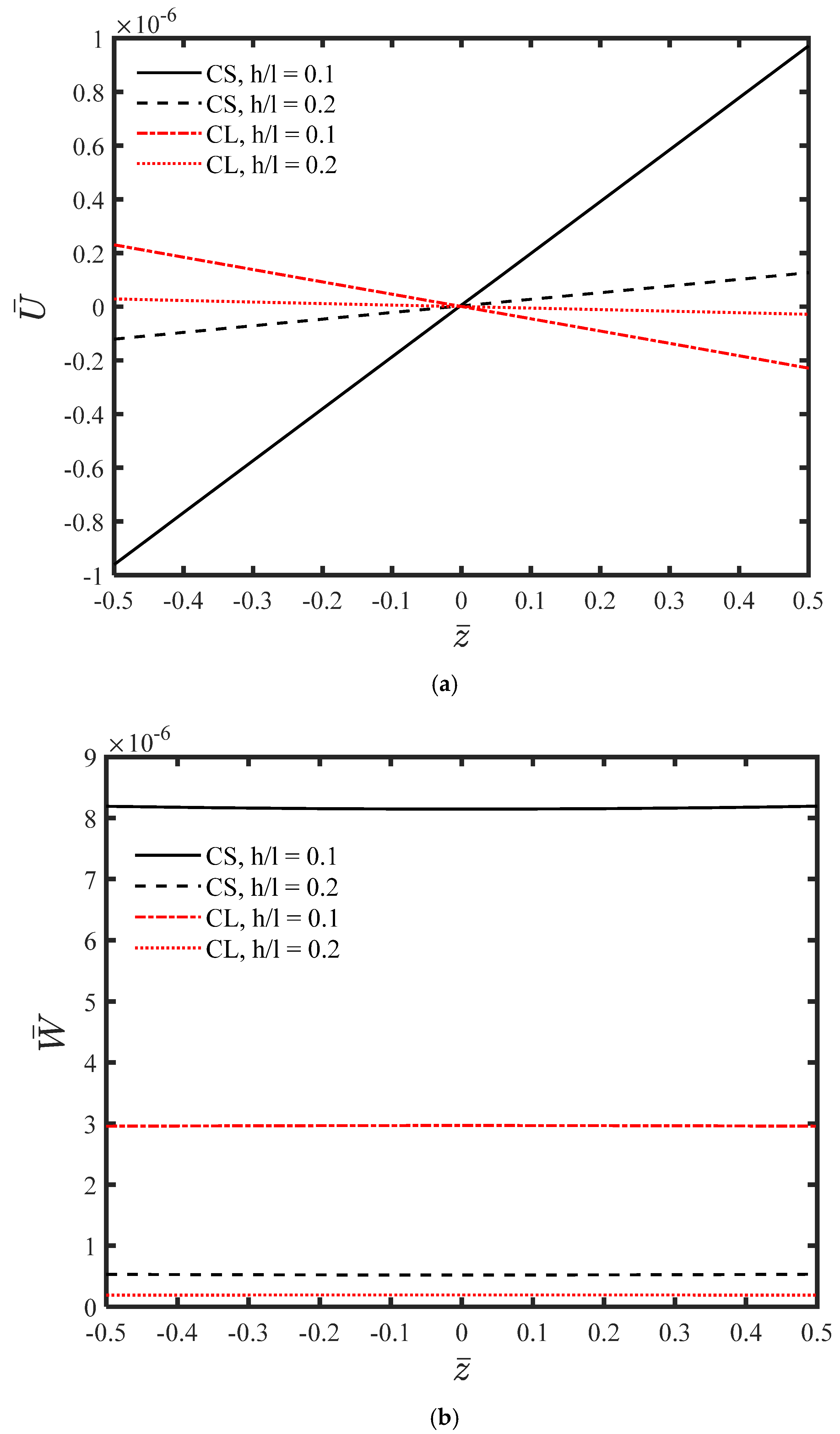
The absolute values of displacements decrease as the thickness of the microplate increases.

4-

For a constant h/l ratio, the displacements calculated using couple stress theory are greater than those predicted by classical theory.

5-

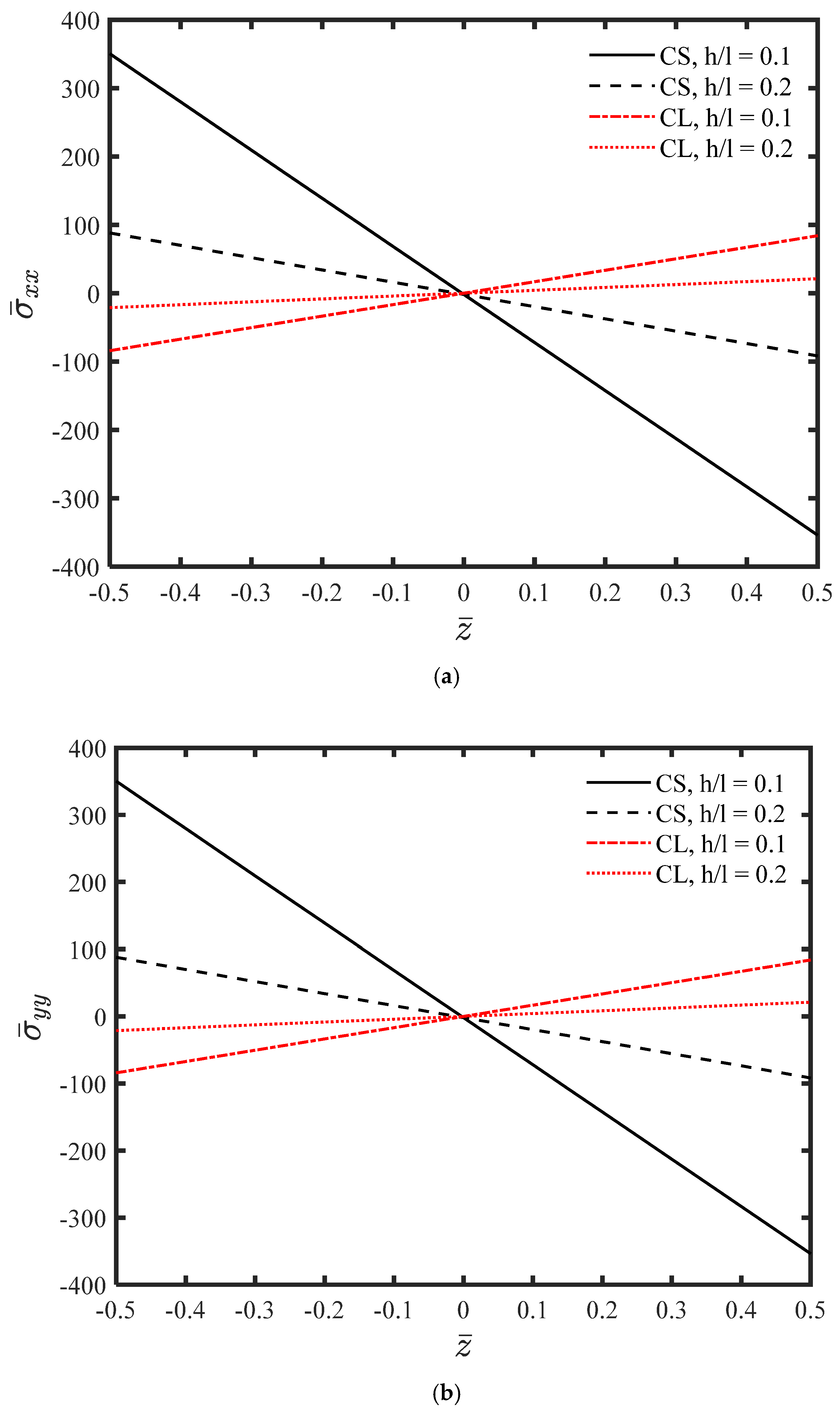
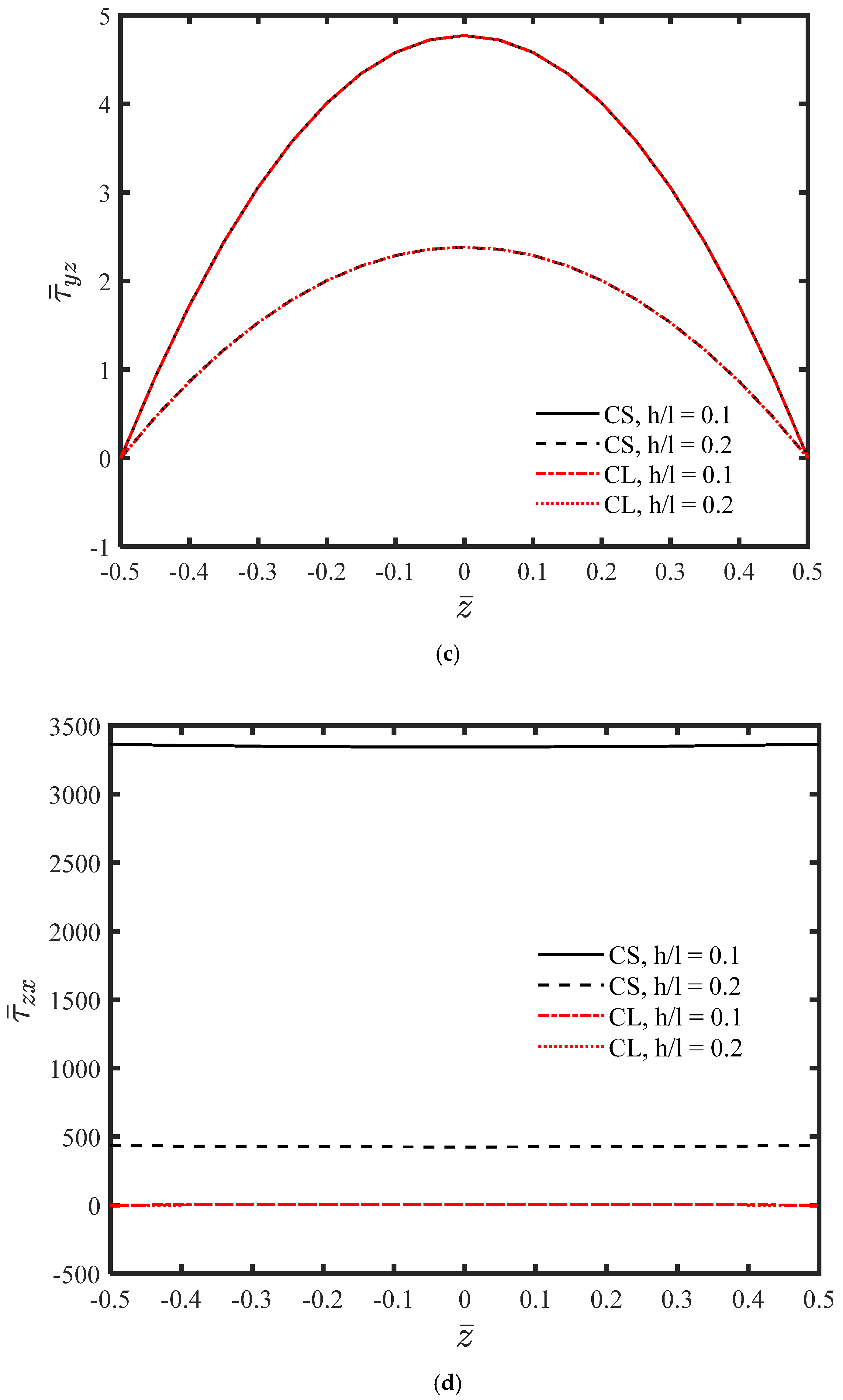
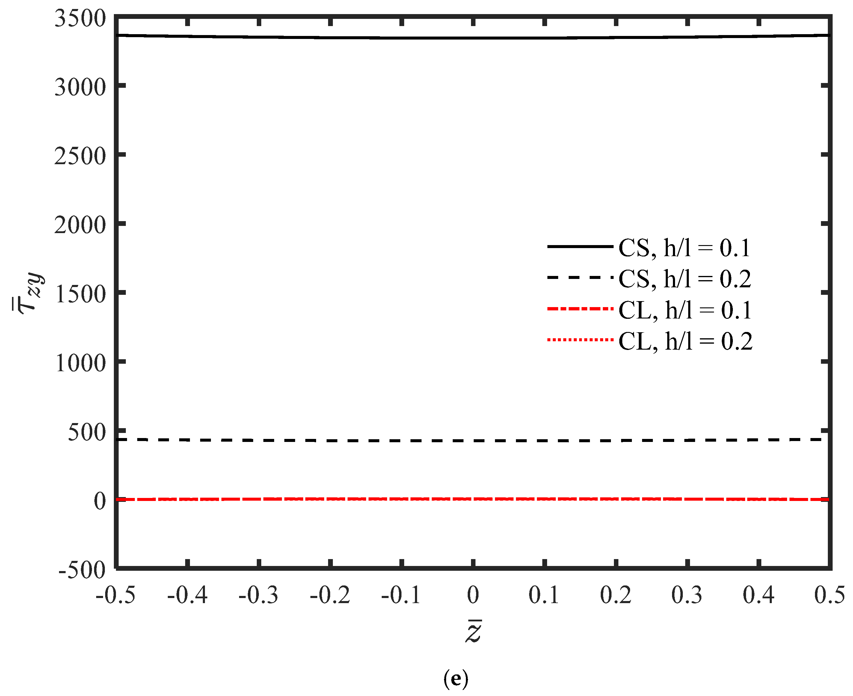
As the thickness of the microplate increases, the absolute values of stresses decrease.

6-

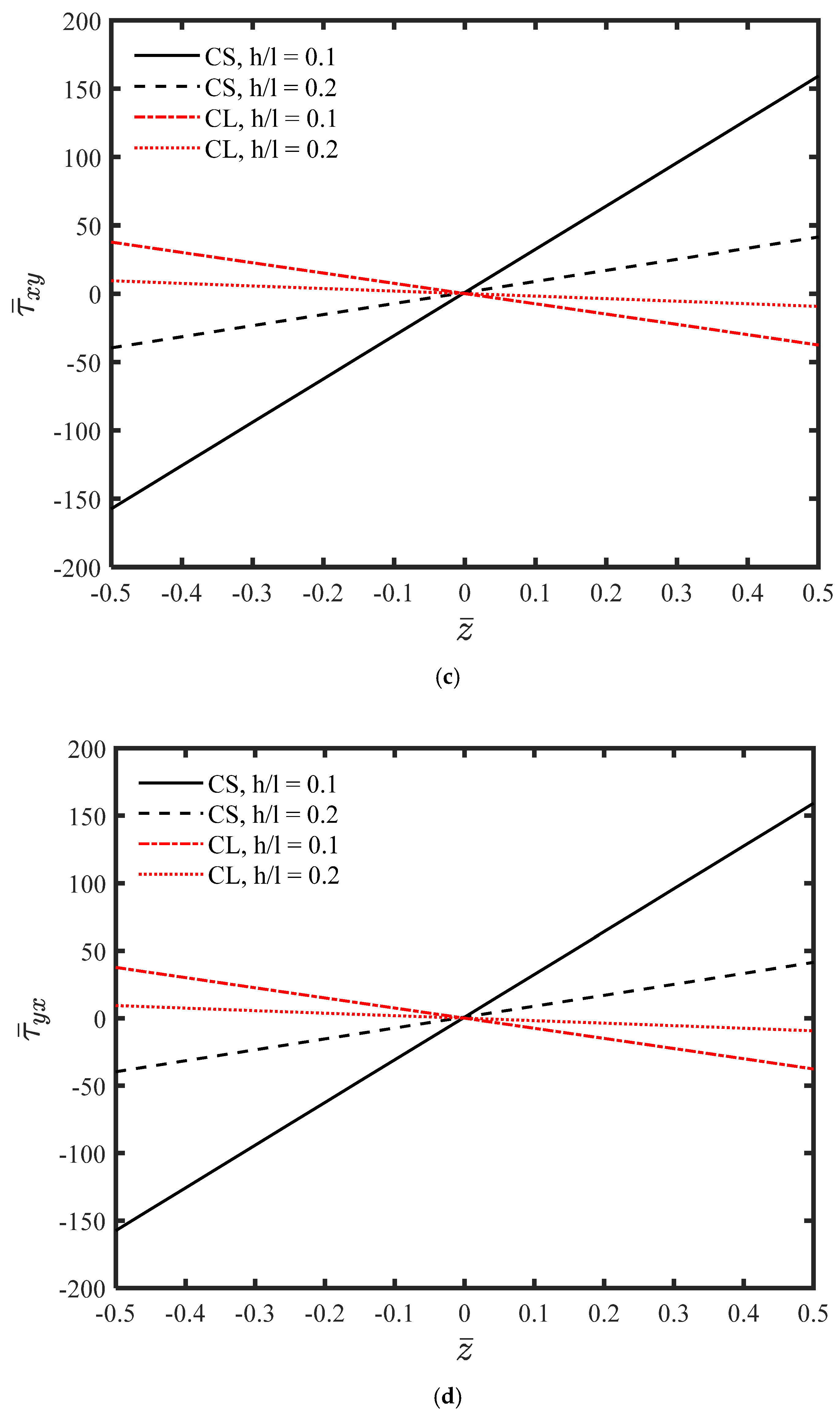
Unlike classical theories, ${\overline{\tau }}_{ij}$ and ${\overline{\tau }}_{ji}$ are not identical.

7-

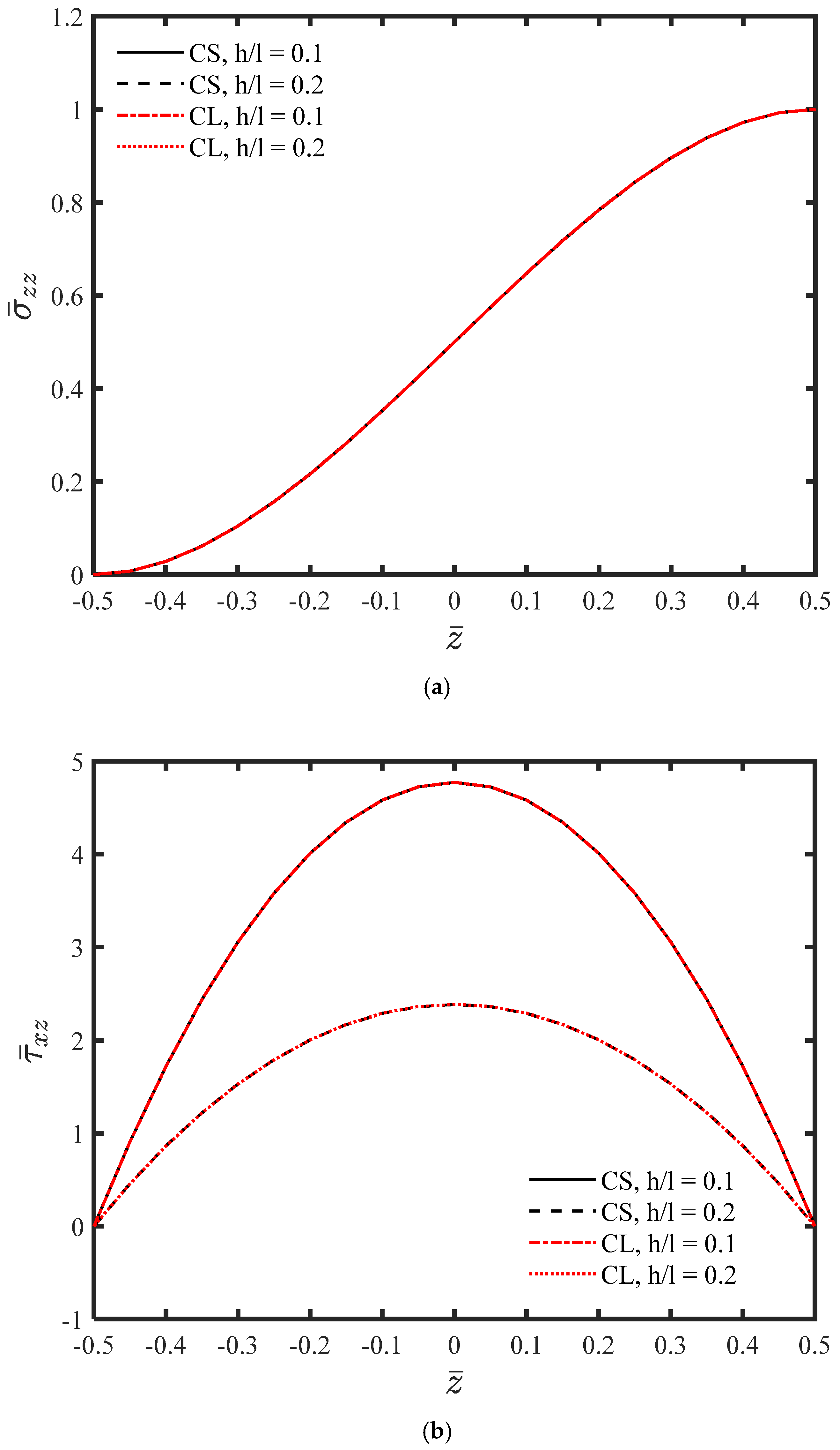
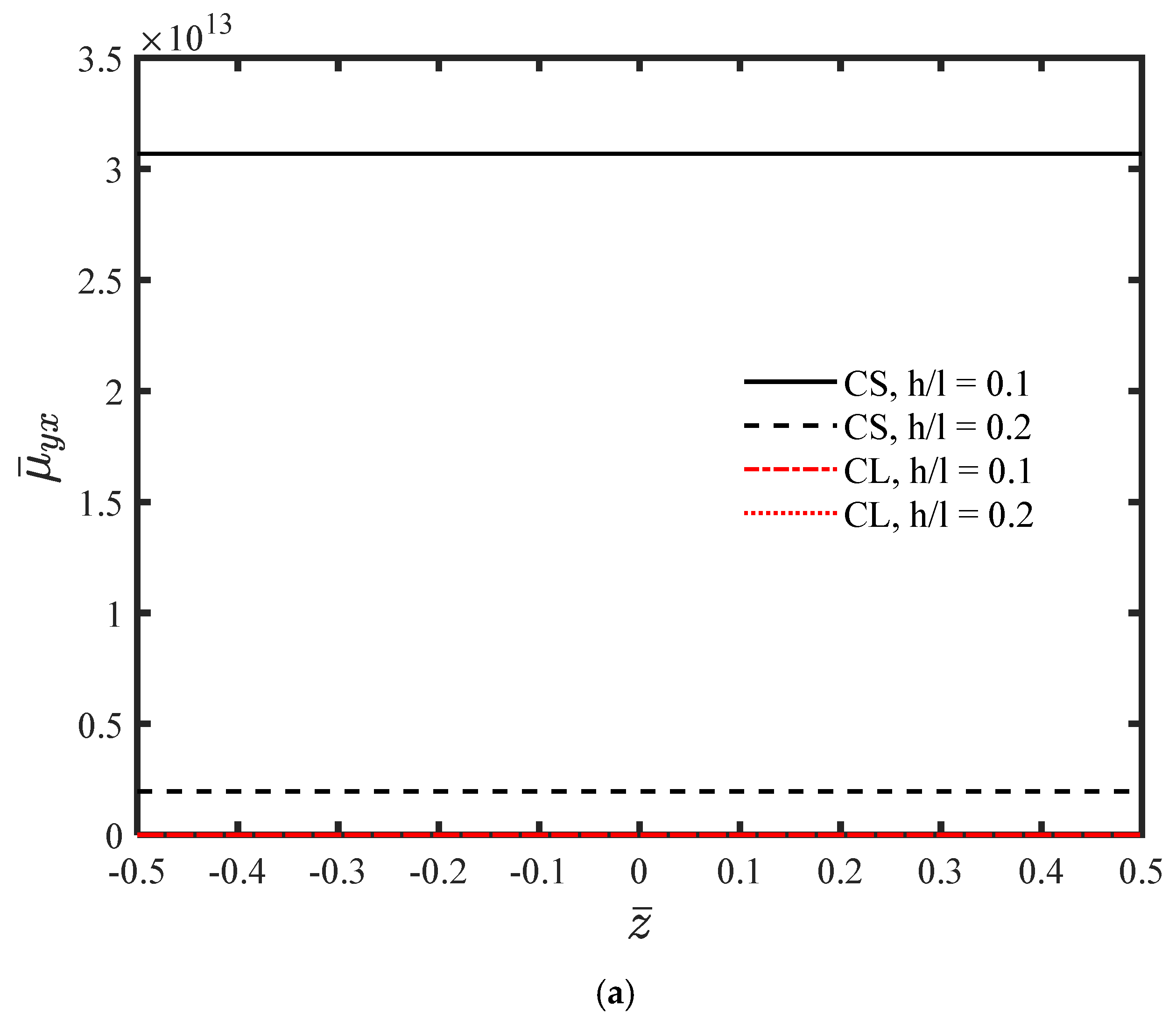
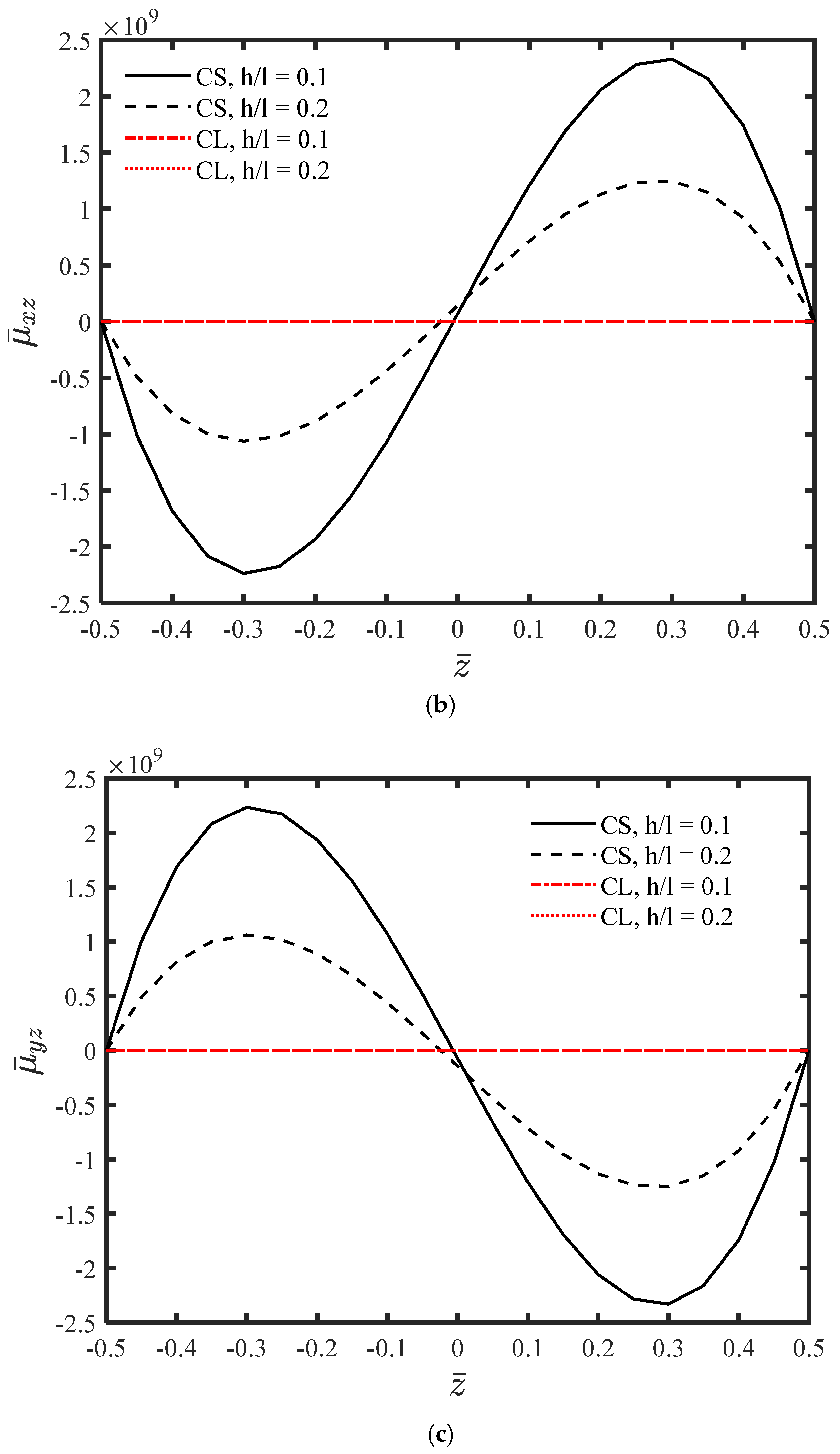
Compared to classical elasticity theory, the out-of-plane stresses attain larger values, and these components increase further as the thickness decreases.

8-

An increase in thickness results in a reduction in the absolute value of ${\overline{\mu }}_{ij}$.

References

- Mcfarland, A.W.; Colton, J.S. Role of material microstructure in plate stiffness with relevance to microcantilever sensors. J. Micromech. Microeng. 2005, 15, 1060–1067. [Google Scholar] [CrossRef]
- Lei, J.; He, Y.; Guo, S.; Li, Z.; Liu, D. Size-dependent vibration of nickel cantilever microbeams: Experiment and gradient elasticity. AIP Adv. 2016, 6, 105202. [Google Scholar] [CrossRef]
- Kandaz, M.; Dal, H. A comparative study of modified strain gradient theory and modified couple stress theory for gold microbeams. Arch. Appl. Mech. 2018, 88, 2051–2070. [Google Scholar] [CrossRef]
- Shaban, M.; Mazaheri, H. Size-dependent electro-static analysis of smart micro-sandwich panels with functionally graded core. Acta Mech. 2020, 232, 111–133. [Google Scholar] [CrossRef]
- Dastjerdi, S.; Akgöz, B. New static and dynamic analyses of macro and nano FGM plates using exact three-dimensional elasticity in thermal environment. Compos. Struct. 2018, 192, 626–641. [Google Scholar] [CrossRef]
- Ansari, R.; Norouzzadeh, A.; Shakouri, A.H.; Bazdid-Vahdati, M.; Rouhi, H. Finite element analysis of vibrating micro-beams and -plates using a three-dimensional micropolar element. Thin-Walled Struct. 2018, 124, 489–500. [Google Scholar] [CrossRef]
- Mindlin, R.D.; Tiersten, H.F. Effects of couple-stresses in linear elasticity. Arch. Ration. Mech. Anal. 1962, 11, 415–448. [Google Scholar] [CrossRef]
- Mindlin, R.D.; Eshel, N.N. On first strain-gradient theories in linear elasticity. Int. J. Solids Struct. 1968, 4, 109–124. [Google Scholar] [CrossRef]
- Yang, F.; Chong, A.C.M.; Lam, D.C.C.; Tong, P. Couple stress based strain gradient theory for elasticity. Int. J. Solids Struct. 2002, 39, 2731–2743. [Google Scholar] [CrossRef]
- Park, S.K.; Gao, X.L. Bernoulli-Euler beam model based on a modified couple stress theory. J. Micromech. Microeng. 2006, 16, 2355–2359. [Google Scholar] [CrossRef]
- Asghari, M.; Ahmadian, M.T.; Kahrobaiyan, M.H.; Rahaeifard, M. On the size-dependent behavior of functionally graded micro-beams. Mater. Des. 2010, 31, 2324–2329. [Google Scholar] [CrossRef]
- Reddy, J.N. Microstructure-dependent couple stress theories of functionally graded beams. J. Mech. Phys. Solids 2011, 59, 2382–2399. [Google Scholar] [CrossRef]
- Gao, X.L.; Mahmoud, F.F. A new Bernoulli-Euler beam model incorporating microstructure and surface energy effects. Z. Angew. Math. Phys. 2014, 65, 393–404. [Google Scholar] [CrossRef]
- Sßimsßek, M.; Reddy, J.N. Bending and vibration of functionally graded microbeams using a new higher order beam theory and the modified couple stress theory. Int. J. Eng. Sci. 2013, 64, 37–53. [Google Scholar] [CrossRef]
- Jabbari Behrouz, S.; Rahmani, O.; Hosseini, S.A. On nonlinear forced vibration of nano cantilever-based biosensor via couple stress theory. Mech. Syst. Signal Process. 2019, 128, 19–36. [Google Scholar] [CrossRef]
- Gan, N.; Wang, Q. Topology optimization design for buckling analysis related to the size effect. Math. Mech. Solids 2021, 27, 10812865211066608. [Google Scholar] [CrossRef]
- Reddy, J.N.; Berry, J. Nonlinear theories of axisymmetric bending of functionally graded circular plates with modified couple stress. Compos. Struct. 2012, 94, 3664–3668. [Google Scholar] [CrossRef]
- Tsiatas, G.C. A new Kirchhoff plate model based on a modified couple stress theory. Int. J. Solids Struct. 2009, 46, 2757–2764. [Google Scholar] [CrossRef]
- Ashoori, A.R.; Sadough Vanini, S.A. Thermal buckling of annular microstructure-dependent functionally graded material plates resting on an elastic medium. Compos. Part B Eng. 2016, 87, 245–255. [Google Scholar] [CrossRef]
- Ashoori, A.R.; Sadough Vanini, S.A. Nonlinear thermal stability and snap-through behavior of circular microstructure-dependent FGM plates. Eur. J. Mech. A/Solids 2016, 59, 323–332. [Google Scholar] [CrossRef]
- Beni, Y.T.; Mehralian, F.; Zeighampour, H. The modified couple stress functionally graded cylindrical thin shell formulation. Mech. Adv. Mater. Struct. 2016, 23, 791–801. [Google Scholar] [CrossRef]
- Ma, H.M.; Gao, X.L.; Reddy, J.N. A non-classical Mindlin plate model based on a modified couple stress theory. Acta Mech. 2011, 220, 217–235. [Google Scholar] [CrossRef]
- Alinaghizadeh, F.; Shariati, M.; Fish, J. Bending analysis of size-dependent functionally graded annular sector microplates based on the modified couple stress theory. Appl. Math. Model. 2017, 44, 540–556. [Google Scholar] [CrossRef]
- Jung, W.Y.; Han, S.C. Static and eigenvalue problems of Sigmoid Functionally Graded Materials (S-FGM) micro-scale plates using the modified couple stress theory. Appl. Math. Model. 2015, 39, 3506–3524. [Google Scholar] [CrossRef]
- Eshraghi, I.; Dag, S.; Soltani, N. Consideration of spatial variation of the length scale parameter in static and dynamic analyses of functionally graded annular and circular micro-plates. Compos. Part B Eng. 2015, 78, 338–348. [Google Scholar] [CrossRef]
- Eshraghi, I.; Dag, S.; Soltani, N. Bending and free vibrations of functionally graded annular and circular micro-plates under thermal loading. Compos. Struct. 2016, 137, 196–207. [Google Scholar] [CrossRef]
- Ghayesh, M.H.; Farokhi, H. Coupled size-dependent behavior of shear deformable microplates. Acta Mech. 2016, 227, 757–775. [Google Scholar] [CrossRef]
- Chen, W.; Li, X. A new modified couple stress theory for anisotropic elasticity and microscale laminated Kirchhoff plate model. Arch. Appl. Mech. 2014, 84, 323–341. [Google Scholar] [CrossRef]
- He, D.; Yang, W.; Chen, W. A size-dependent composite laminated skew plate model based on a new modified couple stress theory. Acta Mech. Solida Sin. 2017, 30, 75–86. [Google Scholar] [CrossRef]
- Li, Q.; Niu, X.; Pan, Z. Size-dependent effects of graded porous micro-/nanocircular plates on thermal vibration based on modified couple stress theory. Mech. Based Des. Struct. Mach. 2025, 1–27. [Google Scholar] [CrossRef]
- Hadjesfandiari, A.R.; Dargush, G.F. Couple stress theory for solids. Int. J. Solids Struct. 2011, 48, 2496–2510. [Google Scholar] [CrossRef]
- Hadjesfandiari, A.R. Size-dependent piezoelectricity. Int. J. Solids Struct. 2013, 50, 2781–2791. [Google Scholar] [CrossRef]
- Alashti, R.A.; Abolghasemi, A.H. A Size-dependent Bernoulli-Euler Beam Formulation based on a New Model of Couple Stress Theory. Int. J. Eng. 2014, 27, 951–960. [Google Scholar] [CrossRef]
- Fakhrabadi, M.M.S.; Yang, J. Comprehensive nonlinear electromechanical analysis of nanobeams under DC/AC voltages based on consistent couple-stress theory. Compos. Struct. 2015, 132, 1206–1218. [Google Scholar] [CrossRef]
- Seyyed Fakhrabadi, M.M. Prediction of small-scale effects on nonlinear dynamic behaviors of carbon nanotube-based nano-resonators using consistent couple stress theory. Compos. Part B Eng. 2016, 88, 26–35. [Google Scholar] [CrossRef]
- Hadjesfandiari, A.R.; Dargush, G.F. Comparison of theoretical elastic couple stress predictions with physical experiments for pure torsion. arXiv 2016, arXiv:1605.02556, 1–25. [Google Scholar]
- Tadi Beni, Y. Size-dependent electromechanical bending, buckling, and free vibration analysis of functionally graded piezoelectric nanobeams. J. Intell. Mater. Syst. Struct. 2016, 27, 2199–2215. [Google Scholar] [CrossRef]
- Keivani, M.; Koochi, A.; Abadyan, M. A new model for stability analysis of electromechanical nano-actuator based on Gurtin-Murdoch and consistent couple-stress theories. J. Vibroeng. 2016, 18, 1406–1416. [Google Scholar] [CrossRef]
- Nejad, M.Z.; Hadi, A.; Farajpour, A. Consistent couple-stress theory for free vibration analysis of Euler-Bernoulli nano-beams made of arbitrary bi-directional functionally graded materials. Struct. Eng. Mech. 2017, 63, 161–169. [Google Scholar] [CrossRef]
- Hadjesfandiari, A.R.; Hajesfandiari, A.; Zhang, H.; Dargush, G.F. Size-dependent couple stress Timoshenko beam theory. arXiv 2017, arXiv:1712.08527, 1–48. [Google Scholar]
- Fattahian Dehkordi, S.; Tadi Beni, Y. Electro-mechanical free vibration of single-walled piezoelectric/flexoelectric nano cones using consistent couple stress theory. Int. J. Mech. Sci. 2017, 128–129, 125–139. [Google Scholar] [CrossRef]
- Ajri, M.; Fakhrabadi, M.M.S.; Rastgoo, A. Analytical solution for nonlinear dynamic behavior of viscoelastic nano-plates modeled by consistent couple stress theory. Lat. Am. J. Solids Struct. 2018, 15, 1–23. [Google Scholar] [CrossRef]
- Amin Hadi, M.Z.N.; Rastgoo, A.; Hosseini, M. Buckling analysis of FGM Euler-Bernoulli nano-beams with 3D-varying properties based on consistent couple-stress theory. Steel Compos. Struct. 2018, 26, 663–672. [Google Scholar] [CrossRef]
- Wu, C.-P.; Hu, H.-X. A unified size-dependent plate theory for static bending and free vibration analyses of micro- and nano-scale plates based on the consistent couple stress theory. Mech. Mater. 2021, 162, 104085. [Google Scholar] [CrossRef]
- Kutbi, M.A.; Zenkour, A.M. Modified couple stress model for thermoelastic microbeams due to temperature pulse heating. J. Comput. Appl. Mech. 2022, 53, 83–101. [Google Scholar] [CrossRef]
- Zhang, R.; Bai, H.; Chen, X. The Consistent Couple Stress Theory-Based Vibration and Post-Buckling Analysis of Bi-directional Functionally Graded Microbeam. Symmetry 2022, 14, 602. [Google Scholar] [CrossRef]
- Wu, C.P.; Lyu, Y.S. An asymptotic consistent couple stress theory for the three-dimensional free vibration analysis of functionally graded microplates resting on an elastic medium. Math. Methods Appl. Sci. 2023, 46, 4891–4919. [Google Scholar] [CrossRef]
- Wu, C.P.; Huang, Z. A unified consistent couple stress beam theory for functionally graded microscale beams. Steel Compos. Struct. 2024, 51, 103–116. [Google Scholar] [CrossRef]
- Huang, H.; Guan, W.; He, X. Modal displacement analyses of Lamb waves in micro/nano-plates based on the consistent couple stress theory. Ultrasonics 2024, 138, 107272. [Google Scholar] [CrossRef]
- Wu, C.P.; Lu, Y.A. 3D static bending analysis of functionally graded piezoelectric microplates resting on an elastic medium subjected to electro-mechanical loads using a size-dependent Hermitian C2 finite layer method based on the consistent couple stress theory. Mech. Based Des. Struct. Mach. 2024, 52, 3799–3841. [Google Scholar] [CrossRef]
- Shang, Y.; Sun, M.; Cen, S.; Li, C.F. Computational homogenization of flexoelectric composites within the consistent couple stress theory. Comput. Methods Appl. Mech. Eng. 2025, 437, 117762. [Google Scholar] [CrossRef]
- Sadd, M.H. Elasticity: Theory, Applications, and Numerics, 3rd ed.; Academic Press: Cambridge, MA, USA, 2014; ISBN 9780124081369. [Google Scholar] [CrossRef]
- Hadjesfandiari, A.R.; Dargush, G.F. Fundamental solutions for isotropic size-dependent couple stress elasticity. Int. J. Solids Struct. 2013, 50, 1253–1265. [Google Scholar] [CrossRef]
- Shaban, M. Elasticity Solution for Static Analysis of Sandwich Structures with Sinusoidal Corrugated Cores. J. Stress Anal. 2016, 1, 23–31. [Google Scholar]
- Pagano, N.J. Exact Solutions for Rectangular Bidirectional Composites and Sandwich Plates. J. Compos. Mater. 1970, 4, 20–34. [Google Scholar] [CrossRef]