Hierarchical Free Vibration Analysis of Variable-Angle Tow Shells Using Unified Formulation

Abstract

This paper investigates the dynamic behavior of shell structures presenting variable-angle tow laminations. The choice of placing fibers along curvilinear patterns allows for a broader structural design space, which is advantageous in several engineering contexts, provided that more complex numerical analyses are managed. In this regard, Carrera’s unified formulation has been widely used for studying variable-angle tow plates and shells. This article aims to expand this formulation through the derivation of the complete formulation for a generic shell reference surface. The principle of virtual displacements is used as a variational statement for obtaining, in a weak sense, the stiffness and mass matrices within the finite element solution method. The free vibration problem of singly and doubly curved variable-angle tow shells is then addressed. The proposed approach is compared to Abaqus three-dimensional reference solutions and classical theories to investigate the effectiveness of the developed models in predicting the vibrational frequencies and modes. The results demonstrate a good agreement between the proposed approach and reference solutions.

1. Introduction

The study of shell structures has significantly expanded in recent decades. Composite shells, in particular, have been utilized across various engineering contexts due to their excellent mechanical properties and low weight. The versatility and efficiency of shell structures make them an ideal choice for a wide range of applications, including aerospace and civil engineering and the automotive industry, as well as several other industrial fields. On the other hand, shell theory is more complicated than classical plate theories because the middle surface curvature generates more complex equations of motion. Thanks to the development of new manufacturing technologies, variable-angle tow (VAT) composites can be arranged in shell configurations in order to further improve the mechanical properties of these structures. Among the various processes used for manufacturing VAT composites, automated fiber placement (AFP) and modern 3D printing (3DP) techniques play a pivotal role. AFP allows one to place prepreg composite materials onto a mold or mandrel. Usually, this technique uses a robotic arm that moves the placement head through a predefined path. When the tow lays down along a straight path, conventional composites can be obtained. During the process, a heating system allows one to obtain a tacky resin, which is compressed on the surface to avoid gaps. The choice of the material is crucial and can heavily influence the final overall quality. Three kinds of materials are typically used for the AFP process: thermosets, thermoplastics and dry fibers. The term “prepreg” refers to thermosets and thermoplastics, since the fibers are already pre-impregnated with resin while dry fibers are not. More details about AFP techniques can be found in the work by Brasington et al. [1]. The manufacturing technique strongly influences the actual placement of fibers and the presence of gaps/overlaps. For example, the standard AFP head operates by rotating to ensure that the compaction roller remains perpendicular to the tangent of the reference tow path. During this process, the tow material is deposited by relying on its in-plane bending deformation. However, this can lead to fiber buckling on the inner side and straightening on the outer side of the curved tow path. This kind of problematic is further discussed by Kim, Potter and Weaver [2], who proposed an alternative method called continuous tow shearing (CTS). Three-dimensional printing techniques appear to be very promising in the context of composite manufacturing because of the possibility to represent complex geometries, and offer cost-effective solutions for small-scale production. For example, fusion deposition modeling (FDM) is a process where the material is extruded from a nozzle, enabling the formation of layers. Usually, these kinds of processes use thermoplastic polymers and the fiber reinforcements are constrained by the size of the nozzle. The printing process uses materials that are commonly used for conventional composites, including carbon fibers, glass fibers, Kevlar and natural fibers. More details about the kinds of materials that can be considered within this type of process can be found in the work by Zhuo et al. [3]. Various engineering applications can benefit from the use of VAT composites. For example, Brooks et al. [4] used these materials for aircraft wings to optimize the structural weight and fuel consumption. VATs can also be applied in the aerospace context for air launch vehicle applications as discussed by Grenoble et al. [5]. By placing fibers along curvilinear patterns, it is possible to enhance the stiffness of classical composites. In a more generic view, this leads to a wider structural design space and a broader tailoring choice for various kinds of problems. For example, it can be useful to orient the fibers along specific patterns to improve the search for an optimal solution within an optimization context. This can also be convenient when the analyzed structure presents geometrical discontinuities such as cut-outs. One of the main disadvantages of VATs is the increased complexity of analysis. This is due to the greater number of unknown variables that need to be considered, which can lead to fiber patterns during the optimization process that cannot be actually manufactured. The combination of complexities related to shell geometry and VAT composites highlights the necessity of accurate yet computationally efficient numerical tools for the mechanical investigation of VAT shells.

Various methods have been employed for such analyses. Some of these approaches are briefly discussed in the following text to establish the foundational basis upon which the proposed work is developed. The theoretical concept of shell structures is quite old and has been developed under various theories over the last century. Love [6] provided a general overview of plate vibration and flexure theories, followed by their extension to the case of shells. Additionally, Donnell [7] proposed an exact solution to study the stability of cylindrical walls, demonstrating that experimentally obtained buckling loads are smaller than theoretical ones. A fundamental contribution in shell theory was given by Flügge [8], who studied the distribution of stresses in shells considering several geometries, loads and boundary conditions. Among the various techniques that were used to study shells structures, the finite element method (FEM) has been instrumental in advancing this field. A general overview of the application of the FEM to shells was given by Lindberg, Olson and Cowper [9]. As stated in their work, two approaches can be followed to predict shells’ mechanical behavior through the FEM. The former is based on the idea of using flat elements to discretize a curved surface. This method was followed by Clough and Johnson [10], who performed a static analysis of shell structures through flat triangular elements. The second possible approach consists of developing curved shell elements that allow one to better approximate the geometry of the analyzed structure. As an example of this latter approach, Bogner, Fox and Schmit [11] proposed a cylindrical element to perform a static analysis of a pinched cylinder. The multiple attempts to develop a quadrilateral shell element showed that, in most cases, the elements resulted in excessive stiffness. This happens because of the combination of shear and membrane locking that usually characterizes these elements [12]. Bathe and Dvorkin [13] developed reliable shell elements with four and eight nodes through the use of a mixed interpolation of tensorial components. Subsequently, the same approach was extended by Bucalem and Bathe [14] to elements with nine and sixteen nodes. Among the several theories developed in the context of structural mechanics, Carrera’s unified formulation (CUF) has shown good results while maintaining a reasonable computational cost. According to CUF, the preliminary choice of expansion functions along the thickness allows one to obtain a wide family of hierarchic theories within a unique formulation (see Carrera [15]). CUF was initially applied to shell structures through a Navier-type closed-form solution. This approach was used by Carrera et al. [16] to perform a free vibration analysis of cylindrical and spherical shells. Giunta et al. [17] used the same method in a static analysis context. Subsequently, CUF was extended to thermo-mechanical analyses as shown by Giunta et al. [18]. In this work, isotropic and composite beams subjected to thermal loads were studied, utilizing a meshless collocation method with Wendland’s radial basis functions. Brischetto, Polit and Carrera [19] proposed an eight-node element with nine degrees of freedom per node to contrast the shear and membrane locking phenomena. Cinefra and Carrera [20] extended the use of CUF to a static analysis of cylindrical structures in the FEM context. Cinefra, Chinosi and Della Croce [21] investigated the performance of the proposed nine-node shell element through a static analysis of classical problems like the pinched shell and the Scordelis–Lo roof. Cinefra, Kumar and Carrera [22] introduced Reissner’s mixed variational theorem within CUF shell elements to perform static analyses. Kumar et al. [23] performed a free vibration analysis of doubly curved shells subjected to delamination. Shells of revolution were studied through CUF by Carrera and Zozulya [24,25,26]. An important contribution in shell theory was given by Tornabene, Liverani and Caligiana [27], who applied the generalized differential quadrature (GDQ) method with the first-order shear deformation theory for a free vibration analysis of anisotropic shells of revolution. Subsequently, this approach was extended to CUF by Tornabene et al. [28] for a static analysis of doubly curved shells.

The potential for placing fibers along curvilinear paths within a shell structural domain is promising for enhancing the mechanical properties of a composite. As shown by Wu et al. [29], new manufacturing technologies could efficiently integrate the VAT concept within a shell geometry. To the best of the authors’ knowledge, Hyer and Charette [30] were among the pioneers in introducing the VAT concept. In their work, they utilized the finite element method (FEM) to model the variation in the path of continuous fibers, assuming a constant fiber angle within each finite element. In some more recent developments, Tornabene, Fantuzzi and Bacciocchi [31] used CUF for the static analysis of curvilinear fibers shells, and the numerical problems were solved through the GDQ method. Sánchez-Majano et al. [32] studied the static behavior of VAT cylindrical shells through CUF. Sciascia et al. [33] studied VAT shells considering buckling, free vibrations and prestressed vibrations. A seven-parameter shell formulation was used within the principle of virtual work to obtain an equivalent single-layer model for the VAT cylindrical shells stability study by He et al. [34]. Numerous studies have demonstrated that utilizing curvilinear fibers can increase the fundamental frequency. For example, Blom et al. [35] maximized the first natural frequency of VSC conical shells, considering manufacturing constraints. Carvalho, Sohouli et al. [36] used a genetic algorithm and shell elements based on first-order shear deformation theory for the maximization of the fundamental frequency. Among the various optimization methods that could be applied to VAT structures, the multi-scale two-level (MS2L) approach stands out for its ability to efficiently handle complex designs by simultaneously considering global and local optimization criteria. This method divides the optimization process into two distinct phases. Initially, the composite is represented as a homogeneous anisotropic plate to determine the optimal distribution of polar parameters, which are the mechanical design variables. In the subsequent phase, the focus shifts to determining the optimal stacking sequence based on the mechanical properties distribution derived from the first phase. More details about the MS2L approach can be found in the studies by Catapano et al. [37], Montemurro and Catapano [38,39] and Fiordilino et al. [40], where both stiffness and buckling optimization problems were solved.

Despite the large amount of articles that have been published on shells, the literature regarding the application of CUF to the free vibration analysis of VAT shells of revolution offers some room for contributions. Toward this end, this article presents a new development of CUF for the dynamic study of curvilinear fiber shells with single and double curvature. Specifically, this work extends the proposed approach to surfaces with non-constant coefficients of the first quadratic form, enabling the consideration of more complex shell geometries. The structure of this paper is as follows. Section 2 introduces the CUF approach and demonstrates its application to VAT shells using a pure displacement formulation. Section 3 considers two cylindrical shells and a spherical segment in order to perform an eigenvalue free vibration analysis considering various boundary conditions. The results are compared with reference solutions obtained in Abaqus using three-dimensional (3D) elements. Finally, Section 4 shows the conclusive remarks.

2. Carrera’s Unified Formulation

Shells are 3D objects defined by two closely spaced surfaces with the distance between them significantly smaller than the other dimensions of the shell. The set of midpoints between these surfaces forms the middle surface of the shell. The thickness of the shell at any point is the distance between the surfaces measured along a normal to the middle surface at that point. In order to formulate the shell kinematics, a curvilinear reference system is considered: $\alpha$ and $\beta$ are curvilinear axes that lay on the shell mid-surface, while the through-the-thickness axis (or z-axis) is oriented along the thickness of the shell. The thickness dimension is indicated as h, while $l_{\alpha }$ and $l_{\beta }$ refer to the characteristics lengths along $\alpha$ and $\beta$ axes, respectively. The mathematical description of the shell starts from the definition of the radius vector, which points at the undeformed middle surface of the shell, starting from a global Cartesian reference system defined by X, Y and Z axes (as shown in Figure 1):

$$\mathbf{r}=\mathbf{r}\left(\alpha ,\beta \right).$$

(1)

The infinitesimal variation in the vector $\mathbf{r}$ can be defined as

$$d\mathbf{r}=\mathbf{r}{,}_{\alpha }d\alpha +\mathbf{r}{,}_{\beta }d\beta ,$$

(2)

where subscripts preceded by a comma refer to the derivative along the curvilinear reference system axes. The norms of the derivative vectors can be expressed as

$$\begin{array}{c}\left|\mathbf{r}{,}_{\alpha }\right|=A,\hfill \\ \left|\mathbf{r}{,}_{\beta }\right|=B,\hfill \end{array}$$

(3)

where $\left|\square \right|$ is a vector norm operator. The following unit vectors are introduced:

$$\begin{array}{c}{\mathbf{i}}_{\alpha }=\mathbf{r}{,}_{\alpha }/A,\hfill \\ {\mathbf{i}}_{\beta }=\mathbf{r}{,}_{\beta }/B,\hfill \\ {\mathbf{i}}_n={\mathbf{i}}_{\alpha }\times {\mathbf{i}}_{\beta }/sin\left(\chi \right),\hfill \end{array}$$

(4)

where ${\mathbf{i}}_{\alpha }$ and ${\mathbf{i}}_{\beta }$ are the unit tangent vectors along $\alpha$ and $\beta$ axes, respectively. By its definition, ${\mathbf{i}}_n$ is the unit vector along the thickness and is orthogonal to both ${\mathbf{i}}_{\alpha }$ and ${\mathbf{i}}_{\beta }$, being × the vector cross product operator. The angle between the mid-surface axes $\alpha$ and $\beta$ is indicated as $\chi$. The first quadratic form of the surface corresponds to the right-hand side of the following equation:

$$d\mathbf{r}·d\mathbf{r}=A^{2}d{\alpha }^2+2ABcos\left(\chi \right)d\alpha d\beta +B^{2}d{\beta }^2,$$

(5)

where · is vector scalar product operator. The second quadratic form is related to the problem of finding the curvature of a generic curve on a surface. For the sake of brevity, only the final formula of the normal curvature of the surface is presented:

$${\displaystyle \frac{1}{R}}=-{\displaystyle \frac{Ld{\alpha }^2+2Md\alpha d\beta +Nd{\beta }^2}{A^{2}d{\alpha }^2+2ABcos\left(\chi \right)d\alpha d\beta +B^{2}d{\beta }^2}},$$

(6)

where the numerator of the right-hand side of the equation is the second quadratic form of a surface. The following terms are also introduced:

$$\begin{array}{c}L=\mathbf{r}{,}_{\alpha \alpha }{\mathbf{i}}_n,\hfill \\ M=\mathbf{r}{,}_{\alpha \beta }{\mathbf{i}}_n,\hfill \\ N=\mathbf{r}{,}_{\beta \beta }{\mathbf{i}}_n.\hfill \end{array}$$

(7)

The curvatures of $\alpha$ and $\beta$ lines can be obtained by considering $\beta$ and $\alpha$ as constants, respectively:

$$\begin{array}{c}{\displaystyle \frac{1}{R_{\alpha }}}=-{\displaystyle \frac{L}{A^2}},\hfill \\ {\displaystyle \frac{1}{R_{\beta }}}=-{\displaystyle \frac{N}{B^2}}.\hfill \end{array}$$

(8)

The assumption that $\alpha$ and $\beta$ are lines of principal curvature of the surface allows one to simplify the shell equations. It can be shown that the necessary and sufficient conditions for $\alpha$ and $\beta$ to be lines of principal curvature are as follows:

$$\begin{array}{c}cos\left(\chi \right)=0,\hfill \\ M=0.\hfill \end{array}$$

(9)

The location of a generic point within the shell domain can be written as

$$\mathbf{R}\left(\alpha ,\beta ,z\right)=\mathbf{r}\left(\alpha ,\beta \right)+z{\mathbf{i}}_n\left(\alpha ,\beta \right).$$

(10)

The square of the modulus of an infinitesimal change in the $\mathbf{R}$ vector can be written as follows:

$$d\mathbf{R}·d\mathbf{R}=\left(d\mathbf{r}+zd{\mathbf{i}}_n+{\mathbf{i}}_{n}dz\right)\left(d\mathbf{r}+zd{\mathbf{i}}_n+{\mathbf{i}}_{n}dz\right)=H_{\alpha }^{2}d{\alpha }^2+H_{\beta }^{2}d{\beta }^2+H_z^{2}d{z}^2,$$

(11)

where

$$\begin{array}{c}{H}_{\alpha }=A\left(1+z/R_{\alpha }\right),\hfill \\ H_{\beta }=B\left(1+z/R_{\beta }\right),\hfill \\ H_z=1.\hfill \end{array}$$

(12)

Subsequently, the infinitesimal surface and volume of the fundamental shell element can be written as

$$\begin{array}{c}d\mathrm{\Omega }=H_{\alpha }{H}_{\beta }d\alpha d\beta ,\hfill \\ dV=H_{\alpha }{H}_{\beta }{H}_{z}d\alpha d\beta dz.\hfill \end{array}$$

(13)

In this work, only structures with constant curvature along $\alpha$ and $\beta$ are considered. Despite this assumption, the governing equations are written in a generic form and can be used when $R_{\alpha }$ and $R_{\beta }$ are varying within the shell mid-surface. More details about the shell geometrical formulation can be found in the studies by Reddy [41], Leissa [42], Kraus [43] and Washizu [44]. The displacement field is expressed as

$$\mathbf{u}=\left\{\begin{array}{c}{u}_{\alpha }\\ u_{\beta }\\ u_z\end{array}\right\}.$$

(14)

The strain vector in Voigt’s notation can be divided into the mid-surface and transverse components:

$${ϵ}_p=\left\{\begin{array}{c}{ϵ}_{\alpha \alpha }\\ {ϵ}_{\beta \beta }\\ {ϵ}_{\alpha \beta }\end{array}\right\},{ϵ}_n=\left\{\begin{array}{c}{ϵ}_{\alpha z}\\ {ϵ}_{\beta z}\\ {ϵ}_{zz}\end{array}\right\}.$$

(15)

The hypothesis of small displacements allows for using a linear strains–displacements relation:

$$\begin{array}{c}{ϵ}_p=\left({\mathbf{D}}_p+{\mathbf{A}}_p\right)\mathbf{u},\hfill \\ {ϵ}_n=\left({\mathbf{D}}_{n\mathrm{\Omega }}+{\mathbf{A}}_n+{\mathbf{D}}_{nz}\right)\mathbf{u},\hfill \end{array}$$

(16)

where ${\mathbf{D}}_p$, ${\mathbf{D}}_{n\mathrm{\Omega }}$ and ${\mathbf{D}}_{nz}$ are the following differential operators:

$${\mathbf{D}}_p=\left[\begin{array}{ccc}{\displaystyle \frac{\partial \alpha }{H_{\alpha }}}& 0& 0\\ 0& {\displaystyle \frac{\partial \beta }{H_{\beta }}}& 0\\ {\displaystyle \frac{\partial \beta }{H_{\beta }}}& {\displaystyle \frac{\partial \alpha }{H_{\alpha }}}& 0\end{array}\right],{\mathbf{D}}_{n\mathrm{\Omega }}=\left[\begin{array}{ccc}0& 0& {\displaystyle \frac{\partial \alpha }{H_{\alpha }}}\\ 0& 0& {\displaystyle \frac{\partial \beta }{H_{\beta }}}\\ 0& 0& 0\end{array}\right],{\mathbf{D}}_{nz}=\left[\begin{array}{ccc}\partial z& 0& 0\\ 0& \partial z& 0\\ 0& 0& \partial z\end{array}\right].$$

(17)

The matrices ${\mathbf{A}}_p$ and ${\mathbf{A}}_n$ are written as follows:

$${\mathbf{A}}_p=\left[\begin{array}{ccc}0& {\displaystyle \frac{A{,}_{\beta }}{B{H}_{\alpha }}}& {\displaystyle \frac{A}{H_{\alpha }{R}_{\alpha }}}\\ {\displaystyle \frac{B{,}_{\alpha }}{A{H}_{\beta }}}& 0& {\displaystyle \frac{B}{H_{\beta }{R}_{\beta }}}\\ -{\displaystyle \frac{H_{\alpha {,}_{\beta }}}{H_{\alpha }{H}_{\beta }}}& -{\displaystyle \frac{H_{\beta {,}_{\alpha }}}{H_{\alpha }{H}_{\beta }}}& 0\end{array}\right],{\mathbf{A}}_{n\mathrm{\Omega }}=\left[\begin{array}{ccc}-{\displaystyle \frac{A}{H_{\alpha }{R}_{\alpha }}}& 0& 0\\ 0& -{\displaystyle \frac{B}{H_{\beta }{R}_{\beta }}}& 0\\ 0& 0& 0\end{array}\right].$$

(18)

The mid-surface and transverse stress components can be written as

$${\sigma }_p=\left\{\begin{array}{c}{\sigma }_{\alpha \alpha }\\ {\sigma }_{\beta \beta }\\ {\sigma }_{\alpha \beta }\end{array}\right\},{\sigma }_n=\left\{\begin{array}{c}{\sigma }_{\alpha z}\\ {\sigma }_{\beta z}\\ {\sigma }_{zz}\end{array}\right\}.$$

(19)

Hooke’s law reads as follows:

$$\begin{array}{c}{\sigma }_p={\tilde{\mathbf{C}}}_{pp}{ϵ}_p+{\tilde{\mathbf{C}}}_{pn}{ϵ}_n,\hfill \\ {\sigma }_n={\tilde{\mathbf{C}}}_{np}{ϵ}_p+{\tilde{\mathbf{C}}}_{nn}{ϵ}_n,\hfill \end{array}$$

(20)

where the terms ${\tilde{\mathbf{C}}}_{pp}$, ${\tilde{\mathbf{C}}}_{pn}$, ${\tilde{\mathbf{C}}}_{np}$ and ${\tilde{\mathbf{C}}}_{nn}$ are the components of the material stiffness matrix.

2.1. Variable Angle-Tow Composite Shells

When considering VAT shells, the components of the material stiffness matrix vary along the mid-surface directions. It is possible to write an equation that allows one to rotate the material stiffness matrix $\mathbf{C}$ according to a specific angle $\theta$ around the z-axis as

$$\tilde{\mathbf{C}}=\mathbf{T}\mathbf{C}{\mathbf{T}}^T,$$

(21)

where $\mathbf{C}$ is the material stiffness matrix in the material reference system while $\tilde{\mathbf{C}}$ is the same matrix after a rotation. Matrix $\mathbf{T}$ represents the rotation matrix, which depends on the angle $\theta$. For the sake of brevity, the components of $\mathbf{C}$ and $\mathbf{T}$ are not reported here; see the study by Reddy [41]. A linear variation law can be expressed as

$$\theta \left(\alpha \right)=\mathrm{\Phi }+T_0+{\displaystyle \frac{T_1-T_0}{d}}\left|{\alpha }^{\prime }\right|.$$

(22)

The angle $\mathrm{\Phi }$ describes the original direction along which $\theta$ varies, and ${\alpha }^{\prime }$ is a generic spatial variable obtained as ${\alpha }^{\prime }=x^{\prime }cos\left(\mathrm{\Phi }\right)+y^{\prime }sin\left(\mathrm{\Phi }\right)$. $x^{\prime }$ and $y^{\prime }$ denote the axes of the fiber reference system. $T_0$ is the starting angle of the fiber when ${\alpha }^{\prime }=0$, while $T_1$ is the angle of the fiber when ${\alpha }^{\prime }=d$. Figure 2 represents an example of the fibers’ path.

As shown in Figure 2, the fibers’ angle is always measured with respect to the $x^{\prime }$ axis for all of the analysis cases. The variation direction of $\theta$ can be $x^{\prime }$, $y^{\prime }$ or a combination of the two; for this reason, it is specified case by case. In this work, the following notation (based upon the above introduced parameters) is used in order to describe the in-plane fibers’ path: $\mathrm{\Phi }<T_0,T_1>$. Further details about the fiber variation law can be found in the work by Gürdal et al. [45].

2.2. Variational Formulation

The principle of virtual displacements (PVD) is considered in order to obtain the problem governing equations resulting in only displacements being considered as primary variables. In the context of free vibration analyses, the following variational statement applies:

$$\delta L_{int}+\delta L_{ine}=0.$$

(23)

The virtual internal work can be expressed as

$$\delta L_{int}={\int }_{\mathrm{\Omega }}{\int }_h\left(\delta {ϵ}_{pG}^T{\sigma }_{pH}+\delta {ϵ}_{nG}^T{\sigma }_{nH}\right)dzd\mathrm{\Omega },$$

(24)

where the subscript ‘G’ refers to the components obtained from geometrical relations in Equation (16), subscript ‘H’ refers to the components obtained from Hooke’s law in Equation (20), $\mathrm{\Omega }$ is the middle surface of the shell and subscript ‘T’ refers to the transpose operator. As far as the virtual work of the inertial forces is concerned, the following equation can be written:

$$\delta L_{ine}={\int }_{\mathrm{\Omega }}{\int }_h\delta {\mathbf{u}}^T\rho \ddot{\mathbf{u}}dzd\mathrm{\Omega },$$

(25)

where $\rho$ is the material density and $\ddot{\mathbf{u}}$ represents the acceleration vector.

2.3. Kinematic Assumption and Finite Element Approximation

In order to express the primary unknowns, CUF uses an axiomatic approach along the through-the-thickness direction (see the study by Carrera [15]). The generic unknown component $f=f\left(\alpha ,\beta ,z\right)$ can be approximated as

$$f\left(\alpha ,\beta ,z\right)=F_{\tau }\left(z\right)g_{\tau }\left(\alpha ,\beta \right),\tau =0,1,\dots ,N,$$

(26)

where f is a displacement component in a PVD context. $F_{\tau }$ is an ansatz function along the thickness and $g_{\tau }$ is an unknown two-dimensional function accounting for the variation in the mid-surface. According to Einstein’s notation, a twice-repeated index implies a sum over that index range. Finally, N is the approximation order. Both N and $F_{\tau }$ can be imposed a priori. This feature of CUF allows one to obtain multiple theories in the same formulation.

According to the choice of $F_{\tau }$, it is possible to obtain equivalent single-layer (ESL) or layer-wise (LW) models. In the ESL case, the number of unknowns does not depend on the number of layers of the shell. For this reason, the total stiffness matrix terms are obtained as a weighted average of the layers’ stiffness along the thickness. Taylor’s polynomials are the most common choice as ansatz function for developing an ESL model:

$$F_{\tau }\left(z\right)=z^{\tau },\tau =0,1,\dots ,N.$$

(27)

ESL models are able to predict the general response of relatively thin laminates and are characterized by a reduced computational cost. On the other hand, they are not able to accurately predict the behavior of thick shells, especially in the case of a high degree of anisotropy. Furthermore, since these models are based on $C^{\infty }$ approximation functions, ESL approaches cannot correctly describe the zigzag displacements effect (nonetheless, it could be possible to include this feature by adding Murakami’s function, as explained in the study by Carrera [46], to the approximation set of functions).

In order to improve the accuracy of the model, it is possible to consider an LW approach, where the kinematics of each layer are formulated independently. In this case, the number of unknowns depends on the number of layers and it is necessary to impose the continuity of the problem’s main unknowns at an interface between consecutive layers. LW models usually use Lagrange or Legendre polynomials to approximate the unknown fields. In an LW approach, the approximation along the thickness direction reads as follows:

$$f^k\left(\alpha ,\beta ,z\right)=F_b\left(z\right)g_b^k\left(\alpha ,\beta \right)+F_r\left(z\right)g_r^k\left(\alpha ,\beta \right)+F_t\left(z\right)g_t^k\left(\alpha ,\beta \right),r=2,\dots ,N,$$

(28)

where the superscript ‘k’ refers to a specific layer of the shell, with k ranging between one and $N_l$, the latter being the total number of layers. Subscripts ‘t’ and ‘b’ refer to the top and bottom faces of the generic layer, respectively. In the case of Legendre polynomials, the through-the-thickness approximating functions are

$$F_t\left(z\left({\zeta }_k\right)\right)={\displaystyle \frac{P_0+P_1}{2}},F_b\left(z\left({\zeta }_k\right)\right)={\displaystyle \frac{P_0-P_1}{2}},F_r\left(z\left({\zeta }_k\right)\right)=P_r-P_{r-2},r=2,\dots ,N,$$

(29)

where $P_i=P_i\left({\zeta }_k\right)$ is the ith-order Legendre polynomial defined in the domain of the k-th layer and $-1\le {\zeta }_k\le 1$. LW models are able to predict the zigzag through-the-thickness behavior of the displacement field. Nevertheless, LW models demand a higher computational cost since they provide an independent approximation for every layer of the shell.

An FEM solution calls for shape functions being introduced into the approximation. In the case of a bi-dimensional model, Equation (26) becomes

$$f\left(\alpha ,\beta ,z\right)=F_{\tau }\left(z\right)N_i\left(\alpha ,\beta \right)g_{\tau i},\tau =0,1,\dots ,N,i=1,\dots ,N_n,$$

(30)

where $N_i$ represents the shape functions that are used for the approximation of the unknowns into the mid-surface of the shell, and $N_n$ is equal to the number of nodes used for the domain discretization. Classical Lagrange shape functions are used. They are not presented here for the sake of brevity but they can be found in the study by Bathe [47].

2.4. Acronym System

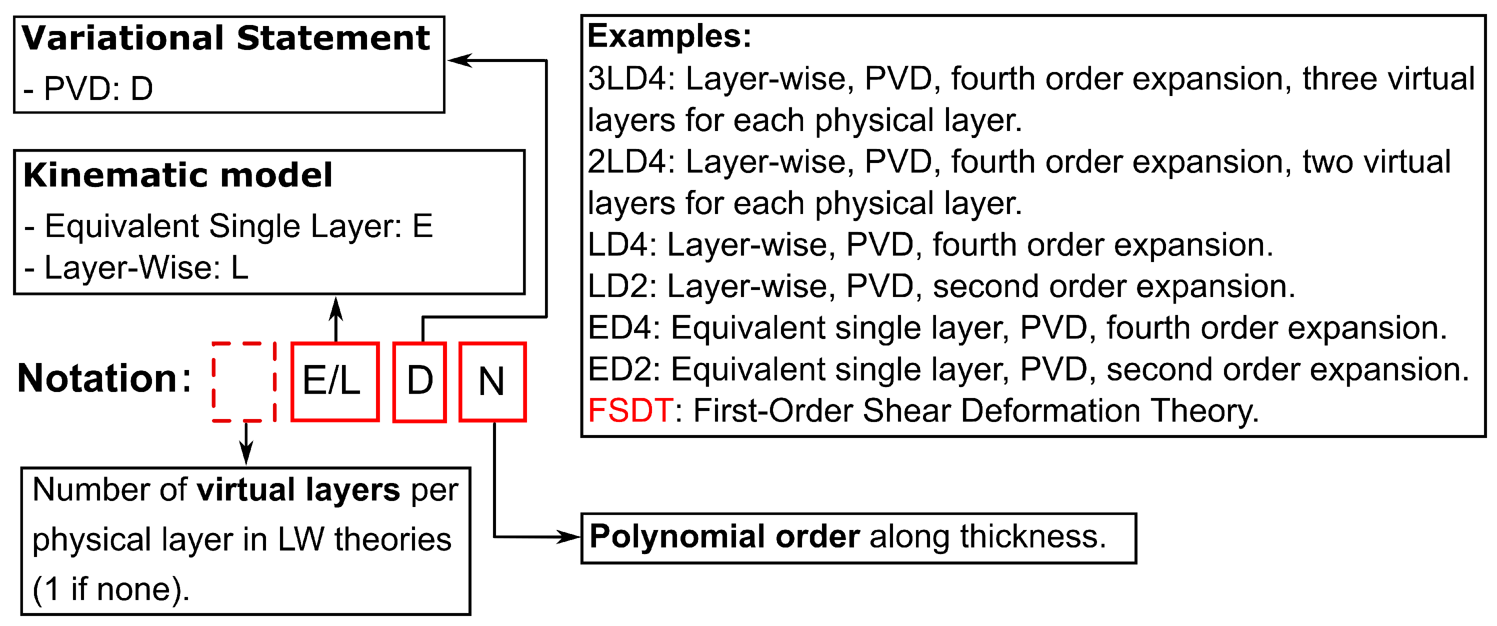
An acronym system is introduced in order to identify all the derived theories as shown in Figure 3.

The first letter refers to the approximation level that is used: ‘E’ corresponds to ESL models while ‘L’ corresponds to LW models. The second letter refers to the variational statement: ‘D’ stands for PVD. The last number refers to the expansion order used along the structure thickness. The first number, when present, refers to the number of virtual layers that have been used for an LW model to represent every single physical layer; if the number at the beginning of the acronym is not present, it is assumed that only one virtual layer has been used for each physical layer.

As an example of the used acronym system, in EDN models, the displacement field is expressed in the following form:

$$\begin{array}{ccc}{u}_{\alpha }\hfill & =\hfill & u_{\alpha 0}+u_{\alpha 1}z+u_{\alpha 2}{z}^2+\cdots +u_{\alpha N}{z}^N,\hfill \\ u_{\beta }\hfill & =\hfill & u_{\beta 0}+u_{\beta 1}z+u_{\beta 2}{z}^2+\cdots +u_{\beta N}{z}^N,\hfill \\ u_z\hfill & =\hfill & u_{z0}+u_{z1}z+u_{z2}{z}^2+\cdots +u_{zN}{z}^N.\hfill \end{array}$$

(31)

In a vectorial form:

$$\mathbf{u}=F_0{\mathbf{u}}_0+F_1{\mathbf{u}}_1+\cdots +F_N{\mathbf{u}}_N=F_{\tau }{\mathbf{u}}_{\tau },\tau =0,1,\dots ,N,$$

(32)

where $F_{\tau }=z^{\tau }$ and ${\mathbf{u}}_{\tau }={\mathbf{u}}_{\tau }\left(\alpha ,\beta \right)$. Also, the first-order shear deformation theory is indicated as FSDT and is obtained as a particular case of an ED1 solution. Specifically, FSDT is obtained through the penalization of the $u_{z1}$ term, and the material stiffness matrix, as classically performed, is reduced to account for a plane stress state and resolve thickness locking.

In LW theories, N refers to the approximation order used in every layer:

$${\mathbf{u}}^k=F_0{\mathbf{u}}_0^k+F_1{\mathbf{u}}_1^k+\cdots +F_N{\mathbf{u}}_N^k=F_{\tau }{\mathbf{u}}_{\tau }^k,\tau =0,1,\dots ,N,k=1,2,\dots ,N_l.$$

(33)

It can be observed that ESL theories can be considered as a particular case of LW ones. While, in the first case, the integration along the thickness is performed in order to represent composite properties through an equivalent single layer, for the second case, the integration is computed layer by layer. This allows one to represent the kinematic of each layer separately for LW models. Unless otherwise stated, LDN solutions are obtained with Lagrange polynomials with equally spaced nodes.

2.5. Locking Correction

The locking phenomenon is common for shells’ finite elements and it is well known in the literature. Its correction is performed through the mixed interpolation of tensorial components (MITC) method. This method is based on the idea of considering the interpolation of the strain components on specific points of the element domain, which are called “tying points”, and it is implemented by considering the strain tensor in the local coordinate system of each element, defined by $\xi$, $\eta$ and $\zeta$ axes. The location of the tying points depends on the strain component being interpolated and on the number of nodes of the element. In this work, nine-node elements using the MITC approach are used. They are named MITC9 shell elements. Three different patterns are used for the tying points in this case, as shown in Figure 4.

Classical Lagrange polynomials are used as interpolation functions and they are defined referring to the points of each interpolation scheme. These function are grouped into the following vectors:

$$\begin{array}{c}{\mathbf{N}}_{m1}=\left[N_{A1},N_{B1},N_{C1},N_{D1},N_{E1},N_{F1}\right],\hfill \\ {\mathbf{N}}_{m2}=\left[N_{A2},N_{B2},N_{C2},N_{D2},N_{E2},N_{F2}\right],\hfill \\ {\mathbf{N}}_{m3}=\left[N_P,N_Q,N_R,N_S\right].\hfill \end{array}$$

(34)

The strain components are interpolated in the following way:

$${ϵ}_p=\left[\begin{array}{c}{ϵ}_{\xi \xi }\hfill \\ {ϵ}_{\eta \eta }\hfill \\ {ϵ}_{\xi \eta }\hfill \end{array}\right]=\left[\begin{array}{ccc}{\mathbf{N}}_{m1}& 0& 0\\ 0& {\mathbf{N}}_{m2}& 0\\ 0& 0& {\mathbf{N}}_{m3}\end{array}\right]\left[\begin{array}{c}{ϵ}_{\xi {\xi }_{m1}}\hfill \\ {ϵ}_{\eta {\eta }_{m2}}\hfill \\ {ϵ}_{\xi {\eta }_{m3}}\hfill \end{array}\right]=\mathbf{N}\mathbf{1}\left[\begin{array}{c}{ϵ}_{\xi {\xi }_{m1}}\hfill \\ {ϵ}_{\eta {\eta }_{m2}}\hfill \\ {ϵ}_{\xi {\eta }_{m3}}\hfill \end{array}\right],$$

(35)

$${ϵ}_n=\left[\begin{array}{c}{ϵ}_{\xi z}\hfill \\ {ϵ}_{\eta z}\hfill \\ {ϵ}_{zz}\hfill \end{array}\right]=\left[\begin{array}{ccc}{\mathbf{N}}_{m1}& 0& 0\\ 0& {\mathbf{N}}_{m2}& 0\\ 0& 0& 1\end{array}\right]\left[\begin{array}{c}{ϵ}_{\xi z_{m1}}\hfill \\ {ϵ}_{\eta z_{m2}}\hfill \\ {ϵ}_{zz}\hfill \end{array}\right]=\mathbf{N}\mathbf{2}\left[\begin{array}{c}{ϵ}_{\xi z_{m1}}\hfill \\ {ϵ}_{\eta z_{m2}}\hfill \\ {ϵ}_{zz}\hfill \end{array}\right],$$

(36)

where the subscripts $m1$, $m2$ and $m3$ indicate that the quantities are calculated in the points (A1, B1, C1, D1, E1, F1), (A2, B2, C2, D2, E2, F2) and (P, Q, R, S), respectively.

2.6. FEM Matrices Expression

In the PVD case, the primary unknown field is the displacements field. Considering Equation (30), the displacements field can be written as follows:

$$\mathbf{u}=F_{\tau }{N}_i\left\{\begin{array}{c}{q}_{\alpha \tau i}\\ q_{\beta \tau i}\\ q_{z\tau i}\end{array}\right\}=F_{\tau }{N}_i{\mathbf{q}}_{\tau i}.$$

(37)

Through the substitution of Equations (25), (24), (16), (20) and (37), into Equation (23), the weak form of the PVD method can be obtained:

$$\begin{array}{cc}\hfill {\int }_{\mathrm{\Omega }}& \delta {\mathit{q}}_{\tau i}^T[{\left(\mathbf{N}{\mathbf{1}}_m{\mathbf{D}}_p\right)}^T\left(N_i\mathbf{I}\right){\tilde{\mathbf{Z}}}_{pp}^{\tau s}\left(\mathbf{N}{\mathbf{1}}_o{\mathbf{D}}_p\right)\left(N_j\mathbf{I}\right)+{\left(\mathbf{N}{\mathbf{1}}_m{\mathbf{D}}_p\right)}^T\left(N_i\mathbf{I}\right){\tilde{\mathbf{Z}}}_{pp}^{\tau s}\left(\mathbf{N}{\mathbf{1}}_o{\mathbf{A}}_p\right)\left(N_j\mathbf{I}\right)+\hfill \\ \hfill +& {\left(\mathbf{N}{\mathbf{1}}_m{\mathbf{D}}_p\right)}^T\left(N_i\mathbf{I}\right){\tilde{\mathbf{Z}}}_{pn}^{\tau s}\left(\mathbf{N}{\mathbf{2}}_o{\mathbf{D}}_{n\mathrm{\Omega }}\right)\left(N_j\mathbf{I}\right)+{\left(\mathbf{N}{\mathbf{1}}_m{\mathbf{D}}_p\right)}^T\left(N_i\mathbf{I}\right){\tilde{\mathbf{Z}}}_{pn}^{\tau s}\left(\mathbf{N}{\mathbf{2}}_o{\mathbf{A}}_n\right)\left(N_j\mathbf{I}\right)+\hfill \\ \hfill +& {\left(\mathbf{N}{\mathbf{1}}_m{\mathbf{D}}_p\right)}^T\left(N_i\mathbf{I}\right){\tilde{\mathbf{Z}}}_{pn}^{\tau s{,}_z}\mathbf{N}{\mathbf{2}}_o\left(N_j\mathbf{I}\right)+{\left(\mathbf{N}{\mathbf{1}}_m{\mathbf{A}}_p\right)}^T\left(N_i\mathbf{I}\right){\tilde{\mathbf{Z}}}_{pp}^{\tau s}\left(\mathbf{N}{\mathbf{1}}_o{\mathbf{D}}_p\right)\left(N_j\mathbf{I}\right)+\hfill \\ \hfill +& {\left(\mathbf{N}{\mathbf{1}}_m{\mathbf{A}}_p\right)}^T\left(N_i\mathbf{I}\right){\tilde{\mathbf{Z}}}_{pp}^{\tau s}\left(\mathbf{N}{\mathbf{1}}_o{\mathbf{A}}_p\right)\left(N_j\mathbf{I}\right)+{\left(\mathbf{N}{\mathbf{1}}_m{\mathbf{A}}_p\right)}^T\left(N_i\mathbf{I}\right){\tilde{\mathbf{Z}}}_{pn}^{\tau s}\left(\mathbf{N}{\mathbf{2}}_o{\mathbf{D}}_{n\mathrm{\Omega }}\right)\left(N_j\mathbf{I}\right)+\hfill \\ \hfill +& {\left(\mathbf{N}{\mathbf{1}}_m{\mathbf{A}}_p\right)}^T\left(N_i\mathbf{I}\right){\tilde{\mathbf{Z}}}_{pn}^{\tau s}\left(\mathbf{N}{\mathbf{2}}_o{\mathbf{A}}_n\right)\left(N_j\mathbf{I}\right)+{\left(\mathbf{N}{\mathbf{1}}_m{\mathbf{A}}_p\right)}^T\left(N_i\mathbf{I}\right){\tilde{\mathbf{Z}}}_{pn}^{\tau s{,}_z}\mathbf{N}{\mathbf{2}}_o\left(N_j\mathbf{I}\right)+\hfill \\ \hfill +& {\left(\mathbf{N}{\mathbf{2}}_m{\mathbf{D}}_{n\mathrm{\Omega }}\right)}^T\left(N_i\mathbf{I}\right){\tilde{\mathbf{Z}}}_{np}^{\tau s}\left(\mathbf{N}{\mathbf{1}}_o{\mathbf{D}}_p\right)\left(N_j\mathbf{I}\right)+{\left(\mathbf{N}{\mathbf{2}}_m{\mathbf{D}}_{n\mathrm{\Omega }}\right)}^T\left(N_i\mathbf{I}\right){\tilde{\mathbf{Z}}}_{np}^{\tau s}\left(\mathbf{N}{\mathbf{1}}_o{\mathbf{A}}_p\right)\left(N_j\mathbf{I}\right)+\hfill \\ \hfill +& {\left(\mathbf{N}{\mathbf{2}}_m{\mathbf{D}}_{n\mathrm{\Omega }}\right)}^T\left(N_i\mathbf{I}\right){\tilde{\mathbf{Z}}}_{nn}^{\tau s}\left(\mathbf{N}{\mathbf{2}}_o{\mathbf{D}}_{n\mathrm{\Omega }}\right)\left(N_j\mathbf{I}\right)+{\left(\mathbf{N}{\mathbf{2}}_m{\mathbf{D}}_{n\mathrm{\Omega }}\right)}^T\left(N_i\mathbf{I}\right){\tilde{\mathbf{Z}}}_{nn}^{\tau s}\left(\mathbf{N}{\mathbf{2}}_o{\mathbf{A}}_n\right)\left(N_j\mathbf{I}\right)+\hfill \\ \hfill +& {\left(\mathbf{N}{\mathbf{2}}_m{\mathbf{D}}_{n\mathrm{\Omega }}\right)}^T\left(N_i\mathbf{I}\right){\tilde{\mathbf{Z}}}_{nn}^{\tau s{,}_z}\mathbf{N}{\mathbf{2}}_o\left(N_j\mathbf{I}\right)+{\left(\mathbf{N}{\mathbf{2}}_m{\mathbf{A}}_n\right)}^T\left(N_i\mathbf{I}\right){\tilde{\mathbf{Z}}}_{np}^{\tau s}\left(\mathbf{N}{\mathbf{1}}_o{\mathbf{D}}_p\right)\left(N_j\mathbf{I}\right)+\hfill \\ \hfill +& {\left(\mathbf{N}{\mathbf{2}}_m{\mathbf{A}}_n\right)}^T\left(N_i\mathbf{I}\right){\tilde{\mathbf{Z}}}_{np}^{\tau s}\left(\mathbf{N}{\mathbf{1}}_o{\mathbf{A}}_p\right)\left(N_j\mathbf{I}\right)+{\left(\mathbf{N}{\mathbf{2}}_m{\mathbf{A}}_n\right)}^T\left(N_i\mathbf{I}\right){\tilde{\mathbf{Z}}}_{nn}^{\tau s}\left(\mathbf{N}{\mathbf{2}}_o{\mathbf{D}}_{n\mathrm{\Omega }}\right)\left(N_j\mathbf{I}\right)+\hfill \\ \hfill +& {\left(\mathbf{N}{\mathbf{2}}_m{\mathbf{A}}_n\right)}^T\left(N_i\mathbf{I}\right){\tilde{\mathbf{Z}}}_{nn}^{\tau s}\left(\mathbf{N}{\mathbf{2}}_o{\mathbf{A}}_n\right)\left(N_j\mathbf{I}\right)+{\left(\mathbf{N}{\mathbf{2}}_m{\mathbf{A}}_n\right)}^T\left(N_i\mathbf{I}\right){\tilde{\mathbf{Z}}}_{nn}^{\tau s{,}_z}\mathbf{N}{\mathbf{2}}_o\left(N_j\mathbf{I}\right)+\hfill \\ \hfill +& \mathbf{N}{\mathbf{2}}_m\left(N_i\mathbf{I}\right){\tilde{\mathbf{Z}}}_{np}^{\tau {,}_{z}s}\left(\mathbf{N}{\mathbf{1}}_o{\mathbf{D}}_p\right)\left(N_j\mathbf{I}\right)+\mathbf{N}{\mathbf{2}}_m\left(N_i\mathbf{I}\right){\tilde{\mathbf{Z}}}_{np}^{\tau {,}_{z}s}\left(\mathbf{N}{\mathbf{1}}_o{\mathbf{A}}_p\right)\left(N_j\mathbf{I}\right)+\hfill \\ \hfill +& \mathbf{N}{\mathbf{2}}_m\left(N_i\mathbf{I}\right){\tilde{\mathbf{Z}}}_{nn}^{\tau {,}_{z}s}\left(\mathbf{N}{\mathbf{2}}_o{\mathbf{D}}_{n\mathrm{\Omega }}\right)\left(N_j\mathbf{I}\right)+\mathbf{N}{\mathbf{2}}_m\left(N_i\mathbf{I}\right){\tilde{\mathbf{Z}}}_{nn}^{\tau {,}_{z}s}\left(\mathbf{N}{\mathbf{2}}_o{\mathbf{A}}_n\right)\left(N_j\mathbf{I}\right)+\hfill \\ \hfill +& \mathbf{N}{\mathbf{2}}_m\left(N_i\mathbf{I}\right){\tilde{\mathbf{Z}}}_{nn}^{\tau {,}_{z}s{,}_z}\mathbf{N}{\mathbf{2}}_o\left(N_j\mathbf{I}\right)]{\mathit{q}}_{sj}d\mathrm{\Omega }=-{\int }_{\mathrm{\Omega }}\delta {\mathit{q}}_{\tau i}^T\left(N_i\mathbf{I}\right)\rho E_{\tau s}\left(N_j\mathbf{I}\right){\ddot{\mathit{q}}}_{sj}d\mathrm{\Omega },\hfill \end{array}$$

(38)

where

$$({\tilde{\mathbf{Z}}}_{wr}^{\tau s},{\tilde{\mathbf{Z}}}_{wr}^{\tau {,}_{z}s},{\tilde{\mathbf{Z}}}_{wr}^{\tau s{,}_z},{\tilde{\mathbf{Z}}}_{wr}^{\tau {,}_{z}s{,}_z})=({\tilde{\mathbf{C}}}_{wr}{E}_{\tau s},{\tilde{\mathbf{C}}}_{wr}{E}_{\tau {,}_{z}s},{\tilde{\mathbf{C}}}_{wr}{E}_{\tau s{,}_z},{\tilde{\mathbf{C}}}_{wr}{E}_{\tau {,}_{z}s{,}_z}):w,r=p,n,$$

(39)

$$(E_{\tau s},E_{\tau {,}_{z}s},E_{\tau s{,}_z},E_{\tau {,}_{z}s{,}_z})={\int }_h(F_{\tau }{F}_s,F_{\tau {,}_z}{F}_s,F_{\tau }{F}_{s{,}_z},F_{\tau {,}_z}{F}_{s{,}_z})dz.$$

(40)

Indices $\tau$, i and m refer to virtual variations, while s, j and o refer to real quantities. In a compact vectorial form, Equation (38) reads as follows:

$$\delta {\mathit{q}}_{\tau i}^T{\mathbf{K}}^{\tau sij}{\mathit{q}}_{sj}=-\delta {\mathit{q}}_{\tau i}^T{\mathbf{M}}^{\tau sij}{\ddot{\mathit{q}}}_{sj},$$

(41)

where ${\mathbf{K}}^{\tau sij}$ and ${\mathbf{M}}^{\tau sij}$ are the $3\times 3$ fundamental nuclei (FN) of the stiffness and mass matrices, respectively. The components of the FN are reported in Appendix A. Through the loops on the indices $\tau$, s, i and j, it is possible to build the stiffness and mass matrices of the whole shell. The mid-surface integrals are computed through Gauss quadrature with a $3\times 3$ grid of points to integrate all the terms of the FN. The algorithm is implemented in Python and the eigenvalue problem described by Equation (38) is solved using the scipy.linalg.eigh function from the SciPy library. This function utilizes LAPACK drivers to solve standard or generalized eigenvalue problems for complex Hermitian or real symmetric matrices.

3. Numerical Results and Discussion

Three benchmark problems are considered in this section: a monolayer cylindrical shell, a monolayer cylinder and a bi-layer spherical segment. Parametric studies are performed considering different values of thickness as the other geometrical parameter constant. Material properties are represented in

Table 1. Material properties.

Case	${\mathit{E}}_{\mathit{L}}$ [GPa]	${\mathit{E}}_{\mathit{T}}$ [GPa]	${\mathit{G}}_{\mathit{L}\mathit{T}}$ [GPa]	${\mathit{G}}_{\mathit{T}\mathit{T}}$ [GPa]	${\mathit{\nu }}_{\mathit{L}\mathit{T}}$, ${\mathit{\nu }}_{\mathit{T}\mathit{T}}$
1, 2, 3	50	10	5	5	$0.25$

. The subscript “L” refers to the longitudinal direction of the fibers, while subscript “T” refers to the transverse fibers’ direction.

Reference solutions are represented by Abaqus 3D models, where quadratic solid elements with reduced integration and three degrees of freedom per node (C3D20R) are used. In Abaqus 3D solutions, the orientation is assumed to remain constant within each element and corresponds to the fiber angle at the centroid of the respective element. Consequently, a refined mesh is required to achieve accurate results. The material orientation is assigned on an element-by-element basis using Python scripting (version 3.9.10) in Abaqus 2018. A frequency step is defined to compute the first fifteen eigenvalues, with the default Lanczos eigensolver employed. The analysis utilizes three CPUs for parallel processing to enhance computational efficiency. For CUF solutions, nine-node square elements are used (QUAD9). The software Gmsh is used to generate the mesh and represent the modal shapes during post-processing. For each case study, an initial convergence analysis is performed to determine the suitable mesh for both CUF and Abaqus solutions. Percentage errors are evaluated as follows:

$${\delta }_{\mathrm{err}\%}={\displaystyle \frac{|{\varphi }_{i,\mathrm{CUF}}-{\varphi }_{i,\mathrm{Abaqus}3\mathrm{D}}|}{|{\varphi }_{i,\mathrm{Abaqus}3\mathrm{D}}|}}·100,$$

(42)

where ${\varphi }_i$ is the modal frequency corresponding to the i-th mode. The effective mass percentage is used to obtain a deeper physical understanding of the modal behavior of the analyzed structures. Indeed, this value represents the amount of the total mass that participates in a given mode of vibration. This parameter is determined through the Abaqus 3D model and can be calculated as follows:

$$m_{\mathrm{err}\%,i}={\displaystyle \frac{m_{\mathrm{eff},i}}{m_{\mathrm{tot}}}}·100,i=X,Y,Z.$$

(43)

Here, $m_{\mathrm{eff},i}$ represents the effective mass in one of the directions defined by the axes of the global Cartesian reference system, while $m_{\mathrm{tot}}$ denotes the total mass of the shell. To ensure that the number of considered modes is sufficient for describing the modal behavior of the structure, the sum of the effective masses along each direction should closely approximate the total mass of the system. However, since this is not the primary objective of this work, only the first six natural frequencies are considered for all the studied cases. Further details regarding the computation of effective masses are omitted for the sake of brevity but can be found in the Abaqus Theory Manual [48].

3.1. Monolayer Cylindrical Shell

The first case corresponds to a monolayer portion of the cylindrical surface with the following dimensions: $R_{\alpha }=1$ m, $l_{\alpha }=R_{\alpha }\pi /4$ m, $l_{\beta }=2l_{\alpha }$. The reference systems that have been used to describe the problem are represented in Figure 5.

The radius vector is defined as

$$\mathbf{r}=\left\{\begin{array}{c}{R}_{\alpha }sin\left(\gamma \right)\\ Y\\ R_{\alpha }cos\left(\gamma \right)\end{array}\right\}.$$

(44)

Considering $\alpha =R_{\alpha }\gamma$ and $\beta =Y$, the coefficients of the first quadratic form are defined as follows:

$$A=1,B=1,$$

(45)

and, as a consequence,

$$H_{\alpha }=\left(1+{\displaystyle \frac{z}{R_{\alpha }}}\right),H_{\beta }=1.$$

(46)

It is assumed that the fibers’ angle is a function of $y^{\prime }$. For this problem, axes $x^{\prime }$ and $y^{\prime }$ of the local reference system of the fibers’ path are coincident with axes $\alpha$ and $\beta$ of the curvilinear reference system of the shell. Therefore, the characteristic length of Equation (22) is set to $d=l_{\beta }$. The angle variational law is expressed as $90<0,90>$, and it is taken from Viglietti et al. [49], where it is applied on a rectangular plate for vibration analyses. The fiber orientation within the shell is illustrated in Figure 6, where the axis labeled “1” represents the tangent direction of a fiber at a specific point.

The shell is fully clamped with density $\rho =1540$ kg/m³. The Abaqus reference solution contains 12 elements along the thickness, while 40 and 80 elements are used along $\alpha$ and $\beta$, respectively. For the CUF results, a $10\times 20$ mesh is considered.

Table 2. Number of degrees of freedom, case 1.

	DOF
Abaqus 3D	503,355
2LD4	23,247
2LD2	12,915
ED6	18,081
ED4	12,915
ED2	7749
FSDT	5166

shows the number of degrees of freedom (DoF) for the considered solutions. FSDT shows the smallest number of DoF since it is obtained through a manipulation of the ED1 model.

It is possible to observe that the Abaqus reference solution is characterized by a number of DoF which is at least one order of magnitude bigger than CUF solutions. This shows that the developed models guarantee a reduction in the computational cost in terms of DoF.

Table 3. Natural frequencies (${10}^2·$rad/s), $l_{\alpha }/h=100$, case 1.

	1	2	3	4	5	6
Abaqus 3D	10.843	13.862	16.123	18.316	20.670	21.881
2LD4	10.858	13.911	16.145	18.374	20.701	21.946
2LD2	10.859	13.912	16.145	18.375	20.702	21.947
ED6	10.858	13.911	16.145	18.374	20.701	21.946
ED4	10.858	13.911	16.145	18.374	20.701	21.946
ED2	10.861	13.918	16.149	18.386	20.708	21.963
FSDT	10.852	13.893	16.142	18.366	20.700	21.944

shows the first six modal frequencies for different theories in the case $l_{\alpha }/h=100$.

For this case, all the theories show a comparable level of accuracy. This happens because a thin shell is considered and a linear law is sufficient for approximating the displacements along the thickness, as shown by the FSDT theory, which is characterized by a maximum error of $0.29\%$ for the sixth frequency. When the aspect ratio is reduced, the thickness of the shell is increased and the differences among the various theories become more evident.

Table 4. Natural frequencies (${10}^2·$rad/s), $l_{\alpha }/h=10$, case 1.

	1	2	3	4	5	6
Abaqus 3D	40.262	52.831	63.309	65.599	77.539	81.103
2LD4	40.283	52.854	63.353	65.669	77.597	81.175
2LD2	40.309	52.900	63.429	65.787	77.723	81.371
ED6	40.283	52.854	63.353	65.669	77.597	81.176
ED4	40.286	52.858	63.362	65.685	77.613	81.202
ED2	40.596	53.404	64.197	66.943	78.937	83.210
FSDT	40.551	53.374	64.144	66.830	78.881	83.132

shows the first six modal frequencies considering $l_{\alpha }/h=10$.

It is possible to observe that, in this case, the FSDT model shows the worst approximation and the percentage error on the sixth mode grows to $2.50\%$. This error can be reduced to $0.09\%$ with 2LD4 and ED6 models. Moreover, the error of FSDT grows when higher frequencies are considered. This is less evident for higher-order theories, which are able to better predict the reference solution even for higher frequencies. The first and the second modes show two and three semi-waves along the $\alpha$-axis, respectively, and one semi-wave along $\beta$. The third mode exhibits two semi-waves along both $\alpha$ and $\beta$ directions. The fourth mode shows three semi-waves along $\alpha$ and two semi-waves along $\beta$. The fifth mode presents two semi-waves along $\alpha$ and three semi-waves along $\beta$. Finally, the sixth mode shows three semi-waves along $\alpha$ and $\beta$.

Table 5. Effective mass percentage $m_{\mathrm{err}\%,i}$, $l_{\alpha }/h=10$, case 1.

	1	2	3	4	5	6
$m_{\mathrm{err}\%,X}$	4.7	1.0	– *	7.8	0.3	1.7
$m_{\mathrm{err}\%,Y}$	– *	– *	– *	– *	– *	0.2
$m_{\mathrm{err}\%,Z}$	34.8	3.9	11.7	0.3	0.2	– *

* Values below ${10}^{-1}$ are considered as negligible and marked with “–”.

shows the percentage of effective masses for the first six modal frequencies considering $l_{\alpha }/h=10$.

As evident from the table, the first mode is the most significant among the presented modes, as it involves the highest effective mass percentage along the Z-axis. This behavior can be attributed to the boundary conditions of the analyzed shell: since the structure is clamped and has a limited curvature, the first mode typically corresponds to a predominant displacement along the axis perpendicular to the boundaries, as observed in this case. The displacement of the structure mass along the Z-axis is most prominent in the first three modes. In contrast, the fourth mode exhibits a predominant displacement along the X-axis, while the fifth mode does not demonstrate a principal displacement direction compared to the previous ones. The sixth mode shows a slightly higher effective mass percentage along the X-axis. In this case, the first, second and third modes show one, two and three semi-waves along $\beta$, respectively, and one semi-wave along $\alpha$. The number of semi-waves increases in both directions for higher modes.

Table 6. Natural frequencies (${10}^2·$rad/s), $l_{\alpha }/h=5$, case 1.

	1	2	3	4	5	6
Abaqus 3D	55.388	70.438	86.799	93.100	103.030	108.270
2LD4	55.402	70.459	86.828	93.155	103.049	108.317
2LD2	55.545	70.674	87.128	93.550	103.195	108.755
ED6	55.403	70.460	86.829	93.157	103.050	108.318
ED4	55.425	70.494	86.881	93.239	103.080	108.401
ED2	56.714	72.344	89.328	95.873	104.149	111.735
FSDT	56.610	72.277	89.261	95.692	103.999	111.657

shows the first six modal frequencies for $l_{\alpha }/h=5$. The FSDT maximum error increases to $3.13\%$ for the sixth mode and can be reduced to $0.4\%$ via a 2LD4 model. In this case, the first three modes and the fifth one are similar to the $l_{\alpha }/h=10$ shell. The fourth mode shows two semi-waves along $\alpha$ and one semi-wave along $\beta$. The sixth mode displays four semi-waves along $\beta$ and one along $\alpha$.

3.2. Monolayer Cylinder

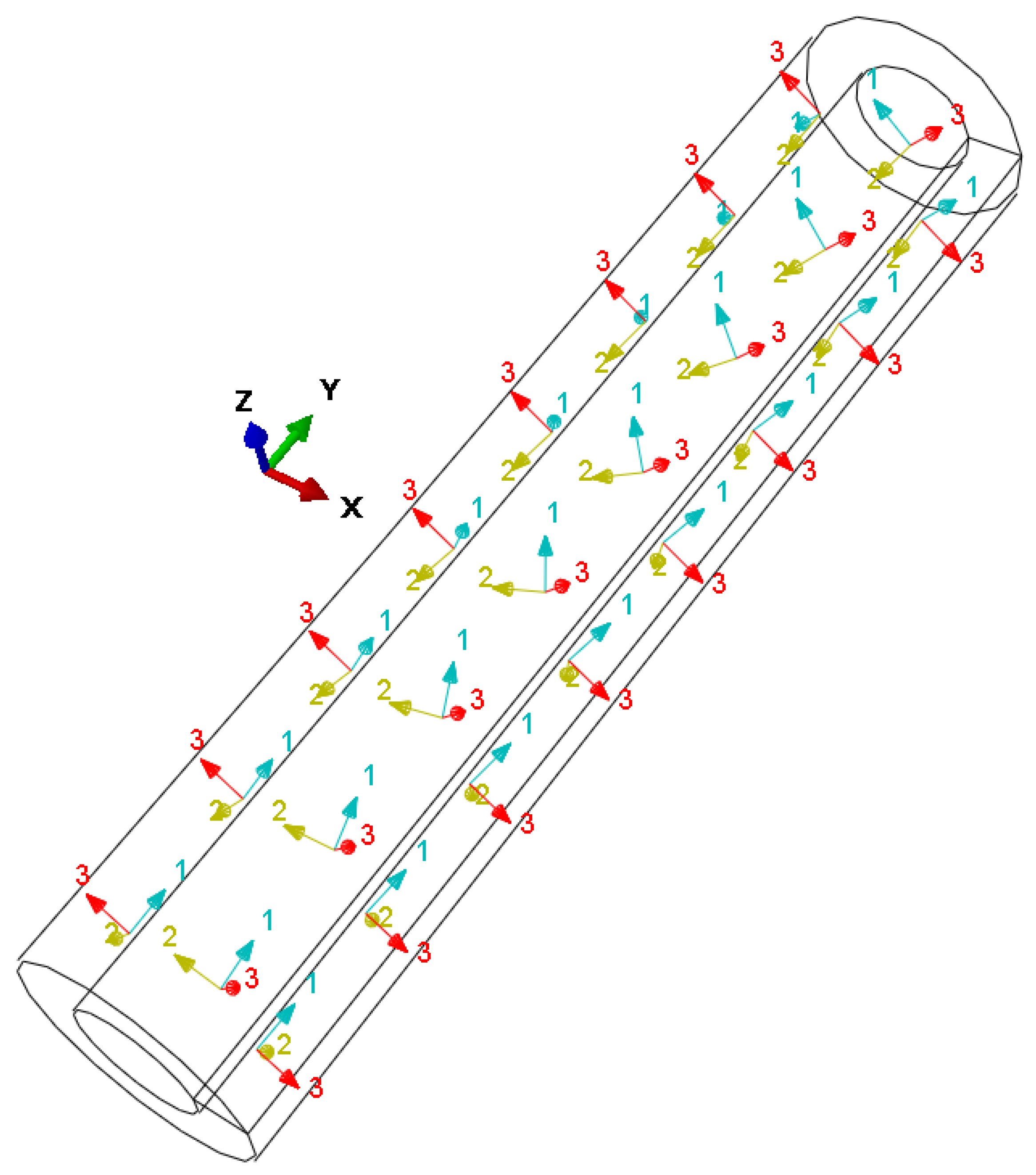
The second case corresponds to a cylindrical surface with a single layer. The following dimensions are considered: $R_{\alpha }=1$ m, $l_{\alpha }=2R_{\alpha }\pi$, $l_{\beta }=2l_{\alpha }$. The same reference systems, radius vector and coefficients of the first quadratic form of the middle surface as for the previous case are used. Also, the same $90<0,90>$ variation law of the previous case is considered for the fibers’ angle. The fiber orientation within the cylinder is illustrated in Figure 7, where the axis labeled “1” represents the tangent direction of a fiber at a specific point.

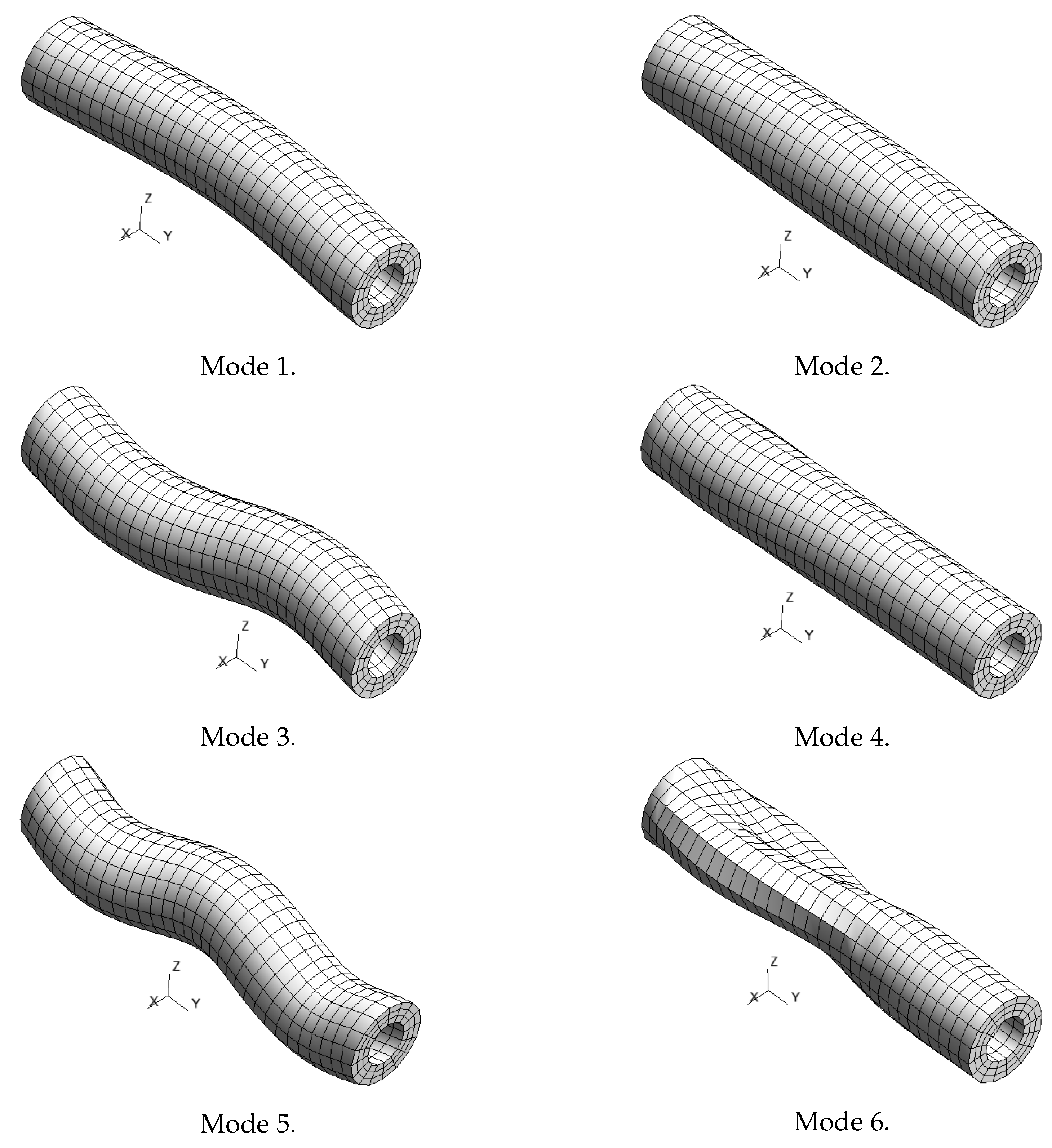
For this problem, axes $x^{\prime }$ and $y^{\prime }$ of the local reference system of the fibers’ path are coincident with axes $\alpha$ and $\beta$ of the curvilinear reference system of the shell. In this case, $l_{\beta }$ is considered as the characteristic length in Equation (22) ($d=l_{\beta }$). As for the previous case, the Abaqus reference solution contains 40 elements along $\alpha$, 80 elements along $\beta$ and 12 elements along the thickness. For CUF results, 8 elements are used in the $\alpha$ direction, while 16 elements are used along $\beta$. The cylinder is clamped at its ends ($\beta =0$ and $\beta =l_{\beta }$). Since the structure is axisymmetric, frequencies with a multiplicity higher than one are expected. The corresponding modal shapes are the same, apart from a rotation around the main axis of the cylinder. For the sake of brevity, repeated modes are presented only once. The first six modal frequencies are shown in

Table 7. Natural frequencies ($10·$rad/s), $l_{\alpha }/h=100$, case 2.

	1	2	3	4	5	6
Abaqus 3D	21.656	24.166	32.512	43.473	46.874	48.037
2LD4	21.737	24.172	32.531	45.266	46.876	47.853
2LD2	21.738	24.172	32.532	45.269	46.876	47.855
ED6	21.737	24.172	32.531	45.266	46.876	47.853
ED4	21.737	24.172	32.531	45.266	46.876	47.853
ED2	21.750	24.173	32.550	45.301	46.876	47.873
FSDT	21.760	24.155	32.590	45.277	46.874	47.928

in the case of $l_{\alpha }/h=100$.

In this case, the best approximation is given by 2LD4 and ED6 models, which both show a maximum error of $4.12\%$ for the fourth modal frequency. Since a thin shell is considered, transverse stresses do not play an important role. Therefore, classical and low-order theories provide good results. The first frequency corresponds to a radial mode with two semi-waves in the circumferential direction and one semi-wave in the longitudinal direction. The second mode exhibits bending with one semi-wave along the cylinder axis. The third mode is a radial mode characterized by two semi-waves in the circumferential direction and two longitudinal semi-waves. The fourth mode involves radial displacements with three circumferential semi-waves and one semi-wave along the cylinder axis. The fifth mode represents a radial mode with no semi-waves in the circumferential direction and one semi-wave in the longitudinal direction. Finally, the sixth mode features two semi-waves in the circumferential direction and three semi-waves in the longitudinal direction.

Table 8. Natural frequencies ($10·$rad/s), $l_{\alpha }/h=10$, case 2.

	1	2	3	4	5	6
Abaqus 3D	26.336	47.354	57.253	88.047	94.851	103.540
2LD4	26.338	47.364	57.258	88.065	94.879	103.581
2LD2	26.346	47.365	57.284	88.067	94.934	103.585
ED6	26.338	47.364	57.258	88.065	94.879	103.581
ED4	26.340	47.364	57.263	88.066	94.889	103.581
ED2	26.397	47.374	57.473	88.075	95.344	103.621
FSDT	26.405	47.256	57.537	87.897	95.515	103.286

shows the first six modal frequencies for $l_{\alpha }/h=10$.

The best approximation is given by 2LD4 and ED6 models, which show a maximum error of $0.04\%$ for the sixth frequency. The modal shapes obtained through the ED4 model for $l_{\alpha }/h=10$ are shown in Figure 8. These shapes match the ones obtained in Abaqus, which are not reported here for the sake of brevity. Mode one, three and five are bending modes. Modes two and four exhibit both translation along the Y-axis and rotation about the same axis. Finally, in the sixth mode, radial and longitudinal displacements can be observed. The deformation associated with the sixth mode is concentrated near the bottom of the cylinder, close to $y=0$. This behavior can be explained by considering the fiber orientation: at the bottom, the fibers are aligned axially, whereas at the top, they are oriented circumferentially. As a result, the structure exhibits greater stiffness in the radial direction at $y=l_{\beta }$.

Table 9. Effective mass percentage $m_{\mathrm{err}\%,i}$, $l_{\alpha }/h=10$, case 2.

	1	2	3	4	5	6
$m_{\mathrm{err}\%,X}$	0.6	– *	2.7	– *	1.8	– *
$m_{\mathrm{err}\%,Y}$	– *	1.7	– *	59.4	– *	9.7
$m_{\mathrm{err}\%,Z}$	72.1	– *	– *	– *	9.2	– *

* Values below ${10}^{-1}$ are considered as negligible and marked with “–”.

shows the percentage of effective masses for the first six modal frequencies considering $l_{\alpha }/h=10$.

In this case, the predominant modes are the first and the fourth. The first mode involves significant displacement of the mass along the Z-axis. The fourth mode, as previously discussed, couples longitudinal displacement along the Y-axis with rotation about the same axis. Nevertheless, the table shows that the majority of the mass moves in the Y direction, indicating that the fourth mode is primarily a longitudinal mode. The same considerations can be applied to the sixth mode.

Table 10. Natural frequencies ($10·$rad/s), $l_{\alpha }/h=5$, case 2.

	1	2	3	4	5	6
Abaqus 3D	29.694	47.943	64.012	88.485	105.250	106.100
2LD4	29.697	47.958	64.017	88.495	105.278	106.165
2LD2	29.728	47.964	64.109	88.504	105.447	106.200
ED6	29.697	47.958	64.017	88.495	105.278	106.165
ED4	29.705	47.959	64.041	88.497	105.323	106.171
ED2	29.874	47.994	64.540	88.528	106.222	106.339
FSDT	29.972	47.984	64.819	88.273	106.695	106.618

shows the first six modal frequencies for $l_{\alpha }/h=5$. In this case, classical and lower-order theories are not sufficient for matching the modal frequencies of the reference solution because a thick shell is considered. For example, the FSDT shows the inversion of the fifth and sixth vibration modes due to its limitations in capturing the complex couplings inherent to these modes. Specifically, the fifth mode exhibits torsional–radial coupling, while the sixth mode involves a complex interaction between torsional and bending effects. Accurately modeling these phenomena requires the inclusion of higher-order deformation effects, which are accounted for in more advanced theories, enabling more precise and reliable predictions. It is also possible to notice that the difference between 2LD4 and ED6 theories is not evident because a monolayer structure is considered. Indeed, both these theories show the best approximation, which is characterized by a maximum error of $0.06\%$ for the sixth natural frequency. The first five modes of this case are similar to the ones of the $l_{\alpha }/h=10$ cylinder. The sixth mode shows radial displacements with zero semi-waves along $\alpha$ and two semi-waves along $\beta$.

3.3. Bi-Layer Spherical Segment

The last case corresponds to a spherical segment with two layers of equal thickness. This kind of surface is obtained by cutting a sphere with two parallel planes, with the first one passing by the sphere center. The geometry and reference systems of this case are shown in Figure 9. The following dimensions are considered: $R=R_{\alpha }=R_{\beta }=1$ m, $l_{\alpha }=R\pi /6$, $l_{\beta }=2R\pi$.

The radius vector is defined as

$$\mathbf{r}=\left\{\begin{array}{c}Rsin\left(\gamma \right)\\ Rcos\left(\gamma \right)sin\left(\theta \right)\\ Rcos\left(\gamma \right)cos\left(\theta \right)\end{array}\right\}.$$

(47)

Considering $\alpha =R\gamma$ and $\beta =R\theta$, the coefficients of the first quadratic form are defined as follows:

$$A=1,B=cos\left(\gamma \right).$$

(48)

As a consequence,

$$H_{\alpha }=\left(1+{\displaystyle \frac{z}{R}}\right),H_{\beta }=cos\left(\gamma \right)\left(1+{\displaystyle \frac{z}{R}}\right).$$

(49)

The angle variation of the fibers is such that continuity along the circumferential direction is ensured. It is assumed that the fibers’ angle is a function of $y^{\prime }$. Axes $x^{\prime }$ and $y^{\prime }$ of the local fibers’ reference system are parallel to $\alpha$ and $\beta$ and their origin $o^{\prime }$ is placed in correspondence of $\alpha =l_{\alpha }/2$ and $\beta =l_{\beta }/2$. Therefore, the characteristic length in Equation (22) is $d=l_{\beta }/2$. The stacking sequence can be expressed as $\left[90<0,-45>/90<0,45>\right]$. The fiber orientation within the sphere is illustrated in Figure 10, where the axis labeled “1” represents the tangent direction of a fiber at a specific point.

The Abaqus reference solution uses 18 elements along $\alpha$, 216 elements along $\beta$ and 12 elements along thickness. CUF solutions use three elements in the $\alpha$ direction and 36 elements in the $\beta$ direction. The spherical segment is clamped at the lower edge ($\alpha =0$), while the top edge is free ($\alpha =l_{\alpha }$). As already explained for the previous case, only the first frequency of each couple is presented in the following tables. The first six modal frequencies for $l_{\alpha }/h=100$ are presented in

Table 11. Natural frequencies ($10·$rad/s), $l_{\alpha }/h=100$, case 3.

	1	2	3	4	5	6
Abaqus 3D	51.095	57.514	59.244	73.896	85.980	91.735
LD4	51.666	57.842	60.297	75.704	86.271	94.557
LD2	51.667	57.843	60.298	75.707	86.272	94.561
ED6	51.666	57.843	60.297	75.705	86.272	94.557
ED4	51.666	57.843	60.297	75.705	86.272	94.558
ED2	51.674	57.849	60.309	75.722	86.278	94.582
FSDT	51.606	57.714	60.280	75.711	86.084	94.573

.

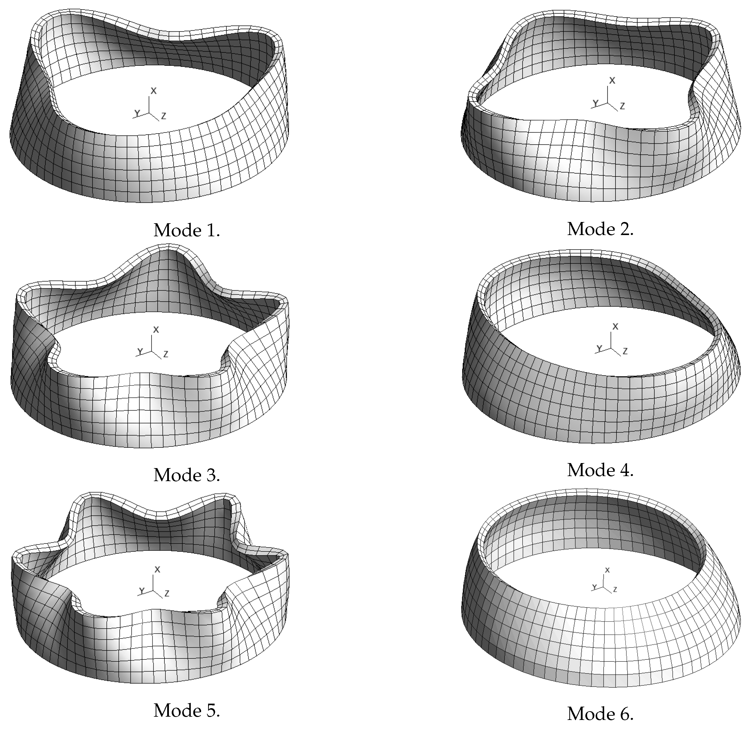
It is possible to observe that the theories show a good approximation of the reference results. In this case, all the modes show radial displacements along the $\beta$-axis. The first three modes show six, five and seven semi-waves, respectively. The fourth, fifth and sixth modes show eight, four and nine semi-waves, respectively. The percentage error of FSDT is $3.09\%$ for the sixth mode. For $l_{\alpha }/h=10$, the first six modal frequencies are displayed in

Table 12. Natural frequencies (${10}^2·$rad/s), $l_{\alpha }/h=10$, case 3.

	1	2	3	4	5	6
Abaqus 3D	18.724	19.391	24.738	25.494	32.710	35.354
LD4	18.789	19.489	24.917	25.555	32.978	35.473
LD2	18.795	19.501	24.937	25.558	33.009	35.475
ED6	18.789	19.489	24.918	25.555	32.979	35.475
ED4	18.790	19.491	24.921	25.557	32.984	35.480
ED2	18.836	19.562	25.046	25.595	33.182	35.541
FSDT	18.808	19.554	25.056	25.573	33.213	35.533

.

As previously noted, classical theories, and low-order theories in general, provide less accurate approximations of natural frequencies, particularly in cases with a low side-to-thickness ratio. Conversely, layer-wise theories offer the best approximation and align more closely with the Abaqus solution for higher frequencies. The modal shapes obtained through the ED4 model for $l_{\alpha }/h=10$ are shown in Figure 11. These shapes correspond to those obtained in Abaqus, which are not included here for the sake of brevity.

Table 13. Effective mass percentage $m_{\mathrm{err}\%,i}$, $l_{\alpha }/h=10$, case 3.

	1	2	3	4	5	6
$m_{\mathrm{err}\%,X}$	– *	– *	– *	– *	– *	0.3
$m_{\mathrm{err}\%,Y}$	0.1	– *	– *	– *	– *	0.2
$m_{\mathrm{err}\%,Z}$	– *	– *	– *	– *	– *	43.4

* Values below ${10}^{-1}$ are considered as negligible and marked with “–”.

shows the percentage of effective masses for the first six modal frequencies, considering $l_{\alpha }/h=10$.

In this case, the predominant mode is the sixth, which exhibits significant displacement of the structural mass along the Z-axis.

Table 14. Natural frequencies (${10}^2·$rad/s), $l_{\alpha }/h=5$, case 3.

	1	2	3	4	5	6
Abaqus 3D	25.989	28.627	32.082	36.316	42.619	51.291
LD4	26.068	28.699	32.207	36.407	42.808	51.430
LD2	26.097	28.721	32.267	36.417	42.905	51.440
ED6	26.068	28.701	32.208	36.414	42.811	51.440
ED4	26.074	28.709	32.217	36.430	42.824	51.459
ED2	26.271	28.853	32.597	36.575	43.442	51.645
FSDT	26.261	28.862	32.631	36.572	43.524	51.620

provides the first six modal frequencies for $l_{\alpha }/h=5$.

Since a thick shell is considered, the effect of transverse stresses is not negligible, which causes the classical and lower-order theories to be less inaccurate. This can be observed for FSDT, which has an error as high as $2.12\%$ for the fifth mode. This error can be reduced to $0.45\%$ and $0.44\%$ considering ED6 and LD4, respectively. In this case, the difference between ESL and LW models is more evident, since a multilayer shell is considered. Indeed, the possibility of obtaining a layer-wise representation of the laminate allows one to better predict the displacement field of each layer and, as a consequence, have more accurate values of the natural frequencies. The first mode is similar in both the $l_{\alpha }/h=10$ and the current case. The second mode shows two semi-waves in the circumferential direction. The third mode exhibits four semi-waves along $\beta$. The fourth mode shows simple bending along the X-axis. The fifth mode displays five semi-waves along $\beta$. Finally, the sixth mode shows an extension of the structure on the Y-Z plane, which corresponds to a radial mode with zero circumferential semi-waves.

4. Conclusions

This paper presents a numerical methodology for the free vibration analysis of VAT shells. The proposed approach is based on the use of the CUF within an FE context, where the governing equations are derived through the PVD, considering displacements as primary variables. The main innovation is the adaptation of this framework to shell structures characterized by a mid-surface with non-constant first quadratic form coefficients. As can be observed in Equation (18), non-constant A and B coefficients generate new terms in the ${\mathbf{A}}_p$ matrix, which has a direct influence on geometric relations. This also implies more complex terms in the FN of the stiffness matrix, since the derivatives $A{,}_{\beta }$, $B{,}_{\alpha }$, $H_{\alpha {,}_{\beta }}$ and $H_{\beta {,}_{\alpha }}$ need to be integrated. Considering variable coefficients of the first quadratic form enables the study of more complex geometries, laying the foundation for further research on variable curvature shells. Moreover, the formulation of the FN components is also applicable to shells with varying curvature radii. Three different cases of analysis are presented, and the results obtained through various CUF theories are validated with Abaqus 3D reference solutions. The variation in the fibers’ angle is described through linear laws, but the presented formulation is general and can be adapted to more complex fiber distributions. ESL and LW approaches are both considered and their performance is compared to FSDT. The latter offers a good balance between accuracy and computational cost; however, it provides less accurate predictions of the behavior of thick shells. This is evident in the second analysis case, where FSDT demonstrates a significant loss of accuracy in predicting high-frequency modes when the side-to-thickness ratio is equal to five. On the other hand, ESL and LW theories yield the best match of the reference 3D solution, independently from the shell geometry or fiber variational law. Moreover, the differences between ESL and LW theories are more evident in cases where shells with multiple layers are considered. Indeed, for those cases, a layer-wise description of the shell kinematics allows one to obtain more accurate displacement fields and, as a consequence, modal frequencies. Considering the same expansion order N along the thickness, when multiple layers are taken into account, LW theories exhibit higher computational costs compared to ESL theories. Consequently, the choice between using LW and ESL models should be guided by a balance between accuracy and computational cost. In conclusion, the application of PVD within CUF has shown the possibility of modeling VAT shells for free vibration analyses within an FE context. One of the main drawbacks of the presented approach is the need to account for the mid-surface equation to accurately represent the shell geometry. Consequently, the analysis process depends on the analytical representation of the surface, increasing the complexity of its application to generic geometries. Additionally, the significant increase in DOF for LW models is not always justified, particularly for thin plates. In such cases, the FSDT model remains advantageous, offering a better balance between computational cost and result accuracy. However, the FSDT is incorporated into the presented formulation and can be utilized as a first-order ESL model. The potential of this approach is not limited to the shells presented in this work. Potential prospects foresee the use of this framework for studying more complex VAT shells, characterized by a non-constant curvature radius. Moreover, more complex variational statements, like the Reissner’s mixed variational theorem, can be developed into this framework. This would enable the inclusion of transverse stresses as primary variables, further enhancing the accuracy of the solution. Additionally, the proposed approach can be extended to multi-field analyses, as the coupling between thermal, mechanical and electrical fields is of significant interest in various modern engineering applications, including aircraft and spacecraft design, aeroelasticity, wind turbine blades, actuators and sensors. In these contexts, additional advantages can be achieved by the ability to study surfaces with variable curvature radii and generic mid-surface geometries.

References

1. Brasington, A.; Sacco, C.; Halbritter, J.; Wehbe, R.; Harik, R. Automated fiber placement: A review of history, current technologies, and future paths forward. Compos. Part C Open Access 2021, 6, 100182. [Google Scholar] [CrossRef]
2. Kim, C.; Potter, K.; Weaver, M. Continuous tow shearing for manufacturing variable angle tow composites. Compos. Part A Appl. Sci. Manuf. 2012, 43, 1347–1356. [Google Scholar] [CrossRef]
3. Zhuo, P.; Li, S.; Ashcroft, A.; Jones, I. Material extrusion additive manufacturing of continuous fibre reinforced polymer matrix composites: A review and outlook. Compos. Part B Eng. 2021, 224, 109143. [Google Scholar] [CrossRef]
4. Brooks, T.R.; Martins, J.R.; Kennedy, G.J. High-fidelity aerostructural optimization of tow-steered composite wings. J. Fluids Struct. 2019, 88, 122–147. [Google Scholar] [CrossRef]
5. Grenoble, R.W.; Nguyen, T.; McKenney, M.J.; Przekop, A.; Juarez, P.D.; Gregory, E.D.; Jegley, D.C. Fabrication of a composite tow-steered structure for air-launch vehicle applications. In Proceedings of the AIAA/ASCE/AHS/ASC Structures, Structural Dynamics, and Materials Conference, Kissimmee, FL, USA, 8–12 January 2018. [Google Scholar]
6. Love, A.E.H. XVI. The small free vibrations and deformation of a thin elastic shell. Philos. Trans. R. Soc. A 1888, 179, 491–546. [Google Scholar]
7. Donnell, L.H. Stability of Thin-Walled Tubes Under Torsion; NASA: Washington, DC, USA, 1933.
8. Flügge, W. Stresses in Shells; Springer Science & Business Media: Berlin/Heidelberg, Germany, 2013. [Google Scholar]
9. Lindberg, G.M.; Olson, M.D.; Cowper, G.R. New developments in the finite element analysis of shells. Q. Bull. Div. Mech. Eng. Natl. Aeronaut. Establ. 1969, 4, 1–38. [Google Scholar]
10. Clough, R.W.; Johnson, C.P. A finite element approximation for the analysis of thin shells. Int. J. Solids 1969, 4, 43–60. [Google Scholar] [CrossRef]
11. Bogner, F.K.; Fox, R.L.; Schmit, L.A. A cylindrical shell discrete element. AIAA J. 1967, 5, 745–750. [Google Scholar] [CrossRef]
12. Maksymyuk, V.A. Locking phenomenon in computational methods of the shell theory. Int. J. Appl. Mech. 2020, 56, 347–350. [Google Scholar] [CrossRef]
13. Bathe, K.-J.; Dvorkin, E.N. A formulation of general shell elements—The use of mixed interpolation of tensorial components. Int. J. Numer. Methods Eng. 1986, 22, 697–722. [Google Scholar] [CrossRef]
14. Bathe, K.-J.; Bucalem, M.L. Higher-order MITC general shell elements. Int. J. Numer. Methods Eng. 1993, 36, 3729–3754. [Google Scholar]
15. Carrera, E. Theories and finite elements for multilayered plates and shells: A unified compact formulation with numerical assessment and benchmarking. Arch. Comput. Methods Eng. 2003, 10, 215–296. [Google Scholar] [CrossRef]
16. Carrera, E.; Campisi, C.; Cinefra, M.; Soave, M. Evaluation of various trough the thickness and curvature approximations for free vibrational analysis of cylindrical and spherical shells. Int. J. Signal Imaging Syst. Eng. 2008, 1, 197. [Google Scholar]
17. Giunta, G.; Biscani, F.; Belouettar, S.; Carrera, E. Hierarchical modelling of doubly curved laminated composite shells under distributed and localised loadings. Compos. B Eng. 2011, 42, 682–691. [Google Scholar] [CrossRef]
18. Giunta, G.; Melta, N.; Belouettar, S.; Ferreira, A.J.M.; Carrera, E. A thermo-mechanical analysis of isotropic and composite beams via collocation with radial basis functions. J. Therm. Stresses 2013, 36, 1169–1199. [Google Scholar] [CrossRef]
19. Brischetto, S.; Polit, O.; Carrera, E. Refined shell model for the linear analysis of isotropic and composite elastic structures. Eur. J. Mech. A-Solids 2012, 34, 102–119. [Google Scholar] [CrossRef]
20. Cinefra, M.; Carrera, E. Shell finite elements with different through-the-thickness kinematics for the linear analysis of cylindrical multilayered structures. Int. J. Numer. Meth. Eng. 2013, 93, 160–182. [Google Scholar] [CrossRef]
21. Cinefra, M.; Chinosi, C.; Della Croce, L. MITC9 shell elements based on refined theories for the analysis of isotropic cylindrical structures. Int. J. Numer. Meth. Eng. 2013, 20, 91–100. [Google Scholar] [CrossRef]
22. Cinefra, M.; Kumar, S.K.; Carrera, E. MITC9 Shell elements based on RMVT and CUF for the analysis of laminated composite plates and shells. Compos. Struct. 2019, 209, 383–390. [Google Scholar] [CrossRef]
23. Kumar, S.K.; Harursampath, D.; Carrera, E.; Cinefra, M.; Valvano, S. Modal analysis of delaminated plates and shells using Carrera Unified Formulation–MITC9 shell element. Mech. Adv. Mater. Struct. 2018, 25, 681–697. [Google Scholar] [CrossRef]
24. Carrera, E.; Zozulya, V.V. Carrera unified formulation (CUF) for shells of revolution. I. Higher-order theory. Acta Mech. 2023, 234, 109–136. [Google Scholar] [CrossRef]
25. Carrera, E.; Zozulya, V.V. Carrera unified formulation (CUF) for the shells of revolution. II. Navier close form solutions. Acta Mech. 2023, 234, 137–161. [Google Scholar] [CrossRef]
26. Carrera, E.; Zozulya, V.V. Carrera unified formulation (CUF) for the shells of revolution. Numerical evaluation. Mech. Adv. Mater. Struct. 2024, 31, 1597–1619. [Google Scholar] [CrossRef]
27. Tornabene, F.; Liverani, A.; Caligiana, G. General anisotropic doubly-curved shell theory: A differential quadrature solution for free vibrations of shells and panels of revolution with a free-form meridian. J. Sound Vib. 2012, 331, 4848–4869. [Google Scholar] [CrossRef]
28. Tornabene, F.; Fantuzzi, N.; Viola, E.; Carrera, E. Static analysis of doubly-curved anisotropic shells and panels using CUF approach, differential geometry and differential quadrature method. Compos. Struct. 2014, 107, 675–697. [Google Scholar] [CrossRef]
29. Wu, K.; Tatting, B.; Smith, B.; Stevens, R.; Occhipinti, G.; Swift, J.; Achary, D.; Thornburgh, R. Design and manufacturing of tow-steered composite shells using fiber placement. In Proceedings of the 50th AIAA/ASME/ASCE/AHS/ASC Structures, Structural Dynamics, and Materials Conference, Palm Springs, CA, USA, 4–7 May 2009; p. 2700. [Google Scholar]
30. Hyer, M.W.; Charette, R.F. Innovative Design of Composite Structures: The Use of Curvilinear Fiber Format in Composite Structure Design; NASA: Washington, DC, USA, 1990.
31. Tornabene, F.; Fantuzzi, N.; Baciocchi, M. Higher-order structural theories for the static analysis of doubly-curved laminated composite panels reinforced by curvilinear fibers. Thin-Walled Struct. 2016, 102, 222–245. [Google Scholar] [CrossRef]
32. Sánchez-Majano, A.R.; Azzara, R.; Pagani, A.; Carrera, E. Accurate stress analysis of variable angle tow shells by high-order equivalent-single-layer and layer-wise finite element models. Materials 2021, 14, 6486. [Google Scholar] [CrossRef]
33. Sciascia, G.; Oliveri, V.; Weaver, P.M. Eigenfrequencies of prestressed variable stiffness composite shells. Compos. Struct. 2021, 270, 114019. [Google Scholar] [CrossRef]
34. He, T.; Huang, W.; Kuang, Z.; Huang, Q.; Hou, R.; Giunta, G.; Belouettar, S.; Hu, H. A seven-parameter high-order finite element model for multi-stable analysis of variable stiffness laminated shells. Thin-Walled Struct. 2023, 190, 110983. [Google Scholar] [CrossRef]
35. Blom, A.W.; Setoodeh, S.; Hol, J.; Gürdal, Z. Design of variable-stiffness conical shells for maximum fundamental eigenfrequency. Comput. Struct. 2008, 86, 870–878. [Google Scholar] [CrossRef]
36. Carvalho, J.; Sohouli, A.; Suleman, A. Fundamental Frequency Optimization of Variable Angle Tow Laminates with Embedded Gap Defects. J. Compos. Sci. 2022, 6, 64. [Google Scholar] [CrossRef]
37. Catapano, A.; Montemurro, M.; Balcou, J.-A.; Panettieri, E. Rapid prototyping of variable angle-tow composites. Aerotec. Missili Spaz. 2019, 98, 257–271. [Google Scholar] [CrossRef]
38. Montemurro, M.; Catapano, A. A general b-spline surfaces theoretical framework for optimisation of variable angle-tow laminates. Compos. Struct. 2019, 209, 561–578. [Google Scholar] [CrossRef]
39. Montemurro, M.; Catapano, A. On the effective integration of manufacturability constraints within the multi-scale methodology for designing variable angle-tow laminates. Compos. Struct. 2017, 161, 145–159. [Google Scholar] [CrossRef]
40. Fiordilino, G.A.; Izzi, M.I.; Montemurro, M. A general isogeometric polar approach for the optimisation of variable stiffness composites: Application to eigenvalue buckling problems. Mech. Mater. 2021, 153, 103574. [Google Scholar] [CrossRef]
41. Reddy, J.N. Mechanics of Laminated Composite Plates and Shells: Theory and Analysis; CRC Press: Boca Raton, FL, USA, 2003. [Google Scholar]
42. Leissa, A.W. Vibration of Shells; Scientific and Technical Information Office, National Aeronautics and Space Administration: Washington, DC, USA, 1973.
43. Kraus, H. Thin Elastic Shells: An Introduction to the Theoretical Foundations and the Analysis of Their Static and Dynamic Behavior; John Wiley & Sons: Hoboken, NJ, USA, 1967. [Google Scholar]
44. Washizu, K. Variational Methods in Elasticity and Plasticity; Pergamon Press: Oxford, UK, 1974. [Google Scholar]
45. Gürdal, Z.; Tatting, B.F.; Wu, C.K. Variable stiffness composite panels: Effects of stiffness variation on the in-plane and buckling response. Compos. Part A Appl. Sci. Manuf. 2008, 39, 911–922. [Google Scholar] [CrossRef]
46. Carrera, E. On the use of the murakami’s zig-zag function in the modeling of layered plates and shells. Comput. Struct. 2004, 82, 541–554. [Google Scholar] [CrossRef]
47. Bathe, K.-J. Finite Element Procedures; Prentice Hall: Hoboken, NJ, USA, 2006. [Google Scholar]
48. ABAQUS. Abaqus Theory Manual; Dassault Systèmes: Vélizy-Villacoublay, France, 2003. [Google Scholar]
49. Viglietti, A.; Zappino, E.; Carrera, E. Analysis of variable angle tow composites structures using variable kinematic models. Compos. Part B Eng. 2019, 171, 272–283. [Google Scholar] [CrossRef]
Figure 1. Shell geometry and reference system.
Jcs 09 00055 g001
Figure 2. Example of in-plane fibers’ path.
Jcs 09 00055 g002
Figure 3. Acronym system.
Jcs 09 00055 g003
Figure 4. Tying points for the CUF MITC9 shell element.
Jcs 09 00055 g004
Figure 5. Geometry and reference system, case 1.
Jcs 09 00055 g005
Figure 6. Fibers’ orientation, case 1.
Jcs 09 00055 g006
Figure 7. Fibers’ orientation, case 2.
Jcs 09 00055 g007
Figure 8. First six eigenmodes, l α / h = 10 , case 2.
Jcs 09 00055 g008
Figure 9. Geometry and reference system, case 3.
Jcs 09 00055 g009
Figure 10. Stacking sequence, case 3.
Jcs 09 00055 g010
Figure 11. First six eigenmodes, l α / h = 10 , case 3.
Jcs 09 00055 g011