Article

Performance Evaluation of an Improved ANFIS Approach Using Different Algorithms to Predict the Bonding Strength of Glulam Adhered by Modified Soy Protein–MUF Resin Adhesive

by
Morteza Nazerian
1,
Fatemeh Naderi
1 and
Antonios N. Papadopoulos
2,*
1
Department of Bio Systems, Faculty of New Technologies and Aerospace Engineering, Shahid Beheshti University, Tehran 1983969411, Iran
2
Laboratory of Wood Chemistry and Technology, Department of Forestry and Natural Environment, International Hellenic University, GR-661 00 Drama, Greece
*
Author to whom correspondence should be addressed.
J. Compos. Sci. 2023, 7(3), 93; https://doi.org/10.3390/jcs7030093
Submission received: 9 February 2023 / Revised: 18 February 2023 / Accepted: 1 March 2023 / Published: 3 March 2023
(This article belongs to the Section Biocomposites)

Abstract

:
Despite studies on the potential replacement of synthetic resins by bio-based adhesives such as proteins in recent years, there is still no reliable method for estimating the strength of wood products made using the combined parameters in the literature. This limitation is due to the nonlinear relationship between strength and the combined components. In the present research, the application of artificial intelligence techniques was studied to predict the bonding strength of glulam adhered by protein containing different ratios of MUF (melamine–urea–formaldehyde) resin with different F-to-U/M molar ratios at different press temperatures. For this purpose, the ANFIS artificial intelligence model was used as basic mode or combined with ant colony optimization (ACOR), particle swarm optimization (PSO), differential evaluation (DE) and genetic algorithms (GA) to develop an optimal trained model to predict the bonding strength of glulam based on experimental results. Comparison of the obtained results with the experimental results showed the ability of the above methods to estimate the bonding strength of glulam in a reliable manner. Although the basic ANFIS alone and in combination with other algorithms was not able to achieve an ideal performance prediction to estimate bonding strength, the combination of GA and ANFIS offered an excellent ability compared to the combination of other algorithms combined with ANFIS. Hence, the developed ANFIS-GA model is introduced as the best prediction technique to solve bonding strength problems of laminated products. In addition, using the developed optimal model, a precise attempt was made to show the nature of the parameters used to produce glulam and determine the optimum limit.

1. Introduction

The main adhesives used to make wood composites are thermosetting resins based on petroleum such as UF. However, the presence of free formaldehyde in synthetic resins limits their use. For this reason, many studies have been conducted with the aim of replacing these resins with safe, renewable, biodegradable, bio-based materials such as plant proteins extracted from soybean. Soybean flour is a waste material resulting from the process of extracting oil from soybeans. Despite the abundant use of soybean waste in livestock feed, large amounts of this waste are still produced every year. However, the use of these raw materials as an adhesive also has major disadvantages. Owing to the high viscosity and weak moisture and adhesion properties of these materials, as well as their requirement for a long hot pressure cycle and high energy consumption to remove water from the adhesive [1,2], it remains challenging to use them to produce wood products. Therefore, many attempts have been made to improve the technological processes associated with the use of soy protein adhesive by applying different thermal chemical treatments, e.g., with/without synthetic resins.
Using soy protein adhesives resulting from alkaline modification (NaOH) and trypsin, Hettiarachchy et al. showed that the bonding strength and water absorption resistance of soy protein modified by both methods increased compared the non-modified proteins and that soy protein adhesive modified in a stronger alkaline medium is more resistant to water absorption [3]. Yang et al. showed that adding hydrophobic materials does not have a clear negative effect on the properties of soy-protein-based wood products [4]. However, the addition of these materials decreases formaldehyde release due to the increase in the free formaldehyde reaction with amine groups in the soy flour [5], without significantly affecting the properties of the panels [6]. Sun and Bian found that soy protein modified by alkali has a higher water absorption resistance with the presence of higher levels of urea [7]. Huang and Sun showed that using urea combined with soy protein modified by guanidine improves the properties of the produced adhesive with the presence of varying urea levels because the protein polymer chain opens as a result of chemical treatment [8]. A study of the resistance and water absorption properties of plywood adhered by protein adhesive resulting from soy chemical treatment through SDS and SDBS indicated the improvement of the mechanical and physical properties of the plywood [8].
In order to optimize the production process of wood laminated products, various parameters must be considered and tested. Three types of techniques can be used in practice to evaluate different properties of materials in the field of engineering and the production of wood products: artificial intelligence (AI), analytical and numerical methods. Artificial intelligence techniques have been developed to address the challenges related to wood composites [9,10,11]. These techniques can be used to determine the optimal process parameters for the manufacturing of laminated products and minimize cost, energy and time expenditures. Umeonylagu and Nwobi-Okoye used an ANN as a fitness function and achieved desirable performance with the non-dominated sorting genetic algorithm-II (NSGA-II) in the multiobjective optimization of the strength properties of concrete reinforced by bamboo, using the Pareto optimal solution as a guideline [12]. Wong et al. confirmed the performance of the feedforward backpropagation neural network (FFNN), cascade-forward backpropagation neural network (CFNN) and generalized regression neural network (GRNN) methods in estimating error values and regression coefficients to develop models to predict the behaviors of fiberboard [13]. Using multilayer perceptron (MLP), support vector regression and a fuzzy neural inference system in combination with particle swarm optimization (PSO) and the kriging interpolation method, Jamali et al. developed AI methods able to predict the compressive strength of fiber-reinforced polymer concrete [14].
The potential of the ANFIS to model problems associated with engineered products is mentioned in the references. The results show that promising research tends to invoke the capabilities of ANFIS models. However, there are certain problems related to the tuning of the membership functions parameters [15]. For example, the model training process affects the correctness of the prediction. AI models can be subjected to hyperparameter tuning [16]. The computer age has led to the discovery of AI hybrid models using various optimization algorithms inspired by nature, including ant colony (ACOR), particle swarm optimization (PSO), genetic algorithm (GA) and differential evaluation (DE) [17,18,19,20], which can be used to train AI models and improve their performance on both nonlinear and high-dimensional problems. The abovementioned optimization algorithms are able to increase the optimization capacity of the ANFIS model to model different prediction problems [21,22,23,24,25]. Hybridization of the ANFIS model through optimization algorithms based on the laws of nature has remarkably improved the prediction processes in various engineering applications [26,27,28,29,30]. Hence, the main aim of hybridization is to achieve a reliable and stable training process [31,32,33].
To date, various AI-based models have been used to evaluate various physical and mechanical properties of wood products. However, few studies have been conducted on the use of modeling techniques to evaluate the adhesion properties of bio-based connectors. Bio-based adherents are used mainly because of their inactivity, as well as the necessity of the application of chemical and thermal modification processes. It is necessary to activate proteins by applying different treatments. Since the natural protein structure of soy is dense and spherical, comprising a polypeptide chain of 18 types of amino acids arranged by bonds including disulfide, hydrogen and hydrophilic interactions, ion bonds and van der Waals forces interweave soy protein molecules and evaporate water due to the curing mechanism, while the functional groups exhibit scarce chemical reactions on the molecule chains of the soy protein, which shows a low bonding strength [34]. The bonding force occurs mainly due to the hydrogen bonds produced between these functional groups that break easily in moist media. To improve the bonding strength of soy protein adhesives on the one hand and to study the feasibility of decreasing the use of synthetic resins and partially replacing them with bio-based adhesives on the other hand, different formaldehyde-to-urea molar ratios were used in combination with a low melamine molar ratio in MUF protein adhesive synthesis to produce a glulam laminate product. Although in the related literature, the effects of various process variables on the properties of laminated products have been discussed in detail, very little information is available on the possibility of using an ANN to estimate the properties of wood laminated products based on protein-based bio-based adhesive. Hence, to evaluate and present a reliable high-precision model, in the present study, we investigated the ability of new models based on the hybridization of the ANFIS model with four algorithms inspired by nature (ACOR, PSO, GA and DE) to predict the bonding strength of glulam.

2. Materials and Methods

2.1. Materials

After cutting a walnut tree (Juglans regia L.) with a diameter at breast height of 30 cm and providing pieces with a length of 35 cm, radial planks were cut with a band saw with dimensions of 350 × 70 × 7 mm. The boards were stored crosswise for 3 months in the laboratory (to prevent warping and cracking), and their moisture content was reduced to 15%. Then, they were put in an oven at a temperature of 120 °C for 5 h to further reduce their moisture content to 8%. Afterwards, they were kept in plastic bags to prevent moisture absorption when making the glulam.
To make the protein adhesive, edible soybean (Khoshkpak Products Co., Tehran, Iran) containing 1.1 g fat, 0.21 g sodium, 3.13 g sugar, 7.6 g carbohydrate and 53.3 g protein in 100 g and NaOH (0.99%), ethylene glycol (Semnan Azma Co., Semnan, Iran) with the density 1.11 kg/lit) and HCl (20%) were used.
To make the MUF resin, powdered melamine (with 99.8% purity), urea (with 46% purity made by Khorasan Petrochemical Co. Tehran, Iran), formalin (with a density of 1.08 g/cm3, pH of 2.5–4 and concentration of 36–38 made by Mojalali Co., Tehran, Iran), NaOH (40%), butanol and ammonium chloride (20%) were used.

2.2. Methods

2.2.1. Experimental Design

The response surface methodology (RSM) is used as a technique to offer statistical and mathematical models. Hence, it was used to design the experiments. The center composite design (CCD) was used for this purpose, with three independent variables were used as the data inputs: the molar ratio of formaldehyde to melamine+urea (MR at three levels: 1.65:1, 1.805:1 and 1.95: 1), the weight ratio of the modified protein to MUF resin (WR at three levels: 20:80, 40:60 and 60:40) and the press temperature (Tem at three levels: 140, 160 and 180 °C). One dependent variable, i.e., bonding strength, was used as the output, representing the components of the experimental design. Meanwhile, 28 samples were used for the axial and factorial points according to the number of repeats (2), with 6 samples used at the center point. Hence, the total number of runs was 34.

2.2.2. Making the Protein Adhesive

After loading a three-necked flask equipped with a mechanical stirrer, thermometer and refrigerator with 259.333 mL water, 9.33 g NaOH 99% and 1.766 g ethylene glycol as the phase transferrer, the contents were heated to 70 °C. The mixer was operated at a speed 650 rpm (to distribute flour in the aqueous medium), 116.66 g ground soy bean flour passed through a sieve with a mesh size of 100 was added and the mixture temperature was increased to 88–90 °C within 15 min when the mixer was still on. After keeping the flask at this temperature for 2 h to complete the reaction, the flask temperature was reduced to 35 °C in a cold water bath. The resulting solution with a pH of 12.9 was passed through a sieve with a mesh size of 35 to remove lumps after being neutralized by HCl 20%. The resulting solution was kept in a refrigerator (+3 °C) until the time of use.

2.2.3. Making the Melamine–Urea–Formaldehyde Resin

According to the experimental design being used (Table 1), the MUF resin was made at three different MRs of F/U + M (1.68:1 equivalent to 202.7: 86.38 + 9.08 g, 1.805:1 equivalent to 218.9: 86.38 + 9.08 g and 1.93:1 equivalent to 235.12: 86.38 + 9.08 g) and studied as one of the independent variables using a three-necked flask equipped with a refrigerator, thermometer and stirrer. For this purpose, the first portions of urea (79.48 g) and formaldehyde (202.7, 218.9 or 235.12 gr formalin) were placed in the flask. With the addition of NaOH (40%), the solution’s pH increased from 5.3–5.5 to 8–8.4. The reaction temperature was increased to 55–60 °C, butanol (2.50 g) and melamine (9.08 g) were added and the reaction mixture was left untreated for 30 min. Then, the mixture’s pH was increased to 5–5.5 using an ammonium chloride solution, and the temperature of the reaction medium was increased to 80–85 °C using a heater. At this temperature, after 5–10 min, the solubility of the solution in water (the formation of a clear solution in a cold-water medium) was controlled. After ensuring the solubility of the mixture in water with a ratio of 1.5:1–2, the mixture was cooled down to 60 °C, and the remaining portion of urea (6.9 g) was loaded. Then, the heater was turned off, and the solution was cooled down. At the end of the synthesis process, in order to prevent the curing of the obtained resin, the reaction mixture was neutralized by ammonium chloride 20% solution.
After preparing the resin, the WR was prepared at the levels of 20:80, 40:60 and 60:40 as the second variable according to the experimental design for glulam. For this purpose, to mix the protein adhesive with resin effectively, a high-speed mechanical stirrer was used (for 5 min).

2.3. Manufacturing Glulam

After distributing 150 g/m2 adhesive (based on oven-dried substance) uniformly on two upper and lower surfaces of the middle layer (among a total of 3 layers) and placing it between two boards, the layers were placed under a hydraulic press at a temperature according to the experimental design for 60 s/mm at a pressure of 30 kg/cm2.
When the boards were removed from the press, they were air-conditioned in a laboratory environment for 2 weeks to reach the equilibrium moisture. Finally, to test the bonding strength, the boards were split by a circular saw with a width equal to the final thickness of the board (20 mm) along the board’s length (along the fiber length). The shear strength of the glue line (bonding strength) was also determined based on the EN 312 Standard in a universal testing device. The total number of tests needed for three independent variables was 23 + (3 × 2) + 6 = 20 based on the equation 2n + (n × 2) + k, where n denotes the number of variables, and k is the number of repeats at the matrix cube center. Since two repeats were performed for the axial and factorial points, the total number of tests was equal to 34. After performing the tensile test, the obtained experimental values of the bonding strength were compared with the values predicted by the pure ANFIS and hybrid ANFIS-ACOR, ANFIS-PSO, ANFIS-DE and ANFIS-GA models to determine the best method to predict and determine the optimum point of glulam production.

2.4. Model Development

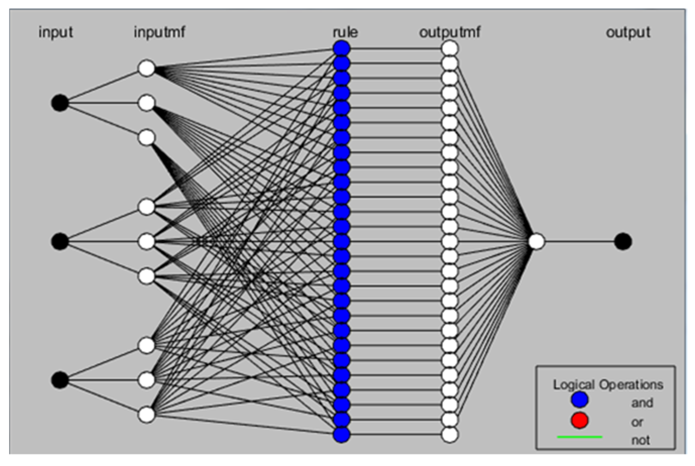
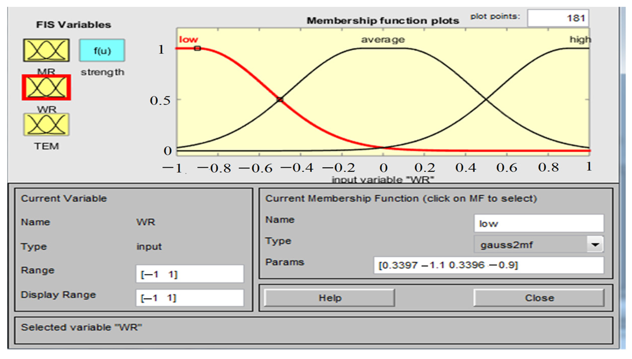
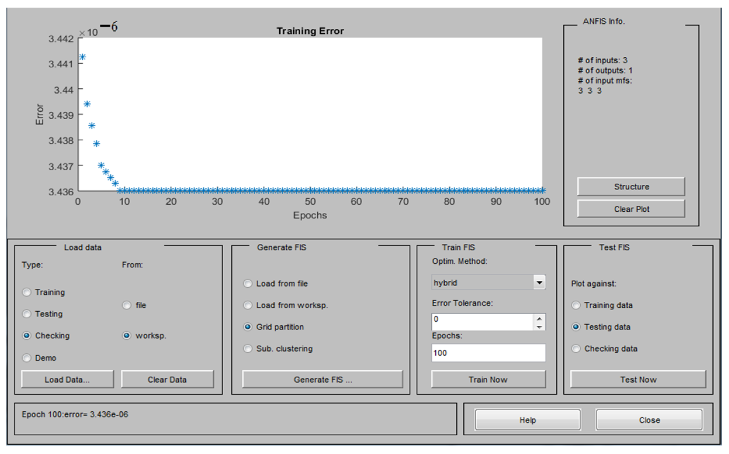
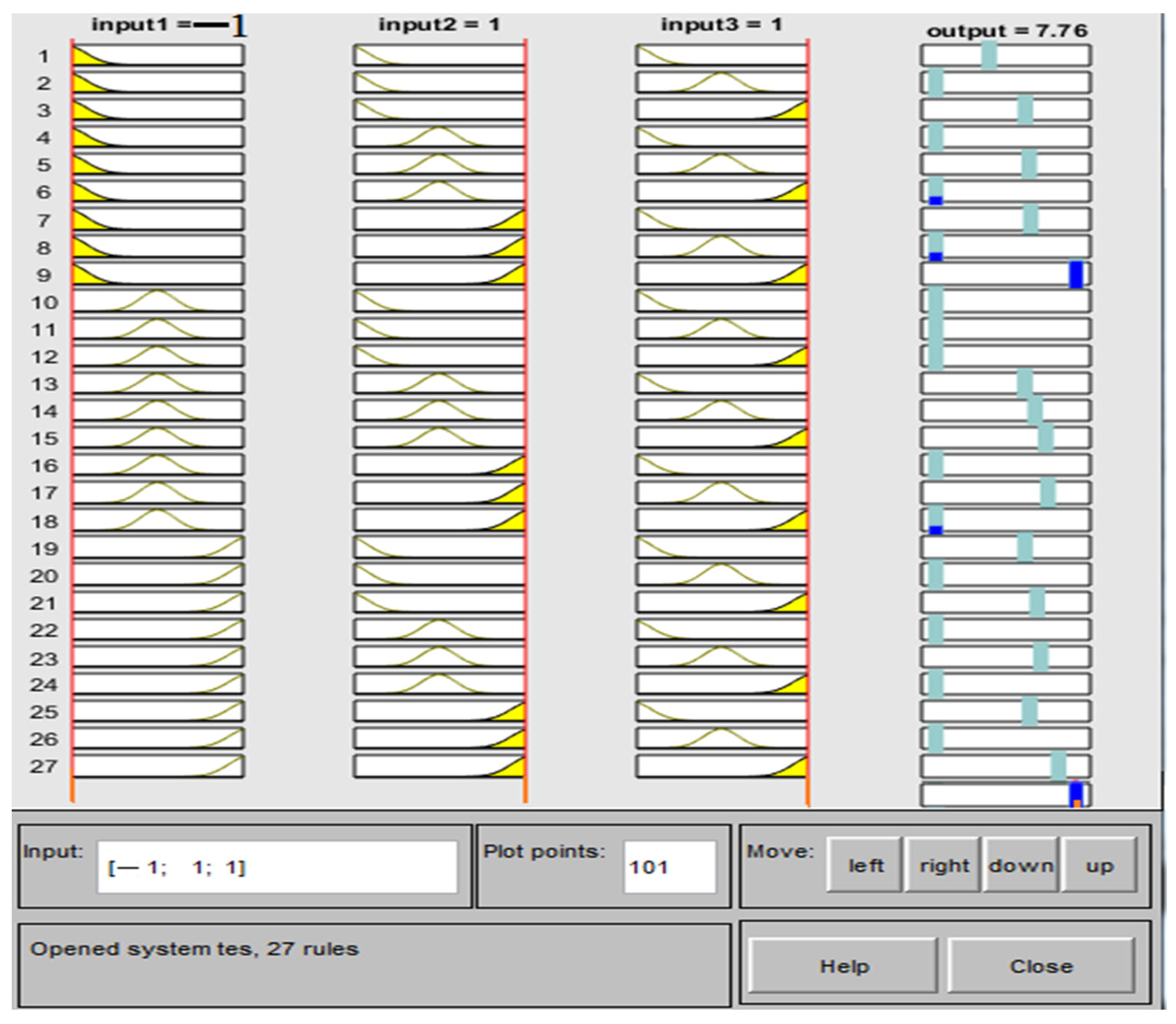
2.4.1. Adaptive Neuro-Fuzzy Inference System (ANFIS)

ANFIS is a universal approximation methodology that is able to approximate any real continuous function on a compact series with any degree of precision. The system offers a multi-input, single-output (MISO) fuzzy Sugeno model and a series of IF-THEN fuzzy rules entered in a framework of adaptive systems to adapt and facilitate training. The model was developed to predict the bonding strength of glulam using ANFIS, taking three input variables and one output variable into account. The architecture of the proposed model is presented in Figure 1 and is a combination of viz. fuzzification, product, rule or normalization, defuzzification and overall output layers. Assuming that the fuzzy inference system (FIS) being examined has the inputs (x,y) and the output (f), the IF-THEN fuzzy rules are used as follows:
R u l e   1 : I F   x   i s   P 1   a n d   y   i s   Q 1 ,   T H E N   f 1 = a 1 x + b 1 y + c 1
R u l e   2 : I F   x   i s   P 2   a n d   y   i s   Q 2 ,   T H E N   f 2 = a 2 x + b 2 y + c 1
R u l e   n : I F   x   i s   P i   a n d   y   i s   Q i ,   T H E N   f i = a i + b i y + c i
where P1…Pi and Q1…Qi are the fuzzy sets; f1…fi are the system’s outputs that are normally polynomial functions of the input variables for the inputs x and y; and a1…ai, b1…bi and c1…ci are adjustable parameters. This type of IF-THEN rule is called the “Sugeno fuzzy model” [35].
Since the FIS system is composed of five layers and the first layer includes three input variables, with all adaptive nodes are in this layer, each node (i) in this layer has a node function:
O i 1 = μ p i x i
where x is the input variable for node i, O1i is the membership grade of a fuzzy set (Pi) and determines a range in which the input x meets the quantity P and μpi is the membership function (MF). Gaussian2mf, a famous membership function was chosen, which is expressed as follows:
μ p i = e x c 2 2 σ 2    
where c and σ are the parameters of the Gaussian2mf theorem. MFs range from −1 to +1.
In the second layer (the product layer), all nodes are non-adaptive. This layer is used to check the weight of each MF and is the product of all received signals:
Q i 2 = w i   = μ P i x i   .   μ Q i x i ,     i = 1 , 2 .
The output of each node signifies the firing strength of weight and rule.
In the third layer including the normalization or rule layer, each node performs adaptation as a precondition of the fuzzy rules by calculating the activation level of each rule. The layer is the ratio of the firing strength of the rule relative to the total firing strength of the rules. It is also non-adaptive:
O i 3 = w i = w i w 1 + w 2 ,     i = 1 ,   2 .
The fourth layer is known as the defuzzification layer and is used to defuzzify the MFs to achieve the output. The centroid defuzzification method was used, which calculates the centroid of the region under the MFs. All nodes in this layer are adaptive with the following function:
O i 4 = w i . f i = w i a i x + b i y + c i
where {ai,bi,ci} is the set of the consequent parameters.
The fifth layer showing all outputs of all input layers of the fourth layer is a single node that is non-adaptive and described as follows:
O i 5 = i w i . f i = i w i . f i i w i
All ANFIS modeling was performed using the fuzzy logic toolbox of MATLAB R2015b (Mathworks Inc., Natick, MA, USA).
Least squares estimation was used to identify the next parameters. The error rates are propagated backward, while the premise parameters are updated when the gradient is descended. Then, the membership function of the ANFIS models was developed using optimization algorithms according to their counterparts in nature, such as ACOR, PSO, DE and GA, to ensure the bonding strength prediction error.

2.4.2. Ant Colony Optimization (ACOR)

ACOR algorithms have a wide range of applications due to their ability to solve both static and dynamic problems. These algorithms use a discrete structure to determine the solution. The discrete structure concept in an ACOR means that each decision variable is divided into a certain number of states within a defined range. In order to ensure that the variable space is discrete, a limitation is imposed on the algorithm that decreases the optimality precision. However, by dividing the space between the decision variables to a large degree, the solution precision is increased, and the program time increases accordingly. Furthermore, as the system becomes more complicated, the precision may decrease. To solve this problem, ACOR was generalized in the continuous space so that the algorithm would move in the R space and the continuity would be met using a probability density function. Socha and Dorigo proposed the Gaussian function. A Gaussian function cannot create several maxima [36]. Therefore, the kernel Gaussian function (sum of single Gaussian functions) was used, which is defined for the i-th decision variable as follows:
f i x = l k w l g i l x = l = 1 k w l 1 2 π σ i l exp x μ i l 2 σ i l 2
During the implementation of the algorithm, the parameters wl, μli and σli must be defined, and k is the number of single Gaussian functions. The decision variables related to the i-th solution are denoted by bl1 and bl2, and the n-th decision variable is denoted by bln, the value of which is calculated for each solution (h(bl)). The number of solutions is k. Then, the solutions are arranged in descending order based on quality and are saved. Then, for each bl, a weight (w) is determined, the value of which is proportional to the quality of the related solution, where w1w2 ≤ … ≥ wk is calculated as follows:
w l = 1 q p 2 π e x p l 1 2 2 q 2 k 2
If the value of q is assumed to be very small, it is less likely to select the weak solutions, and if it is excessively small, it falls within the local optimum. μli is equal to bll for the solution l and the i-th variable. σli is the standard deviation between all k values of the i-th variable relative to bli and is calculated as follows:
σ i l = ϑ z = 1 k b i e b i l k 1 ,   i = 1 , , m .
The coefficient ϑ is an adjustable parameter. The larger its value, the lower the convergence speed will be. The coefficient affects the long-term memory of the algorithm and makes it less likely that worse solutions are chosen, clearing them from the memory [36].

2.4.3. Particle Swarm Optimization (PSO)

PSO is a computational framework for continuous and discrete decision processes [37] that is based on the natural behavior of living creatures such as fish in their search for food resources. The main problems encountered in swarm optimization are accompanied by the position of N particles assigned randomly as a swarm in D-dimensional space. Each solution in the swarm is accompanied by a position, and each particle in the solution space is computed by a scoring function describing the problem status [38]. All particles find the best global position in the solution space and obtain the best personal positions [39]. The new identified position and the velocity of particles are updated according to the following rules [40]:
p = p + v
with
v = v + c 1 . r a n d . p b e s t p + c 2 . r a n d . g b e s t p
where p and v are the particle’s position and direction, respectively; c1 is the local weight; c2 is the global weight; pbest and gbest are the best positions of particles and swarms, respectively; and rand is a random value.

2.4.4. Differential Evaluation (DE)

DE was used as an intelligent optimization framework, whereby the basic optimized mutation, crossover and selection operators are imitated. DE relies on the D-dimensional parameter vectors and population size (NP) because it is a parallel direct search method and is not affected by the minimization processes; hence, the method is considered a population process when producing each generation (G). In DE, an initial population vector is selected to cover all parameter spaces; a uniform probability distribution is assigned to all random selections. DE produces new parameter vectors based on the accessible preliminary solution by producing the weight difference between two population vectors and a third vector through a mutation operation as follows:
x i , G = x 1 , i , G , x 2 , i , G , x n , i , G ,           i = 1 ,   2 , , k ,
where x1, G, i = 1,2,3,…,NP are the mutant vectors produced by applying νi,G + 1, and r1, r2 and r3 are the arbitrary selection numbers ∈[1,2,3,…,]…NP. The trial vector is determined by a combined process (crossover operation) that uses a combination of the mutated vector parameters and other predetermined vector parameters:
x L j x j ,   i , 1 x U j ,
where Uj,G + 1 is the trailer vector, xi,G is the target vector, rand b(j) denotes the j-th uniform random evaluation (∈∈[0,1]), rnbr(i) is a random value index (∈∈[1,2,3,…,d]) and CR is a crossover constant determined by the user. Finally, the trial vector is used as the target value of the next generation in the selection process and offers the lowest-cost function value compared to the target vector. Since each population must act as the target vector, NP tasks are considered a single generation procedure.

2.4.5. Genetic Algorithm

The GA is a directional random optimization method moving toward the optimum point gradually. One of the benefits of this algorithm is its very good global search that is independent of the problem status. It offers suitable performance combined with problems with large computations and does not fall within the local optimum [41]. ANFIS models including two types of parameters (i.e., antecedent and consequent parameters) that are tuned by gradient-based methods including the steep descend error (SDE) and the least square error (LSE). The solutions of the gradient-based method may fall within the local optimum. Therefore, the application of metaheuristic algorithms including GA with a random search nature can be a suitable alternative method. The antecedent parameters {σi, ci} or μpi in Equation (5) are related to the membership functions that can be optimized by the evolutionary algorithms. Any of these parameters contains N genes, where N is the number of the membership functions. The consequent parameters {Pi, Qi, ci} in Equation (3) can be trained by the optimization algorithm. In the Results section, the genes (I + 1) × R produce each chromosome. The objective function of the evolutionary algorithms used is the root mean square error (RMSE). To solve the mentioned optimum problem using the ANFIS-GA, the weight (μpi) of the fuzzy antecedent parameters is tuned by the GA algorithms like linear parameters such as Q, P and c.

2.5. Performance Evaluation

To determine the performance of each model, four statistics, i.e., the determination coefficient (R2), root mean square error (RMSE), mean absolute error (MAE) and sum square error (SSE), were used to analyze the performance of the new models in the following examined forms:
R 2 = i = 1 n x i x ¯ y i y ¯ / i = 1 n x i x ¯ 2 i = 1 n y i y ¯ 2 2
R M S E = 1 n i = 1 n x i y i 2
M A E = x i x ¯ n
S S E = i = 1 n x i x ¯ 2
where n is the number of observations; xi and x ¯ are the observed and mean values, respectively; and yi and ȳ are the related predicted and mean values, respectively. As R2 increases and approaches 1, the predicted values approach the experimental values, showing the high performance of the model in predicting the response with high precision. As the errors decrease to a minimum, the model under examination offers a more precise prediction of the response being examined.

3. Results and Discussion

Owing to the need for fewer runs in less time and the independence of the selected design, as well as the rotatability and generalizability of the results in infinite ranges, the central composite design (CCD) implemented in the RSM environment was used to determine the effect of the combination of the input variables on the dependent variable (bonding strength) up to 34 runs (Table 2).

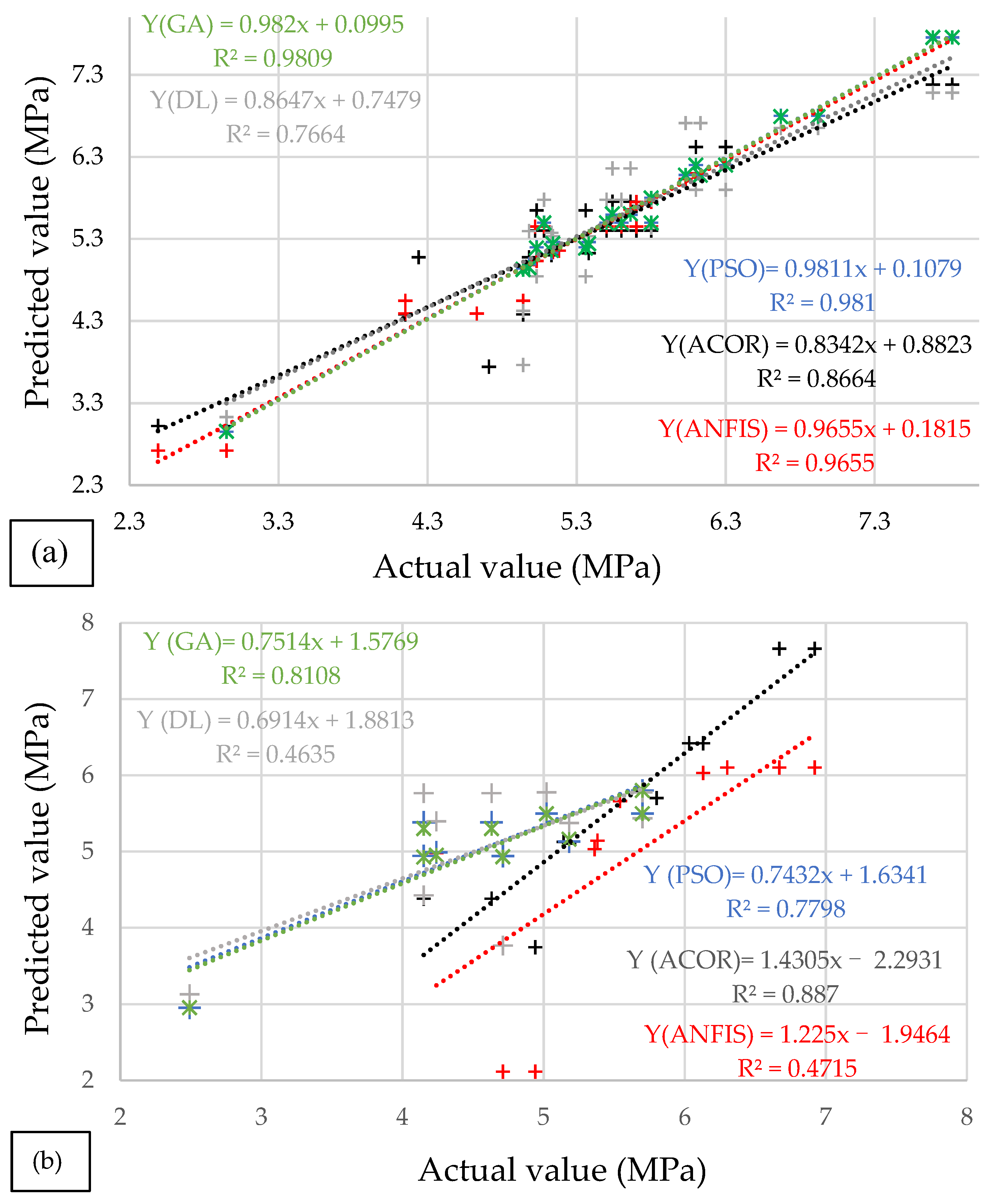
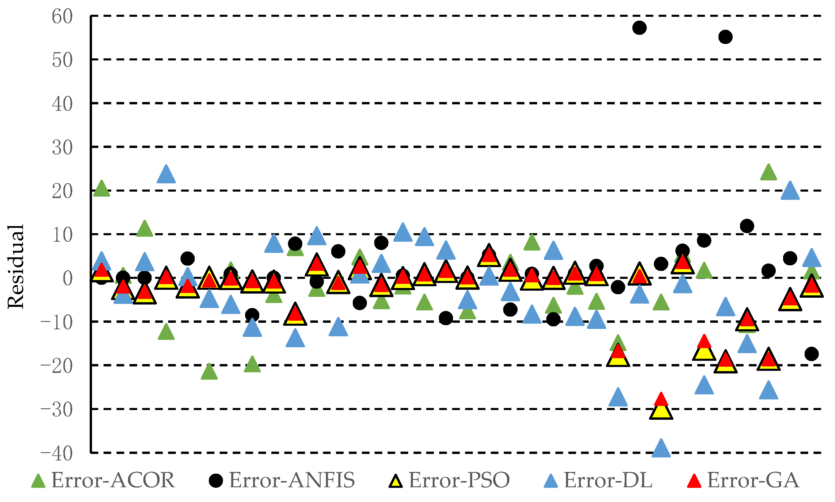
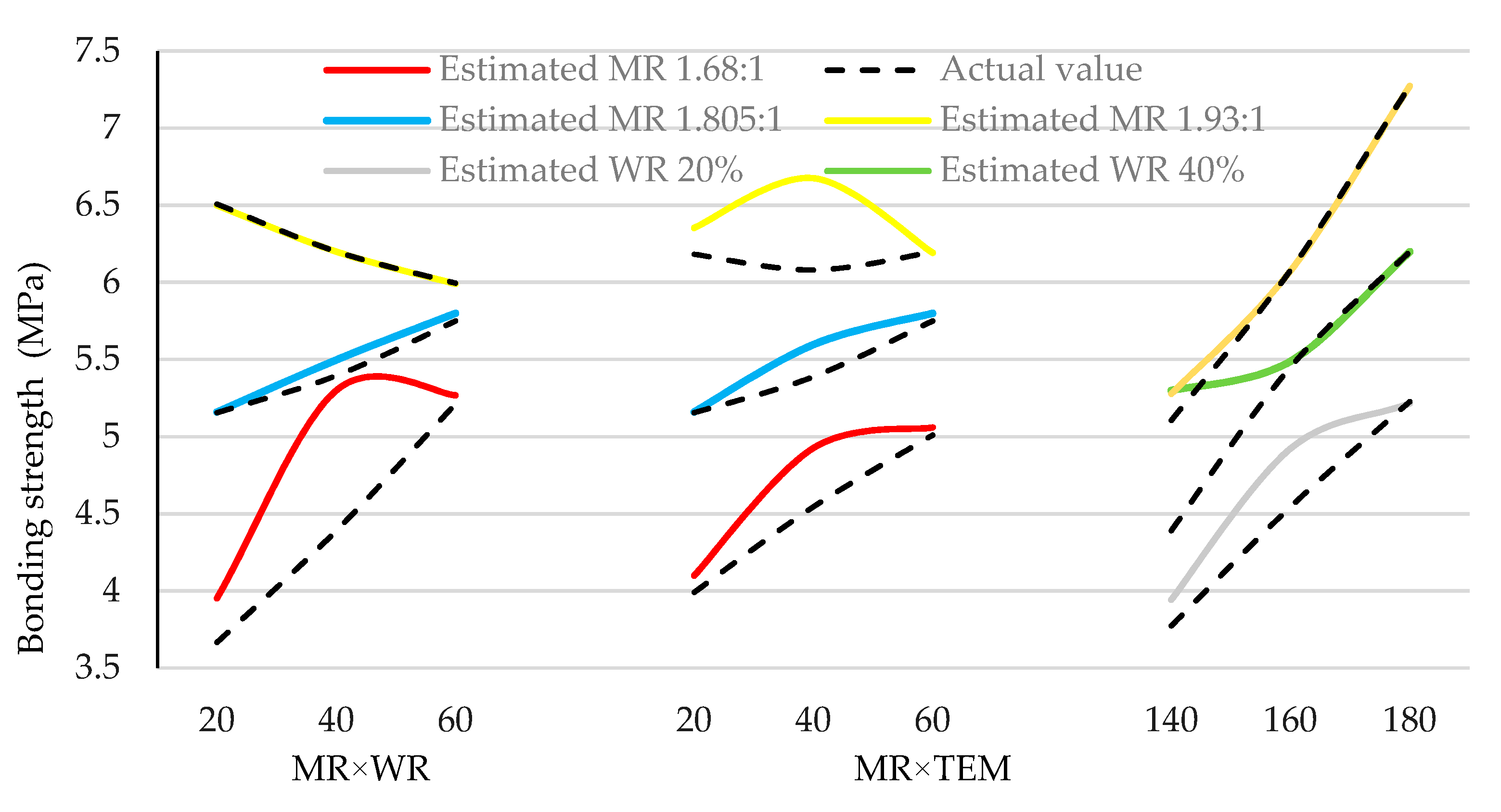
3.1. Accuracy of the Predicted Values Obtained by the Approaches

To determine the accuracy of the performance of the models used to estimate the output, the regression diagram of the experimentally measured values versus the values predicted by the ANFIS-based, ANFIS-ACOR, ANFIS-PSO, ANFIS-DE and ANFIS-GA models is given in Figure 2 for the training and testing datasets. The points distributed around the fit line represent the experimental data and include different matches between the models’ outputs and actual values. It is easily observed that, with a determination coefficient (or correlation coefficient) close to 1, the ANFIS-GA model produces less error compared to other models, making it more suitable to predict the bonding strength both for the training and test datasets.
Finally, while the ANFIS-GA model offers a better bonding strength prediction compared to other models, this model was preferred to develop the bonding strength at different MR, WR and Tem values. Using the well-trained ANFIS-GA model, the effect of the input data on the response in the related ranges was examined. The ANFIS-GA model has an R2 equal to 0.9809 for the training dataset and 0.8108 for the testing datasets, meaning that the model achieved excellent training of the outputs so that 98.09% and 81.08% of the estimated values agree with the measured values for the training and testing datasets, respectively.
In addition to R2, three other statistical indices that compare the deviation between the actual and estimated values, i.e., RMSE, MAE and SSE, are given in Table 3 to compare the performance of the developed prediction models. In addition to confirming the higher precision of the ANFIS-GA model to predict the output using R2 (Figure 2), the errors estimated by RMSE, MAE and SSE have lower values (0.3366, 0.2082 and 3.8523, respectively) than the ANFIS (0.7192, 0.3575 and 17.5885, respectively), ANFIS-ACOR (0.4711, 0.3636 and 7.5470, respectively), ANFIS-DE (0.6157, 0.4905 and 12.8904, respectively) and ANFIS-PSO (0.3535, 0.2135 and 4.2479, respectively) models. Using different hybrids of the ANFIS model, the errors were decreased, with the most limited decrease associated with the using the GA model (Figure 3). More than 70% of the errors produced range from −5% to 5% in the model developed with the GA, while in the basic ANFIS and ACOR models, the errors are distributed in a wider range from −40% to 60%. Hence, the hybrid ANFIS-GA model can be used to predict the response values with the highest precision among tested models. The random division of data into two testing and training phases led to an overfitting problem because the classic training algorithms are generally very dependent on the training datasets and cannot offer an acceptable performance in the testing phase (Figure 3). Unlike the classic ANFIS model, the hybrid ANFIS algorithms showed reliable performance in the testing and training phases. The best hybrid methods prevent the system from falling into overfitting and local optima [42]. The performance of the GA method may be due to the ability of the algorithm to model a complex phenomenon. The weak performance of other optimization methods such as PSO may be due to the weakness of the algorithms to solve hard problems compared to GA [43] because the simple PSO structure cannot precisely optimize the bonding strength values. Furthermore, the classic ANFIS model that uses gradient-based training techniques including backpropagation requires many burden values to be optimized and trained when the number of inputs is increased [41].
As mentioned in the previous section, the overfitting problem is very common among the problems encountered when mathematically solving datasets. This suggests that a model may be successful in an excellent simulation of the data used to develop and train it, but at the same time, the model may predict very abnormal values for the values of the input parameters except those used in the development and training process [44]. Hence, it is necessary to compare the results of the tested methods with the experimental values or results similar to those reported in other studies in which a wide range of input parameter combinations affects the response. In the first, second and third cases of experimental verification, the bonding strength related to the MR, WR and Tem of the obtained experimental results was tested (Figure 4). For the first input parameter (MR), overfitting occurred in the ANFIS-based and hybrid ACOR, PSO and DE models. Overfitting was stronger for the simulation of the ANFIS and hybrid DE datasets, while no overfitting occurred when using the GA. For the second parameter (WR), no overfitting occurred when using the hybrid GA for modeling, while overfitting clearly occurred when other methods were applied, with the strongest overfitting associated with the ANFIS-based and other hybrid models, although weaker compared to the MR effect. For the third input parameter, the changes in the overfitting were similar to the effect due to the application of the second input parameter. In other words, the GA has minimum overfitting, while the overfitting occurred to some extent with the application of the other tested models. The changes in the overfitting of the WR and Tem parameters follow a similar pattern, although the changes in overfitting are much less than the MR effect.
ANFIS is an intelligent neuro-fuzzy method used to model and control uncertain systems. ANFIS considers both input and output data. The proposed ANFIS structure is used to model the prediction system including the determination/preparation of the input and output values, determination/examination of the fuzzy sets for input variables, identification of the fuzzy rules and creation and training the neural network. It requires development of a means to implement and test the proposed structure in order to produce and evaluate fuzzy systems using a graphical user interface (GUI). This tool contains an FIS editor, MF editor, rule editor, output surface viewer and fuzzy interface viewer. The FIS editor provides general information about the FIS, while the MF editor edits and shows MFs accompanied by all input and output variables. The rule editor allows for the creation of rule expressions in an automatic route by clicking and choosing one case in each input variable frame, one item in each output frame and one connection item. Using the rule viewer, the user can completely interpret the fuzzy inference process each time. In the ANFIS editor, the GUI selection panel initializes the FIS training, saves the FIS object and opens a Sugeno schema for FIS interpretation. In the MF design, a Gaussian or bell-shaped MF was used to develop the fuzzy models due to its flexibility and simplicity. The modeling results were developed based on the Gaussian MF, which was selected as the best among all tested MF types (Figure 5). Figure 5 shows the Gaussian MFs of the input parameters by the developed ANFIS-GA model to predict the bonding strength of glulam. Each input parameter with three MFs showed the best result in predicting the bonding strength of glulam. Hence, a set of 27 fuzzy rules (3 × 3 × 3) was designed by the system to solve the problem. Low, average and high qualitative variables were employed in the modeling process. Moreover, the output MF type was assumed to be linear. In the developed hybrid ANFIS-GA model, no change was observed in the network performance after epoch № 9 (Figure 6). As shown in Figure 6, the FIS + ANFIS_gauss2 model achieved the best prediction performance results, followed by the FIS + ANFIS_gauss, FIS + ANFIS_Bell and FIS + ANFIS_Trap models. During training for many epochs, the error tolerance was set at zero, while a maximum band was not considered for the number of epochs. The error saturation was determined as the final result of the training period [45]. When the error was constant, the training stopped and was considered the training saturation point. It is worth noting that all datasets were divided into two separate training (80% of all datasets) and testing (20% of all datasets) sets to develop and evaluate the model. After training by ANFIS-GA, the dataset was tested using the hybrid and subclustering algorithms with different membership functions. While the hybrid method uses the backpropagation algorithm for all input membership functions and the least square algorithm for the output membership functions simultaneously and according to the prioritization of different membership functions, the fuzzy system was created with rules to differentiate the fuzzy quality accompanied by each cluster. In the rule-framing process, the functions NOT, OR and AND were used, as shown in Figure 1.

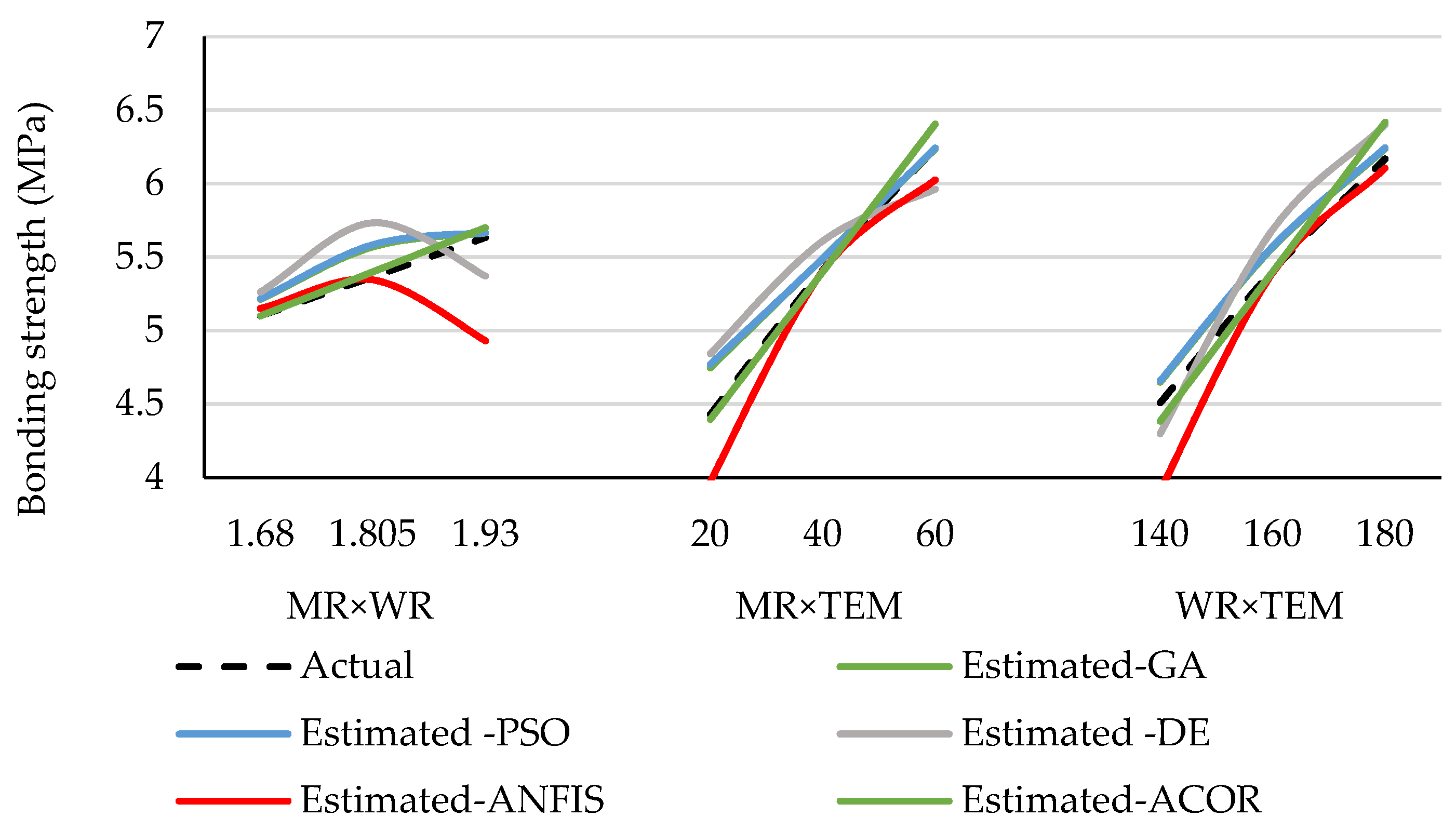
3.2. Optimized Values of the Preferred Approach

To better synthesize and understand the fuzzy response behavior, the rules were evaluated (Figure 7) using the selected ANFIS-GA model. Figure 7 shows the rule viewer indicating different input values in the model and the calculated output. The bonding strength (output) can be predicted by changing the parameters, including MR, WR and Tem, for the chosen and developed ANFIS model. In this regard, to determine the interactive effect of the parameters on the outputs and based on the GA model, the change in the value of each parameter can be presented as a graph. It is observed that when the parameters were changed so that MR was minimum (1.68:1:1), WR was maximum (60%) and the press temperature was maximum (180 °C), the bonding strength reached a maximum value (7.76 MPa).
Figure 8 also represents the interactive effect of the investigated parameters on the output and the graphical difference relative to the actual values of the response. Figure 9 also shows the interactive effect of the parameters on the output. As shown in Figure 8, the general changes in the strength follow a unique pattern when comparing the real values with the estimated values, except the effect of the molar ratio of 1.68:1 in the interaction with WR on the estimated strength, the molar ratio of 1.93:1 in the interaction with the Tem on the estimated strength and WR 20% in the interaction with Tem on the estimated strength, which is inconsistent with the changes in the experimental strengths when using the same parameters.
Figure 8 and Figure 9 represent conditions under which the third parameter is fixed in the middle of the value range. The diagram of the interactive effects was generated based on statistical analysis of the GA, showing that the interactive effects on the bonding strength including MR × WR, MR × Tem and WR × Tem were statistically significant according to ANOVA.
As shown Figure 8 and Figure 9a, as the WR increases to a maximum value, the MR decreases to a minimum value, the strength increases to a maximum value and Tem is maintained at a median value (160 °C). As WR decreases to a minimum value and MR increases to a maximum value, the strength also increases but not reach a maximum. In other words, there is an inverse relation between MR and WR. The minimum value of the strength is also reached as both MR and WR decrease.
As shown in Figure 8 and Figure 9b, as MR and Tem increase, the strength increases and approaches the maximum level, but the maximum value of the strength occurs when MR is minimum, and the Tem is maximum. Comparison of Figure 9a,b shows that in both cases, an increase in MR results in an increase in the strength, while the decreasing effect of the increase in the Tem is much less than the decreasing effect of the increase in MR. This means that when applying higher values of WR, a higher range of temperature can be used to compensate for the decreasing effect of MR.
The interactive effect of WR and Tem on the strength is shown in Figure 8 and Figure 9c. As the Tem and WR increase simultaneously when the MR is at a median value (1.805:1), the strength reaches a maximum value. However, as both parameters decrease to minimum values, the strength also reaches its minimum.
Protein contains strong polar groups such as hydroxyl, amide and carboxyl. Since the components of wood such as cellulose, hemicellulose and lignin are polar, the main molecular forces between the wood surface and protein are the interactions of the polar groups. As protein is treated by NaOH, the internal hydrogen bonds of the coiled protein molecules break and open widely and are exposed to many accessible polar groups, making connection possible. During the treatment, the produced peptide chain contributes to the bondability with a suitable molecular weight distribution [46]. The constancy of viscosity in all ranges of the shear rate, i.e., Newtonian fluid, occurs due to the small size of UF molecules and disorientation with the shear flow. According to the non-Newtonian behavior of a protein suspension [47], shear-thinning behavior is possible for the MUF/MP adhesive in which modified proteins play the role of a rheological modifier. Hence, owing to the increase in the protein–water interaction through hydrogen bonds, the viscosity increases. At lower levels of protein, the distance between random coils is more than the radius of gyration so that no entanglement occurs, and the suspension’s viscosity is comparable to that of its solvent. As protein content increases, the relative viscosity increases gradually to a threshold (*C) at which the distance between the random coils (d) is almost equal to the radius of gyration, beyond which the relative viscosity suddenly increases exponentially. When the suspension concentration (C) increases beyond the critical concentration (*C), polymer entanglement becomes dominant, and viscosity increases exponentially [48]. In this process, pseudoplastic behavior occurs even at low ratios of protein [49], and overpenetration is avoided as viscosity increases.
The structural changes of the adhesive compound indicate that the modulus of elasticity (G’) and viscous modulus (G”) are functions of shear stress in the stress–strain curve accompanied by the sample’s strength against the fluid ability [49], indicating the structural stability of the material [50]. The modulus (G’) is significantly lower in UF than adhesive containing protein. UF exhibiting pseudo-liquid behavior can be expressed by the relation G” > G’, while protein showing pseudo-gel behavior can be expressed by G’ > G”. This phenomenon is due to the formation of an entangled network in the presence of protein, promoting the structural strength of the suspension. This behavior is promoted by protein denaturation by adding NaOH, which increases the random coil volume of the polymer [51]. The rheological behavior of the UF/modified protein compound shows the entangled structure of the sample even at low levels of protein (G’ > G”), and G’ is almost aligned with modified protein alone in the linear region of the stress–strain curve of the UF/modified protein compound. Hence, all rheological properties of the adhesive compound are affected by the presence of high-molecular-weight protein. Hence, the protein and UF resin chain can be interwoven to achieve crosslinking during and even after pressing [52].
After curing, UF has smooth surfaces, as a thermoset polymer has a brittle form during failure [53,54]. Brittle rupture means that no ductile rupture has occurred during the test. However, as an adhesive is added with no brittle rupture, the rupture range is added in the stress–strain curve, and the viscous deformation range is added during the rupture test. Such a change in the rupture curve was observed during the test in practice. Bacigalupe et al. also observed ductility in an adhesive when adding protein to UF [49]. Such a ductile rupture that can show that a crosslinked network exists between the UF and that modified protein does not exist in the cured non-modified protein adhesive [55]. However, in the UF/protein adhesive, ductility increases as the modified protein increases [49], and practical observations in the tests indicated that no phase separation occurred, demonstrating the compatibility of the two components.
As a denaturing agent, urea breaks the globular structure of the protein into short protein chains and increases its viscosity. In this process, a secondary structure of protein forms through the reaction between oxygen and urea hydrogen atoms and hydroxyl groups of protein [56], leading to bonding and solubilization. The increase in solubilization allows the protein to flow better on the wood and forms hydrogen bonds with wood, producing subsequent chemical crosslinkings [57]. Meanwhile, denaturation intensifies when the reaction intensity increases such as by applying a higher press temperature, increased pressure, a change in pH or adding urea [58,59].
According to the endothermic reaction during the change in the natural protein state to the denatured state in the temperature range of 160–175 °C [4] followed by crosslinking of the MUF resin methylol groups with amino bonds, amide bonds and naturated or denaturated protein, a sufficiently high press temperature further denatures the modified protein and enables a reaction with fibers. The polar functional groups in the protein and carbohydrates such as hydroxyl, amino and carboxylic acid can react with formaldehyde and form bonds with each other with a high energy level of wood [60,61].
Due to the high moisture content in the modified protein, as MUF is applied with a higher formaldehyde molar ratio, an insufficient adhesive curing reaction is produced, preventing the complete polycondensation of MUF resin [34] because the urea and melamine percentages are decreased to simultaneously make connections with formaldehyde and modified protein. In addition, the curing time of the modified MUF resin is increased because the reactivity of the MU/protein adhesive decreases as protein content increases [62]. Under these conditions, adding protein can positively affect the completion of more copolymerization reactions by moving the equilibrium shift forward [63]. At the same time, as a result of the increase in moisture due to the increase in modified protein (WR), the force resulting from the saturated vapor pressure easily exceeds the internal bonding force of the glue line. Hence, in addition to the prevention of additional involvement of urea, melamine or protein with formaldehyde followed by additional release of free formaldehyde, the bonding strength decreases because moisture can create gaps due to the formation of steam and produce a rough surface on the glue line [64].
Based on the hypothesis related to the unfolding of protein molecules and their breakdown into smaller pieces, the active groups were exposed after NaOH hydrolysis treatment through the destruction of the van der Waals force, hydrogen bonds and hydrophobic interaction between the molecules in the protein. In this process, the exposed active amine can react with formaldehyde and form hydroxymethyl. Hydroxymethyl can react with urea, urea methylol, amine or hydroxymethyl under the final acidic conditions used in the glue line to form methylene and ether methylene bridges and produce chains with random crosslinkings with each other to form a 3D structure after curing [63]. Under these conditions, no hole or crack is produced, and the surface becomes smooth during the rupture as a result of the use of unfolded protein molecules and rearrangement, together with denaturation and the formation of a more crystalline matrix with a smoothened surface [64].
Adding even a small amount of protein causes a sharp decrease in the solid content of the adhesive. Simultaneously, due to the increase in viscosity resulting from the addition of formaldehyde, the solid content decreases [65]. However, as the F-to-U/M molar ratio decreases according to urea/melamine properties to unfold the globular structure of protein, the increase in the U/M molar ratio increases the solid content and it limits the need for additional time. According to the low solid content in the presence of protein, as the press temperature increases and to remove the superfluous water from resin to avoid delamination of the board, the bonding strength improves [65].

4. Conclusions

In the present study, basic ANFIS, ANFIS-ACOR, ANFIS-PSO, ANFIS-DE and ANFIS-GA models were developed to predict the bonding strength of glulam made with MUF-modified soy protein adhesive. A three-factor, three-level CCD design was used to make the test samples to compare the prediction precision of the response under examination obtained by all applied methods. After designing and testing the systems, the predictability of all five models was compared using statistical criteria, i.e., R2, RMSE, MAE and SSE. After determining the best model in terms of precision in estimating the response, it was used to determine the optimum level of the variables used to achieve the highest bonding strength. The results indicate that by combining the basic ANFIS model with other algorithms, the accuracy of the response estimation can be generally increased. The combination of the genetic algorithm with the ANFIS model resulted in a more accurate response estimation compared to combinations with other algorithms, with an R2 of 0.9809, RMSE of 0.3366, MAE of 0.2082 and SSE of 3.8523. Hence, the optimization method has had a higher prediction accuracy. Based on the developed model, the optimum input values to produce glulam with a maximum bonding strength (7.76 MPa) were a minimum MR value (1.68:1), a maximum WR value (60:40) and a maximum press temperature value (180 °C).

Author Contributions

Conceptualization, methodology, software, validation, formal analysis, investigation and resources, project administration, writing and original draft preparation, M.N. and F.N.; investigation, visualization, writing—review and editing and supervision, A.N.P. All authors have read and agreed to the published version of the manuscript.

Funding

This research received no external funding.

Data Availability Statement

The data presented in this study are available on request from the corresponding author.

Conflicts of Interest

The authors declare no conflict of interest.

References

  1. Cheng, H.; Dowd, M.K.; He, Z. Investigation of modified cottonseed protein adhesives for wood composites. Ind. Crops Prod. 2013, 46, 399–403. [Google Scholar] [CrossRef]
  2. Kumar, R.; Choudhary, V.; Mishra, S.; Varma, I.K.; Mattiason, B. Adhesives and plastics based on soy protein products. Ind. Crops Prod. 2002, 16, 155–172. [Google Scholar] [CrossRef]
  3. Hettiarachchy, N.; Kalapathy, U.; Myers, D. Alkali-modified soy protein with improved adhesive and hydrophobic properties. J. Am. Oil Chem. Soc. 1995, 72, 1461–1464. [Google Scholar] [CrossRef]
  4. Yang, G.; Yang, B.; Yuan, C.; Geng, W.; Li, H. Effects of preparation parameters on properties of soy protein-based fiberboard. J. Polym. Environ. 2011, 9, 146–151. [Google Scholar] [CrossRef]
  5. Taghiyari, H.R.; Hosseini, S.B.; Ghahri, S.; Ghofrani, M.; Papadopoulos, A.N. Formaldehyde emission in micron-sized wollastonite-treated plywood bonded with soy flour and urea-formaldehyde resin. Appl. Sci. 2020, 10, 6709. [Google Scholar] [CrossRef]
  6. Pereira, F.; Pereira, J.; Paiva, N.; Ferra, J.; Martins, J.M.; Magalhaes, F.D.; Carvalho, L. Natural additive for reducing formaldehyde emissions in urea-formaldehyde resins. J. Renew. Mater. 2016, 4, 41–46. [Google Scholar] [CrossRef]
  7. Sun, X.; Bian, K. Shear strength and water resistance of modified soy protein adhesives. J. Am. Oil Chem. Soc. 1999, 76, 977–980. [Google Scholar] [CrossRef]
  8. Huang, W.; Sun, X. Adhesive properties of soy proteins modified by urea and guanidine hydrochloride. J. Am. Oil Chem. Soc. 2000, 77, 101–104. [Google Scholar] [CrossRef]
  9. Yapici, F.; Senyer, N.; Esen, R. Comparison of the multiple regression, ANN, and ANFIS models for prediction of MOE value of OSB panels. Wood Res. 2016, 61, 741–754. [Google Scholar]
  10. Alhijazi, M.; Safaei, B.; Zeeshan, Q.; Asmael, M.; Harb, M.; Qin, Z. An experimental and metamodeling approach to tensile properties of natural fibers composites. J. Polym. Environ. 2022, 30, 4377–4393. [Google Scholar] [CrossRef]
  11. Nazerian, M.; Naderi, F.; Partovinia, A.; Papadopoulos, A.N.; Younesi-Kordkheili, H. Developing adaptive neuro-fuzzy inference system-based models to predict the bending strength of polyurethane foam-cored sandwich panels. Proc. Inst. Mech. Eng. Part L J. Mater. Des. Appl. 2022, 236, 3–22. [Google Scholar] [CrossRef]
  12. Papadopoulos, A.N. Advances in Wood Composites. Polymers 2020, 12, 48. [Google Scholar] [CrossRef] [PubMed] [Green Version]
  13. Wong, Y.J.; Mustapha, K.B.; Shimizu, Y.; Kamiya, A.; Arumugasamy, S.K. Development of surrogate predictive models for the nonlinear elasto-plastic response of medium density fibreboard-based sandwich structures. Int. J. lightweight Mater. 2021, 4, 302–314. [Google Scholar] [CrossRef]
  14. Jamali, F.; Mousavi, S.R.; Peyma, A.B.; Moodi, Y. Prediction of compressive strength of fiber-reinforced polymers-confined cylindrical concrete using artificial intelligence methods. J. Reinf. Plast. Compos. 2022, 41, 679–704. [Google Scholar] [CrossRef]
  15. Karaboga, D.; Kaya, E. Training ANFIS by using and adaptive and hybrid artificial bee colony algorithm (aABC) for the identification of nonlinear static systems. Arab. J. Sci. Eng. 2019, 44, 3531–3547. [Google Scholar] [CrossRef]
  16. Al-Musawi, A.A.; Alwanas, A.A.H.; Salih, S.Q.; Ali, Z.H.; Tran, M.T.; Yaseen, Z.M. Shear strength of SFRCB without stirrups simulation: Implementation of hybrid artificial intelligence model. Eng. Comput. 2020, 36, 1–11. [Google Scholar] [CrossRef]
  17. Jayaram, M.A.; Nataraja, M.C.; Ravi Kumar, C.N. Design of high performance concrete mixes through particle swarm optimization. J. Intell. Syst. 2010, 19, 249–264. [Google Scholar] [CrossRef]
  18. Flint, M.; Grünewald, S.; Coenders, J. Ant colony optimization for ultra high performance concrete structures. In Designing and Building with UHPFRC; Toutlemonde, F., Resplendino, J., Eds.; John Wiley & Sons: Hoboken, NJ, USA, 2011. [Google Scholar] [CrossRef]
  19. Quaranta, G.; Fiore, A.; Marano, G.C. Optimum design of prestressed concrete beams using constrained differential evolution algorithm. Struct. Multidiscipl. Optim. 2014, 49, 441–453. [Google Scholar] [CrossRef]
  20. Coello Coello, C.A.; Christiansen, A.D.; Hernández, F.S. A simple genetic algorithm for the design of reinforced concrete beams. Eng. Comput. 1997, 13, 185–196. [Google Scholar] [CrossRef]
  21. Elbaz, K.; Shen, S.L.; Sun, W.J.; Yin, Z.Y.; Zhou, A. Prediction model of shield performance during tunneling via incorporating improved particle swarm optimization into ANFIS. IEEE Access 2020, 8, 39659–39671. [Google Scholar] [CrossRef]
  22. Babanezhad, M.; Behroyan, I.; Nakhjiri, A.T.; Marjani, A.; Rezakazemi, M.; Shirazian, S. High-performance hybrid modeling chemical reactors using differential evolution based fuzzy inference system. Sci. Rep. 2020, 10, 21304. [Google Scholar] [CrossRef] [PubMed]
  23. Jing, H.; Rad, H.N.; Hasanipanah, M.; Armaghani, D.J.; Qasem, S.N. Design and implementation of a new tuned hybrid intelligent model to predict the uniaxial compressive strength of the rock using SFS-ANFIS. Eng. Comput. 2021, 37, 2717–2734. [Google Scholar] [CrossRef]
  24. Penghui, L.; Ewees, A.A.; Beyaztas, B.H.; Qi, C.; Salih, N.Q.; Al-Ansari, N.; Bhagat, S.K.; Yaseen, Z.M.; Singh, V.P. Metaheuristic optimization algorithms hybridized with artificial intelligence model for soil temperature prediction: Novel model. IEEE Access 2020, 8, 51884–51904. [Google Scholar] [CrossRef]
  25. Bui, Q.T.; Van Pham, M.; Nguyen, Q.H.; Nguyen, L.X.; Pham, H.M. Whale optimization algorithm and adaptive neuro-fuzzy inference system: A hybrid method for feature selection and land pattern classification. Int. J. Remote Sens. 2019, 40, 5078–5093. [Google Scholar] [CrossRef]
  26. Zhang, S.; Bui, X.N.; Trung, N.T.; Nguyen, H.; Bui, H.B. Prediction of rock size distribution in mine bench blasting using a novel ant colony optimization-based boosted regression tree technique. Nat. Resour. Res. 2020, 29, 867–886. [Google Scholar] [CrossRef]
  27. Jaafari, A.; Zenner, E.K.; Panahi, M.; Shahabi, H. Hybrid artificial intelligence models based on a neuro-fuzzy system and metaheuristic optimization algorithms for spatial prediction of wildfire probability. Agric. For. Meteorol. 2019, 266–267, 198–207. [Google Scholar] [CrossRef]
  28. Elbaz, K.; Shen, S.L.; Zhou, A.; Yuan, D.J.; Xu, Y.S. Optimization of EPB shield performance with adaptive neuro-fuzzy inference system and genetic algorithm. Appl. Sci. 2019, 9, 780. [Google Scholar] [CrossRef] [Green Version]
  29. Sari, P.a.; Suhatril, M.; Osman, N.; Muazu, M.A.; Katebi, J.; Abavisani, A.; Ghaffari, N.; Chahnasir, E.S.; Wakil, K.; Khorami, M.; et al. Developing a hybrid adoptive neuro-fuzzy inference system in predicting safety of factors of slopes subjected to surface eco-protection techniques. Eng. Comput. 2020, 36, 1347–1354. [Google Scholar] [CrossRef]
  30. Yaseen, Z.M.; Melini, W.H.; Mohtar, H.W.; Ameen, A.M.S.; Ebtehaj, I.; Razali, S.F.M.; Bonakdari, H.; Salih, S.Q.; Al-Ansari, N.; Shahid, S. Implementation of univariate paradigm for streamflow simulation using hybrid data-driven model: Case study in tropical region. IEEE Access 2019, 7, 74471–74481. [Google Scholar] [CrossRef]
  31. Varnamkhasti, M.J. A hybrid of adaptive neuro-fuzzy inference system and genetic algorithm. J. Intell. Fuzzy Syst. 2013, 25, 793–796. [Google Scholar] [CrossRef]
  32. Varnamkhasti, M.J. ANFISGA-adaptive neuro-fuzzy inference system genetic algorithm. Glob. J. Comput. Sci. Technol. 2011, 11, 15036870. [Google Scholar]
  33. Yuan, Z.; Wang, L.N.; Ji, X. Prediction of concrete compressive strength: Research on hybrid models genetic based algorithms and ANFIS. Adv. Eng. Softw. 2014, 67, 156–163. [Google Scholar] [CrossRef]
  34. Jiang, K.; Zhang, J.; Xia, S.; Ou, C.; Fu, C.; Yi, M.; Li, W.; Jing, M.; Lv, W.; Xiao, H. Improve performance of soy protein adhesives with a low molar ratio melamine-urea-formaldehyde resin. J. Phys. Conf. Ser. 2020, 1549, 032083. [Google Scholar] [CrossRef]
  35. Takagi, T.; Sugeno, M. Fuzzy identification of systems and its applications to modeling and control. IEEE Trans. Syst. Man. Cybern. 1985, 15, 116–132. [Google Scholar] [CrossRef]
  36. Socha, K.; Dorigo, M. Ant colony optimization for continuous domains. Eur. J. Oper. Res. 2008, 185, 1155–1173. [Google Scholar] [CrossRef] [Green Version]
  37. Kennedy, J.; Eberhart, R. A new optimizer using particles swarm theory. In Proceedings of the Sixth International Symposium on Micro Machine and Human Science, Nagoya, Japan, 4–6 October 1995. [Google Scholar]
  38. Liu, X.; Hussein, S.H.; Ghazali, K.H.; Tung, T.M.; Yaseen, Z.M. Optimized adaptive neuro-fuzzy inference system using metaheuristic algorithms: Application of shield tunnelling ground surface settlement prediction. Complexity 2021, 2021, 6666699. [Google Scholar] [CrossRef]
  39. Mohandes, M.A. Modeling global solar radiation using Particle Swarm Optimization (PSO). Sol. Energy 2012, 86, 3137–3145. [Google Scholar] [CrossRef]
  40. Catalao, J.P.S.; Pousinho, H.M.I.; Mendes, V.M.F. Hybrid wavelet-PSO-ANFIS approach for short-term electricity prices forecasting. IEEE Trans. Power Syst. 2011, 26, 137–144. [Google Scholar] [CrossRef]
  41. Shihabudheen, K.V.; Pillai, G.N. Recent advances in neuro-fuzzy system: A survey. Knowl. Based Syst. 2018, 152, 136–162. [Google Scholar] [CrossRef]
  42. Kisi, O.; Azad, A.; Kashi, H.; Saeedian, A.; Hashemi, S.A.A.; Ghorbani, S. Modeling groundwater quality parameters using hybrid neuro-fuzzy methods. Water Resour. Manag. 2019, 33, 847–861. [Google Scholar] [CrossRef]
  43. Azad, A.; Manoochehri, M.; Kashi, H.; Farzin, S.; Karami, H.; Nourani, V.; Shiri, J. Comparative evaluation of intelligent algorithms to improve adaptive neuro-fuzzy inference system performance in precipitation modelling. J. Hydrol. 2019, 571, 214–224. [Google Scholar] [CrossRef]
  44. Armaghani, D.J.; Asteris, P.G.A. Comparative study of ANN and ANFIS models for the prediction of cement-based mortar materials compressive strength. Neural Comput. Applic. 2021, 33, 4501–4532. [Google Scholar] [CrossRef]
  45. Mercy, L.J.; Prakash, S. Experimental investigation and neuro fuzzy modeling of inplane shear strength for self-healing GFRP. Transac. Ind. Inst. Met. 2016, 69, 1483–1491. [Google Scholar] [CrossRef]
  46. Wang, D.; Sun, X.S. Low density particleboard from wheat straw and corn pith. Ind. Crops Prod. 2002, 15, 43–50. [Google Scholar] [CrossRef]
  47. Bacigalupe, A.; He, Z.; Escobar, M.M. Effects of rheology and viscosity of bio-based adhesives on bonding performance. In Bio-Based Wood Adhesives; CRC Press: Boca Raton, FL, USA, 2017; pp. 293–309. [Google Scholar] [CrossRef]
  48. Chang, Q. Rheology Properties. In Colloid and Interface Chemistry for Water Quality Control; Elsevier: Amsterdam, The Netherlands, 2016; pp. 61–77. [Google Scholar] [CrossRef]
  49. Bacigalupe, A.; Molinari, F.; Eisenberg, P.; Escobar, M.M. Adhesive properties of urea-formaldehyde resins blended with soy protein concentrate. Adv. Compos. Mater. 2020, 3, 213–221. [Google Scholar] [CrossRef]
  50. Zhang, X.; Ding, Y.; Zhang, G.; Li, L.; Yan, Y. Preparation and rheological studies on the solvent based acrylic pressure sensitive adhesives with different crosslinking density. Int. J. Adhes. Adhes. 2011, 31, 760–766. [Google Scholar] [CrossRef]
  51. Bacigalupe, A.; Poliszuk, A.K.; Eisenberg, P.; Escobar, M.M. Rheological behavior and bonding performance of an alkaline soy protein suspension. Int. J. Adhes. Adhes. 2015, 62, 1–6. [Google Scholar] [CrossRef]
  52. Kamoun, C.; Pizzi, A.; Garcia, R. The effect of humidity on crosslinked and entanglement networking of formaldehyde-based wood adhesives. Eur. J. Wood Wood Prod. 1998, 56, 235–243. [Google Scholar] [CrossRef]
  53. Rachtanapun, P.; Heiden, P. Thermoplastic polymers as modifiers for urea-formaldehyde (UF) wood adhesives. II Procedures for the preparation and characterization of thermoplastic-modified UF wood composites. J. Appl. Polym. Sci. 2003, 87, 898–907. [Google Scholar] [CrossRef]
  54. Wang, F.; Wang, J.; Chu, F.; Wang, C.; Jin, C.; Wang, S.; Pang, J. Combinations of soy protein and polyacrylate emulsions as wood adhesives. Int. J. Adhes. Adhes. 2018, 82, 160–165. [Google Scholar] [CrossRef]
  55. Fink, J.K. Urea/formaldehyde resins. In Reactive Polymers Fundamentals and Applications; William Andrew Publishing: New York, NY, USA, 2013; pp. 179–192. [Google Scholar]
  56. Wei, X.; Wang, X.; Li, Y.; Ma, Y. Properties of a new renewable sesame protein adhesive modified by urea in the absence and presence of zinc oxide. RSC Adv. 2017, 7, 46388. [Google Scholar] [CrossRef] [Green Version]
  57. Norstrom, E.; Demircan, D.; Fogelström, L.; Khabbaz, F.; Malmström, E. Green binders for wood adhesives. Appl. Adhes. Bond. Sci. Technol. 2017, 1, 13–70. [Google Scholar] [CrossRef] [Green Version]
  58. Vnucec, D.; Kutnar, A.; Gorsek, A. Soy-based adhesives for wood-bonding—A review. J. Adhes. Sci. Technol. 2017, 31, 910–931. [Google Scholar] [CrossRef]
  59. Sun, X.S. Thermal and mechanical properties of soy proteins. In Bio-Based Polymers and Composites; Wool, R., Sun, X.S., Eds.; Elsevier Inc.: Amsterdam, The Netherlands, 2005; pp. 292–326. [Google Scholar]
  60. Migneault, S.; Koubaa, A.; Riedl, B.; Nadji, H.; Deng, J.; Zhang, S.Y. Potential of pulp and paper sludge as a formaldehyde scavenger agent in MDF resins. Holzforschung 2011, 65, 403–409. [Google Scholar] [CrossRef]
  61. Li, C.; Li, H.; Zhang, S.; Li, J. Preparation of reinforced soy protein adhesive using silane coupling agent as an enhancer. Bioresources 2014, 9, 5448–5460. [Google Scholar] [CrossRef] [Green Version]
  62. Abdullah, Z.A.; Park, B.D. Influence of acrylamide copolymerization of urea–formaldehyde resin adhesives to their chemical structure and performance. J. App. Polym. Sci. 2010, 117, 3181–3186. [Google Scholar] [CrossRef]
  63. Qu, P.; Huang, H.; Wu, G.; Sun, H.; Chang, Z. The effect of hydrolyzed soy protein isolate on the structure and biodegradability of urea– formaldehyde adhesives. J. Adhes. Sci. Technol. 2015, 29, 502–517. [Google Scholar] [CrossRef]
  64. Luo, J.; Luo, J.; Bai, Y.; Gao, Q.; Li, J. A high performance soy protein-based bio-adhesive enhanced with a melamine/epichlorohydrin prepolymer and its application on plywood. RSC Adv. 2016, 6, 67669–67676. [Google Scholar] [CrossRef]
  65. Zhang, L.; Zhang, B.; Fan, B.; Gao, Z.; Shi, J. Liquefaction of soybean protein and its effects on the properties of soybean protein adhesive. Pigment. Resin Technol. 2017, 46, 399–407. [Google Scholar] [CrossRef]
Figure 1. General architecture of the ANFISs used.
Jcs 07 00093 g001
Figure 2. Comparison of the estimated and actual values for the (a) training dataset and (b) testing dataset.
Jcs 07 00093 g002
Figure 3. Comparison of the residual profile for bonding strength.
Jcs 07 00093 g003
Figure 4. Comparison of the actual direct effects of the independent variable on the bonding strength of glulam with ANFIS, ANFIS-ACOR, ANFIS-PSO, ANFIS-DE and ANFIS-GA.
Jcs 07 00093 g004
Figure 5. The designed MF for MR, WR and TEM.
Jcs 07 00093 g005
Figure 6. Decrease in error with the training epochs.
Jcs 07 00093 g006
Figure 7. Fuzzy inference diagram of the ANFIS model with nine rules.
Jcs 07 00093 g007
Figure 8. Comparison of the interactive effect of MR × WR, MR × TEM and WR × TEM on the real and estimated values of the bonding strength estimated by the ANFIS-GA model.
Jcs 07 00093 g008
Figure 9. Three-dimensional plot of the interactive effect of the independent variables on the bonding strength according to the ANFIS-GA approach: (a) WR × MR, (b) MR × Tem and (c) WR × Tem.
Jcs 07 00093 g009
Table 1. Experimental design (actual and coded values of the input factors).
Nox1 (MR)x2 (WR)x3 (TEM)Nox1 (MR)x2 (WR)x3 (TEM)
11.93:1 (1)20 (−1)140 (−1)181.805 (0)40 (0)160 (0)
21.68:1 (−1)40 (0)160 (0)191.805 (0)40 (0)160 (0)
31.805:1 (0)40 (0)140 (−1)201.805 (0)40 (0)160 (0)
41.93:1 (1)60 (1)140 (−1)211.68 (−1)60 (1)180 (1)
51.93:1 (1)40 (0)160 (0)221.805 (0)40 (0)160 (0)
61.68:1 (−1)20 (−1)140 (−1)231.68 (−1)20 (−1)180 (1)
71.805:1 (0)40 (0)160 (0)241.93 (1)60 (1)140 (−1)
81.68:1 (−1)20 (−1)180 (1)251.93 (1)60 (1)180 (1)
91.93:1 (1)20 (−1)180 (1)261.68 (−1)60 (1)140 (−1)
101.805:1 (0)40 (0)160 (0)271.805 (0)20 (−1)160 (0)
111.68:1 (−1)20 (−1)140 (−1)281.805 (0)20 (−1)160 (0)
121.93:1 (1)20 (−1)180 (1)291.93 (1)40 (0)160 (0)
131.68:1 (−1)60 (1)140 (−1)301.805 (0)40 (0)180 (1)
141.805:1 (0)60 (1)160 (0)311.93 (1)60 (1)180 (1)
151.805:1 (0)60 (1)160 (0)321.93 (1)20 (−1)140 (−1)
161.805:1 (0)40 (0)140 (−1)331.805 (0)40 (0)180 (1)
171.68:1 (−1)60 (1)180 (1)341.68 (−1)40 (0)160 (0)
Table 2. Experimental results and the values estimated by ANFIS, ACOR, PSO, DL and GA.
NoEx.ANFISACOR PSODEGANoEx.ANFISACOR PSODLGA
14.712.113.744.943.764.93185.025.455.405.495.775.49
25.135.155.105.135.375.16195.75.455.405.495.775.49
34.944.544.384.944.424.92205.65.455.405.495.775.49
45.035.035.655.194.845.19217.827.757.187.757.087.75
55.75.755.705.805.435.80225.085.455.405.495.775.49
62.492.723.022.953.132.95234.984.985.074.985.394.95
75.55.455.405.495.775.49245.365.035.655.194.845.18
84.244.985.084.995.394.95256.676.107.666.806.656.79
95.545.665.755.596.165.60265.145.145.125.265.335.24
105.85.455.405.495.775.49274.154.394.385.385.765.29
112.952.723.022.953.132.95284.634.394.385.385.765.29
125.665.665.755.596.165.60295.85.755.705.795.435.79
135.385.145.125.265.335.24306.036.036.426.076.716.07
146.106.106.426.205.896.20316.926.107.666.806.656.79
156.36.106.426.205.896.20324.942.113.744.933.764.93
164.154.544.384.944.424.93336.136.036.426.076.716.07
177.697.757.187.757.087.75345.185.155.105.135.375.16
Table 3. R2 and errors presented by different models.
SourceANFISANFIS-ACORANFIS-DEANFIS-PSOANFIS-GA
R2Test dataset0.47150.88700.46350.77980.8108
Training dataset0.96550.86640.76640.98100.9809
RMSE0.71920.47110.61570.35350.3366
MAE0.35750.36360.49050.21350.2082
SSE17.58857.547012.89044.24793.8523
Disclaimer/Publisher’s Note: The statements, opinions and data contained in all publications are solely those of the individual author(s) and contributor(s) and not of MDPI and/or the editor(s). MDPI and/or the editor(s) disclaim responsibility for any injury to people or property resulting from any ideas, methods, instructions or products referred to in the content.

