Investigation of a Non-Equilibrium Energy Model for Resin Transfer Molding Simulations

Abstract

Due to the high design freedom and weight specific properties carbon fiber reinforced plastics (CFRP) offer significant potential in light-weighting applications, specifically in the automotive sector. The demand for medium to high production quantities with consistent material properties has paved the way for the use of high-pressure resin transfer molding (HP-RTM). Due to high experimental cost and number of the operational parameters the development of numerical simulations to predict part quality is growing. Despite this, erroneous assumptions and simplifications limit the application of HP-RTM models, specifically with regards to the energy models used to model the heat transfer occurring during infiltration. The current work investigates the operating parameters at which the thermal non-equilibrium energy model’s increased computational cost and complexity is worth added accuracy. It was found that in nearly all cases, using the thermal non-equilibrium is required to obtain an accurate prediction of the temperature development and resulting final properties within the mold after the infiltration process.

1. Introduction

Pressure on the automotive sector to reduce vehicle weight and thereby reduce energy usage and greenhouse gas emissions has paved the way for carbon fiber reinforced plastics (CFRP) due to their favorable weight-specific properties and design freedom [1,2,3,4,5]. However, significant upfront costs for tooling, increased manufacturing time and low recyclability has limited their application predominantly to the luxury sector [6,7,8,9]. Despite this, there is still a significant push to increase the use of CFRP components in automotive light-weighting.

Numerous methods exist for producing CFRP components, however, looking specifically at the requirements for automotive use (high design freedom, low cycle time and high automation potential), a subset of liquid composite molding, namely Resin Transfer Molding (RTM), is becoming increasingly popular [2,5,10]. The RTM manufacturing process starts with draping, wherein a sheet of dry fabric is cut to shape and laid in the bottom half of a rigid, heated mold. The mold is then closed and resin is injected. Once fully saturated, the resin is left to cure and once cured, the part is removed for post-processing. Given the large number of process parameters and high experimental cost, numerous numerical models have been developed to optimize the resin infiltration process, allowing the designer to vary parameters such as inlet pressure, injection location(s) and mold temperature to ensure the component is completely infiltrated [11,12,13]. However, with increased use of specialized fabrics, common assumptions such as thermal equilibrium between the solid (fiber) and liquid (resin) phases—limit the general application and accuracy of current RTM models.

During the infiltration stage of RTM, the temperature is constantly evolving due to the interaction between the preheated mold and preform, the cool injected resin and the exothermic nature of resin curing. This complex process has been simplified in RTM models using an equilibrium energy model, whereby the liquid (resin and/or air) and solid (fiber) phases are treated as though they are at the same temperature locally within the domain [14,15,16,17,18]. The main rationale for this assumption has been that, despite the different thermophysical properties of the fiber and resin, the resin has a slow velocity within the mold therefore permitting the different phases to locally be at effectively the same temperature. This assumption reduces the complexity of the formulation and the computational time for solving the energy equation, as it is a single equation which requires no phase-coupling. However, modern efforts [19,20] to reduce the overall cycle time for RTM manufacturing include derivatives such as high-pressure resin transfer molding (HP-RTM). In HP-RTM, resin is injected into the mold at significantly higher rates than standard RTM (i.e., 20–200 g/s [5]), which drastically reduces the infiltration time. In addition, to reduce the overall manufacturing time, highly reactive, fast curing resins are being used to reduce the curing stage [21]. This also has an effect on the infiltration stage, given that the resins cure more during infiltration, which can result in increased heat being released. The combination of a high injection rate and rapidly curing resin reduces the likelihood that the phases are in local thermal equilibrium. Given that the thermophysical properties of the resin and part warpage are also highly dependent on temperature and cure evolution, modelling the temperature evolution of the two phases separately can be crucial for obtaining accurate RTM simulations and to the authors’ knowledge has not been investigated prior to this study [22,23].

The price of increased accuracy in thermal modelling is the requirement of a Local Thermal Non-Equilibrium (LTNE) formulation, whereby energy transport equations are solved for both the solid and fluid (resin) phases leading to added complexity and computational cost. Numerous studies have been conducted to determine the parameters that dictate when the assumption of thermal equilibrium is valid, however, multiple factors are at play. In the work done by Calmidi and Mahajan [24] and Straatman et al. [25] on highly-conductive porous foams, it was stated that the assumption of thermal equilibrium is not applicable when the conductivity ratio between the solid and fluid phases is substantial. This implies that for RTM processes that consider low-conductivity glass fibers, for example, the assumption of thermal equilibrium may be applicable, however, this assumption also depends on the infiltration velocity and its impact on the interstitial (convective) heat transfer coefficient, which impacts the thermal resistance between the phases. The relative temperatures of the phases are particularly important when the temperature is a threshold related to a phase change, which can be the case in modern HP-RTM. Quintard and Whitaker [26] proposed a method for determining when the assumption of local thermal equilibrium is applicable based on:

$$\frac{{\langle T_{\beta }\rangle }^{\beta }-{\langle T_{\alpha }\rangle }^{\alpha }}{\Delta \langle T\rangle }={\left(\frac{l_{\beta \alpha }}{L\left(t\right)}\right)}^2\left\{\mathbf{O}(1-10)\right\}$$

(1)

where ${\langle T_{\alpha }\rangle }^{\alpha }$ and ${\langle T_{\beta }\rangle }^{\beta }$ are the intrinsically averaged temperatures of the $\alpha$ and $\beta$ phases, respectively, $\Delta \langle T\rangle$ is the temperature gradient across the domain, $l_{\beta \alpha }$ is the mix-node, small length scale and $L\left(t\right)$ is the length scale. Equation (1) suggests that an accurate prediction of $l_{\beta \alpha }$ is required for an accurate determination of when thermal equilibrium will occur, however, this property is strongly affected by the heat transfer coefficient between the phases. Due to the wide range of resins, fiber types and fiber weaves, and noting that this correlation was established for flow over a periodic unit cell subjected to stratified flow, this increases the potential error in determination of the heat transfer coefficient, thereby reducing confidence when using the right hand side of Equation (1) to predict thermal equilibrium for RTM. The left hand side of Equation (1), however, supports performing a non-dimensional analysis using a range of material properties and operating conditions commonly found in the manufacturing of RTM and RTM variant components. This analysis would provide a comprehensive set of guidelines that would allow for an accurate determination of when to use thermal equilibrium and thermal non-equilibrium energy models when modelling the RTM infiltration process.

The current study examines the use of a local thermal non-equilibrium (LTNE) energy model in RTM. The finite-volume based, multi-phase RTM model, originally developed by Magagnato et al. [3] in the open source tool box OpenFOAM^®, is extended to include coupled transport equations for the resin (fluid) and fiber (solid) phases, wherein the fluid equation contains a heat release source term to account for resin curing, and the fluid and solid equations are linked through a bulk (interstitial) heat exchange term. Model verification is achieved using a 1D representative geometry to ensure model accuracy. A non-dimensional analysis is then presented to determine the appropriate material, geometric, and operating conditions where the LTNE energy model is worth the added computational cost and complexity. Finally, a sample case of a complex geometry simulated using both thermal equilibrium and LTNE models is presented to demonstrate the value of the LTNE approach.

2. Governing Equations and Models for Mold Filling Simulations

2.1. Conservation of Mass and Momentum

RTM mold filling simulations involve solutions of laminar, incompressible flow through a porous medium. The volume-averaged governing equations for the conservation of mass and momentum, following the approach given by Quintard et al. [27], are

$$\nabla ·\mathbf{v}=0$$

(2)

and

$${\rho }_f\frac{\partial \mathbf{v}}{\partial t}+\frac{{\rho }_f}{ϵ}\nabla ·\left(\mathbf{v}\mathbf{v}\right)=-ϵ\nabla p_f+{\mu }_f{\nabla }^2\mathbf{v}+ϵS$$

(3)

where $\mathbf{v}$ is the volume-averaged velocity, $p_f$ is the fluid pressure and $ϵ$ is the porosity. In OpenFOAM, the multi-phase model solves a single mass-weighted-averaged momentum equation for the two (or more) fluid phases, therefore, ${\rho }_f$ and ${\mu }_f$ are the mass-weighted-averaged density and dynamic fluid viscosity, respectively, for the fluid phase(s). The source term, S, is included to account for the flow resistance from the fiber preform. This resistance is modelled by Darcy’s law [2]:

$$\nabla p=\frac{\mu }{\mathbf{K}}\mathbf{v}$$

(4)

where $\mathbf{v}$ is the volume-averaged velocity, K is the permeability tensor, $\mu$ is the dynamic fluid viscosity and $\nabla p$ is the pressure gradient in the mold. This formulation of Darcy’s law is applicable for flows where the Reynolds number based on the pore diameter is small ($R{e}_d$ < 1). When considering flows at higher Reynolds numbers, the flow transfers into the Forchheimer flow regime [28], where the pressure drop is quadratically related to the fluid velocity. This is shown as

$$\nabla p=\frac{\mu \mathbf{v}}{\mathbf{K}}+C_f\rho \frac{{\mathbf{v}}^2}{\sqrt{K}}$$

(5)

where $C_f$ is the inertia coefficient and $\rho$ is the fluid density. To get Equation (5) to match the format required for the OpenFOAM momentum source, the volume averaged velocity can be factored out and the coefficients in the Forchheimer term can be combined to give

$$S=-\left(\frac{\mu }{\mathbf{K}}+\frac{1}{2}\left|\mathbf{v}\right|F\right)\mathbf{v}$$

(6)

where F is an inertia resistance term (i.e., $2C_f\rho /\sqrt{K}$) and the negative denotes the resistance to flow from the porous media.

The interface of the two phase flow (i.e., resin and air) is solved using the Volume-Of-Fluid (VOF) method, given as

$$\frac{\partial \alpha }{\partial t}=\nabla ·\left(\alpha \mathbf{v}\right)$$

(7)

where $\alpha$ is the fraction of which each volume is filled with the resin phase ($\alpha$ = 1) or air phase ($\alpha$ = 0).

2.2. Conservation of Energy

The goal for the proposed model is to accurately capture the transient temperature behaviour for RTM and RTM variants (i.e., HP-RTM). Operating parameter variations can lead to increased resin velocity, in the case of HP-RTM, as well as increased heat released when using highly reactive resins. To ensure generality, the model needs to accurately capture these variations while still maintaining computational efficiency. Given this, both a thermal equilibrium and non-equilibrium energy model are used and compared.

2.2.1. Thermal Equilibrium

In thermal equilibrium the local fluid and solid temperatures are assumed to be the same, allowing for a single energy equation to be solved to characterize both phases. The energy equation for both phases is given as

$$\tilde{\rho }\widetilde{C_p}\frac{\partial T}{\partial t}+{\rho }_f{C}_{pf}\left(\mathbf{v}·\nabla T\right)=\nabla ·\tilde{k}\nabla T+ϵS^{‴}$$

(8)

where T is the bulk temperature of the fluid and solid, ${\rho }_f$ is the fluid density, $C_{pf}$ is the fluid specific heat, and $S^{‴}$ is the source term associated with the heat release from the resin curing. The effective density, $\tilde{\rho }$, specific heat, $\widetilde{C_p}$, and thermal conductivity, $\tilde{k}$, are calculated using the rule of mixtures [29,30]

$$\tilde{\rho }=\frac{{\rho }_f{\rho }_s}{{\rho }_f{w}_f+{\rho }_s{w}_s},$$

(9)

$$\widetilde{C_p}=C_{pf}{w}_f+C_{ps}{w}_s,$$

(10)

and

$$\tilde{k}=\frac{k_f{k}_s}{k_f{w}_f+k_s{w}_s}$$

(11)

where the weight fractions of the fluid and solid phase, $w_f$ and $w_s$, respectively, are defined as

$$w_f=\frac{ϵ/{\rho }_s}{(ϵ/{\rho }_s+(1-ϵ)/{\rho }_f)},$$

(12)

and

$$w_s=1-w_f.$$

(13)

2.2.2. Local Thermal Non-Equilibrium

In the local thermal non-equilibrium (LTNE) approach the fluid and solid phases are modelled separately. The governing energy equations for the fluid and solid phase, after volume averaging following the approach given by Quintard et al. [27], and are given as

$${\rho }_f{C}_{pf}\left(ϵ\frac{\partial T_f}{\partial t}+\mathbf{v}·\nabla T_f\right)=\nabla ·(ϵk_f·\nabla T_f)+a_{fs}{h}_{fs}(T_s-T_f)+ϵS^{‴}$$

(14)

and

$$(1-ϵ){\rho }_s{C}_s\frac{\partial T_s}{\partial t}=\nabla ·\left((1-ϵ){\mathbf{k}}_s·T_s\right)+a_{fs}{h}_{fs}(T_f-T_s),$$

(15)

respectively. Here, ${\rho }_f$ and ${\rho }_s$ are the fluid and solid densities, respectively; $C_{pf}$ and $C_s$ are the fluid and solid specific heats, respectively; $k_f$ is the fluid conductivity, ${\mathbf{k}}_s$ is the solid conductivity tensor; $T_f$ and $T_s$ are the fluid and solid temperatures, respectively; $a_{fs}$ is the specific area of the porous media; and $h_{fs}$ is the interstitial heat transfer coefficient. The source term, $S^{‴}$ is calculated based on the total reaction enthalpy ($\Delta h$) and the cure rate of the resin ($\dot{c}$), given as

$$S^{‴}=\Delta h\dot{c}$$

(16)

2.3. Chemo-Rheological Models

During infiltration and curing, it is critical to accurately capture the reaction kinetics (modelling the progression of the cure degree) and the resulting variations in glass transition temperature and viscosity due to their use in the source terms of the momentum and energy transport equations. For a recent review of the experimental techniques used to characterize the parameters listed in the following models, the reader is to refer to an article by Bernath et al. [31] and Halley and Mackay [32]. Herein, we discuss the approaches currently used in RTM modelling.

2.3.1. Reaction Kinetics

There are many different reaction kinetics models that are used in industry, with the most common being the Kamal–Malkin kinetic model [31] due to its relative simplicity and small number of fitting parameters. The Kamal–Malkin kinetic model is given as

$$\dot{c}=\frac{dc}{dt}=(K_1+K_2·c^m)·{(1-c)}^n$$

(17)

where c is the cure degree, and m and n are fitting parameters. The reaction rate constants, $K_1$ and $K_2$, are given as

$$K_1=A_1·exp\left(-\frac{E_1}{RT}\right)$$

(18)

$$K_2=A_2·exp\left(-\frac{E_2}{RT}\right)$$

(19)

where $A_1$ and $A_2$ are pre-exponential factors, $E_1$ and $E_2$ are activation energies, R is the universal gas constant and T is the temperature. Due to its simplicity, the Kamal–Malkin model is unable to capture vitrification effects; i.e., premature solidification of the resin. Furthermore, due to the $(1-c)$ term, the model will predict that the resin will cure regardless of the temperature applied. Despite these drawbacks, the Kamal–Malkin model will be used in the present study due to its common use in commercial softwares. This will further highlight the effect of the non-equilibrium energy model.

2.3.2. Glass Transition Temperature

As mentioned previously, vitrification occurs when the resin solidifies prior to reaching is gel point. This is caused by the glass transition temperature approaching the current operating temperature in the mold. To capture this effect, a model based on the work by DiBeneditto [33,34] is used:

$$\frac{T_g-T_{g,0}}{T_{g,\infty }-T_{g,0}}=\frac{\lambda c}{1-(1-\lambda )c}$$

(20)

where $T_g$ is the current glass transition temperature, $T_{g,0}$ and $T_{g,\infty }$ are the uncured and fully cured glass transition temperatures, respectively, c is the cure degree and $\lambda$ is a fitting parameter.

2.3.3. Viscosity

Coupled with the significant dependency on the temperature and cure degree, the resin viscosity is a significant factor in the momentum source term caused by the porous media (see Equation (5)). To capture the evolution of the viscosity, the Castro–Macosko viscosity model is used [23], given as

$$\eta (T,c)={\eta }_0{\left(\frac{c_g}{c_g-c}\right)}^{C_1+C_2·c}$$

(21)

where $c_g$ is the cure degree at gelation, c is the cure degree, and $C_1$ and $C_2$ are fitting parameters. ${\eta }_0$, the viscosity of the uncured resin, can be found by

$${\eta }_0=B·exp\left(\frac{T_b}{R·T}\right)$$

(22)

where B and $T_b$ are fitting parameters, R is the universal gas constant and T is the temperature.

3. Results

3.1. Grid Independence

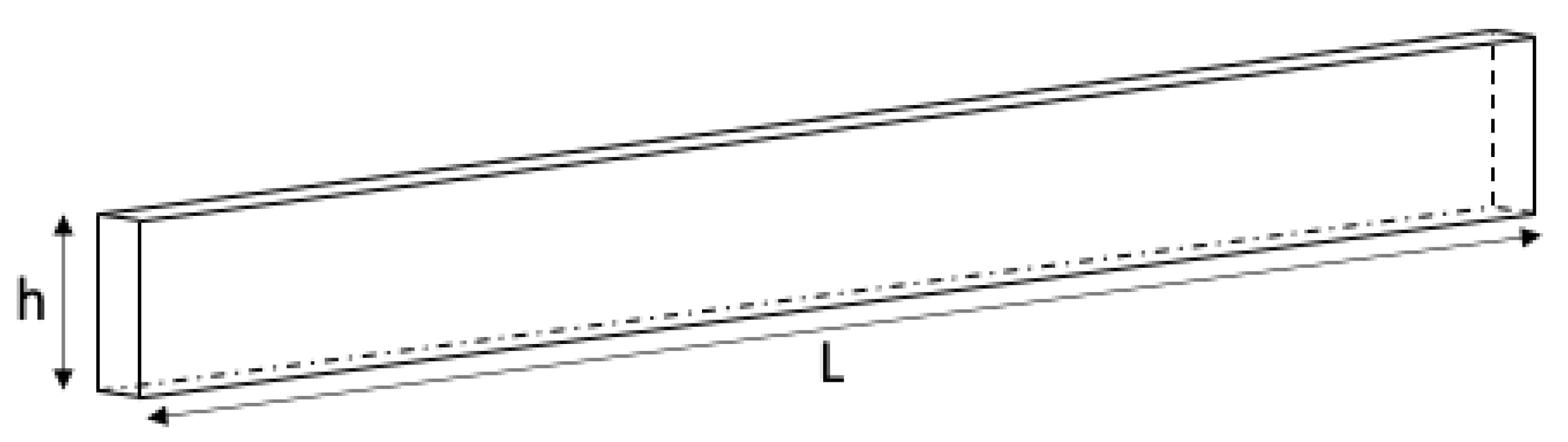
Grid independence was also performed on the 2D domain shown in Figure 1 where the length, L, is $0.1$ $\mathrm{m}$ and the height, h, is $0.005$ $\mathrm{m}$. The parameters of interest in the grid-independence study are the development of the thermal boundary layer and resultant temperature profile throughout the domain, therefore, grid independence was performed by increasing the number of control volumes in the thickness direction, h. The inlet and wall temperatures were fixed at $333.15$ $\mathrm{K}$ and $393.15$ $\mathrm{K}$, respectively. The fiber volume fraction is 50% and the inlet velocity is $0.005$ $\mathrm{m}$/$\mathrm{s}$. A total of five different mesh densities were used; three with uniform grid spacing and two with edge refinement towards the upper and lower walls.

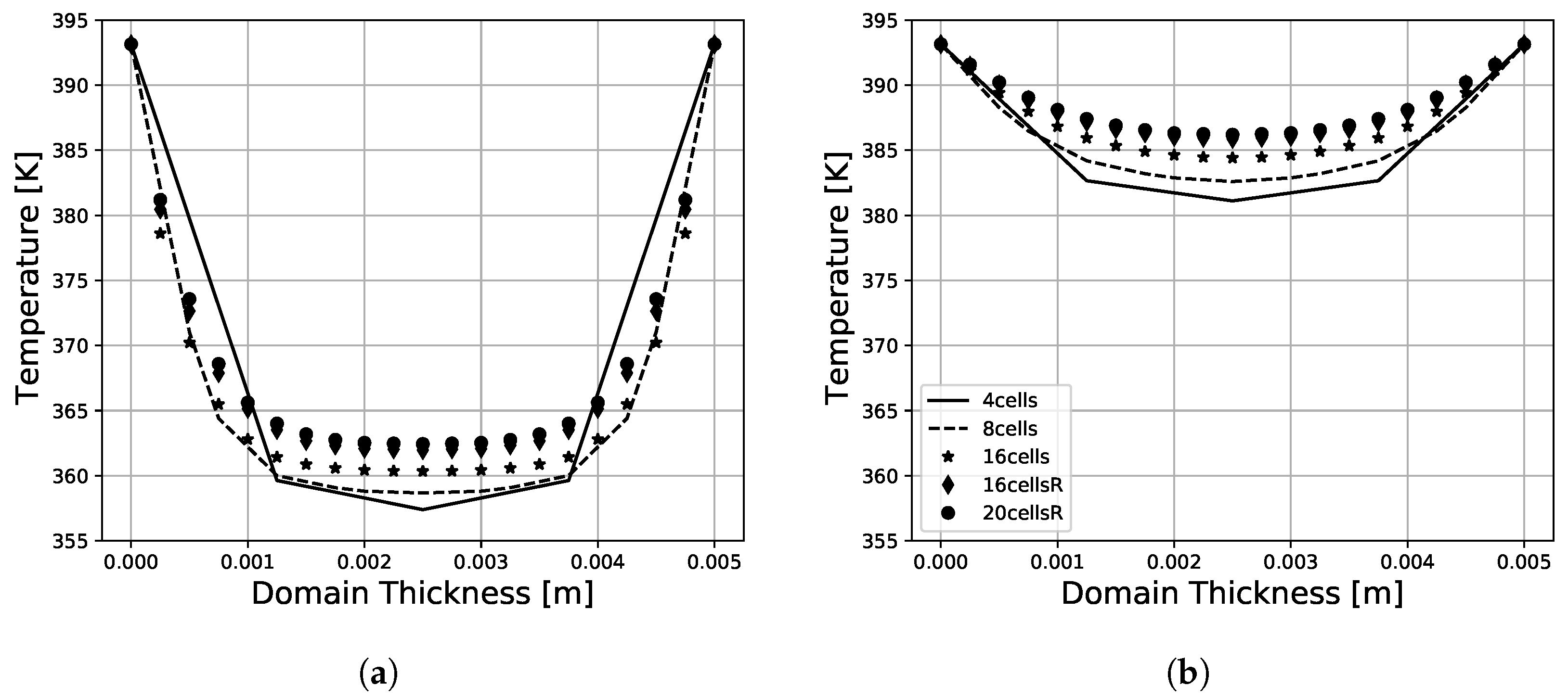
Temperature profiles were extracted at two different locations along the length, 25 $\mathrm{m}$$\mathrm{m}$ and 75 $\mathrm{m}$$\mathrm{m}$, and are shown in Figure 2a,b, respectively. At 25 mm, it is seen that the minimum temperature in the domain is consistent among the 5 grids, however, the temperature gradient at the wall varies dramatically with increased grid resolution. Correctly predicting this temperature gradient is critical as it dictates the heat flux into the domain. This is observed in the temperature profiles at 75 $\mathrm{m}$$\mathrm{m}$ where there is a 30 $\mathrm{K}$ temperature discrepancy between the domains with 4 and 20 cells in the thickness direction. Grid independence was calculated based on the minimum temperature at 75 $\mathrm{m}$$\mathrm{m}$. Using the grid convergence index described by Celik et al. [35], it was found that with 20 cells in the thickness direction with edge refinement, the grid was converged to less than 1%.

3.2. Temporal Resolution Study

The dependency of the source term, in both the thermal equilibrium and thermal LTNE energy models, on the simulation time step requires a time-step independence study be performed to ensure that the predicted temperature rise from the models is correct. This is achieved by modelling the curing stage and reducing the complexity of the simulation to 1D whereby zeroGradient boundary conditions are applied to all faces in the domain, shown in Figure 1. This allows the numerically predicted temperature rise to be directly compared to the analytical temperature rise using

$$ϵq=\widetilde{C_p}(T_2-T_1)$$

(23)

where $ϵ$ is the porosity, q is the total specific heat released, $\widetilde{C_p}$ is the effective specific heat and $T_1$ and $T_2$ are the initial and final mixture temperatures, respectively. For this verification test, the domain was assumed to be completely saturated with resin (i.e., $\alpha$ = 1), with a uniform cure degree of $0\%$. The simulation then ran until a maximum cure degree of $60\%$ was achieved, at which point the analytical and numerical temperature rise were compared.

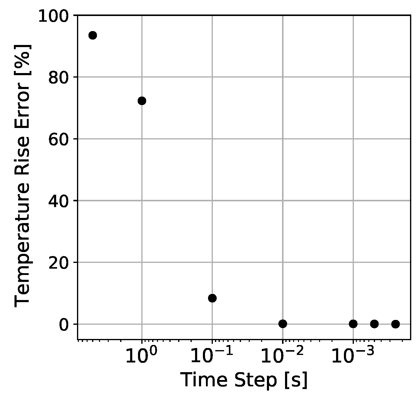
The time-step range used in this study was 0.0025 $\mathrm{s}$–5 $\mathrm{s}$ to predict the resulting temperature rise error between the analytical determined and numerically predicted temperature. The results are given in Figure 3, which shows that the required time step to ensure numerical accuracy is $0.01$ $\mathrm{s}$. With this time step, it was found that there was a temperature rise error of 0.09%. This result verifies that the heat release model used in the thermal equilibrium and LTNE energy model are correctly predicting the heat release and resulting temperature rise.

3.3. Non-Dimensional Analysis

The increased accuracy of the LTNE energy model comes at the cost of longer computational time due to the additional energy equation being solved for the solid phase as well as the coupling required between fluid and solid energy equations. Given the number of variations on the RTM process, the balance between increased accuracy and computational requirements may not be inherently clear. To this end, a study was performed to determine when the LTNE energy model is necessary to provide accurate predictions.

To be able to accurately compare the predicted temperature development during infiltration, non-dimensional groups that contain the parameters that contribute most to the temperature evolution are determined. For RTM, these parameters are: (i) the permeability of the fabric, (ii) the thickness of the part, and (iii) the velocity of the resin being injected. These parameters can be used to form a Darcy number, $Da$, and a Peclet number, $Pe$. The Darcy number is given as

$$Da=\frac{\mathit{K}}{h^2}$$

(24)

where h is the thickness of the domain, and $Pe$ is given as

$$Pe=\frac{vh}{\alpha }$$

(25)

where $\alpha$ is the thermal diffusivity, defined as

$$\alpha =\frac{k}{\rho C_p}.$$

(26)

The influence of $Da$ and $Pe$ are observed in variations of the fluid temperature, both when compared to the injection and mold temperature, as well as the solid temperature. These differences are captured using the non-dimensionalized fluid temperature, ${\theta }_f$, defined as

$${\theta }_f=\frac{T_f-T_{wall}}{T_{inj}-T_{wall}}$$

(27)

where $T_f$ is the local fluid temperature, $T_{wall}$ is the prescribed wall or mold temperature, and $T_{inj}$ in the resin injection temperature. The fluid–solid temperature difference will be captured using the local thermal non-equilibrium parameter, $LTNE$, given as

$$LTNE=T_f-T_s$$

(28)

where $T_s$ is the local solid temperature. A range of Darcy numbers based on the part thickness, h, $Da\in (4.2\mathrm{e}-5,9.5\mathrm{e}-5,3.8\mathrm{e}-4,\mathrm{e}-3)$, and Peclet numbers numbers based on the inlet velocity, v, were varied from $Pe\in (400,4000)$. These values were chosen to provide a comparison over a wide range of part thicknesses and injection velocities to understand the effect of using an LTNE model on RTM and HP-RTM manufacturing methods. Each $Da$ and $Pe$ number case is also run for two conductivity ratios (i.e., $k_s/k_f$ of 0.2 and 125) which correspond to the use of either glass or carbon fibers within the mold. The boundary conditions used for all subsequent simulations are given in

Table 1. Boundary conditions used for non-dimensional analysis cases.

Location	Field Type	Value
inlet	Velocity	fixedValue
	$cure$	0%
	$T_f$	$363.15\mathrm{K}$
	$T_s$	$393.15\mathrm{K}$
upperMold	Velocity	noSlip
	$T_f$	$393.15\mathrm{K}$
	$T_s$	$393.15\mathrm{K}$
lowerMold	Velocity	noSlip
	$T_f$	$393.15\mathrm{K}$
	$T_s$	$393.15\mathrm{K}$
wall	Velocity	noSlip
	$T_f$	$393.15\mathrm{K}$
	$T_s$	$393.15\mathrm{K}$
symmetry	Velocity	symmetry
	$T_f$
	$T_s$

.

3.4. Temperature Distribution and Development

The non-dimensional temperature (${\theta }_f$) and LTNE profiles are plotted as a function of the non-dimensional channel height in Figure 4. Since the profiles are all symmetric, each figure shows data contrasting two conductivity ratios; the left and right sides of each plot show data for conductivity ratios of 0.2 (black symbols) and 125 (grey symbols), respectively, for the same $Da$ and channel location. Furthermore, the plots in Figure 4 are arranged such that the first and second columns show ${\theta }_f$ at locations of 25% and 75%, respectively, and the third and fourth columns show the LTNE at locations of 25% and 75%, respectively. Each row corresponds to a specific $Da$ number, as denoted by the symbols in the legend.

Considering first the influence of $Da$ number, the results show that as $Da$ decreases, use of the LTNE model bears diminishing returns. The cases where $Da\in (9.5\times {10}^{-5},4.2\times {10}^{-5})$ for a $Pe\in (400,2000)$ and a $k_s/k_f=0.2$, show the local temperature difference for the fluid and solids phases is less than 5 $\mathrm{K}$. In these cases, the low conductivities of the fluid and fibers reduce the influence of the fixedValue boundary condition at the mold wall. This, therefore, allows the resin to cool the fiber phase and bring them closer to thermal equilibrium. This is highlighted in Figure 4m–p, for a $Pe=400$, where there is no discernible difference between the fluid and solid temperatures throughout the domain. This suggests that an equilibrium energy model could be used to model this case as the fluid and solid phases are in local equilibrium throughout infiltration. However, when considering a $k_s/k_f=125$, the conductivity ratio has a significant effect on the LTNE, especially at the start of infiltration. For all Darcy numbers considered, it was found that the higher conductivity ratio increased the resin temperature significantly faster than the lower conductivity ratio cases. The end result of this rapid warming is seen in the ${\theta }_f$ profiles at $x/L=0.75$, where for each $Pe$ the resin is closer to the mold temperature. This suggests that for cases where a $Pe>1000$ an LTNE energy model is needed. An additional consideration when performing a comparable case is the influence that this rapid increase in fluid temperature has on both the cure and viscosity development during infiltration. Given the increasingly large number of resins that can be used for RTM, this temperature rise could potentially result in premature curing or vitrification of the resin.

As $Da$ increases, an increase is observed in both the local ${\theta }_f$ and LTNE throughout the thickness of the part, even for the cases where $Pe=400$. Although in these cases the $Da$ was varied based on the height of the part, the increase in $Da$ is also analogous to a reduction in fiber volume fraction (considering the high dependence the permeability of the fabric has on fiber volume fraction). This in turn reduces the influence of the fiber phase on the fluid temperature, which is observed in Figure 4a–d, where for each $Pe$ the fluid temperature is closer to the mold temperature. The solid phase still contributes to the increase in fluid temperature, however, due to the transient nature of the flow, this influence is not as substantial as the mold temperature. The solid phase influence on the fluid temperature is also affected by the conductivity ratio. The higher the conductivity of the fibers, the less influence the fluid phase has on the temperature of the solid phase. This is due to the rapid conduction from the mold to the fibers throughout the domain, maintaining more of the fiber phase at the mold temperature. The result is an increase in the local fluid temperature due to the increased heat transfer from the solid phase to the fluid phase. This effect is highlighted in the LTNE plots in Figure 4, specifically at $x/L=0.25$, which show increased LTNE between the fluid and solid phases for the higher fiber conductivity. Although this result is not intuitive given that the higher solid temperature would result in increased heat transfer from the fibers to the resin, the conductivity from the mold wall to the fiber phase maintains the fibers at a higher temperature when compared to the lower conductivity fibers.

The $Pe$ number also has a significant effect on the local fluid temperature during mold filling due to its direct connection with filling time. Increasing the $Pe$ number reduces the filling time and consistently results in larger differences between the fluid, solid and mold temperatures. Increases in $Pe$ number also inherently increase the convective heat transfer between the solid and fluid phases, but this increase in heat transfer does not always lead to increases in fluid temperature because of the increased fluid velocity. The reduction in filling time from a $Pe$ number of 400 to 4000 is 10 times (for a $Da=1\times {10}^{-3}$). This in turn reduces the time that the increased convection heat transfer has to increase the resin temperature. The $Da$ number also has an effect on the influence of the $Pe$ number. As previously mentioned, reducing the $Da$ number results in an increased effect of the mold temperature on the fluid temperature in the center of the domain. Coupling these two influences together, it is observed that for a $Pe>1000$ number, when the $Da$ number is reduced, the resulting fluid temperature profile both near the inlet and near end of the domain is closer to the mold temperature than the injection temperature.

These generic results highlight the utility of the LTNE energy model for RTM and HP-RTM processes. It is also important to note that additional attention needs to be directed at cases with large infiltration times since there exists the potential for premature curing of some resins. Furthermore, a longer infiltration time implies a longer cycle time to produce parts.

3.5. Fluid Property Development

Capturing the temperature development of the flow front also has implications on the predicted development of other fluid properties. Two critical properties, the fluid viscosity and cure degree, are heavily influenced by the history of the fluid temperature as it infiltrates the mold. This effect is captured by comparing the fluid property development for the $Da=1\times {10}^{-3}$ and $Pe=4000$ case with a $k_s/k_f=125$, using the current LTNE and thermal equilibrium energy models. The coefficient values for the Kamal–Malkin reaction kinetic model, DiBeneditto glass transition temperature model, and Castro–Macosko viscosity model are given in

Table 2. Parameter values used for the Kamal–Malkin kinetic model.

Model Parameter	Value
$A_1$	3,862,141.7
$A_2$	105,920,589,010.0
$E_1$	62,877.7
$E_2$	321,915.1
m	1.571
n	1.63
R	8.314

,

Table 3. Parameter values used for the DiBeneditto glass transition temperature model.

Model Parameter	Value
$T_{g,0}$	243.0
$T_{g,\infty }$	406.09
$\lambda$	0.390

and

Table 4. Parameter values used for the Castro–Macosko viscosity model.

Model Parameter	Value
$C_1$	3.91
$C_2$	$2.12\times {10}^{-13}$
B	$1.414\times {10}^{-12}$
$T_b$	$8.489\times {10}^3$
R	8.314
$c_g$	0.72

, respectively.

Figure 5 compares the fluid viscosity profile at two different locations within the domain, $x/L=0.25$ and $x/L=0.75$. It can be readily observed that the fluid viscosity near the mold walls is lower for the equilibrium model. This is due to the weighting factors ($w_f$ and $w_s$) used to calculate the local fluid–solid mixture properties. Equations (12) and (13) show that the weighting factors are determined based on the density of the two phases. Considering that the density of fibers is nearly double that of the resin phase and coupled with the high conductivity ratio between the fluid and solid phases, it is expected that the model would predict a rapid increase in fluid temperature from the injection temperature to the mold temperature. This is captured in Figure 5a where it is shown that the viscosity of the fluid is lower near the wall when compared to the LTNE energy model. The effect of the rapid increase in temperature is further shown in Figure 5b, where the viscosity of fluid throughout the domain cross-section is substantially less for the equilibrium model than the LTNE model. In this respect, the LTNE model is also essential for properly predicting the pressures required for mold filling and the flow distribution since both are strongly affected by local viscosity.

The effect of the energy model on the cure degree development is shown in Figure 6. As with the fluid viscosity, there is a small discrepancy in the predicted cure degree at a $x/L=0.25$, where the cure degree is higher at the walls in the equilibrium model due to the higher predicted temperature. At $x/L=0.75$ this difference increases substantially, where the non-equilibrium model predicts the average cure degree to be 0.5% and the equilibrium model predicts 1.9%. The implications of this difference are significant. First, the source term added to the fluid temperature equation, Equation (16), will predict a larger heat release at the end of infiltration for the equilibrium energy model. This can lead to local rises in temperature in the domain, which can result in the prediction of premature curing. Furthermore, if the curing stage is to be simulated, this result would incorrectly predict a shorter curing time, which can have a significant impact on the material properties of the final parts. Secondly, in both Figure 5 and Figure 6, it is observed that at $x/L=0.75$ there is a transition in the viscosity and cure degree for the equilibrium case adjacent to the mold walls. The cause of this is the resin being in the domain at the mold temperature. There is an initial reduction in the resin viscosity near the mold walls as it warms, as seen in Figure 5a for both cases, but given the higher overall temperature in the domain for the equilibrium case, the resin reaches the mold temperature considerably faster. At $x/L=0.75$ the resin viscosity is substantially lower for the equilibrium case but there are signs of premature curing near the walls given the local increase in fluid viscosity. Considering the cure profile in Figure 6, this increase in viscosity at the walls is due to a sharp increase in the local cure degree. Given the viscosity’s dependency on the cure degree, this result is expected.

The implications of these results on predicting mold filling behaviour and cure degree development in RTM components are significant; the most significant being the resultant flow front predicted from the thermal equilibrium model. The local decrease in viscosity near the mold walls will result in a higher fluid velocity due its inclusion in Darcy’s law. This advancing front near the walls can lead to predictions of void formation in the final part, especially for parts with a high $Da$ or with multiple inlets resulting in multiple flow fronts meeting. There is also the potential for the prediction of premature curing of the resin at the mold walls. This can result in the prediction of local hot spots, depending on the resin and fiber properties, as well as inaccurate prediction of the required time for the curing stage. Finally, it was found that the computational cost of using an LTNE model was on the same order of magnitude as the thermal equilibrium. This is due to time scale of the heat transfer occurring when compared to the time scale of the fluid movement. The VOF method used to track the infiltration of the resin required a substantially lower time step than the energy model. This is a significant finding as it means the added computational cost of the LTNE model is reasonable given the increased accuracy when predicting the temperature development.

3.6. Complex Floor Geometry

Simulation of resin infiltration in a complex floor geometry is presented as a final case to further demonstrate the efficacy of the LTNE model compared to isothermal energy modelling and to thermal equilibrium modelling. The complex mold geometry is shown in Figure 7a. The computational mesh is shown in Figure 7b, where the domain has been discretized into 988,000 hexahedral elements. Meshing was performed using the results from the grid independence test in Section 3.1 where four cells per $\mathrm{m}$$\mathrm{m}$ of part thickness, with edge refinement towards the upper and lower surfaces, was used. The boundary conditions, as well as the coefficients for the Kamal–Malkin reaction kinetics and Castro–Macosko viscosity models, are found in Table 1, Table 2 and Table 4, respectively. The fiber volume fraction was set to a uniform value of 50% and the fiber orientation was assigned using a simple geometric approach that established in-plane and cross-plane components based on the local position of the upper and lower mold faces. While more sophisticated approaches are available for determining local fiber orientation, for the purpose of demonstrating the LTNE model, a simple approach was deemed suitable.

3.6.1. Infiltration

The progress of the cure degree during infiltration for each of the four cases is shown in Figure 8. Columns one and two in Figure 8 consider the assumption of isothermal mold filling. These results also highlight the significant impact of operating temperature on the cure degree development during mold filling. As the operating temperature increases, the maximum cure degree in the domain is shown to also increase. This is further shown in

Table 5. Minimum and maximum cure degree values in the domain after infiltration for each energy modelling approach.

Energy Modelling Approach	Maximum Cure Degree	Maximum Cure Rate
Isothermal 363 $\mathrm{K}$	0.96%	$0.3$%/$\mathrm{s}$
Isothermal 393 $\mathrm{K}$	4.6%	$1.7$%/$\mathrm{s}$
Thermal Equilibrium	4.5%	$1.7$%/$\mathrm{s}$
Thermal Non-Equilibrium	3.5%	$1.6$%/$\mathrm{s}$

, where a 3.6% difference in the maximum cure degree is shown between the two isothermal simulations. As expected, the areas of highest cure degree are at the edges of the component, as this corresponds to the resin that has been in the domain for the longest period of time. A major implication of this, in particular for the isothermal 363 $\mathrm{K}$ simulations, is an incorrect prediction of the required curing time needed to fully cure the resin. This will be discussed in further detail in Section 3.6.2.

The most interesting results are evident when comparing the cure degree distribution for the equilibrium and LTNE energy models. Considering first the equilibrium energy model, it is observed that the maximum cure degree does not differ significantly compared to the isothermal 393 $\mathrm{K}$ case (4.5% and 4.6%, respectively, as shown in Table 5). This is also seen when comparing the cure degree distributions during infiltration. The cure degree contours shown in Figure 8 are nearly identical at all points during infiltration, with the only noticeable difference being at the bottom left hand edge of the part. In this region, the thermal equilibrium model is showing a lower cure degree compared to the isothermal 393 $\mathrm{K}$ case. The similarity in cure distribution is explained by the formulation used to determine the average material properties used in the equilibrium energy model (Equations (9)–(11)), in particular Equation (11), used to calculate the mixture conductivity. For these simulations the conductivity ratio between the solid and fluid phases ($k_s/k_f$) is 125. The high fiber conductivity forces a rapid increase from the injection temperature (363 $\mathrm{K}$) to the mold temperature (393 $\mathrm{K}$) immediately after the resin is injected. The infiltration then proceeds as though done isothermally at the prescribed mold temperature. As mentioned previously, this phenomenon is highly dependent on the thermophysical properties of the resin and fibers. For a lower conductivity ratio (i.e., using glass fibers) there would be a large discrepancy between the maximum cure degree with the domain when compared to the isothermal 393 $\mathrm{K}$, as it would take longer for temperature to rise to the mold temperature in the domain.

This result is consistent with the predicted cure degree development for this complex geometry, where the Peclet number is 6780. Recall from Section 3.3 that for almost all cases where the Peclet number is greater than 1000 (with a conductivity ratio of 125), an LTNE model is needed to accurately capture the development of the fluid temperature during infiltration. The results predict a longer period of time where the cool injected resin warms to the mold temperature, when compared to the equilibrium model, as shown by the large region of less cured resin in center of the complex part. This suggests that the resin and fibers are not in local thermal equilibrium. The areas where the resin has warmed to the mold temperature and has been in the domain the longest are at the corners, which carry the highest resin cure degree of 3.5%. The lower predicted maximum cure degree means there is overall less variation in the cure degree distribution, when compared to the equilibrium energy model. The result is a more even development of the cure degree during the cure stage, which is discussed further in Section 3.6.2.

3.6.2. Curing

Results of the cure degree and temperature distribution at the end of the infiltration stage were used as the initial conditions for curing simulations. The resin was allowed to cure for 180 $\mathrm{s}$, using the four energy modelling approaches, and the resulting cure degree and cure rate at 10 $\mathrm{s}$ are shown in Figure 9 and Figure 10, respectively. Due to the large change in cure degree during the curing stage, the cure degree contour plot in Figure 9 only contains data at 10 $\mathrm{s}$. Were a longer time range considered, the fine detail of the cure degree distribution would be lost. To address this, the cure degree range for each energy modelling approach (at times 10 $\mathrm{s}$, 100 $\mathrm{s}$, and 180 $\mathrm{s}$) are shown in

Table 6. Cure degree distribution ranges for each case during the curing stage.

Energy Modelling Approach	Cure Degree Range (Min–Max)
	10 s	100 s	180 s
Isothermal 363 $\mathrm{K}$	3.4–4.3%	26.9–27.5%	40.9–41.3%
Isothermal 393 $\mathrm{K}$	14.9–18.5%	68.5–69.2%	81.8–82.1%
Thermal Equilibrium	14.5–18.4%	68.4–69.2%	81.8–82.1%
Thermal Non-Equilibrium	12.5–17.6%	68.0–69.0%	81.6–82.0%

. In the case of Figure 10, the isothermal 363 $\mathrm{K}$ case had a significantly lower cure rate, which if included would have again resulted in the loss of the fine detail in the cure rate distribution.

Columns one and two in Figure 9 show the cases of isothermal curing. The results further highlight the dependence of the cure degree development on the operating temperature. At the start of the curing stage there is a 12% difference in the average cure degree between the two isothermal cases. At the end, however, the discrepancy in average cure degree has grown to 41%, shown in Table 6. This is due to the lower operational temperature in the isothermal 363 $\mathrm{K}$ case which restricts the cure rate during the course of the curing stage. It should be noted that an operating temperature of 363 $\mathrm{K}$ is unlikely to be used in practice for this case given the additional time needed to cure the component, however, it reinforces the importance of optimizing the operating temperature through simulation and for manufacturing of CoFRP components.

Consistent with the infiltration stage, the cure degree distribution for the isothermal 393 $\mathrm{K}$ and equilibrium model show nearly identical development during curing. This result is further highlighted in Table 6 where at each recorded time the minimum and maximum cure degree varies at most by 0.4% and in the case of 180 $\mathrm{s}$ it is shown that the cure degree ranges are identical. Again, this is due to the resin rapidly increasing from the injection temperature to the mold temperature when using the equilibrium model, resulting in the model behaving as though the process was done isothermally. An interesting outcome is the similarity in final cure degree distributions predicted by the isothermal 393 $\mathrm{K}$, equilibrium, and LTNE models at 180 $\mathrm{s}$. To fully understand this outcome, consideration first needs to be made with regard to the type of curing being performed. Bernath et al. [31] studied the influence of the type of cure modelling being used (i.e., isothermal versus non-isothermal) and the ability of the reaction kinetics model to capture the resulting cure degree progression as compared to experimental data. Their results showed the cure rate profile for isothermal curing begins with a peak in cure rate which quickly diminishes for the remainder of the cure cycle. For non-isothermal curing, however, there is a noticeable delay in the peak cure rate (the magnitude and time of which are highly dependent on the rate of temperature increase), due to the time needed for the resin to warm. The results of the present study are consistent with the findings of Bernath et al. [31]. For the isothermal 393 $\mathrm{K}$ and equilibrium cases (for which isothermal curing conditions are used) an initial peak in cure rate was observed (highlighted again by the higher cure degree at the beginning of the cure stage), which then quickly diminished during curing. In the case of the LTNE model, which simulates initially non-isothermal curing, the peak cure rate is observed post-infiltration, during the curing stage. This phenomenom is further highlighted in Figure 10, where the LTNE model is showing a cure rate nearly 8% higher throughout the component. The LTNE model then consistently predicts a higher cure rate for the entirety of the simulated cure cycle, resulting in a nearly identical cure degree distribution between the three cases.

A comment needs to be made on the limitation of the Kamal–Malkin kinetic model due to its reduction in accuracy as the glass transition temperature approaches the operating temperature. Were a more sophisticated kinetic model used, it is hypothesized that the LTNE case would predict a final cure degree distribution higher than that found in the isothermal 393 $\mathrm{K}$ and equilibrium models. This is due to the overall higher cure rate still present throughout the cure cycle in the LTNE energy model, as well as the results presented by Bernath et al. [31]. A consistent result seen in their work shows that in the case of isothermal curing, the final cure degree achieved is highly dependent on the operational temperature and is consistently less than 100%; a result not found in non-isothermal curing where the resin maintains the ability to nearly completely cure. A caveat to this, however, is the unknown effect of combining isothermal and non-isothermal curing. This combination is found in the LTNE case, where curing is initially non-isothermal, as the cool injected resin warms to the mold temperature. After 10 $\mathrm{s}$ of curing, the resin reaches the operating temperature of 393 $\mathrm{K}$ and continues the curing cycle isothermally. This likely slowed the overall peak cure rate, however, allowing the model to maintain an overall higher cure rate. An implication of this might be when predicting the final material properties as well as process-induced distortion (PID) [22]. The maximum achievable cure degree has a significant impact on the final material properties and dictates the amount of chemical shrinkage that occurs. Chemical shrinkage influences the build-up of residual stresses leading to PID. This further reinforces the importance of an accurate prediction of the temperature evolution given its influence on the cure development. It also highlights the importance of the reaction kinetic model utilized. As mentioned above, a limitation of the Kamal–Malkin kinetic model is that it always predicts full resin curing despite the operating temperature, which is known to not be the case. For a better understanding of the operating temperature on the maximum possible cure degree as well as the cure degree progress post-vitrification, the more sophisticated Grindling reaction kinetic model could be utilized.

4. Summary

The current study was aimed at studying the complexity viability of an LTNE energy model for obtaining accurate solutions of temperature development in RTM mold-filling simulations. A general LTNE model was implemented into an existing mold-filling code in OpenFOAM. A non-dimensional analysis was then conducted over a range of $Da$ numbers, $Pe$ numbers, and $k_f/k_s$ ratios to show the non-dimensional fluid temperature and local thermal non-equilibrium development, for a wide range of part types and infiltration strategies. Results from the non-dimensional analysis show that for a $Da\in (9.5\times {10}^{-5},4.2\times {10}^{-5})$, $Pe\in (400,1000$) for a $k_s/k_f=0.2$ and a $Pe=400$ for a $k_s/k_f=125$, the approximation of local thermal equilibrium is appropriate. However, for all other case runs it was shown that for an accurate prediction of the resin and solid temperature during mold filling, the use of an LTNE model was required.

To further understand the implications of using a thermal equilibrium model when a non-equilibrium model is required, a comparison case was run where $Da=1\times {10}^{-3}$ and $Pe=4000$ with a $kf/ks=125$ using a equilibrium energy model from the literature and the proposed non-equilibrium model. The result further highlights the importance of using a thermal non-equilibrium model. The predicted resin cure degree for the case using the equilibrium model were substantially higher near the end of the domain due to the rapid increase in temperature throughout the domain. This resulted in a much lower resin viscosity, due to its dependency on the cure degree. The implications of this are an inaccurate prediction of the cure time needed in the curing stage, as well as the potential for a void to form if multiple flow fronts meet given the advancement in the resin front near the mold walls. It was also found that the additional computational cost was minimal, implying that the thermal non-equilibrium model is able to be used effectively in all RTM infiltration modelling.

A complex floor geometry was then used to evaluate three energy modelling approaches; isothermal mold filling (at operating temperatures of 363 $\mathrm{K}$ and 393 $\mathrm{K}$), thermal equilibrium, and LTNE energy modelling. Both the infiltration and curing stages were modelled using the four different energy modelling approaches. The isothermal 363 $\mathrm{K}$ cases highlighted the effect of the operating temperature on the final cure degree, where a 3.6% difference in the maximum cure degree was found between the two isothermal mold-filling simulations. When considering the equilibrium energy model, it was found that the cure degree distribution was nearly identical to that predicted by the isothermal 393 $\mathrm{K}$ simulation. This was due to the weighting factors used to calculate the effective thermophysical properties employed in the energy transport equation. The most notable outcome was that of the LTNE energy model. The LTNE predicted a lower maximum cure degree as well as a larger area of less cured resin within the domain. This result highlights the increased accuracy in the predicted temperature development and resulting cure degree as the results show the fibers and resin are not in thermal equilibrium. The curing stage highlighted the importance of which energy model was used for the infiltration stage. In the case of the isothermal 363 $\mathrm{K}$, isothermal 393 $\mathrm{K}$, and equilibrium energy modelling, it was shown that curing occurred isothermally. The result of an initial peak in the cure rate during infiltration which quickly diminishes at the beginning of the curing stage. In the case of LTNE energy modelling, the cure degree development follows a more complex path, where it initially develops non-isothermally during infiltration and at the beginning of the curing stage. After 10 $\mathrm{s}$ of curing the resin has reached the prescribed mold temperature and then continues its curing under isothermal conditions. The effect of this has implications when considering the predicted material properties and PID from each case, given their dependency on the final cure degree. Moreover, it highlights the importance of the reaction kinetic model used. The selected Kamal–Malkin kinetic model predicts that resin would cure fully despite the operating temperature. Using a more complex kinetic model, such as the Grindling model, would provide better insights into the true final cure degree and cure degree development given the models ability to predict vitrification. Finally, it was also found that the use of an adaptive time step dependent on the current maximum cure rate and minimum cure degree, in conjunction with the LTNE model dramatically reduced the computational time of the curing stage. This further increases the applicability of an LTNE energy model for HP-RTM infiltration and curing simulation.