
Derivation and Validation of Linear Elastic Orthotropic Material Properties for Short Fibre Reinforced FLM Parts


Engineering Design, Friedrich-Alexander-Universität Erlangen-Nürnberg, 91058 Erlangen, Germany
*
Author to whom correspondence should be addressed.
J. Compos. Sci. 2022, 6(4), 101; https://doi.org/10.3390/jcs6040101
Submission received: 10 February 2022
/
Revised: 3 March 2022
/
Accepted: 4 March 2022
/
Published: 22 March 2022
(This article belongs to the Special Issue Characterization and Modelling of Composites, Volume II)
Abstract
:Additively manufactured parts play an increasingly important role in structural applications. Fused Layer Modeling (FLM) has gained popularity due to its cost-efficiency and broad choice of materials, among them, short fibre reinforced filaments with high specific stiffness and strength. To design functional FLM parts, adequate material models for simulations are crucial, as these allow for reliable simulation within virtual product development. In this contribution, a new approach to derive FLM material models for short fibre reinforced parts is presented; it is based on simultaneous fitting of the nine orthotropic constants of a linear elastic material model using six specifically conceived tensile specimen geometries with varying build direction and different extrusion path patterns. The approach is applied to a 15 wt.% short carbon-fibre reinforced PETG filament with own experiments, conducted on a Zwick HTM 5020 servo-hydraulic high-speed testing machine. For validation, the displacement behavior of a geometrically more intricate demonstrator part, printed upright, under bending is predicted using simulation and compared to experimental data. The workflow proves stable and functional in calibration and validation. Open research questions are outlined.
1. Introduction
1.1. Motivation
Additively manufactured parts for structural applications have gained importance in recent years in both research and industrial applications, shifting from models and prototypes towards end use parts and products [1,2]. This development is accompanied by the need for suitable processes and materials as well as reliable simulation models, as the Design for Additive Manufacturing (DfAM) pre-process is largely based on virtual product development [2,3]. Through virtual product development, fulfilment of requirements and an efficient development process can be ensured preceding the physical product [4].
In terms of material choice, especially fibre reinforced polymers (FRP) have gained importance due to their favourable specific stiffness and strength and wide range of applications [5,6,7,8,9,10,11,12] while their material costs in AM can be lower than for metal AM materials, although overall cost including machining and labour has to be considered [13]. Concerning the choice of FRP, Such et al. [14] cite a patent [15] which considers short FRP a “sweet spot” between mechanical performance (best: endless fibre) and manufacturability (best: no fibre at all). Both short fibre and endless fibre FRP can be manufactured using the Fused Layer Modeling (FLM) process, which allows for higher design freedom when compared to other FRP-capable processes such as Laminated Object Manufacturing (LOM; limited fibre orientation capabilities) or stereolithography (SLA; very limited fibre orientation capabilities and low fibre weight fraction, only with short fibre FRP) [16]; moreover, correlating with low material costs, FLM is commonly more readily available when compared to other AM processes such as Laser Sintering (LS). For these cost-efficiency, mechanical property and design freedom reasons, this contribution focuses on the derivation and application of material models for short fibre FRP FLM-printed structural parts. To introduce the principle of FLM, the hot-end of a FLM printer and its schematic illustration is given in Figure 1a. Extrusion beads of heated thermoplastic filament are laid side-by-side on a printing platform, initially; and on top of preceding layers, subsequently. In-plane orientation of beads is divided into contours (outer border walls) and infill (inner structure between border walls). Overhangs are upheld by support structures which are removed after printing.
1.2. State of the Art and Objectives
For the effective design of structural parts, several attempts have been made to enable simulation-based design, which predominantly address the mechanical characterization of standard test specimens, mostly tensile testing, to derive a certain set of material parameters. The following section provides an overview of existing approaches.
There has been broad research in the mechanical characterization of FLM test specimen which to a large extent focused on unreinforced polymers, mostly acrylonitrile butadiene styrene (ABS). Montero, Ahn et al. [17] in 2001 scrutinized ABS tensile specimen with various geometries for material characterization and compared these FLM results with injection-molded samples. FLM samples yielded 65–72% of the strength of injection-molded parts. Furthermore, from testing experience, build rules for FLM parts were derived: (1) tensile loads should be carried axially along the “fibres”; (2) radii shall be built using contours (instead of lines/grid rasters); (3) negative air gap (bead overlap), Figure 1b, increases strength and stiffness (air gap larger than −0.002 inches, i.e., 0.0508 mm); (4) “Shear strength between layers is greater than shear strength between roads” [17]; and (5) bead width and temperature do not affect strength, but have to be considered concerning build time, surface quality and wall thickness. In the following year 2002, Ahn, Montero et al. [18] published a contribution concerning the anisotropic material properties of FLM ABS. The air gap, road width, model temperature, ABS color and raster orientation were varied and their influence on mechanical properties (tensile and compressive strength) studied; this led to a complement to their building rules: (6) Tensile loaded area tends to fail easier than compression loaded area (later tests indeed showed a tendency towards that, however, there is variation in results [19,20,21]). A large impact of FLM process parameters on mechanical properties was also found by Pei et al. [22] as well as Ning et al. [10], largely confirming Ahn and Montero’s build rules, though Ning et al. additionally point out that there is a sweet spot in printing temperature: a temperature too low provokes weak layer interbonding, while a temperature that is too high implicates more pores, decreasing tensile properties. Li et al. [23] proposed a geometrical ellipse-based theoretical material model for FLM parts, which was successfully validated using tensile tests (3.1 to 7.1% of deviation between material model and experiment). This model accounts for voids produced by the FLM process, Figure 1b, and is, in turn, based on a Stratasys® ABS P400 material model by Matas et al. [24]. Bellini et al. [25] proposed a method to derive orthotropic material models for FLM parts with pre-defined infill rasters of [0° 90° +45° −45°] and Delaunay-Triangulation based “domain decomposition” infill. This method (which will be adapted and altered later in this contribution) is based on different build-up and infill orientations in six specimen geometries to derive the nine orthotropic material constants. Domingo-Espin et al. [26] also used Bellini’s orientation for a [+45° −45°] infill and validated the method successfully with a hook-like geometry made of polycarbonate (PC). The authors pointed out, however, that the quality of fit of the orthotropic model depends on build orientation and even proposed an isotropic material model for certain cases. Rodríguez et al. [27] proposed a unit-cell based mesoscale method to model FLM-printed ABS and validated their model with less than 10% deviation from experiment. Lee et al. [28] also used ABS to compare FLM, 3D printing (ink jet based) and “nano composite deposition system” (mechanical micro machining included) concerning raster orientation, air gap, bead width, color, and model temperature with focus on compression strength under different build directions (axial and transverse). Compressive strength for FLM was found to be 11.6% higher for axially than for transversely printed specimen. Other, more recent research on unreinforced FLM specimen encompasses Cantrell et al. [29], who included digital image correlation (DIC) in their tensile testing of different infill lay-ups ([+45 −45], [+30 −60] and [0 90]) of FLM ABS specimen. It was found that there is little effect of these stacking sequences on Young’s modulus and Poisson’s ratio; however, shear modulus and shear yield strength were largely affected with variation between results ranging up to 33%. Specimen made of PC behaved similarly; specimen printed upright (tension direction orthogonal to layers), on-edge (flat, but flipped 90° along the longest axis) and flat (tension direction parallel to layers) produced variations of similar magnitude [29]. A Finite Element (FE)-mesostructural model for ABS P400 was conceived and applied by Somireddy et al. [30]. The positive impact of a negative air gap was confirmed therein (“tightly packed”) and a Classical Laminate Theory (CLT)-model was derived to be applied on a 2D FE model of a component. Sheth et al. used a representative volume cell simulation approach with 4 by 4 roads (extrusion beads) and tested this model under varying angles from 0° in steps of 15° to 90°, which showed very good accordance.
Addressing short carbon-fibre reinforced ABS with varying fibre weight percentage (10, 20, 30 and 40 wt.%), Tekinalp et al. [31] found that there is up to 91.5% alignment of fibres in printing direction which leads to significant tensile strength and stiffness increases against unreinforced specimen (+115% and +700%, respectively). The authors also reported nozzle clogging above 30 wt.% fibre content and intensely scrutinized the effect of short fibre reinforcement on voids in and between beads; within beads, voids increased, between beads, voids decreased. These benefits of using FRP within the FLM process sparked interest and further research: Duty et al. [32] scrutinized Big Area Additive Manufacturing (BAAM, nozzle diameter 2.5–7.6 mm instead of the more commonly used 0.2–0.8 mm in FLM) with 13 wt.% short carbon fibre reinforced ABS; anisotropy, stiffness and strength were again increased significantly when compared to unreinforced polymers. A comprehensive overview of various fibre-matrix combinations with different fibre weight fractions was given by Brenken et al. [7]. Mostly, axial to transverse (plane, i.e., within printer platform) stiffness and strength are listed, except for interlayer stiffness and strength by Love et al. [33] For completeness, it is stated that further reviews on 3D printing of FRP have been written by Kabir et al. [11] and Parandoush et al. [16].
To conclude, it can be stated that current specimen-based research largely focuses on comparison between axial and transverse tensile properties (largely within the printer platform plane) or the transfer of specifically built specimen properties (e.g., individual lay-ups in infill) to rather geometrically limited FLM parts. Other approaches include mesoscale models, whose applicability to more complicated geometries and infill patterns, which exploit the large DfAM design freedom, is yet to be shown; and/or 2D models, which may be questionable in case of large through-thickness stresses. A more general approach for deriving material models and transferring these to arbitrary geometries seems necessary to enhance practical applicability and flexibility.
1.3. Objectives and Novelty of This Contribution
This contribution therefore intends to meet the following objectives: (a) Provide a systematic approach to FLM FRP material characterization, which is also transferable to more complicated part geometries, including calibration and validation; (b) Simultaneous fitting of an orthotropic material model (nine constants with moduli and Poisson’s ratios) for arbitrary lay-ups in infill instead of pre-defined infills and (c) scrutiny of the fitting by comparison of orthotropic material model results, which are obtained from calibration within a certain range of error to the experiments, during validation to analyse the effectivity of the method.
The novelty of the work is, firstly, that the z-direction of the printed layer structure is also to be investigated in detail. Secondly, the consideration of component experiments for the validation of the material models is a particular feature of this research. Multiaxial stress states and orthotropic properties are considered during validation. Such investigations have rarely been published before, but promise to offer a great value to enhance the practical applicability of the derived material models.
2. Materials and Methods
Figure 2 presents the overall methodology of this contribution, which consists of four steps: specimen concept and printing (1), experiments (2), fitting of the orthotropic material model (3) and validation simulation/experiment (4).
In the first step, specimens are conceived, which are intended to reflect the orthotropic constants, such as a longitudinally printed 0° tension rod for Young’s modulus parallel to the extrusion beads in axial direction. With these, calibration experiments are conducted (2) which yield force, displacement, stress and strain results. These results, in turn, are used to fit the orthotropic material model parameters of the specimens’ FE simulation models simultaneously for all geometries/infill patterns (3). The orthotropic material model is then applied for validation of the results using a different geometry (“XX-rib”): an orthotropic simulation model fully depicting internal extrusion paths is compared to the force-displacement curve derived from the validation experiment.
2.1. Specimen Geometry, Slicing and Printing
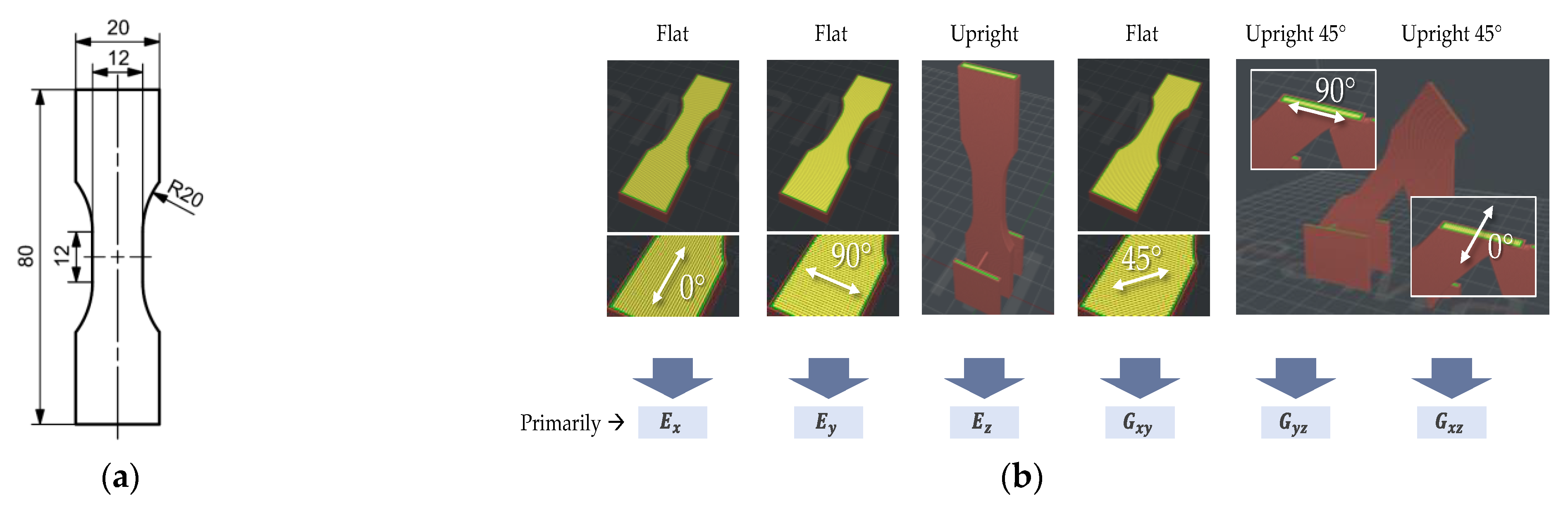
Figure 3a presents the specimen geometry used, which is a Becker tensile bar and can be used for both high-speed and quasi-static testing [34,35] and thus allows for flexibility for further extensions towards high-speed testing. In this contribution, only quasi-static testing is performed. Experiments at elevated strain rates and in the fatigue range have already been successfully carried out in [36,37] on injection-molded SFRP with this specimen geometry. The tensile bars have a thickness of 4 mm so these can be tested on testing equipment with a higher force range.
The orientation on the build platform and infill of the specimen are an extension of the work by Bellini et al. [25]. Six specimens are used overall, Figure 3b:
- The tensile bar is printed flat on the printing platform with longitudinal infill (Flat 0°, F0° in the following), intended to primarily yield Young’s modulus in longitudinal direction ;
- Same orientation, but with perpendicular infill (F90°) for Young’s modulus in perpendicular direction in-plane ;
- Upright position with infill printed in the same direction as F90°, thus called Upright 90° (U90°), intended to explain interlayer modulus ;
- Flat printed position with 45° infill within plane (F45°) for shear modulus ;
- Diagonally printed position (45° to plane) with parallel infill to walls, thus called U45°-90° for shear modulus ;
- And diagonally printed position, yet with perpendicular infill to walls (like F0°), thus called U45°-0° for shear modulus .
Thus, for all specimens, 0°-direction in infill is used when a Young’s modulus or shear modulus concerning the x-direction of the material model is to be calibrated; 90° in infill for y-direction; and 45° in in-plane infill or build orientation for shear. For each tpecimen, a FE simulation depicting both outer geometry and infill is set up using the approach presented by the authors [39]. This process is described in Section 2.2.
The specimens were printed on a Raise3D Pro2 Plus FLM printer using a 0.6 mm nozzle (instead of smaller nozzles, to avoid clogging by short fibres) at 254 °C nozzle and 60 °C build plate temperature. Infill extrusion width percentage was 105% (overlap/negative air gap). As printer filament, 1.75 mm FormFutura CarbonFil (15 wt.% short carbon fibre reinforced PETG [40]) filament was used. Support and wall/infill structure were both printed using CarbonFil and separated manually. Printing speed was 40 mm/s for most parts and reduced to 20 mm/s for upright samples. Both calibration (tensile) and validation (XX-rib) specimens were printed with this same slicing template.
2.2. Simulation and Fitting of Orthotropic Material Parameters
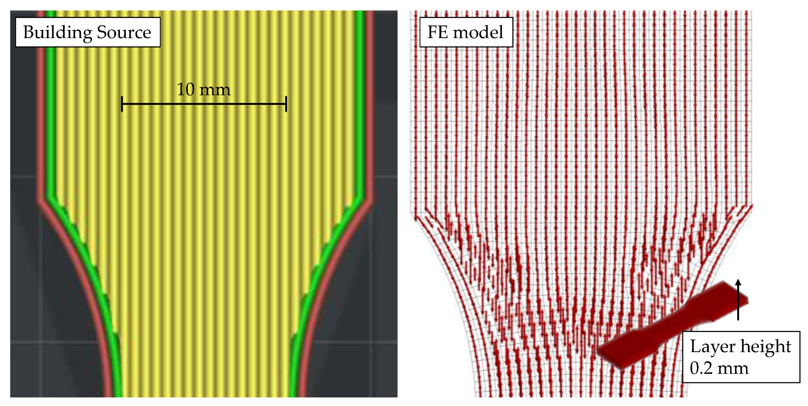
The setup of the specimen simulations is based on two inputs: First, the real, printed Becker samples are measured in each dimension (length, width, height) and the mean over each specimen geometry’s samples dimensions is calculated (one length, width, and height for each specimen geometry F0°, F90°, U90°, F45°, U45°-90° and U45°-0°, respectively). CAD models with this real geometry are created–not of the nominal geometry; thus, later FE models fit the real geometries appropriately. Second, for each geometry, the building source (G-Code) from the slicing software is used as an input for the mapping of inner material trajectories. A FE model is set up with in-plane element size aligned with printed beads width (for the 0.6 mm nozzle utilized this is approximately 0.6 mm). Element layer heights in z-direction, in turn, correspond to printed layer heights of 0.2 mm. Thus, infill orientation can be depicted properly. Boundary conditions and loads are configured as in the physical experiment (fixed at the bottom, given displacement at the top area on both sides of the tensile bar). The final, mapped FE model for F0° is presented in Figure 4 alongside the extrusion paths from building source (outer walls in red, inner walls in green, infill in yellow).
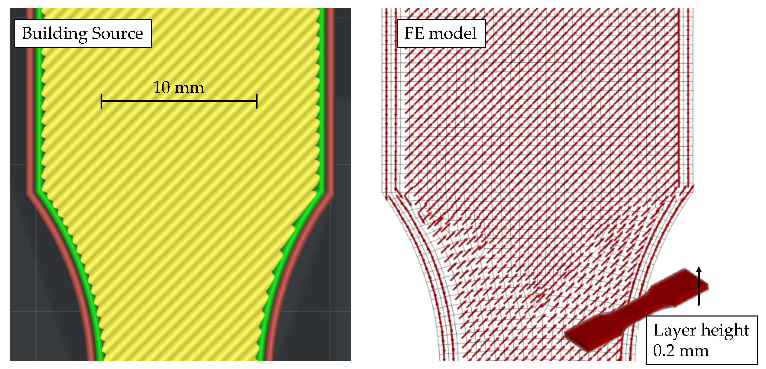
The mapping of the extrusion paths from building source to the FE mesh show accordance in the areas of both wall (red/green) and infill (yellow). The same procedure is repeated for all other specimen orientations and infill patterns, as presented again exemplarily for F45° in Figure 5.
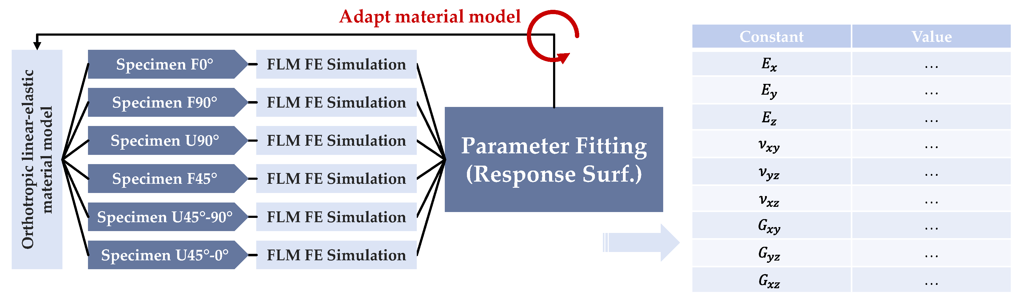
Based on the six simulations, a fitting workflow is established, Figure 6. All specimen simulations are fed by the same orthotropic material model with its nine constants, which at the same time constitute the design variables for fitting.
For each of the specimen simulations, ten equidistant force-displacement-pairs, longitudinal strain-displacement-pairs, and transverse strain-displacement pairs (overall pairs) are extracted as outputs and compared to the averaged corresponding pairs of the respective experiments. The method to select these ten force-displacement pairs follows the steps below:
- Average the experiment data to obtain one force-displacement, one longitudinal strain-displacement, and one transverse strain-displacement curve for each of the six samples (18 curves total).
- Find the linear parts of the curves (from displacement = 0 to the end of the linear part), for reference of the experimental data see the results section (Section 3). This is done to allow the linear elastic model to fit to the actual linear section of the curve. To obtain this linear limit, the following steps were taken and are proposed as a solution: (1) Smooth the average curve by a moving average of 10 measurement pairs; (2) Calculate the slope between each curve point and its predecessor ; (3) Calculate the curvature by calculating the “slope’s slope”, in turn; and (4) find the first occurrence where the percentage difference in curvature is smaller than a certain threshold (here, 0.75% were used arbitrarily). The threshold depends on the desired “strictness” of linearity; the smaller, the stricter. To avoid considering the initial, rather noisy data within the first part of the experiment, the linearity detection starts after 10% of the experiment curve data. (4) Finally, 10 equidistant displacement points are selected from the linear span of deformation . Using a mapping function, the closest (minimum-difference) data pairs from the averaged, but still discrete experiment data are selected.
Results of this method for stress-strain curves are depicted in Figure 7 for the six specimen and in detail for U90° (right). Detected linear curve segments are shown as red-dashed lines, the equidistant value pairs scattered as red “x” markers.
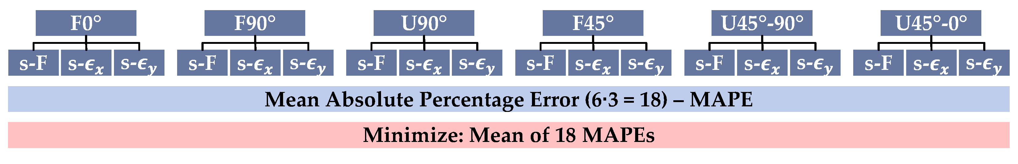
Concerning the fitting itself, for each specimen an error measure between simulation and experiment curves is calculated for later comparison of fitted material models. Mean Absolute Percentage Error (MAPE) is selected as error measure, as it allows condensation of individual errors into one aggregate number per geometry and pair category (that is, three error measures per specimen, for reaction force, longitudinal, and transverse strain, respectively; error measures in total) and does not “average out” negative and positive deviations between simulation and experiment, as simple Mean Percentage Error (MPE) would. At the same time, the percentage error is independent of scale, which is important as strains are much smaller in absolute terms than forces. Overall fitting target is then to minimize the unweighted average of all error measures. That omission of weighting implies that equal importance is paid to all specimen geometries and their quantitative results (force, longitudinal/transverse strains). Fitting of the strains alongside force-displacement further allows to calibrate the Poisson’s ratios of the orthotropic material model in addition to the Young’s and shear moduli. An overview of the aggregation approach is finally presented in Figure 8.
For fitting of the material parameters, response surface based optimization from ANSYS Software [41] is used with the built-in multi-objective genetic algorithm (MOGA) for optimization. Force value “tolerance” for target value search in the algorithm was set to 10 N (<1% of expected force values), strain tolerance to 0.01% (<1% of expected strain values).
2.3. Validation
To evaluate the prediction quality of the calibrated material model, a three-point bending test is compared in experiment and simulation for validation. The specimen geometry used is a cross-ribbed beam called XX-rib, dimensions specified in Figure 9a and CAD model in Figure 9b, manufactured upright. Because the FLM-printed specimens show quite large deviations from the nominal shape, these are measured at several points. For the simulation, wall thicknesses are used which correspond to the average geometric dimensions of all measured specimens. This average specimen geometry has a length of 60.3 mm, a height of 8.5 mm and a width of 20.6 mm. The wall thickness of the cover plate is 2.6 mm, that of the side walls 2.1 mm and that of the ribbing 2.2 mm. The setup of the simulation, with the specimen resting unrestrained on the supports and a load applied by the flexure fin, is shown in Figure 9c. The contact interfaces between the steel tool and the specimen are modeled with a coefficient of friction of .
2.4. Conduct and Evaluation of Experiments
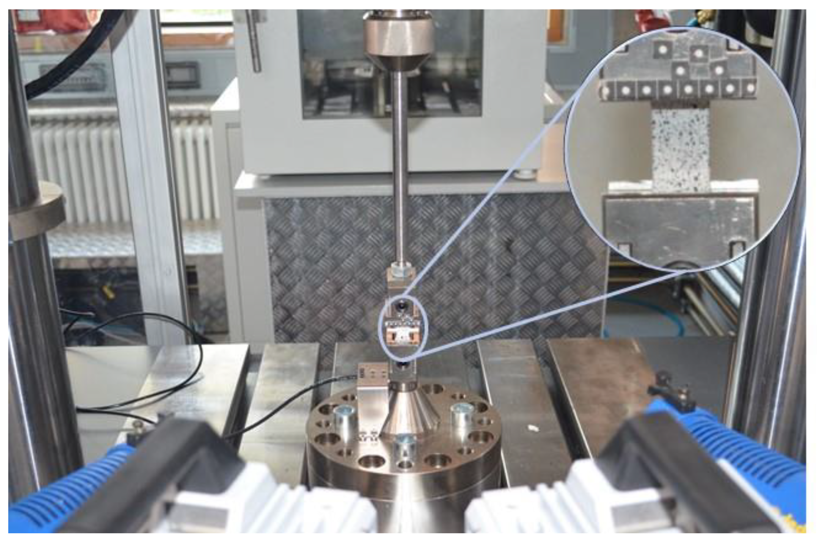
The experiments to characterize the tensile specimens are carried out on a servo-hydraulic high-speed testing machine, Zwick HTM 5020. It allows tests to be conducted with loads of up to 50 kN and test speeds from the quasi-static range to 20 m/s. For the characterization presented here, a load cell suitable for forces up to 10 kN is used, which provides a sufficiently fine resolution of the low test forces to be expected.
The test setup is shown in Figure 10 and consists essentially of the lower, fixed clamping and the upper clamping, which is set in motion by the hydraulic piston from the crosshead. The optical measuring system GOM ARAMIS 3D HHS is used for contactless measurement of the movement of the upper clamping and the deformation of the specimen itself. The measuring system works according to the principle of digital image correlation (DIC), whereby the strain on the sample surface is measured by distorting a stochastic grey value pattern, the displacement of the upper fixture as a translation of discrete points.
The tensile tests are performed at a speed of 1 mm/s and recorded at a sampling rate of 1 kHz. The experiments of the targeted 6 specimen geometries are repeated 5 times each. Force values are recorded image-synchronously so that a load value is available for each recorded deformation state. This allows the creation of force-displacement as well as stress-strain curves. From the knowledge of the stress-strain relationship, Young’s modulus and Poisson’s ratio are calculated for the different specimen types following DIN EN ISO 527 [42,43]. The stiffness values obtained in this way are to be used as starting values for the subsequent optimization of the material model.
Since several specimen types have a border of the parallel area pointing in the longitudinal dsirection even if the orientation is different (e.g., visible in Figure 5), a correction of the measured Young’s modulus must be carried out for these specimens. This treats the parallel perimeter area and the differently oriented inner area like a parallel connection of springs. The respective area fractions of the total sample cross section are obtained from an analysis of the fracture surfaces of the destroyed samples. The following applies here:
With being the overall stiffness of the specimen F90° including longitudinal borders and a transversal infill, and being the stiffness in each direction. and are the respective are fractions of the border layers and the filling.
In this way, the Young’s moduli in x, y and z directions are calculated from the experiments on samples F0°, F90° and U90°. To determine the values of the shear modulus, the samples F45°, U45°-90° as well as U45°-0° are used for the off-axis tensile test as well as the Poisson’s ratio [44]. In accordance to Bellini et al. [25], the shear modulus is calculated from the measured stiffness as follows:
Although a linear elastic material model will be calibrated and used in the simulation, it is expected that the material behavior in the real experiments be noticeably non-linear. Therefore, the linear range found according to Figure 7 is used for the calibration of the material model.
To validate the material model, 3-point bending tests are carried out on cross-ribbed beams, called XX-rib, cf. Figure 9. The steel supports with a spacing of 46 mm are filleted with a radius of 2 mm, the fin with a radius of 5 mm. The resulting force is measured by using a load cell in the upper piston. The indentation of the fin, like the movement of the upper restraint of the tensile tests, is measured by means of digital image correlation, resulting in force-displacement curves. The validation experiment is repeated for 7 specimens each.
3. Results
This section presents the results of the investigations carried out, namely those of the experiments necessary for the calibration and the parameter fitting in the simulation. Furthermore, the results of experiments and simulations for validation are presented.
3.1. Calibration
3.1.1. Experiments
The results of the tensile tests carried out are summarized in Figure 11 in the form of force-displacement curves (a) and stress-strain curves (b) for the different orientations.All curves displayed are averaged over the number of repeated experiments. The highest results by far are achieved by the sample F0°, reinforced in the tensile direction, with an average maximum stress of 85.8 MPa. As expected, the upright-printed sample U90° performs weakest, showing a mean maximum stress of 18.3 MPa. When looking at the curves, an overall non-linear behavior is noticeable, with a linear range being identified for all samples at the beginning of the loading. This linear range is used to calibrate the Young’s moduli of the material model.
According to the calculation procedures described in Section 2.4, the Young’s moduli and shear moduli as well as the Poisson’s ratios were determined as shown in Table 1. The values shown are averaged over the number of experiments.
The parameters determined in this way are used as starting values for the subsequent simulative parameter fitting.
3.1.2. Simulation and Parameter Fitting
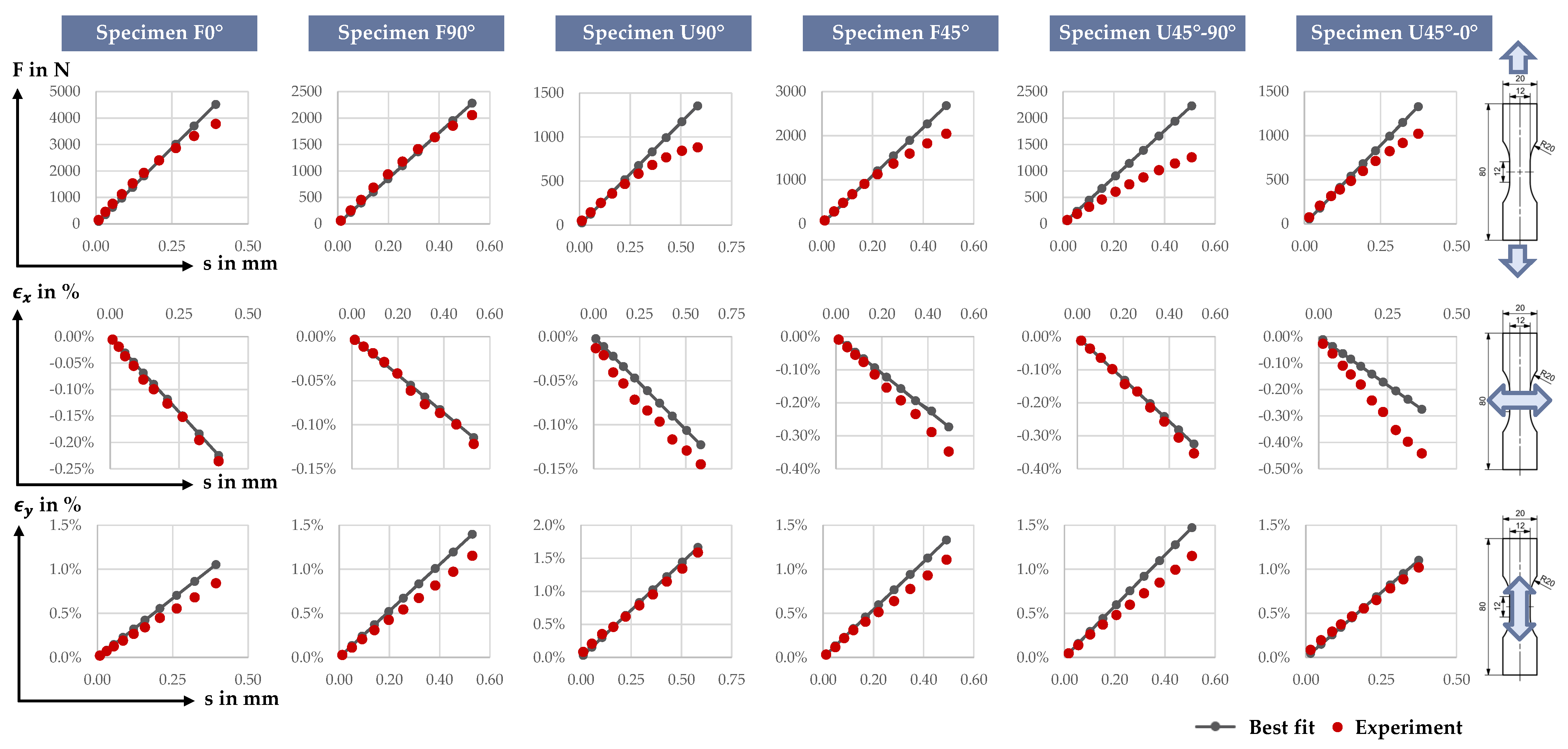
Following the description in Section 2.2, for each of the six specimens, displacement-force, displacement-longitudinal strain, and displacement-transverse strain curves (totalling curves) were fitted at 10 displacement points (i.e., output parameters overall) using the 9 orthotropic constants of the material model as input parameters for all the six FE specimen setups. The displacement-strain curves are intended to derive the Poisson’s ratios primarily, while the displacement-force curves should explain Young’s and shear moduli. Figure 12 presents the results for each of the 18 curves with the specimen geometries listed horizontally and the three curve types vertically.
Overall, the fitting quality is adequate (MAPE < 20%) in most cases, as also presented quantitatively in Table 2. The material parameters of the best response surface method optimized fit are given in Table 3. In comparison to the start values (in italics in Table 3), larger deviations occur in . This seems logical as in the experimental specimen, there is a certain fraction of 0° walls in the cross section which overstates longitudinal stiffness in comparison to which depicts purely 90° infill (no walls). The analytical estimation displayed in Equation (1) seems to still overestimate the value. Poisson’s ratio and shear modulus are greatly increased during the fitting, which can be explained again by a large proportion of walls within the cross section of specimen U45°-0° (refer Figure 3b, right). U45°-0° is thus not sufficient to explain the XZ-constants. In comparison, expectedly, the completely-0° specimen F0° yields a relative fitted-measured-difference in of just −0.7% (8153 MPa fitted vs. 8212 MPa measured). For the lying-down and upright specimens F0°, F90°, U90° and F45° fitting is visually accurate in the graphs above overall. For F90° the MAPE in force and transverse strain are higher in comparison (25% and 35%, respectively). In terms of displacement-force, this is explainable as the detected “linear” curve segment is not really linear and shows a disadvantage of the “linear-detection” method: small changes in local curvature might, nonetheless, yield large overall curvature. In terms of transverse strain, the poorer fitting might be due to a compromise of the optimization of other parameters (e. g., longitudinal stiffness of walls in F0°). For the upright-diagonal specimen U45°-90°, displacement-force yields poorer fitting quality, partly due to the linearity issue (first three data points are fitted quite well with MAPE < 25%). For U45°-0°, transverse strain results are less precisely fitted, in accordance with U90° (large influence of 0° infill).
To scrutinize whether specimen geometries influence the desired parameters (Figure 3b) and whether the measured strains at least partly determine Poisson’s ratios, a correlation coefficient analysis is conducted using sample points from the response surface. Correlation coefficients between the input parameters and orthotropic constants are given in Table 4.
3.2. Validation
3.2.1. Experiments
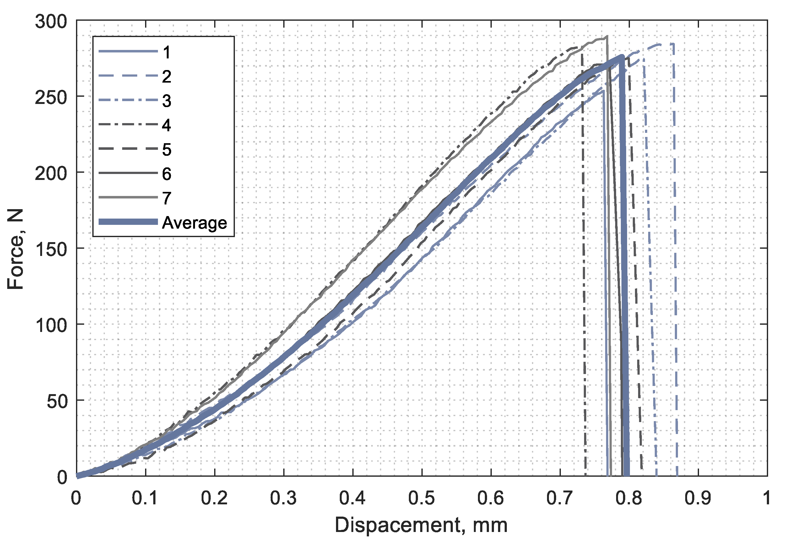
The results of the bending tests are shown as force-displacement curves in Figure 13. It shows the averaged curve as well as the results of the individual tests, which have a certain scatter. The values of the maximum force are between 253 N and 289 N, the indentation reached between 0.73 mm and 0.86 mm. For the averaged curve, the maximum force is 276 N at an indentation of 0.79 mm.
The scatter of the individual experiments may be due to the geometric inequality and the deviating wall thicknesses of the additively manufactured samples. The averaged force-displacement curve is therefore used for the subsequent comparison with the simulation.
3.2.2. Simulation and Material Model Validation
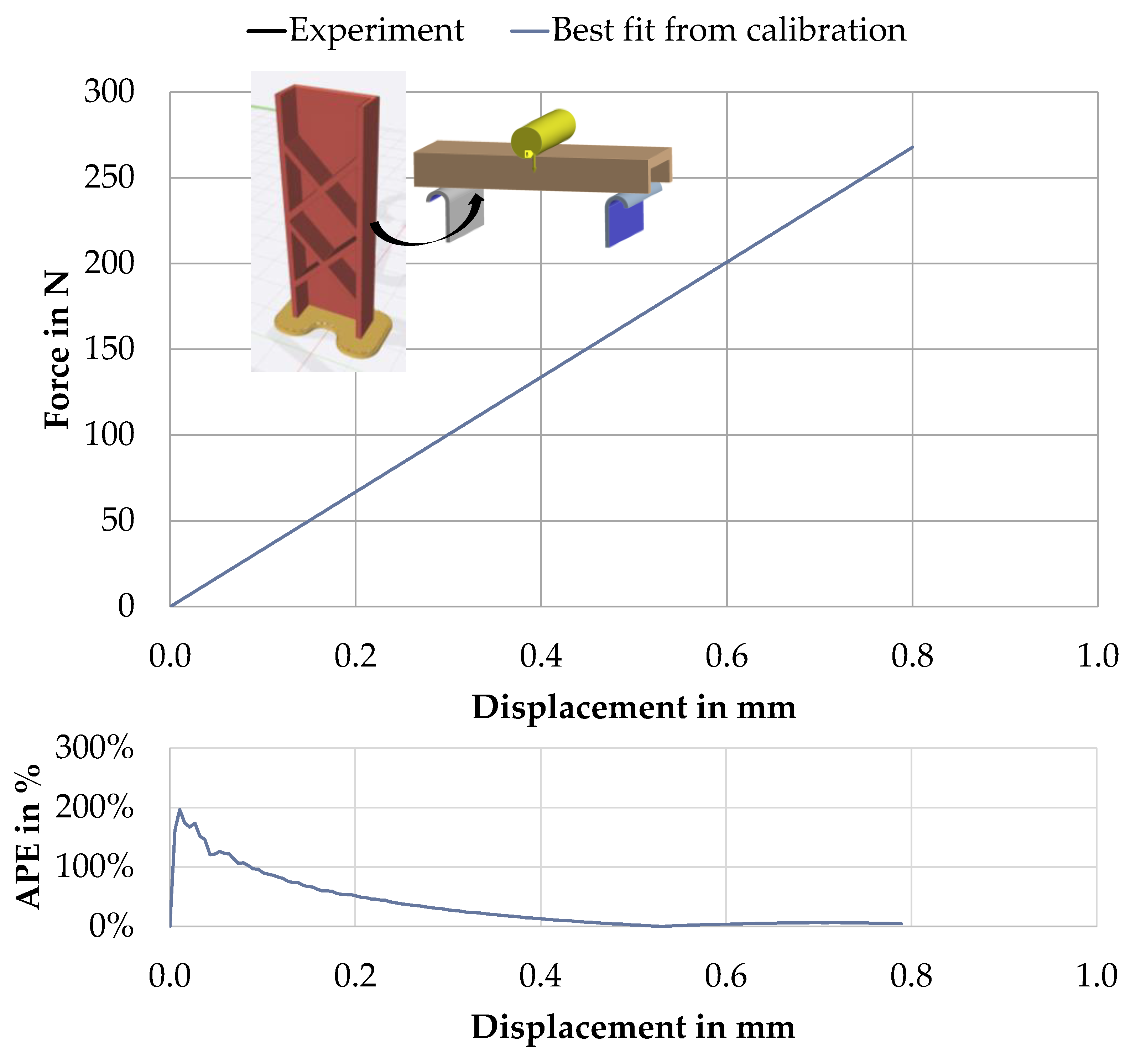
Application of the fitted material model (Table 3) in the simulation of the XX-rib demonstrator yields the following force-displacement-curve, Figure 14.
Despite the XX-rib being printed in an upright manner and tested under bending–thus, transferring the load rather inhomogeneously both between and within layers under different infill and contour directions–the overall match between simulation and experiment is considered satisfactory (overall MAPE is 35%). Within 0 mm to 0.5 mm displacement (maximum longitudinal strain approximately 1.8%) the FE model stiffness is higher than the physical demonstrator’s stiffness. In this interval, the majority of the overall MAPE is caused (≈52.6%). From there on to 0.8 mm displacement, this is inversed. The MAPE in this interval is small (≈4.0%).
4. Discussion: Advantages, Disadvantages, and Open Research Questions of Simultaneous Parameter Fitting
Simultaneous fitting of the orthotropic material constants offers advantages in comparison to the frequently pursued simple testing of longitudinal and transverse Young’s modulus, which merely yields these two constants (plus Poisson’s ratio in-plane, if measured): (1) A comprehensive, orthotropic, linear elastic material model with its 9 constants can be derived; (2) The obtained material model is capable of predicting the structural behavior under more complicated build direction, load case and wall/infill preconditions, as was demonstrated for the XX-rib demonstrator; (3) The approach is systematic, based on FLM-printable tensile test specimen. It is fully simulation-based and, therefore, integrable into digital workflows within product development.
The printing effort for the elaborate tensile specimens, especially U45°-0° and U45°-90° with their large proportion of support structures, constitutes a downside of the approach; moreover, for stability, both specimens require printed walls which in the case of U45°-0° are largely orthogonal to the desired infill direction.
Overall simulation effort is satisfactory and can be done on a regular workstation within a few hours, as the RSM allows for a limited number of simulations to obtain the response surface (instead of, for example, direct optimization using a simulation solver run at a time for each parameter set update). Naturally, the linear elastic material model only allows for linear simulation outcomes and, therefore, only a limited precision at approximating real, non-linear XX-rib specimen behavior; however, prediction quality appears satisfactory.
Open research questions are therefore: (i) Other, more easily printable specimen for deriving and should be conceived to simplify and accelerate printing (less support) as well as interpretation of fitting results (less orthogonal-wall proportion in U45°-0°, thus more direct derivation of ). This measure would improve fast applicability of the approach. (ii) The linearity measure could be improved to account for slow, but steady variations in curvature change. (iii) A more sophisticated material model than linear elastic could be fitted to better account for the actual, non-linear FLM material behavior. (iv) Other demonstrator parts should be tested in the future to have more reliable data on prediction quality. (v) Process parameter influence on the structural behavior and material model should be scrutinized more deeply, as these have a significant influence in this regard [10] and are frequently adapted, for example to minimize warping [45]. (vi) For future work, it should furthermore be checked whether an experimental model validation is also possible with further tensile tests, for example with other specimen geometries, in order to enable the validation in laboratories where there are no possibilities to carry out bending tests. (vii) Finally, it will be essential to carry out investigations in the area of fatigue in order to ensure the long-term, operationally safe use of components made of fibre reinforced FLM materials.
5. Conclusions
FLM material models play a significant role in designing and ensuring the functional properties of structural parts. In this contribution, a systematic approach to derive orthotropic FLM material models was motivated, described, and applied using 15 wt.% short carbon fibre reinforced PETG filament (FormFutura CarbonFil). For calibration, six specimen geometries intended to explain the six moduli of the orthotropic material model were conceived and printed as further development of Bellini et al. [25]. All orthotropic constants were fitted simultaneously using the RSM method. Quantitatively, correlation analysis showed the intended correlation between specimen geometry reaction forces and the respective material parameters. Poisson’s ratios were fitted using longitudinal and transversal, averaged experimental strain data. The correlation analysis indicated that multiple specimen reaction forces were influenced by these ratios. Overall calibration quality was satisfactory with the majority of MAPEs below 20%. Validation was conducted using an upright-printed, rib-stiffened bending specimen (“XX-rib”) to ensure that orthotropic constants apart from “simple” longitudinal and transversal Young’s moduli are necessarily used to explain material behavior. Validation quality was satisfactory observing the fitting graph. MAPE was higher for lower displacements and small for larger displacements, showing the original non-linear behavior of the real specimen. In the described way, material parameters of an orthotropic model were identified, which are summarized in Table 5. The model has been successfully validated for longitudinal strains of up to 1.8% and can be used for simulation.
The overall approach looks promising to be used as a systematic approach for deriving FLM material models in virtual product development. Open research questions were outlined.
Author Contributions
Conceptualization, C.W., H.V. and S.W.; Data curation, C.W. and H.V.; Formal analysis, C.W. and H.V.; Funding acquisition, S.W.; Investigation, C.W. and H.V.; Methodology, C.W. and H.V.; Project administration, S.W.; Resources, C.W. and H.V.; Software, H.V.; Supervision, S.W.; Validation, C.W. and H.V.; Visualization, C.W. and H.V.; Writing—original draft, C.W. and H.V.; Writing—review and editing, C.W., H.V. and S.W. All authors have read and agreed to the published version of the manuscript.
Funding
We acknowledge financial support by Deutsche Forschungsgemeinschaft and Friedrich-Alexander-Universität Erlangen-Nürnberg within the funding programme “Open Access Publication Funding”.
Acknowledgments
The authors would like to thank the students Robert Schade, Markus Lindner and Dominik Klose for their valuable contributions in the printing, testing and simulation of the material specimens used in this work.
Conflicts of Interest
The authors declare no conflict of interest.
References
- Lachmayer, R.; Lippert, R.B.; Fahlbusch, T. 3D-Druck Beleuchtet; Springer: Berlin/Heidelberg, Germany, 2016. [Google Scholar]
- Thompson, M.K.; Moroni, G.; Vaneker, T.; Fadel, G.; Campbell, R.I.; Gibson, I.; Bernard, A.; Schulz, J.; Graf, P.; Ahuja, B.; et al. Design for Additive Manufacturing: Trends, opportunities, considerations, and constraints. CIRP Ann. 2016, 65, 737–760. [Google Scholar] [CrossRef] [Green Version]
- Verein Deutscher Ingenieure. Additive Fertigungsverfahren: Grundlagen, Begriffe, Verfahrensbeschreibungen; 25.020(VDI 3405); Beuth Verlag: Berlin, Germany, 2014. [Google Scholar]
- Vajna, S.; Weber, C.; Zeman, K.; Hehenberger, P.; Gerhard, D.; Wartzack, S. CAx für Ingenieure: Eine Praxisbezogene Einführung, 3rd ed.; Springer Vieweg: Wiesbaden, Germany, 2018. [Google Scholar]
- Tan, P. Numerical simulation of the ballistic protection performance of a laminated armor system with pre-existing debonding/delamination. Compos. Part B Eng. 2014, 59, 50–59. [Google Scholar] [CrossRef]
- Rozylo, P. Failure analysis of thin-walled composite structures using independent advanced damage models. Compos. Struct. 2021, 262, 113598. [Google Scholar] [CrossRef]
- Brenken, B.; Barocio, E.; Favaloro, A.; Kunc, V.; Pipes, R.B. Fused filament fabrication of fiber-reinforced polymers: A review. Addit. Manuf. 2018, 21, 1–16. [Google Scholar] [CrossRef]
- Shofner, M.L.; Lozano, K.; Rodríguez-Macías, F.J.; Barrera, E.V. Nanofiber-reinforced polymers prepared by fused deposition modeling. J. Appl. Polym. Sci. 2003, 89, 3081–3090. [Google Scholar] [CrossRef]
- DeNardo, N.M. Additive Manufacturing of Carbon Fiber-Reinforced Thermoplastic Composites. Master’s Thesis, West Purdue University, Lafayette, IN, USA, 2016. [Google Scholar]
- Ning, F.; Cong, W.; Hu, Y.; Wang, H. Additive manufacturing of carbon fiber-reinforced plastic composites using fused deposition modeling: Effects of process parameters on tensile properties. J. Compos. Mater. 2017, 51, 451–462. [Google Scholar] [CrossRef]
- Kabir, S.M.F.; Mathur, K.; Seyam, A.-F.M. A critical review on 3D printed continuous fiber-reinforced composites: History, mechanism, materials and properties. Compos. Struct. 2020, 232, 111476. [Google Scholar] [CrossRef]
- Kolanu, N.R.; Raju, G.; Ramji, M. A unified numerical approach for the simulation of intra and inter laminar damage evolution in stiffened CFRP panels under compression. Compo. Part B Eng. 2020, 190, 107931. [Google Scholar] [CrossRef]
- Thomas, D.S.; Gilbert, S.W. Costs and Cost Effectiveness of Additive Manufacturing, NIST Special Publication 1176; NIST National Institute of Standards and Techology: Gaithersburg, MD, USA, 2014. [Google Scholar]
- Such, M.; Ward, C.; Potter, K. Aligned Discontinuous Fibre Composites: A Short History. JMC 2014, 2, 155–168. [Google Scholar] [CrossRef]
- Armiger, T.E.; Edison, D.H.; Lauterbach, H.G.; Layton, J.R.; Okine, R.K. Composites of Stretch Broken Aligned Fibers of Carbon and Glass Reinforced Resin. European Patent EP0272088A1, 15 December 1987. [Google Scholar]
- Parandoush, P.; Lin, D. A review on additive manufacturing of polymer-fiber composites. Compos. Struct. 2017, 182, 36–53. [Google Scholar] [CrossRef]
- Montero, M.; Roundy, S.; Odell, D.; Ahn, S.; Wright, P. Material Characterization of Fused Deposition Modeling (FDM) ABS by Designed Experiments. In Proceedings of the Rapid Prototyping and Manufacturing Conference, Cincinnati, OH, USA, 15–17 May 2001; pp. 1–21. [Google Scholar]
- Ahn, S.; Montero, M.; Odell, D.; Roundy, S.; Wright, P.K. Anisotropic material properties of fused deposition modeling ABS. Rapid Prototyp. J. 2002, 8, 248–257. [Google Scholar] [CrossRef] [Green Version]
- Wu, W.; Geng, P.; Li, G.; Di, Z.; Zhang, H.; Zhao, J. Influence of Layer Thickness and Raster Angle on the Mechanical Properties of 3D-Printed PEEK and a Comparative Mechanical Study between PEEK and ABS. Materials 2015, 8, 5834–5846. [Google Scholar] [CrossRef]
- Sood, A.K.; Ohdar, R.K.; Mahapatra, S.S. Experimental investigation and empirical modelling of FDM process for compressive strength improvement. J. Adv. Res. 2012, 3, 81–90. [Google Scholar] [CrossRef] [Green Version]
- Hernandez, R.; Slaughter, D.; Whaley, D.; Tate, J.; Asiabanpour, B. Analyzing the Tensile, Compressive, and Flexural Properties of 3D Printed ABS P430 Plastic Based on Printing Orientation Using Fused Deposition Modeling. In Solid Freeform Fabrication 2016, Proceedings of the 27th Annual International Solid Freeform Fabrication Symposium, Austin, TX, USA, 8–10 August 2016; Bourell, D.L., Crawford, R., Seepersad, C., Beaman, J.J., Fish, S., Harris, M., Eds.; University of Texas at Austin: Austin, TX, USA; pp. 939–950.
- Pei, E.; Lanzotti, A.; Grasso, M.; Staiano, G.; Martorelli, M. The impact of process parameters on mechanical properties of parts fabricated in PLA with an open-source 3-D printer. Rapid Prototyp. J. 2015, 21, 604–617. [Google Scholar] [CrossRef] [Green Version]
- Li, L.; Sun, Q.; Bellehumeur, C.; Gu, P. Composite Modeling and Analysis for Fabrication of FDM Prototypes with Locally Controlled Properties. J. Manuf. Process. 2002, 4, 129–141. [Google Scholar] [CrossRef]
- Matas, J.F.R. Modeling the Mechanical Behavior of Fused Deposition Acrylonitrile-Butadiene-Styrene Polymer Components. Master’s Thesis, University of Notre Dame, Notre Dame, IN, USA, 1999. [Google Scholar]
- Bellini, A.; Güçeri, S. Mechanical characterization of parts fabricated using fused deposition modeling. Rapid Prototyp. J. 2003, 9, 252–264. [Google Scholar] [CrossRef]
- Domingo-Espin, M.; Puigoriol-Forcada, J.M.; Granada, A.A.G.; Llumà, J.; Borros, S.; Reyes, G. Mechanical property characterization and simulation of fused deposition modeling Polycarbonate parts. Mater. Des. 2015, 83, 670–677. [Google Scholar] [CrossRef]
- Rodríguez, J.F.; Thomas, J.P.; Renaud, J.E. Mechanical behavior of acrylonitrile butadiene styrene fused deposition materials modeling. Rapid Prototyp. J. 2003, 9, 219–230. [Google Scholar] [CrossRef]
- Lee, C.S.; Kim, S.G.; Kim, H.J.; Ahn, S.H. Measurement of anisotropic compressive strength of rapid prototyping parts. J. Mater. Process. Technol. 2007, 187–188, 627–630. [Google Scholar] [CrossRef]
- Cantrell, J.T.; Rohde, S.; Damiani, D.; Gurnani, R.; DiSandro, L.; Anton, J.; Young, A.; Jerez, A.; Steinbach, D.; Kroese, C.; et al. Experimental characterization of the mechanical properties of 3D-printed ABS and polycarbonate parts. Rapid Prototyp. J. 2017, 23, 811–824. [Google Scholar] [CrossRef]
- Somireddy, M.; Czekanski, A. Mechanical Characterization of Additively Manufactured Parts by FE Modeling of Mesostructure. J. Manuf. Mater. Process. 2017, 1, 18. [Google Scholar] [CrossRef] [Green Version]
- Tekinalp, H.L.; Kunc, V.; Velez-Garcia, G.M.; Duty, C.E.; Love, L.J.; Naskar, A.K.; Blue, C.A.; Ozcan, S. Highly oriented carbon fiber–polymer composites via additive manufacturing. Compos. Sci. Technol. 2014, 105, 144–150. [Google Scholar] [CrossRef] [Green Version]
- Duty, C.E.; Kunc, V.; Compton, B.; Post, B.; Erdman, D.; Smith, R.; Lind, R.; Lloyd, P.; Love, L. Structure and mechanical behavior of Big Area Additive Manufacturing (BAAM) materials. Rapid Prototyp. J. 2017, 23, 181–189. [Google Scholar] [CrossRef]
- Love, L.J.; Kunc, V.; Rios, O.; Duty, C.E.; Elliott, A.M.; Post, B.K.; Smith, R.J.; Blue, C.A. The importance of carbon fiber to polymer additive manufacturing. J. Mater. Res. 2014, 29, 1893–1898. [Google Scholar] [CrossRef] [Green Version]
- Becker, F. Entwicklung Einer Beschreibungsmethodik für das Mechanische Verhalten Unverstärkter Thermoplaste bei Hohen Deformationsgeschwindigkeiten. Ph.D. Thesis, Martin-Luther-Universität Halle-Wittenberg, Halle, Germany, 2009. [Google Scholar]
- Kunkel, F. Zum Deformationsverhalten von Spritzgegossenen Bauteilen aus Talkumgefüllten Thermoplasten unter Dynamischer Beanspruchung. Master’s Thesis, Otto-von-Guericke-Universität Magdeburg, Magdeburg, Germany, 2017. [Google Scholar]
- Witzgall, C.; Wartzack, S. An Investigation of Mechanically Aged Short-Fiber Reinforced Thermoplastics under Highly Dynamic Loads. In Proceedings of the DFX 2016 27th Symposium Design for X, Jesteburg, Germany, 5–6 October 2016; pp. 135–146. [Google Scholar]
- Witzgall, C.; Giolda, J.; Wartzack, S. A novel approach to incorporating previous fatigue damage into a failure model for short-fibre reinforced plastics. Int. J. Impact Eng. 2022, 18, 104155. [Google Scholar] [CrossRef]
- IdeaMaker: 3D Slicer Software; Raise 3D Technologies I; Raise 3D Technologies, Inc.: Irvine, CA, USA, 2020.
- Völkl, H.; Mayer, J.; Wartzack, S. Strukturmechanische Simulation additiv im FFF-Verfahren gefertigter Bauteile. In KfAF 2019 Konstruktion für die Additive Fertigung 2019, 1st ed.; Lachmayer, R., Rettschlag, K., Kaierle, S., Eds.; Springer: Berlin/Heidelberg, Germany, 2020; pp. 143–157. [Google Scholar]
- FormFutura. CarbonFil. Available online: https://www.formfutura.com/shop/product/carbonfil-2788?category=458 (accessed on 26 January 2022).
- ANSYS; ANSYS Help; SAS IP, Inc.: Cheyenne, WY, USA, 2017.
- ISO 527-1:2012-06; Kunststoffe—Bestimmung der Zugeigenschaften—Teil 1: Allgemeine Grundsätze. ISO; Beuth: Berlin, Germany, 2012.
- DIN EN ISO 527-4 1997; Kunststoffe—Bestimmung der Zugeigenschaften—Teil 4: Prüfbedingungen für isotrop und anisotrop faserverstärkte Kunststoffverbundwerkstoffe. ISO; Beuth Verlag: Berlin, Germany, 1997.
- Pierron, F.; Vautrin, A. Accurate comparative determination of the in-plane shear modulus of T300/914 by the iosipescu and 45° off-axis tests. Compos. Sci. Technol. 1994, 52, 61–72. [Google Scholar] [CrossRef]
- Alsoufi, M.; El-Sayed, A. Warping Deformation of Desktop 3D Printed Parts Manufactured by Open Source Fused Deposition Modeling (FDM) System. Int. J. Mech. Mechatron. Eng. 2017, 17, 7–16. [Google Scholar]
Figure 1.
FLM printing: (a) Photo of short 15 wt.% carbon-fibre reinforced PETG-CF15 getting printed on a Raise3D Pro2 Plus (left) and corresponding schematic of FLM hot-end (right); (b) Illustration of various current FLM material modeling approaches as described in the text.
Figure 1.
FLM printing: (a) Photo of short 15 wt.% carbon-fibre reinforced PETG-CF15 getting printed on a Raise3D Pro2 Plus (left) and corresponding schematic of FLM hot-end (right); (b) Illustration of various current FLM material modeling approaches as described in the text.
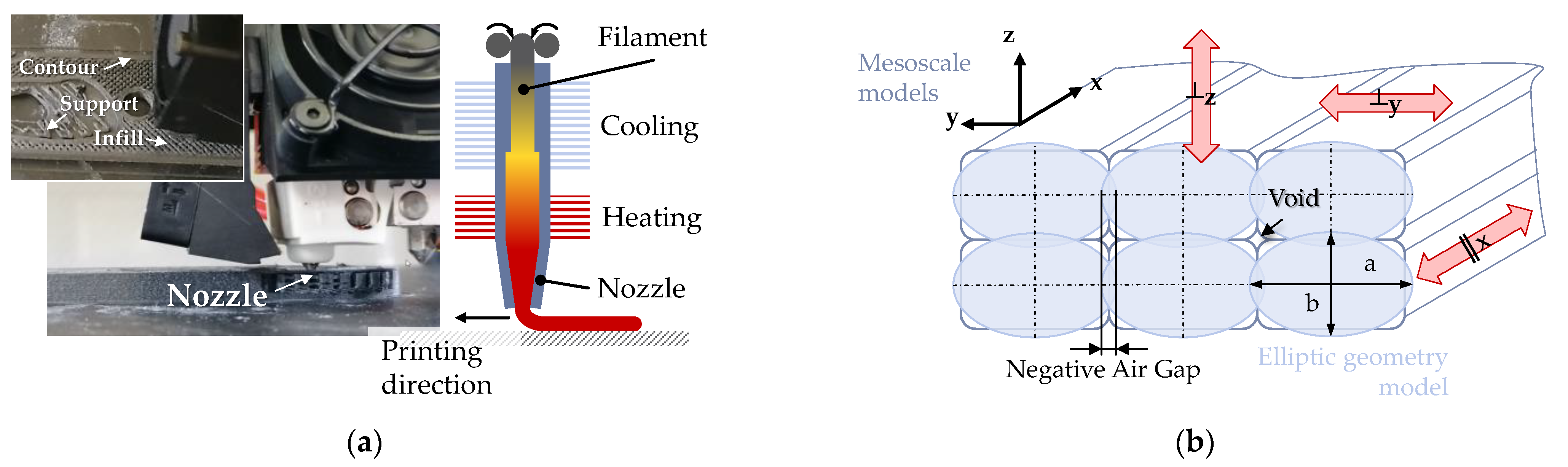
Figure 2.
Overarching methodology of this contribution.
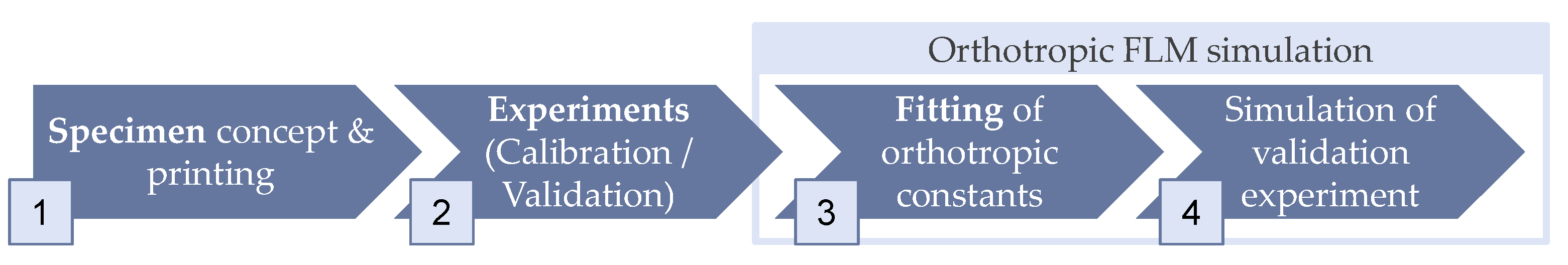
Figure 3.
Specimen geometries: (a) Becker specimen, technical drawing; (b) Specimen alignment and infill and their allocation to orthotropic constants, sliced by Raise3D ideaMaker software [38].
Figure 3.
Specimen geometries: (a) Becker specimen, technical drawing; (b) Specimen alignment and infill and their allocation to orthotropic constants, sliced by Raise3D ideaMaker software [38].

Figure 4.
Building source (G-Code, left) mapped to FE model (right) for the first specimen (F0°) using the approach presented by the authors [39].
Figure 4.
Building source (G-Code, left) mapped to FE model (right) for the first specimen (F0°) using the approach presented by the authors [39].

Figure 5.
Building source (G-Code, left) mapped to FE model (right) for the fourth specimen (F45°) using the approach presented by the authors [39].
Figure 5.
Building source (G-Code, left) mapped to FE model (right) for the fourth specimen (F45°) using the approach presented by the authors [39].

Figure 6.
Fitting method in detail: F = flat, U = upright specimen as in Figure 3.
Figure 6.
Fitting method in detail: F = flat, U = upright specimen as in Figure 3.

Figure 7.
Results of the detection of linear area within experimental averaged results.
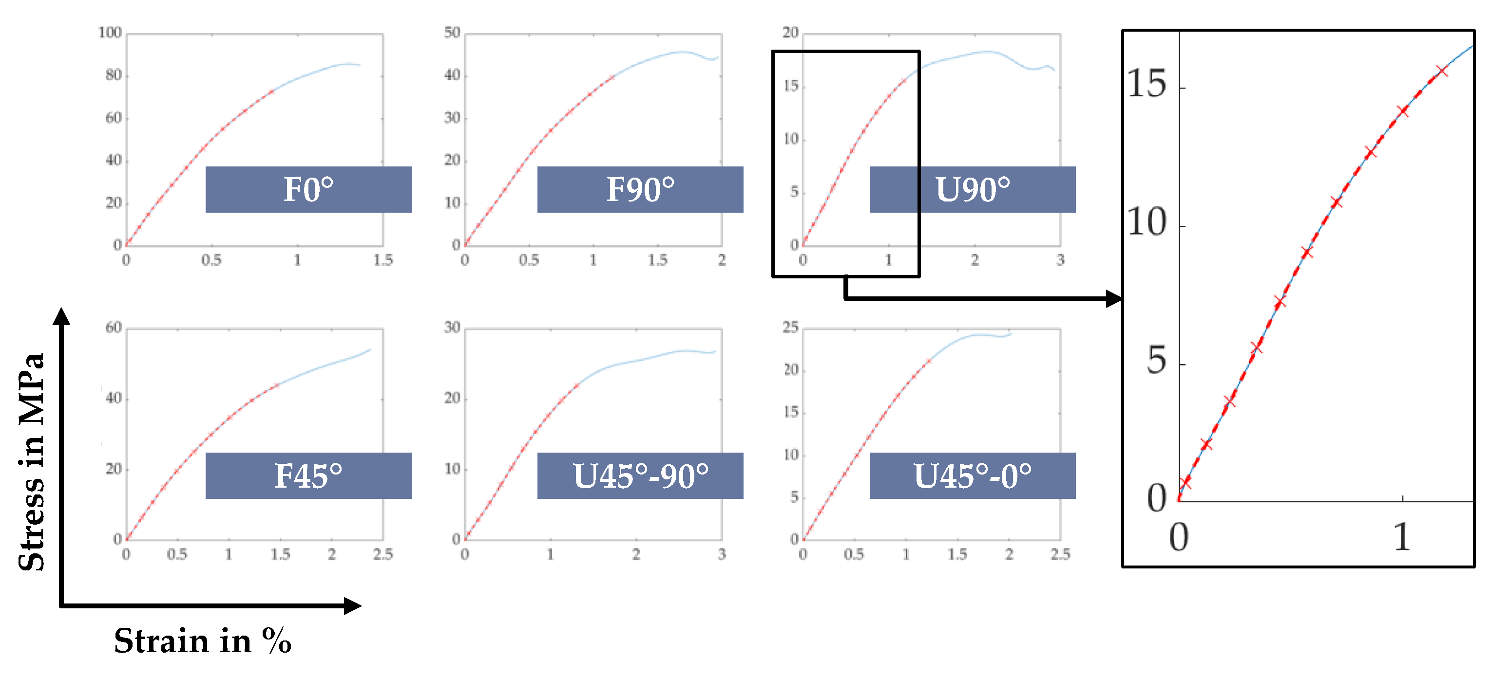
Figure 8.
Fitting: Aggregation of error measures in detail.

Figure 9.
XX-rib specimen geometry: (a) Specimen, technical drawing with main dimensions; (b) 3D model of and FLM-printed XX-rib specimen; (c) Bending load case for XX-rib specimen as applied in FE simulation. All contacts modeled using a coefficient of friction of .
Figure 9.
XX-rib specimen geometry: (a) Specimen, technical drawing with main dimensions; (b) 3D model of and FLM-printed XX-rib specimen; (c) Bending load case for XX-rib specimen as applied in FE simulation. All contacts modeled using a coefficient of friction of .
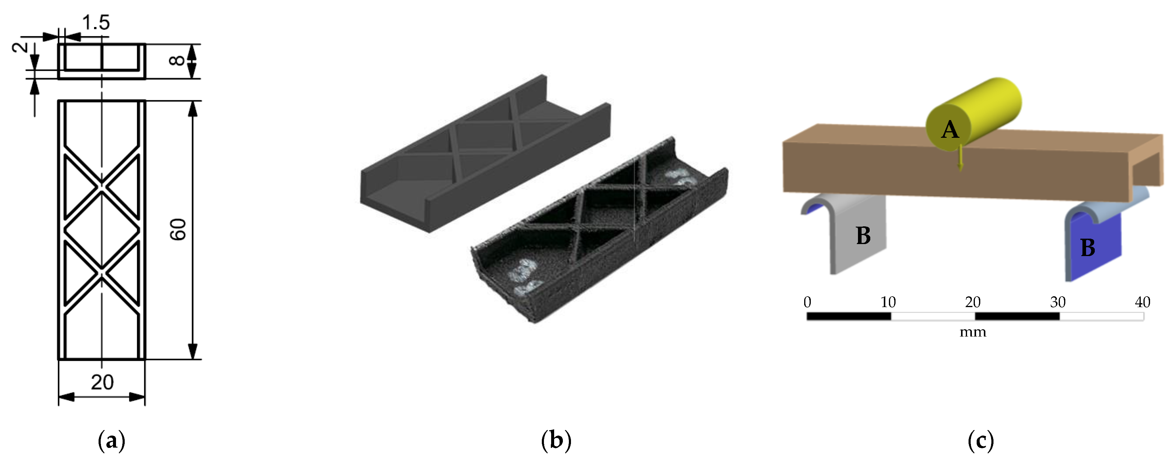
Figure 10.
Experimental setup with lower and upper clamping and speckled specimen.

Figure 11.
Results of experimental testing, averaged: (a) Force-displacement curves; (b) stress-strain curves.
Figure 11.
Results of experimental testing, averaged: (a) Force-displacement curves; (b) stress-strain curves.

Figure 12.
Fitting of force-displacement, transverse strain-displacement, and longitudinal strain simulation results (grey lines) to experimental results (ten red points each, identified above).
Figure 12.
Fitting of force-displacement, transverse strain-displacement, and longitudinal strain simulation results (grey lines) to experimental results (ten red points each, identified above).

Figure 13.
Force-displacement curves for single specimen 1 to 7 as well as averaged.

Figure 14.
Calibrated material model applied to upright-printed XX-rib specimen bending simulation compared to experimental result (force-displacement-curve above, average percentage error (APE) below; MAPE = 35%).
Figure 14.
Calibrated material model applied to upright-printed XX-rib specimen bending simulation compared to experimental result (force-displacement-curve above, average percentage error (APE) below; MAPE = 35%).


Table 1.
Material parameters determined from experiments, rounded.
| MPa | MPa | MPa | - | - | - | MPa | MPa | MPa |
|---|---|---|---|---|---|---|---|---|
| 8212 | 2615 | 1437 | 0.28 | 0.11 | 0.10 | 883 | 637 | 634 |
Table 2.
Mean absolute percentage error (MAPE) for each fitting, rounded to full percent (larger values than 30% are highlighted in grey).
Table 2.
Mean absolute percentage error (MAPE) for each fitting, rounded to full percent (larger values than 30% are highlighted in grey).
| F0° | F90° | U90° | F45° | U45°-90° | U45°-0° | |
|---|---|---|---|---|---|---|
| ) | 14% | 9% | 25% | 13% | 49% | 17% |
| 10% | 8% | 35% | 19% | 6% | 42% | |
| 20% | 21% | 14% | 14% | 21% | 12% |
Table 3.
Material parameters determined from simulation-based fitting, rounded. Experimental start values from Table 1 are repeated in italics.
Table 3.
Material parameters determined from simulation-based fitting, rounded. Experimental start values from Table 1 are repeated in italics.
| MPa | MPa | MPa | - | - | - | MPa | MPa | MPa |
|---|---|---|---|---|---|---|---|---|
| 8153 | 1949 | 1549 | 0.31 | 0.17 | 0.36 | 1096 | 642 | 1120 |
| 8212 | 2615 | 1437 | 0.28 | 0.11 | 0.10 | 883 | 637 | 634 |
Table 4.
Linear correlation coefficients between input and output parameters. Blue: Correlation coefficient or ; Orange: Correlation coefficient in [0.6; 0.8] or in [−0.8; −0.6].
Table 4.
Linear correlation coefficients between input and output parameters. Blue: Correlation coefficient or ; Orange: Correlation coefficient in [0.6; 0.8] or in [−0.8; −0.6].
| F (reaction forces at boundary) | F0° | 0.99 | 0.40 | 0.32 | 0.23 | 0.23 | 0.38 | 0.43 | −0.08 | 0.15 |
| F90° | 0.52 | 0.98 | 0.40 | 0.66 | 0.50 | 0.39 | 0.44 | 0.27 | 0.31 | |
| U90° | 0.24 | 0.35 | 1.00 | 0.53 | 0.61 | 0.65 | 0.63 | 0.32 | 0.44 | |
| F45° | 0.64 | 0.73 | 0.58 | 0.61 | 0.57 | 0.61 | 0.84 | 0.26 | 0.36 | |
| U45°-90° | 0.10 | 0.46 | 0.77 | 0.58 | 0.66 | 0.67 | 0.62 | 0.81 | 0.69 | |
| U45°-0° | 0.14 | 0.44 | 0.76 | 0.59 | 0.71 | 0.65 | 0.59 | 0.73 | 0.81 | |
(transverse mean strain) | F0° | 0.05 | −0.63 | −0.45 | −0.92 | −0.63 | −0.46 | −0.41 | −0.38 | −0.35 |
| F90° | 0.06 | −0.81 | −0.36 | −0.87 | −0.61 | −0.29 | −0.33 | −0.38 | −0.36 | |
| U90° | 0.05 | −0.09 | −0.82 | −0.47 | −0.64 | −0.80 | −0.56 | −0.42 | −0.50 | |
| F45° | −0.09 | −0.75 | 0.02 | −0.45 | −0.20 | 0.11 | 0.28 | −0.10 | −0.06 | |
| U45°-90° | −0.43 | −0.01 | −0.59 | −0.10 | −0.12 | −0.27 | −0.23 | 0.56 | 0.19 | |
| U45°-0° | −0.39 | −0.08 | −0.60 | −0.15 | −0.15 | −0.27 | −0.23 | 0.52 | 0.30 | |
(longitudinal mean strain) | F0° | −0.56 | 0.25 | 0.30 | 0.50 | 0.49 | 0.35 | 0.36 | 0.79 | 0.51 |
| F90° | −0.39 | 0.23 | 0.19 | 0.45 | 0.43 | 0.27 | 0.23 | 0.44 | 0.36 | |
| U90° | −0.29 | −0.05 | −0.48 | 0.07 | 0.20 | 0.01 | −0.10 | 0.45 | 0.41 | |
| F45° | −0.32 | 0.61 | 0.27 | 0.59 | 0.48 | 0.25 | 0.02 | 0.64 | 0.52 | |
| U45°-90° | 0.55 | −0.08 | 0.05 | −0.11 | −0.12 | 0.01 | 0.08 | −0.85 | −0.40 | |
| U45°-0° | 0.59 | 0.19 | 0.25 | 0.09 | 0.00 | 0.20 | 0.27 | −0.62 | −0.51 |
Young’s moduli , and correlate with F0°, F90° and U90° reaction forces nearly perfectly. Similarly, , and are closely linearly correlated with the reaction forces of F45°, U45°-90° and U45°-0°. Poisson’s ratios correlate with the transverse strains especially of F0°, F90° and U90° (transverse strain is measured with negative sign, thus smaller – larger absolute – transverse strain correctly correlates with larger ratios). The former also correlate considerably with reaction forces. In contrast to Young’s moduli, no clear assignment of a single, individual specimen to a certain ratio can be made. Shear modulus positively correlates with longitudinal strain for F0° and F45° and negatively with longitudinal strain for U45°-90°. Young’s modulus also correlates with the longitudinal strain of F45°. Longitudinal strain correlation is very much dependent on the overall geometry and infill (displacement is pre-defined in the FE model) and overall variations are small (10% variation in yields about 1% variation in of F90°, for example).
Table 5.
Overview of the identified material parameters for 15 wt.% short carbon-fibre reinforced PETG filament (Formfuture CarbonFil).
Table 5.
Overview of the identified material parameters for 15 wt.% short carbon-fibre reinforced PETG filament (Formfuture CarbonFil).
| MPa | MPa | MPa | - | - | - | MPa | MPa | MPa |
|---|---|---|---|---|---|---|---|---|
| 8153 | 1949 | 1549 | 0.31 | 0.17 | 0.36 | 1096 | 642 | 1120 |
Publisher’s Note: MDPI stays neutral with regard to jurisdictional claims in published maps and institutional affiliations. |
© 2022 by the authors. Licensee MDPI, Basel, Switzerland. This article is an open access article distributed under the terms and conditions of the Creative Commons Attribution (CC BY) license (https://creativecommons.org/licenses/by/4.0/).
Share and Cite
MDPI and ACS Style
Witzgall, C.; Völkl, H.; Wartzack, S. Derivation and Validation of Linear Elastic Orthotropic Material Properties for Short Fibre Reinforced FLM Parts. J. Compos. Sci. 2022, 6, 101. https://doi.org/10.3390/jcs6040101
AMA Style
Witzgall C, Völkl H, Wartzack S. Derivation and Validation of Linear Elastic Orthotropic Material Properties for Short Fibre Reinforced FLM Parts. Journal of Composites Science. 2022; 6(4):101. https://doi.org/10.3390/jcs6040101
Chicago/Turabian StyleWitzgall, Christian, Harald Völkl, and Sandro Wartzack. 2022. "Derivation and Validation of Linear Elastic Orthotropic Material Properties for Short Fibre Reinforced FLM Parts" Journal of Composites Science 6, no. 4: 101. https://doi.org/10.3390/jcs6040101