Article

Systematic Approach for Finite Element Analysis of Thermoplastic Impregnated 3D Filament Winding Structures—Advancements and Validation

1
Fraunhofer Institute for Chemical Technology, Department of Polymer Engineering, Joseph-von-Fraunhofer-Str. 7, 76327 Pfinztal, Germany
2
Karlsruhe Institute of Technology, Institute of Vehicle System Technology, Rintheimer Querallee 2, 76131 Karlsruhe, Germany
*
Author to whom correspondence should be addressed.
J. Compos. Sci. 2022, 6(3), 98; https://doi.org/10.3390/jcs6030098
Submission received: 26 February 2022 / Revised: 13 March 2022 / Accepted: 15 March 2022 / Published: 19 March 2022
(This article belongs to the Special Issue Characterization and Modelling of Composites, Volume II)

Abstract

:
This work aims to enhance and validate a systematic approach for the structural finite element (FE) analysis of thermoplastic impregnated 3D filament winding structures (fiber skeletons). The idealized modeling of geometrically complex fiber skeletons used in previous publications is refined by considering additional characteristic dimensions and investigating their mechanical influence. Moreover, the modeling approach is transferred from the meso- to the macro-level in order to reduce modeling and computational effort. The properties of meso- and macro-level FE models are compared using the example of simple loop specimens. Based on the results, respective application fields are defined. In the next step, the same modeling approach is applied to a more complex, three-dimensional specimen—the inclined loop. For its macro-level FE model, additional material characterization and modeling, as well as enhancements in the modeling of the geometry, are proposed. Together with previously determined effective composite properties of fiber skeletons, these results are validated in experimental tensile tests on inclined loop specimens.

1. Introduction

The 3D filament winding technology, also referred to as 3D Skeleton Winding technology (3DSW), is a design and production approach that allows lightweight potentials to be exploited to a particularly high degree. Its concept consists of winding thermoset or thermoplastic impregnated reinforcement fibers (e.g., glass or carbon fibers) onto a winding form, whereby (after curing or solidification of the polymer matrix) a so-called fiber skeleton is created. In comparison to the conventional filament winding process for the production of rotationally symmetric composite structures, the robot-based coreless 3D filament winding process offers greater geometric flexibility, allowing more complex, topology-optimized fiber skeletons to be realized. The impregnated fibers are usually wound around load introduction locations and support points (mostly implemented as metallic inserts) so that the fiber orientation is ideally aligned with the load paths. This allows occurring loads to be transferred directly into the continuous fibers in a form-fit manner, leading to high utilization of the fibers’ mechanical properties. Depending on the application, the fiber skeletons are used either as pure skeletal structures [1,2,3] or as local reinforcements within molded parts or laminates [4,5,6]. In both cases they generally serve to carry significant mechanical loads while minimizing the component’s mass [4,7,8].
Quantitative methods are needed that allow precise estimates of the fiber skeletons’ load bearing capacity and load-dependent deformation. While the mechanical behavior of wound ring reinforcements under internal pressure (with a constant, rectangular cross-sectional area) can be estimated on the basis of analytical equations [9], finite element (FE) analysis is generally used for the structural assessment of more complex winding structures. Depending on the size of the fiber skeleton considered and the failure modes investigated, different FE modeling approaches are suitable. In the simulation of large fiber skeletons (e.g., lightweight installation profiles, ship cabins or building structures) highly simplified geometry models are used. An overview of this modeling approach is given in [10]. As can be seen in [1,2,11,12,13] the fiber strings are usually modeled as one-dimensional rod or beam elements, while the fiber deflection points are represented by rigid connections of these elements. This approach enables precise estimates of elastic deformations of large wound trusses at low modeling and computational effort. However, it is not suited for precise simulations of the failure mechanisms typically occurring at the fiber deflection points that usually determine the fiber skeletons’ bearing capacity under tensile loading [8,9,14]. Since those are of great importance in the dimensioning of small fiber skeletons often serving as local reinforcement in structural components, in this case, more realistic geometry models are created. As can be seen in [15,16], the (idealized) orientation of the fibers is mapped and represented in the geometry models—notably at the fiber deflection points. In this context shell and/or solid elements are used, enabling the consideration of orthotropic material properties and the precise analysis of stress distributions. Thus, failure criteria and damage evolution models for unidirectionally reinforced composites can be implemented and, consequently, besides elastic deformations, failure-critical locations as well as critical loads and failure sequences are also evaluated. In this context, most widely used are the failure criteria of Hashin [17], Puck [18] and the Maximum Stress Criterion as well as the degradation models according to Lapczyk et al. [19] and Puck [18]. In order to also simulate relative movement and/or delamination between individual winding layers, mesoscopic geometry models are created in [5,9,20], that is, all windings are modeled individually and their interactions are defined either by isotropic separation layers or contact definitions (bonded/frictional/frictionless). Validation studies for such detailed approaches to the FE simulation of fiber skeletons show that the agreement between calculated and measured mechanical behavior greatly depends on a realistic geometry model. Thus, it is found in [5] that the consideration of geometry modifications caused by subsequent pressing of the wound fiber skeletons is crucial to obtain precise simulation results. In [15], it is shown that the tensile loading capacity of a wound loop is strongly influenced by the loop’s thickness (in loop plane), but degressively increases with it. A theoretical rationale for this is given in [9] where the relevance of geometric non-linearities is pointed out in this context.
In [21], the authors of the present paper introduce a systematic approach to the structural FE simulation of fiber skeletons. It is summarized in the following two paragraphs. The advancements to this approach generated in the present paper are listed in bullet point form at the end of this section.
First, as can be seen in Figure 1a, it is shown that fiber skeletons generally have four different structural constituents (structural constituents: phases within a structure showing clearly distinguishable mechanical properties): the impregnated roving (A), the roving-roving interface (B), the insert-roving interface (C) and the insert (D). Consequently, all modeling and investigation steps are carried out on a mesoscopic level. Using the example of the chosen materials (windings consisting of a polypropylene-glass fiber commingled yarn, inserts made of aluminum), the respective mechanical behavior of the different structural constituents is characterized experimentally. On the basis of these measurements, material models for the structural constituents are selected and parametrized. The elastic behavior and strength of (A) are defined by transversely isotropic constants. Local initial failure is determined by the Maximum Stress Criterion and the subsequent local degradation is defined by a reduction of the elastic constants following the Material Property Degradation Method (MPDG) [22,23,24]. The mechanical behavior of (B) is defined by a bilinear cohesive zone model (CZM) according to [25]. It covers elastic and plastic deformation as well as detachments. (C) is not experimentally examined in [21]. It is simplified as a frictionless contact, as it is assumed not to be a significant influence in the experiments performed. The elastic behavior of (D) is assumed to be isotropic. No failure model is defined for it, as aluminum inserts within fiber skeletons typically do not show signs of failure.
Besides the isolated consideration and characterization of the structural constituents described above, the geometric modeling of the fiber skeletons is also an essential part of the systematic approach presented in [21]. Geometry modeling is of particular importance in the structural simulation of fiber skeletons, since certain dimensions have a considerable influence on the stress distribution [14] and consequently also on the calculated load bearing capacity [5,15]. Detailed geometry modeling of fiber skeletons is challenging as—due to the manufacturing process—they usually do not show clearly identifiable contours and shapes. In the 3D filament winding process, a limb yarn is wound around inserts or stretched freely into space, depending on the location in the fiber skeleton. As a result, the windings assume cross-sectional shapes that are geometrically complex to describe and may vary over the course of the winding path. Consequently, geometry models of fiber skeletons must be an idealization of reality—this is especially the case with respect to skeleton models that are not (yet) physically present and thus cannot be measured. Figure 1b graphically summarizes the geometry modeling approach developed in [21]. Similar to geometry modeling based on repeating unit cells (RUC), as used for example in the structural simulation of conventionally filament wound (rotationally symmetric) composite structures [26,27], the fiber skeleton considered (simple loop) is first divided into characteristic areas in which the windings assume clearly distinguishable arrangements. In this regard the two shafts (i, ii)—which contain different numbers of windings due to the final overlap applied in the winding process—as well as the two identical bolt wrappings (iii) are distinguished. In the second step, characteristic dimensions are defined which are assumed to have an important influence on the mechanical behavior of the fiber skeleton and are therefore modeled as realistically as possible in each of the characteristic areas. Here, the local loop thickness (LT), the local contact width between adjacent windings (CWW) and the globally constant cross-sectional area of the individual winding (AiW) are considered. To ensure simple modeling of these characteristic dimensions, the windings are modeled with a rectangular cross-section. The described modeling approach strives to be as precise as necessary to accurately represent the skeleton’s mechanical behavior while being as simple as possible to implement.
While performing the work described in [21] and while evaluating the first validation results, some potential improvements and extensions to the developed approach were identified which are addressed in this paper and briefly summarized below.
  • During modeling of the geometry, more potentially relevant dimensions were found (Section 2.2.2). They are included in this paper’s models and their mechanical effects are examined (Section 3.2.2).
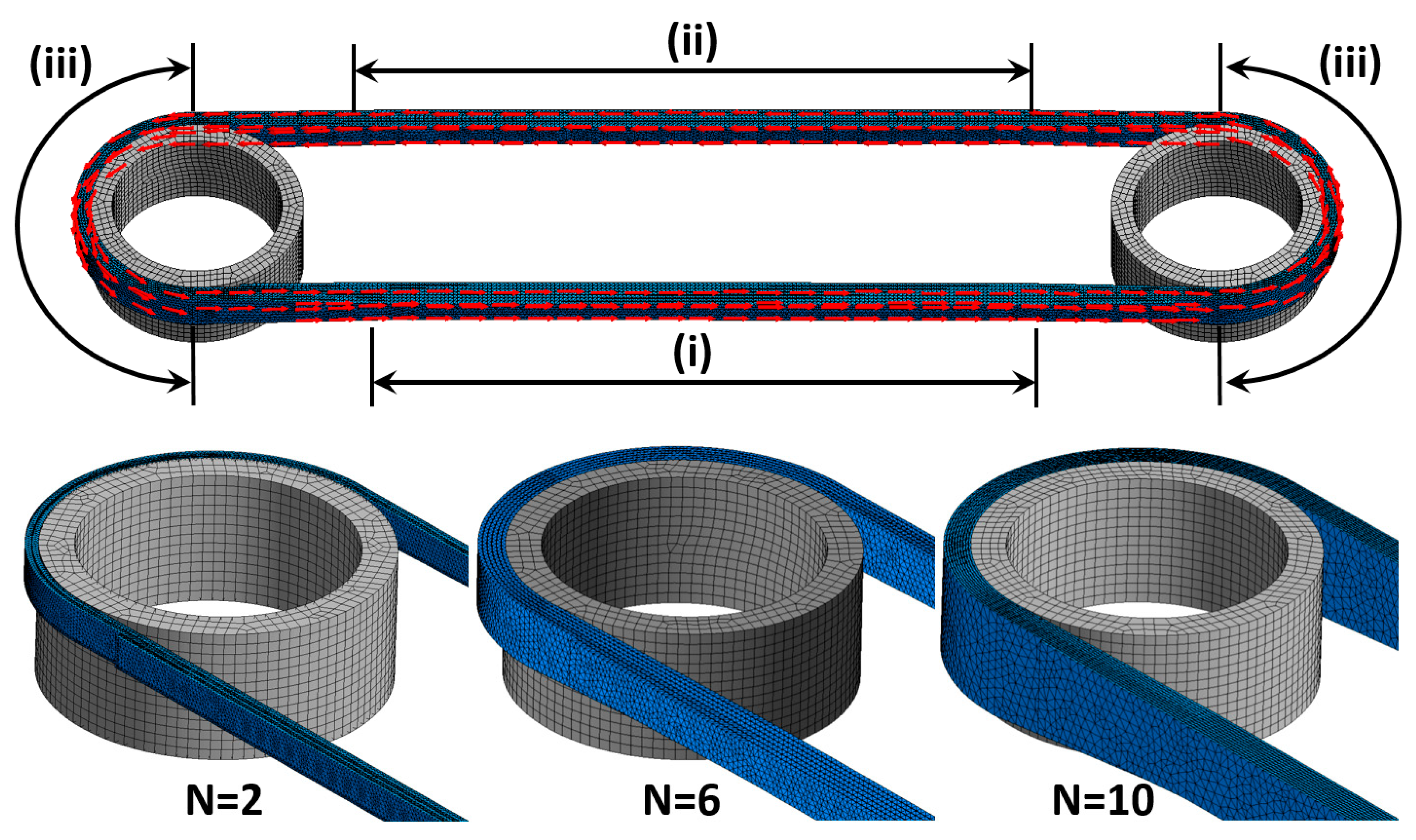
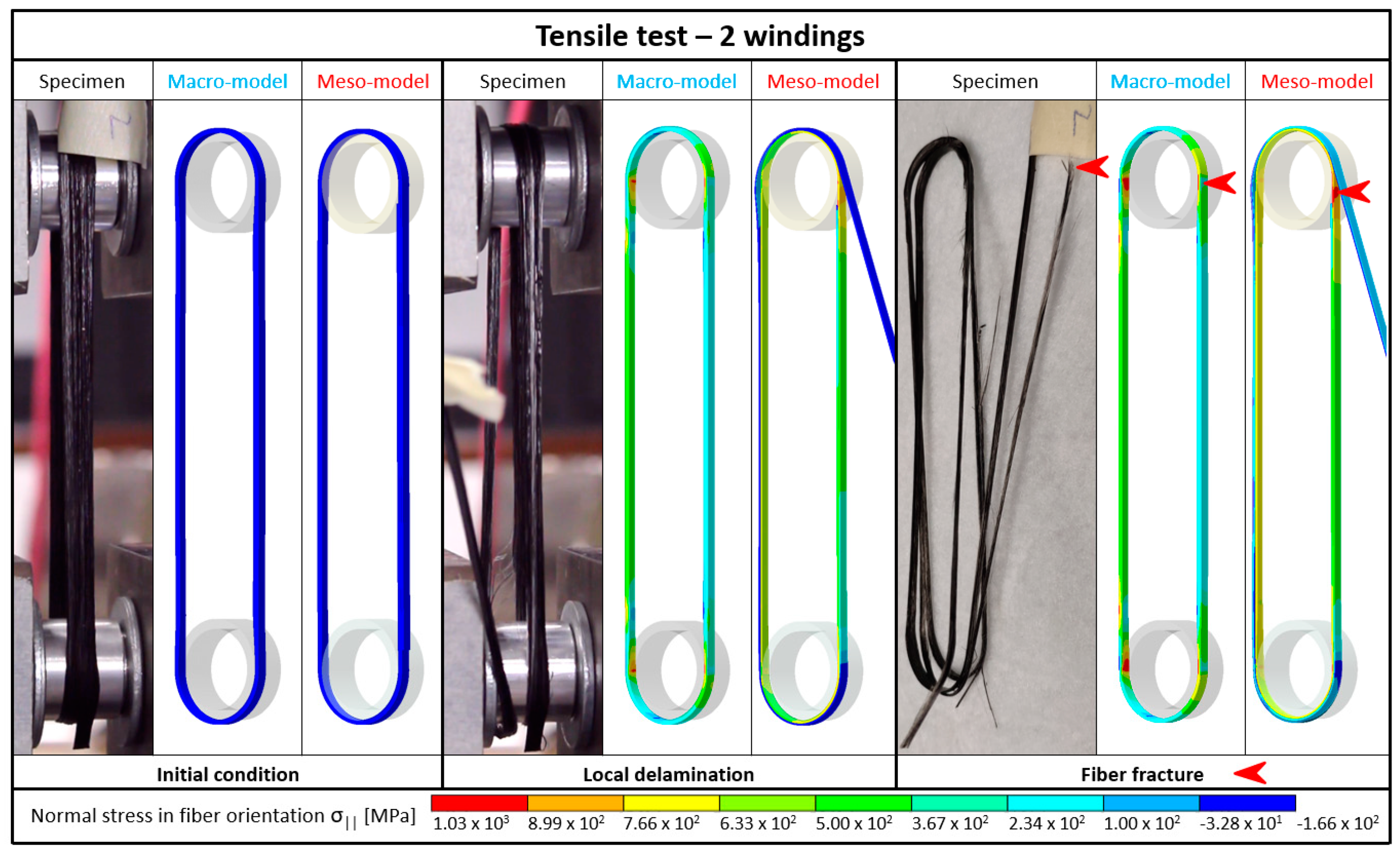
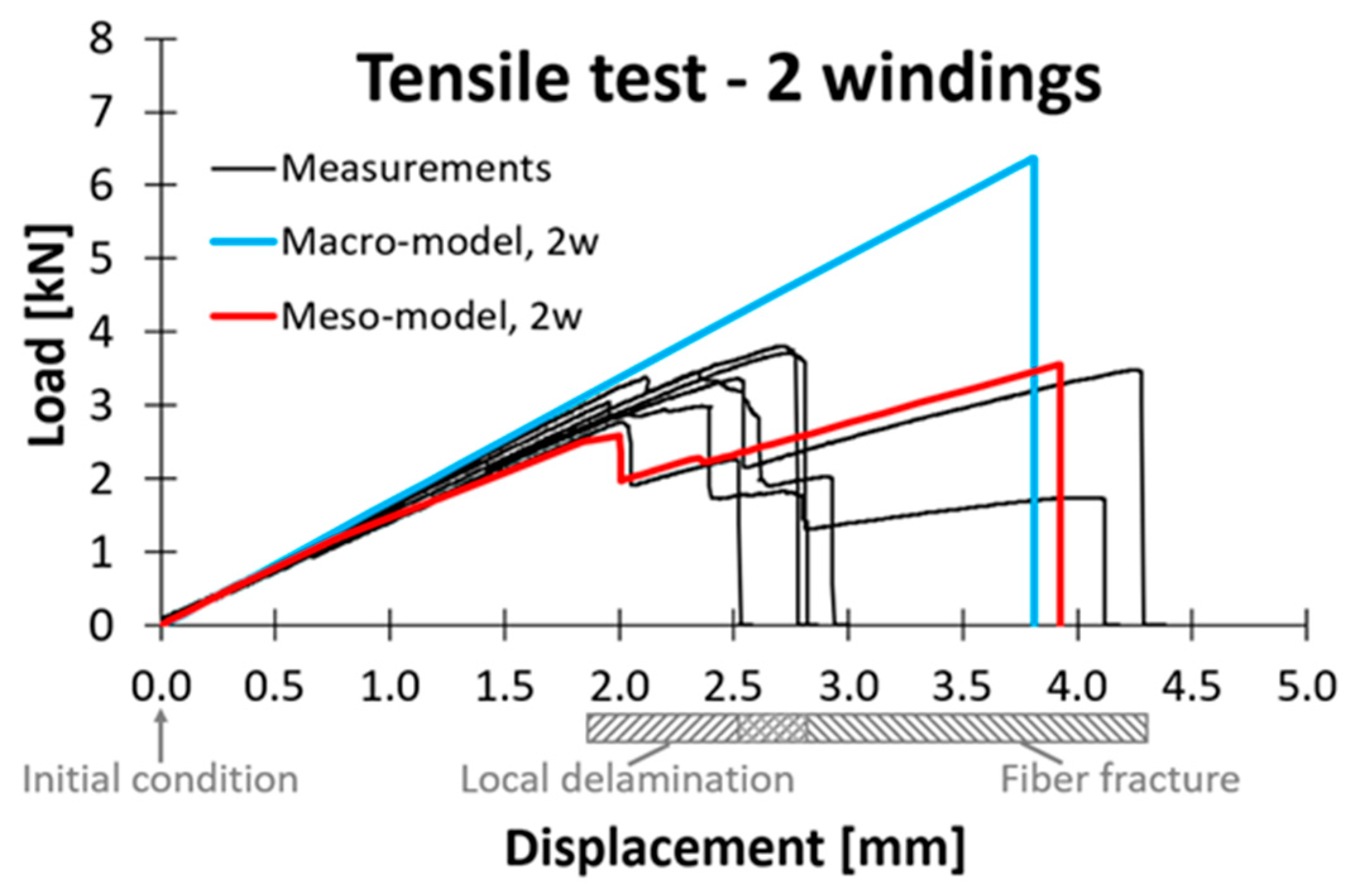
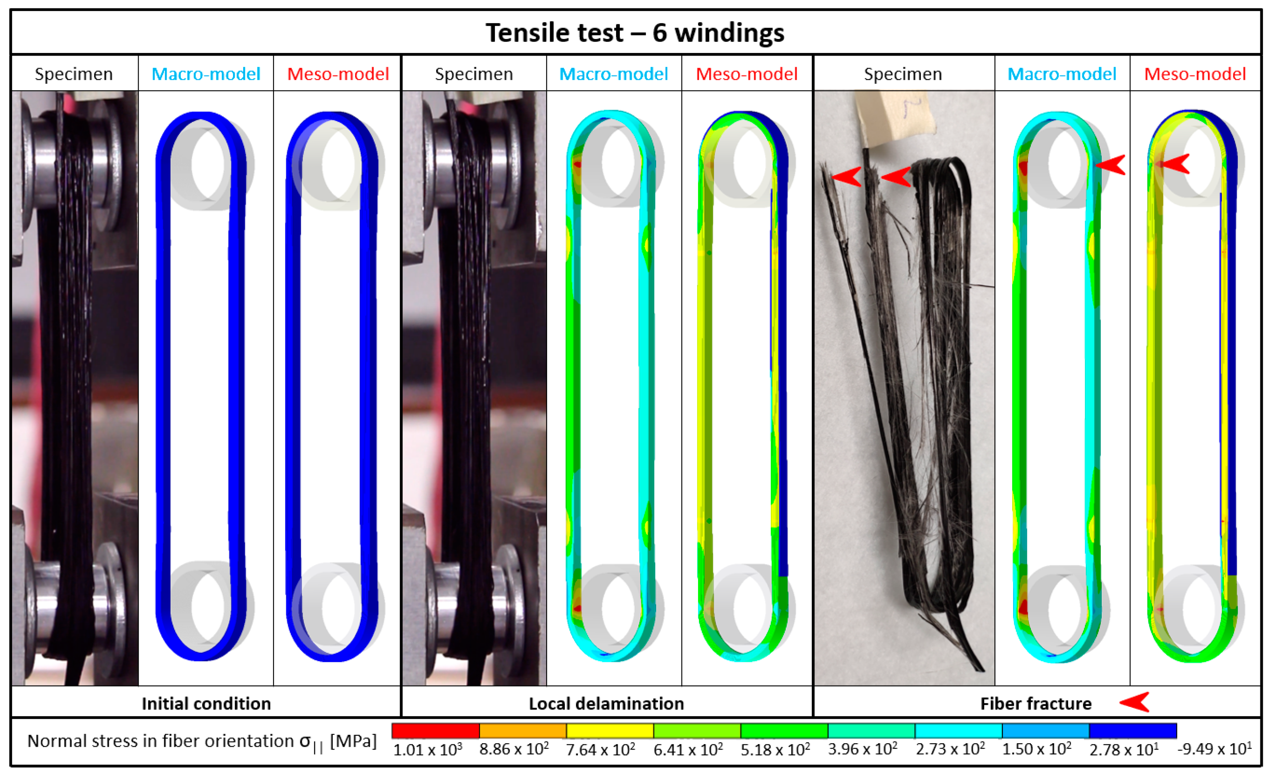
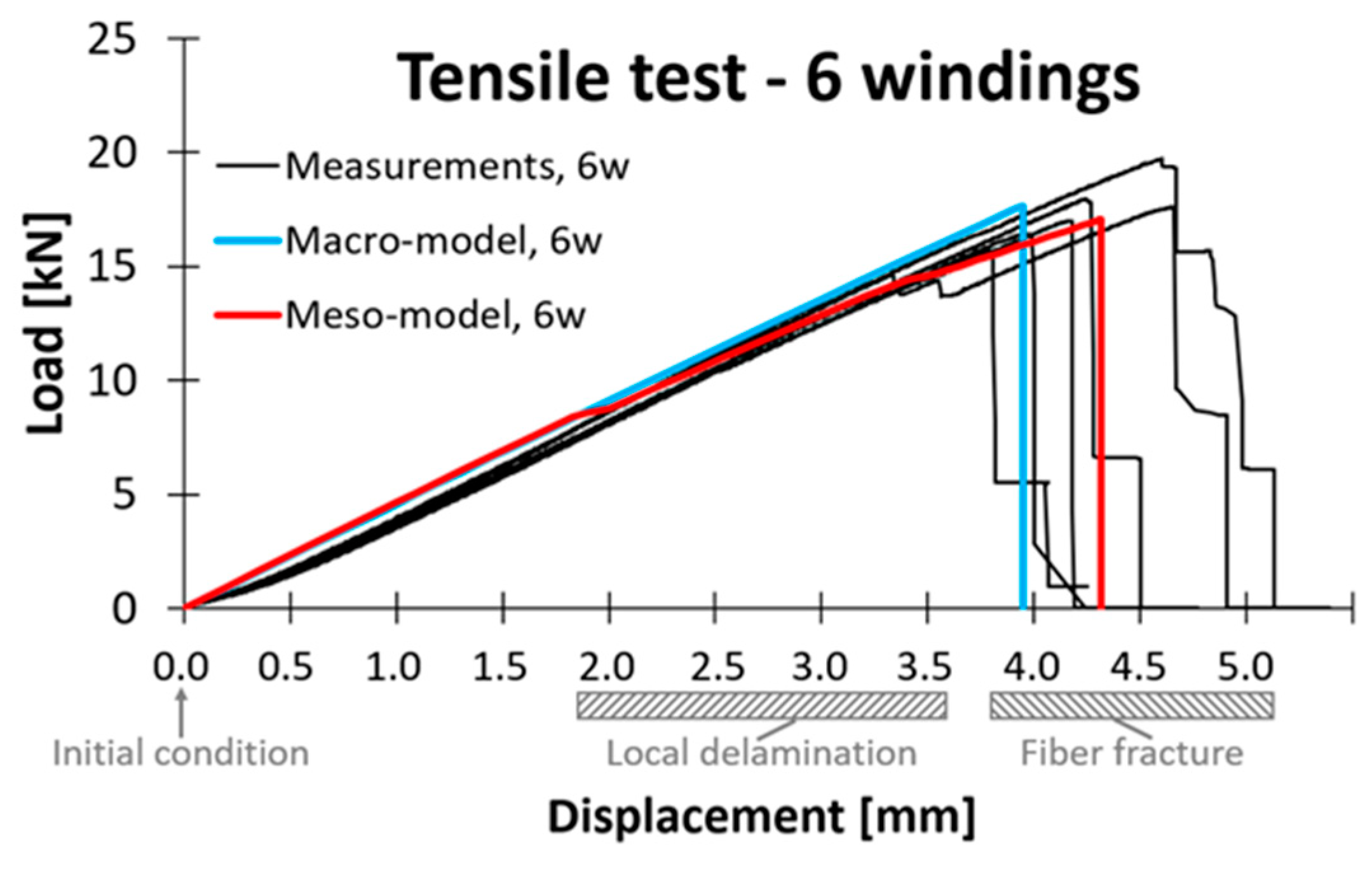
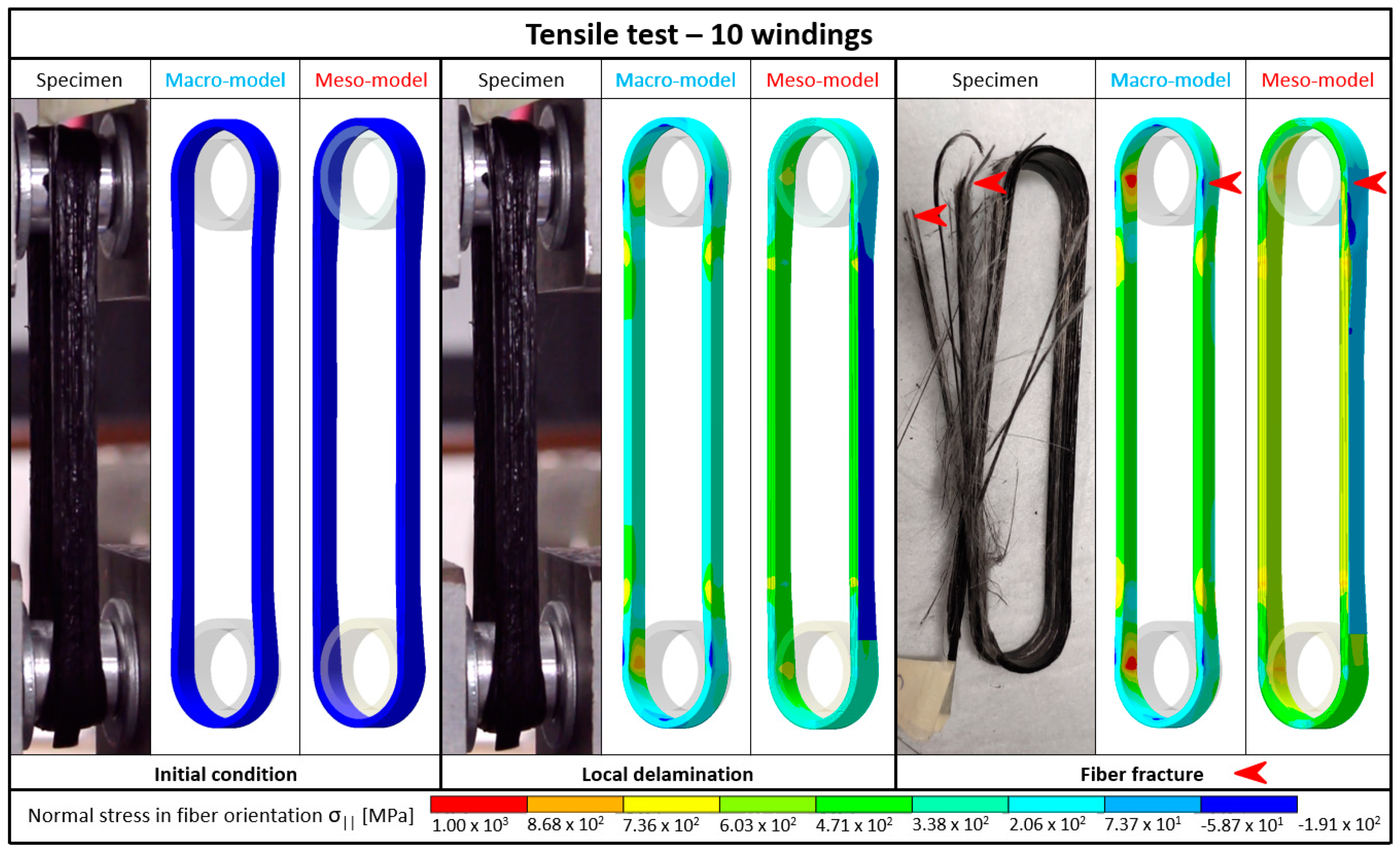
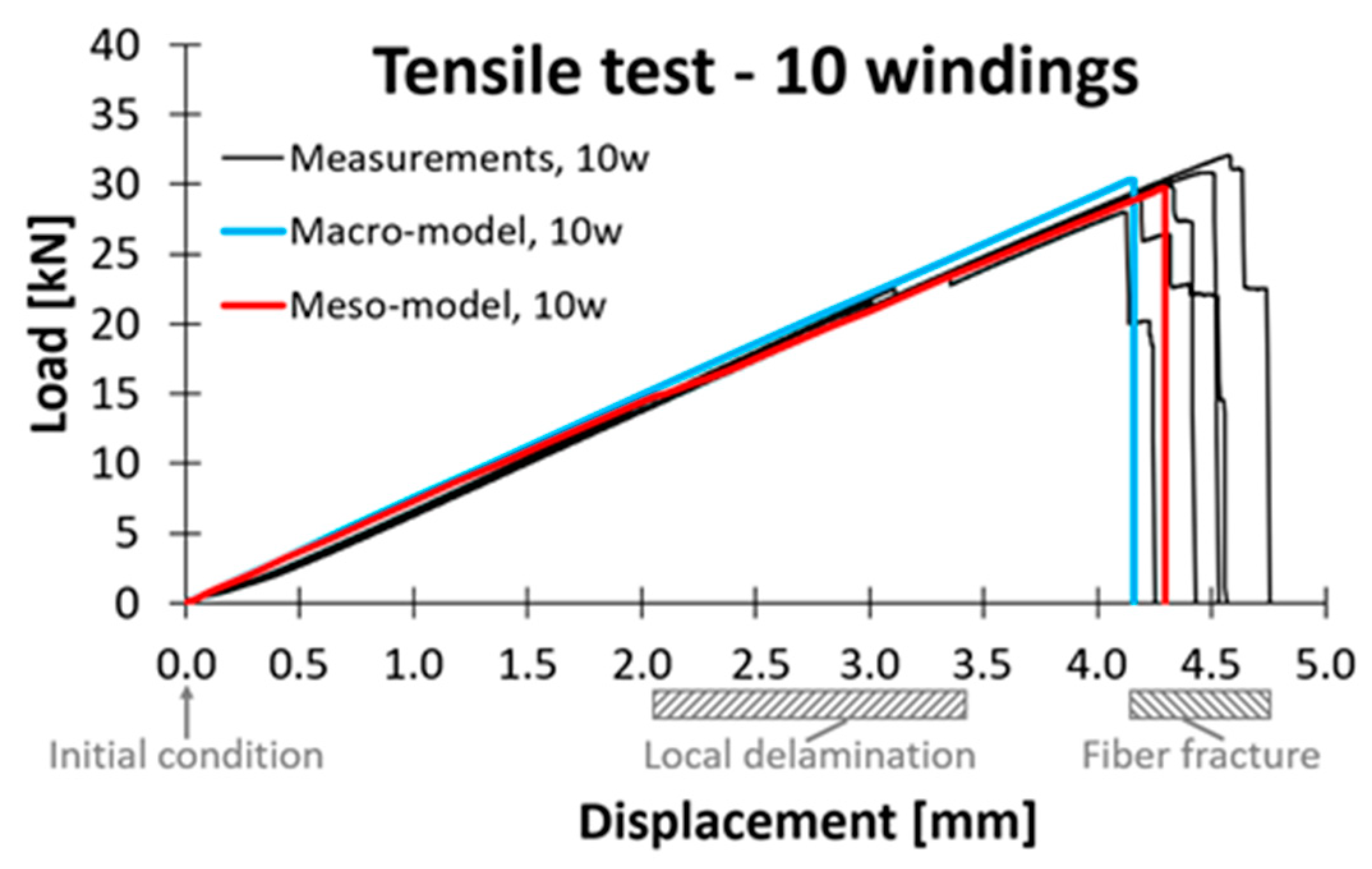
  • It has been shown in [8,21] that delamination has an influence on the mechanical behavior (i.e., the load-displacement curve) of tension-loaded simple loops. However, this influence decreases at higher winding numbers. This indicates that at higher winding numbers, mesoscopic modeling may be abandoned in favor of a time-efficient macroscopic modeling approach (Section 2.2.2), which neglects the roving–roving interface (B). Both modeling approaches are compared using the example of simple loops in this paper (Section 3.2.5).
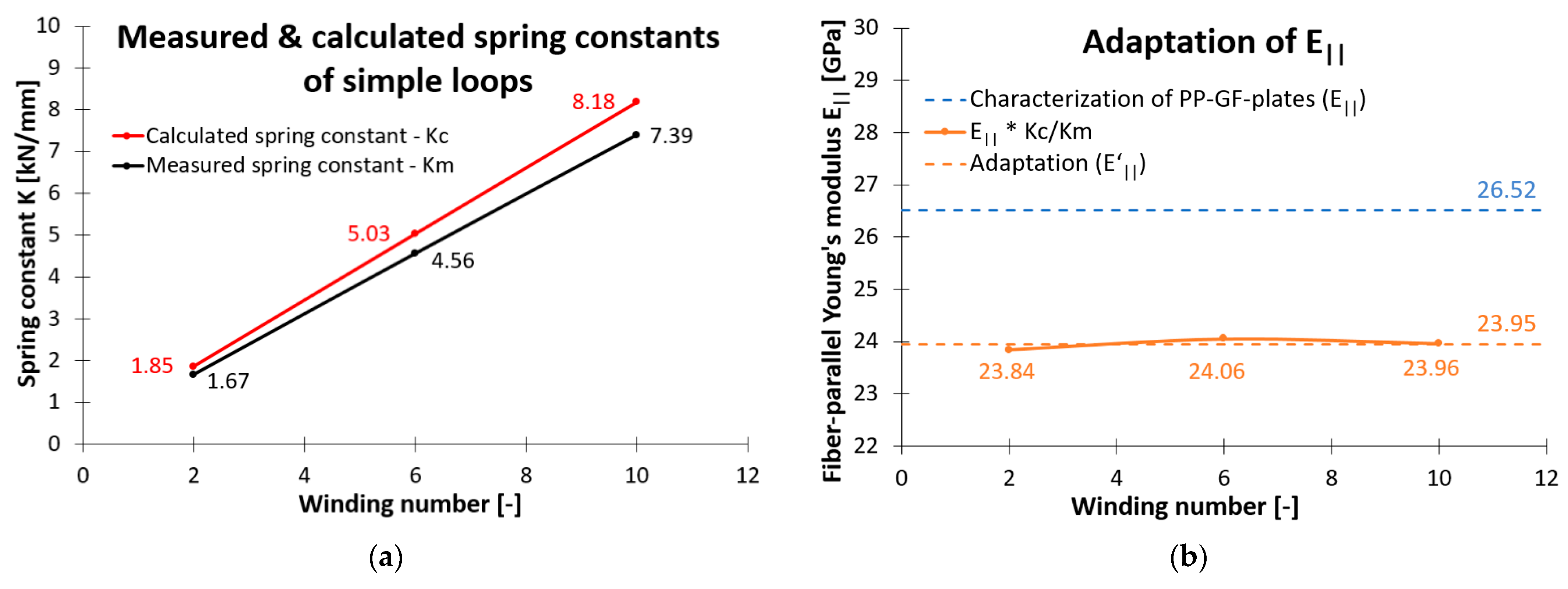
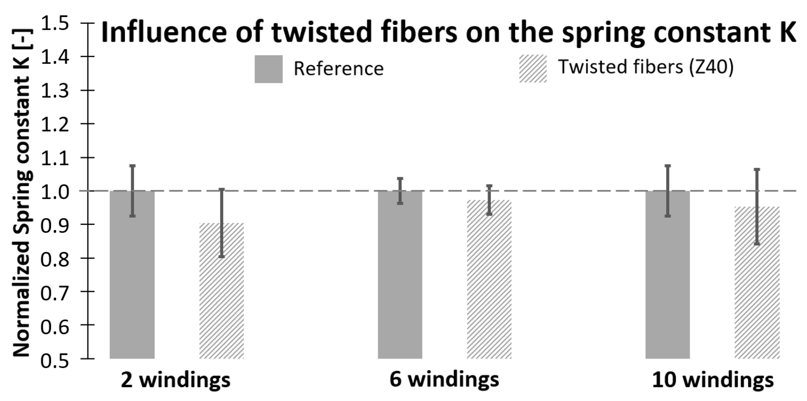
  • The loops’ stiffness measured in N/mm, hereafter referred to as spring constant K , was overestimated in the simulations in [21]. This deviation as well as possible reasons are examined experimentally (Section 3.2.3). Based on the findings, the fiber-parallel Young’s modulus ( E | | ) of the impregnated roving (A) is adapted to the loops’ effective elastic behavior.
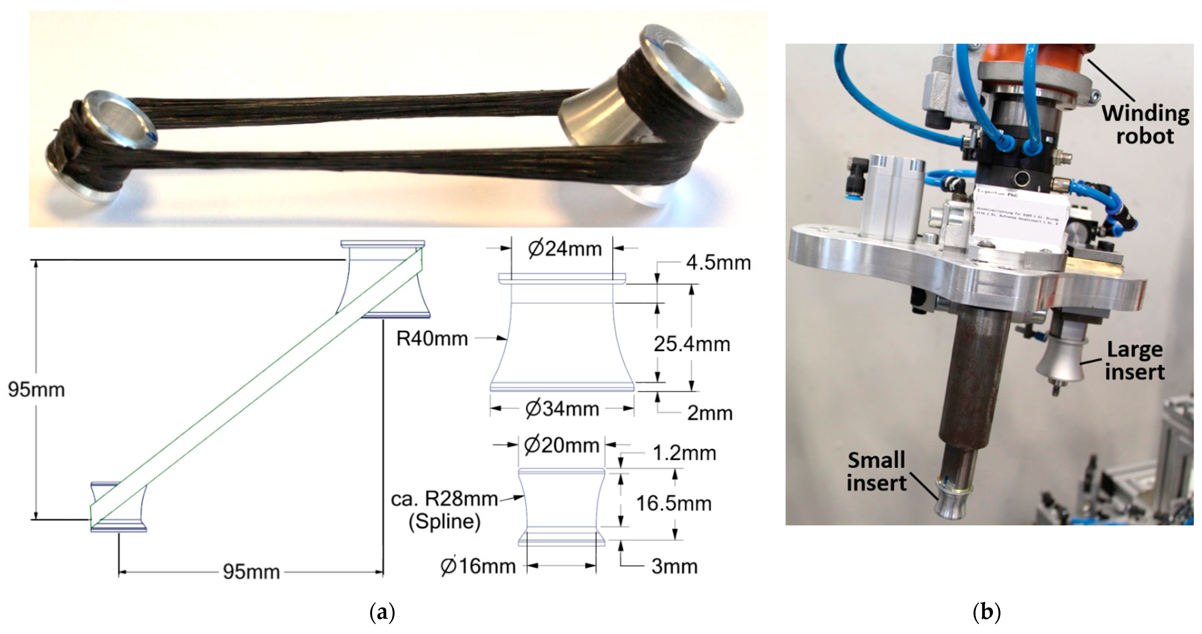
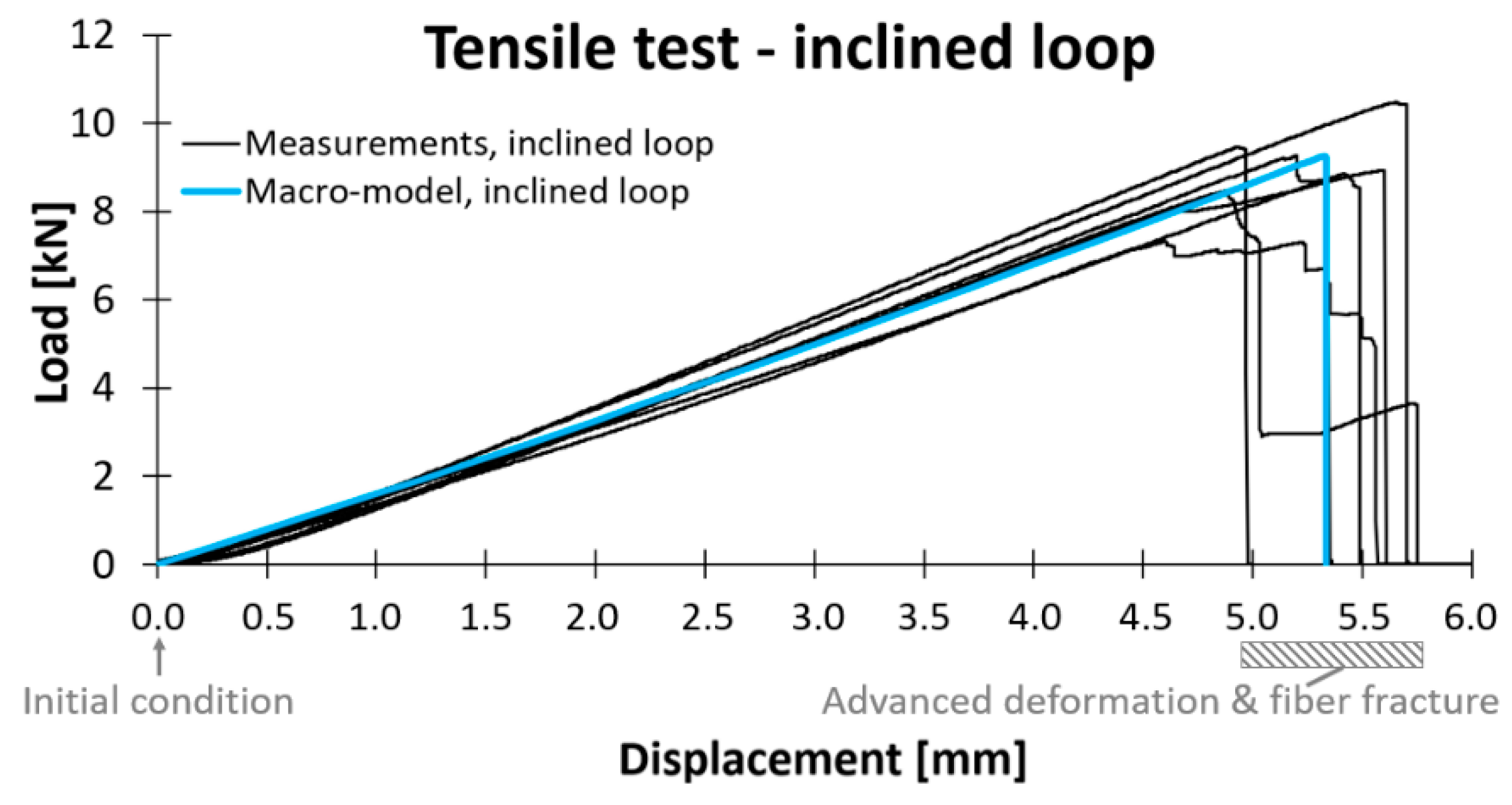
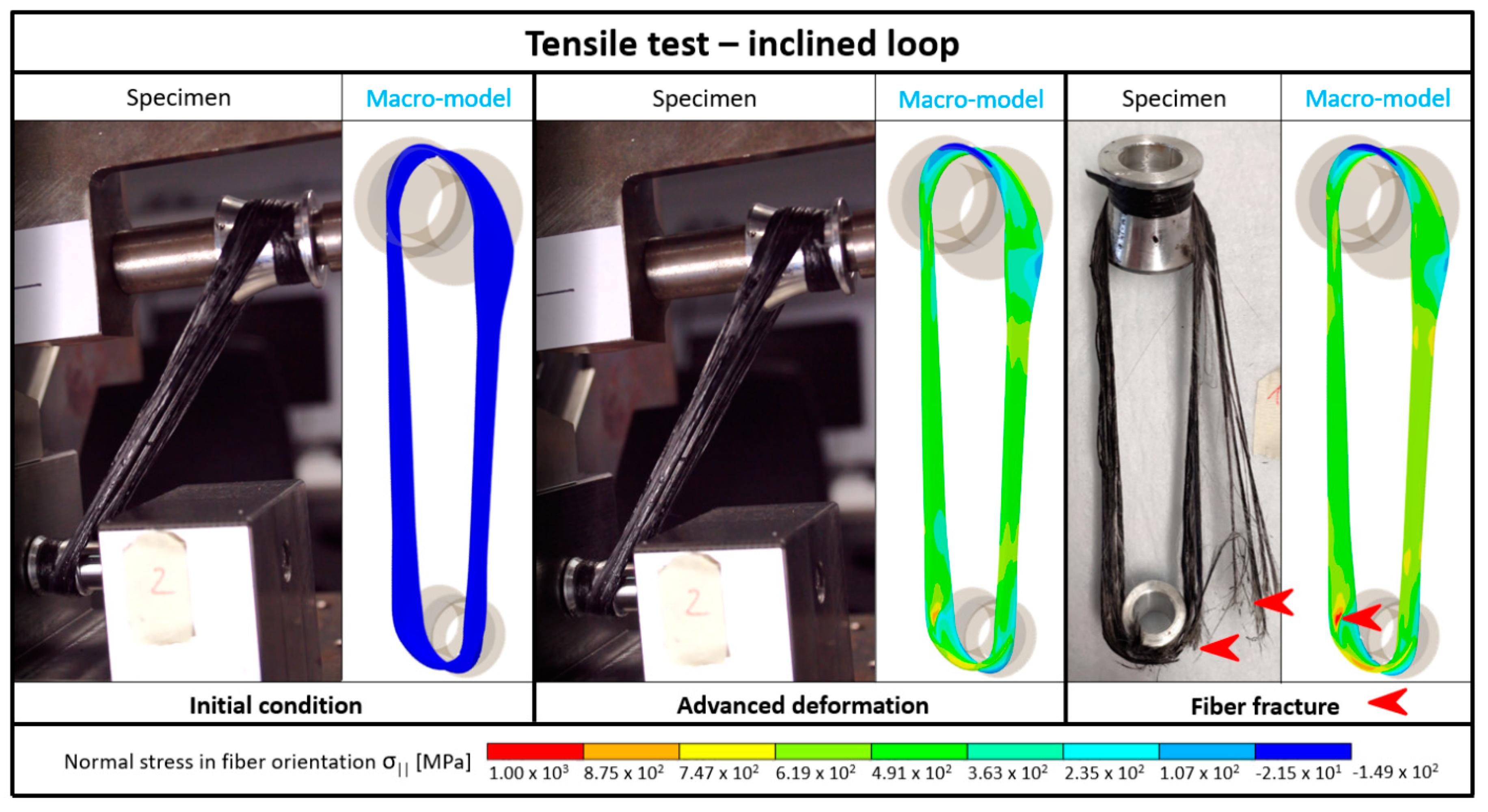
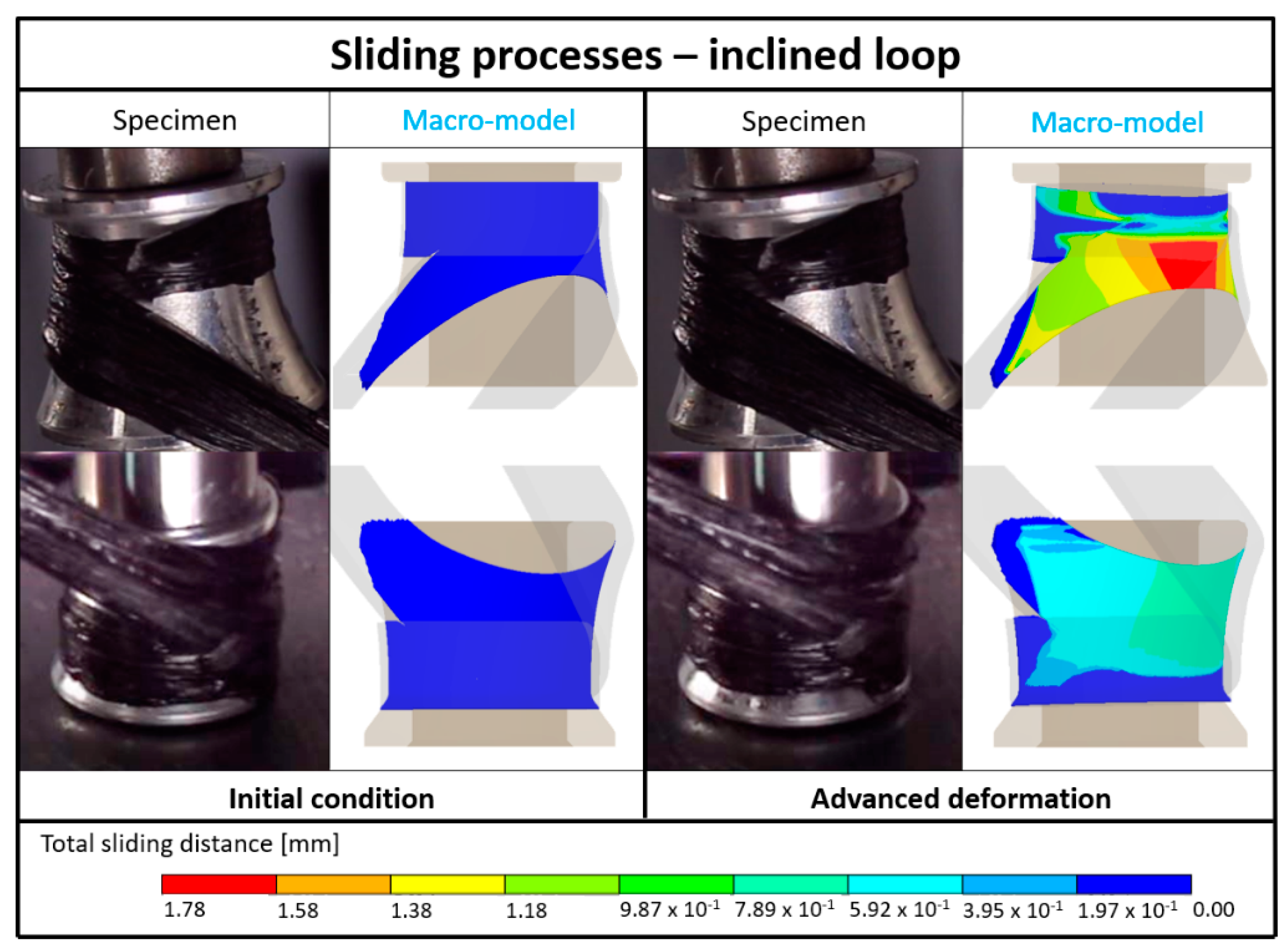
  • After intensive consideration of simple loop structures, the knowledge is transferred to the modeling and simulation of inclined loops and thus to three-dimensional fiber skeletons (Section 3.3). Since relative movements between windings and inserts may occur in this case, the insert-roving interface (C) is characterized in this context (Section 3.1).

2. Materials and Methods

2.1. Specimens and Mechanical Testing

2.1.1. Materials

The materials correspond to the ones used in [21]. All windings as well as the plates for the friction tests are made from the polypropylene-glass fiber (PP-GF) commingled yarn Twintex ® RPP60 1870 B provided by the manufacturer Owens Corning. It has a fiber volume content of 35 vol.-% and a linear density of 1870 tex (g/km). The polypropylene filaments contained in it are colored black. All inserts and the slider for the friction tests are made from aluminum. Table 1 lists the elastic constants and strength values used in the FE simulations.
With two exceptions, the material properties given in Table 1 correspond to the measurements and assumptions from [21]. One exception is the fiber-parallel Young’s modulus ( E | | ) of the PP-GF roving (A) which is adapted in Section 3.2.3 based on the observed deviations between calculated and measured spring constants of simple loops under tensile loading. The other exception concerns the fiber-parallel tensile strength ( R | | t ) which is redetermined in Section 3.2.4. Both adaptations are carried out using FE models of the simple loop and are later validated using an FE model of the inclined loop.
To investigate the influence of fiber twists on the spring constant K of simple loops, a comparable PP-GF commingled yarn with an artificial twist of 40 turns per meter is produced in a cooperation of the companies Comfil ApS (Gjern, Denmark) and Culimeta Textilglas-Technologie GmbH and Co. KG (Bersenbrück, Germany).

2.1.2. Test Specimens

The simple loop specimen, shown in Figure 2, is used in this paper to investigate the influence of different geometric dimensions, to compare meso- and macroscopic geometry modeling and to investigate the spring constant K . The tensile tests on simple loops with two and six windings described in [21] are repeated in this work with optimized production parameters and supplemented by loops with ten windings. In order to investigate a possible cause for the deviation between the calculated and the measured spring constant K , all specimens are additionally produced in a variation with artificially created fiber twist. The production of the simple loop specimens corresponds to the description in [21].
The inclined loop, shown in Figure 3a, is used to investigate more challenging skeleton geometries as well as inclined load transfers typically occurring in three-dimensional fiber skeletons. It is a part of the fiber skeleton developed and investigated in [4]. As the name suggests, the inclined loop differs from the simple loop in that the two inserts are not positioned within the same plane. The specimen considered here shows further differences: the two inserts are of different size, are concave in shape and both completely wrapped twice (double-eye winding on each insert). This configuration originates from the investigations on fiber skeletons with inclined load transfers performed in [4] and is not modified in this paper. The production of the inclined loop is also carried out according to the descriptions in [21], but the winding form shown in Figure 3b and an adapted robot program are used. The inclined loop specimen is dimensioned with four windings. As in the case of the simple loop, a final overlap is applied during the winding process, so that the shaft in the front contains four windings while the one in the back contains five windings. A detailed overview of the winding numbers at every location of the specimen is given in Section 2.2.3.
Since significant movement between the windings and the inserts cannot be ruled out in the case of the inclined loop, the insert-roving interface (C) is characterized experimentally in this work. It is known from previous studies that no significant adhesion occurs between thermoplastic impregnated windings and metallic inserts (especially when using polypropylene matrices), so this contact is considered to be frictional. Consequently, the characterization is based on the DIN EN ISO 8295 standard [28] for the determination of friction coefficients. As can be seen in Figure 4c, plate specimens are used for this purpose which are press-consolidated from the material of the windings and afterwards cut according to standard dimensions. The standard slider, which slides over the plates in the friction test, is made of the material of the inserts (aluminum).

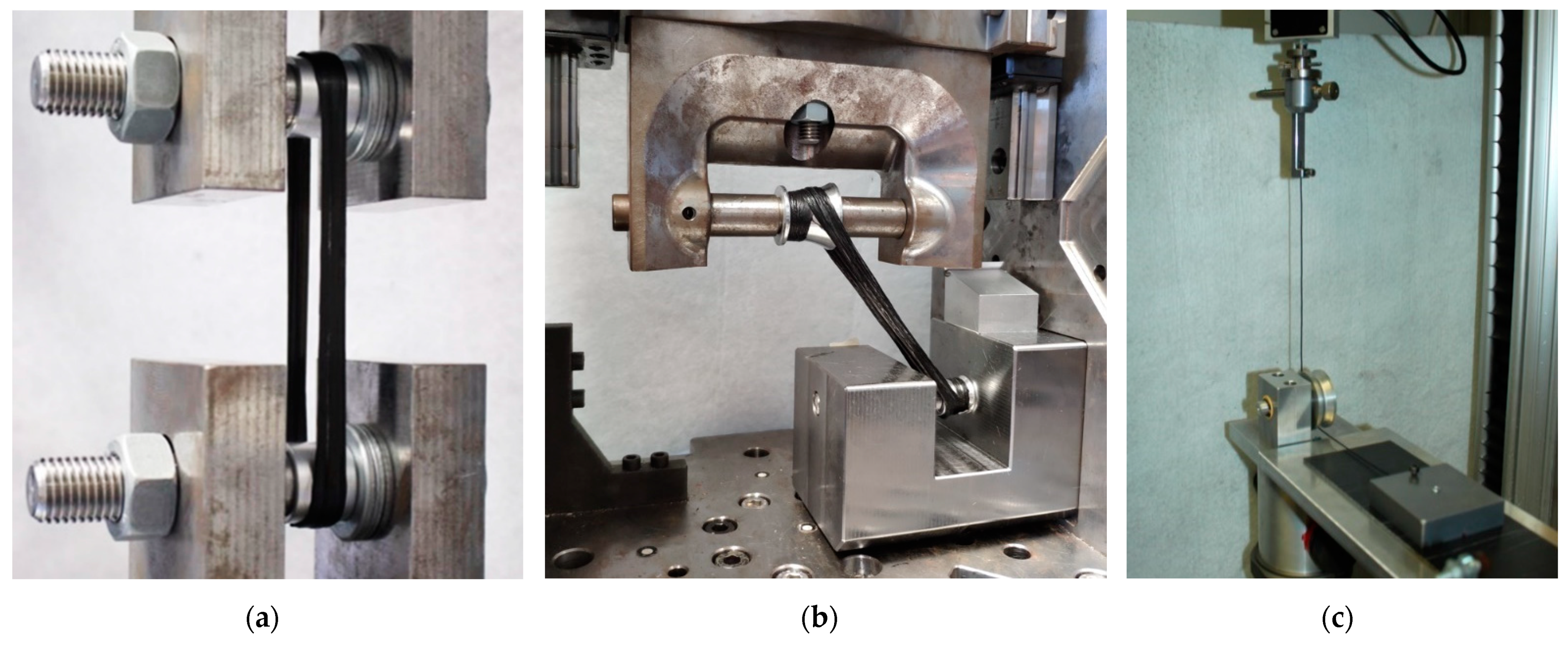
2.1.3. Test Equipment and Procedures

As indicated in Section 2.1.2, tensile tests are performed on simple loops with two, six and ten windings as well as on inclined loops with four windings. As in [21], these are carried out at a testing speed of 5 mm/min on a Hegewald and Peschke inspect table 50 testing machine equipped with a 50 kN load cell and a video extensometer. The corresponding test setups are shown in Figure 4a,b. In both cases, the bottom insert is fixed while the top insert is pulled vertically upwards. The friction tests are performed on a Hegewald and Peschke inspect table 5 testing machine equipped with a 10 N load cell following the DIN EN ISO 8295 standard [28]. The illustration of the test setup in Figure 4c shows that the aluminum slider (200.05 g) is connected to the load cell by a rope. The rope is deflected by about 90° by a pulley so that the slider can slide over the horizontally oriented composite plate. For an approximate estimation of the friction influence of the pulley, additional idle tests are carried out in which the rope is connected only to the pulley. The test speed is set to 100 mm/min in all friction tests. The friction is measured in parallel and transverse to the fiber orientation in the plate specimens.

2.2. Finite Element Modeling

All FE models in this paper are prepared, computed and analyzed with the commercial FE software Ansys Mechanical 2020 R1.

2.2.1. Material Modeling

The material models described and used for the structural constituents (A), (B) and (D) in [21] are adopted in this paper. To represent potential friction effects in the insert-roving interface (C), the basic Coulomb friction model implemented in ANSYS Mechanical [29] is added. Its central relation is given in Equation (1):
τ lim = μ P + b .
τ lim   represents the limit frictional stress, while μ and P are the coefficient of friction and the normal pressure acting between the contact partners, respectively. b represents a contact cohesion providing sliding resistance even without normal pressure. It is set to zero in this work, as no adhesion between inserts and windings is observed.
If the frictional stress of a contact is below the calculated τ lim , the contact partners adhere to each other (sticking state). If, however, τ lim is exceeded, larger tangential displacements between the contact partners are tolerated while the frictional stress remains constant (sliding state). In this simplified model, no distinction is made between static and dynamic coefficients of friction. The resulting relation between frictional stress ( τ ) and tangential displacement ( δ ) is shown in Figure 5. τ is determined by a penalty stiffness, so that very small displacements δ are assumed in the sticking state of a contact [30].

2.2.2. FE Modeling of the Tensile Tests on Simple Loops

As described in Section 2.1.2, much of the research in this paper is done using simple loop specimens as examples. For this type of specimen, two different FE model types are generated whose main difference lies in the geometry modeling: meso-level models in which each winding is modeled individually and macro-level models in which all windings are combined, so that the roving–roving interface (B) is neglected.

Meso-Modeling

The generation of the meso-models is carried out as described in [21] with minor modifications. A detailed description of the modeling is therefore not repeated here. Instead, the changes made compared to [21] are listed below.
  • In [21], discrepancies between simulation results and measurements, as well as uncertainties associated with material characterization, are found. In Section 3.2.3 and Section 3.2.4 of the present work, potential causes are investigated and the material parameters E | | and R | | t of the PP-GF roving (A) are adapted by means of reduction factors. The resulting values are given in Table 1.
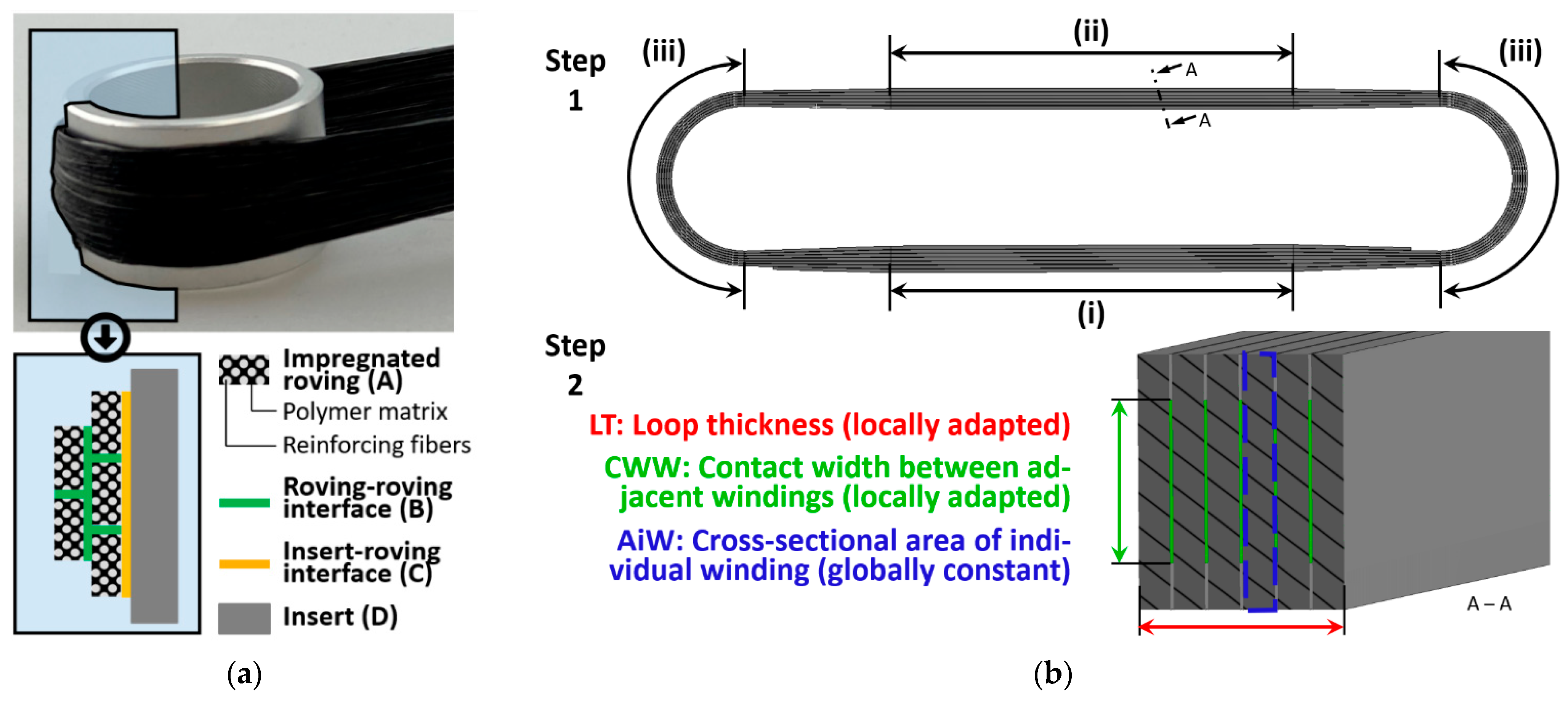
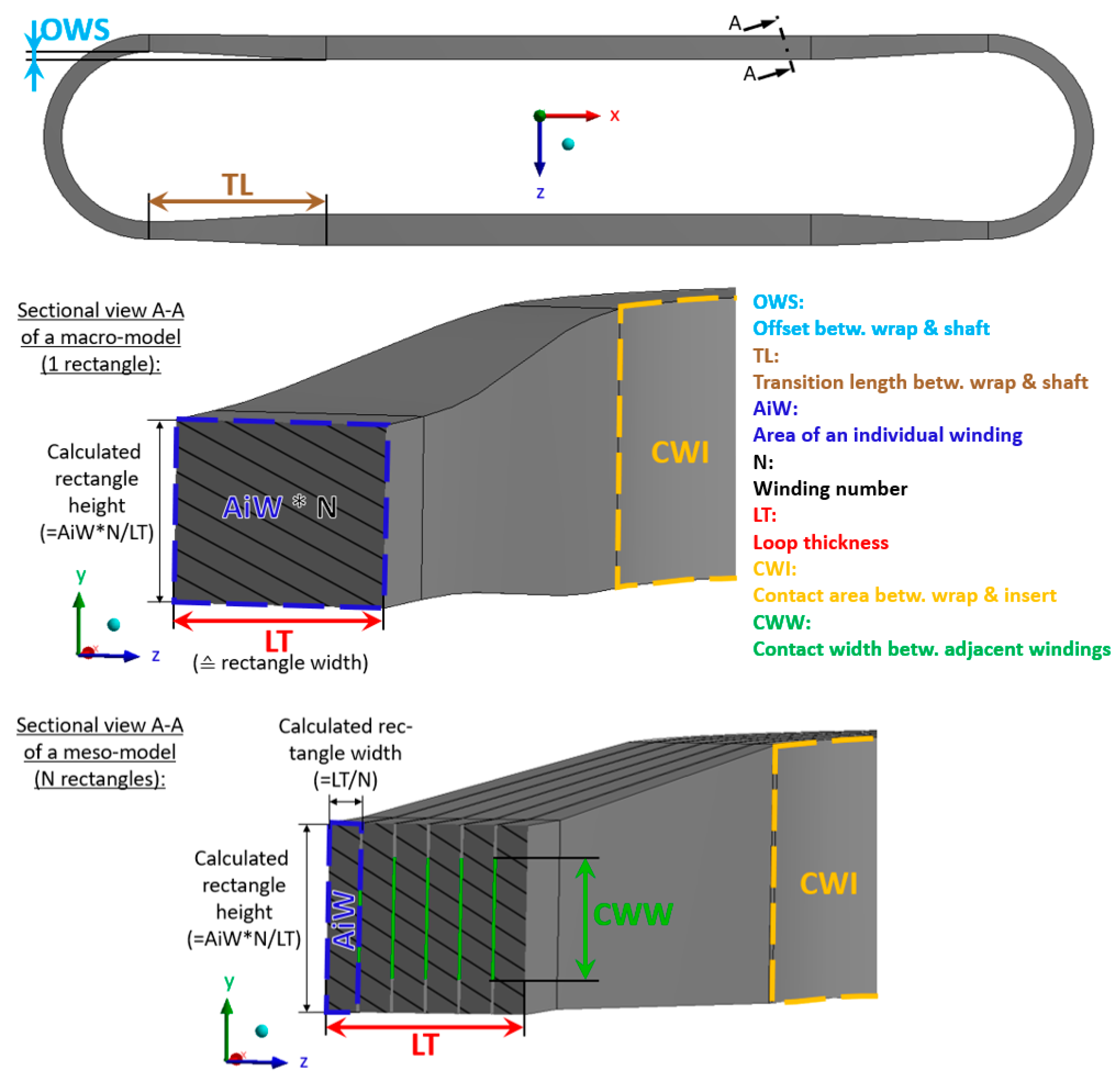
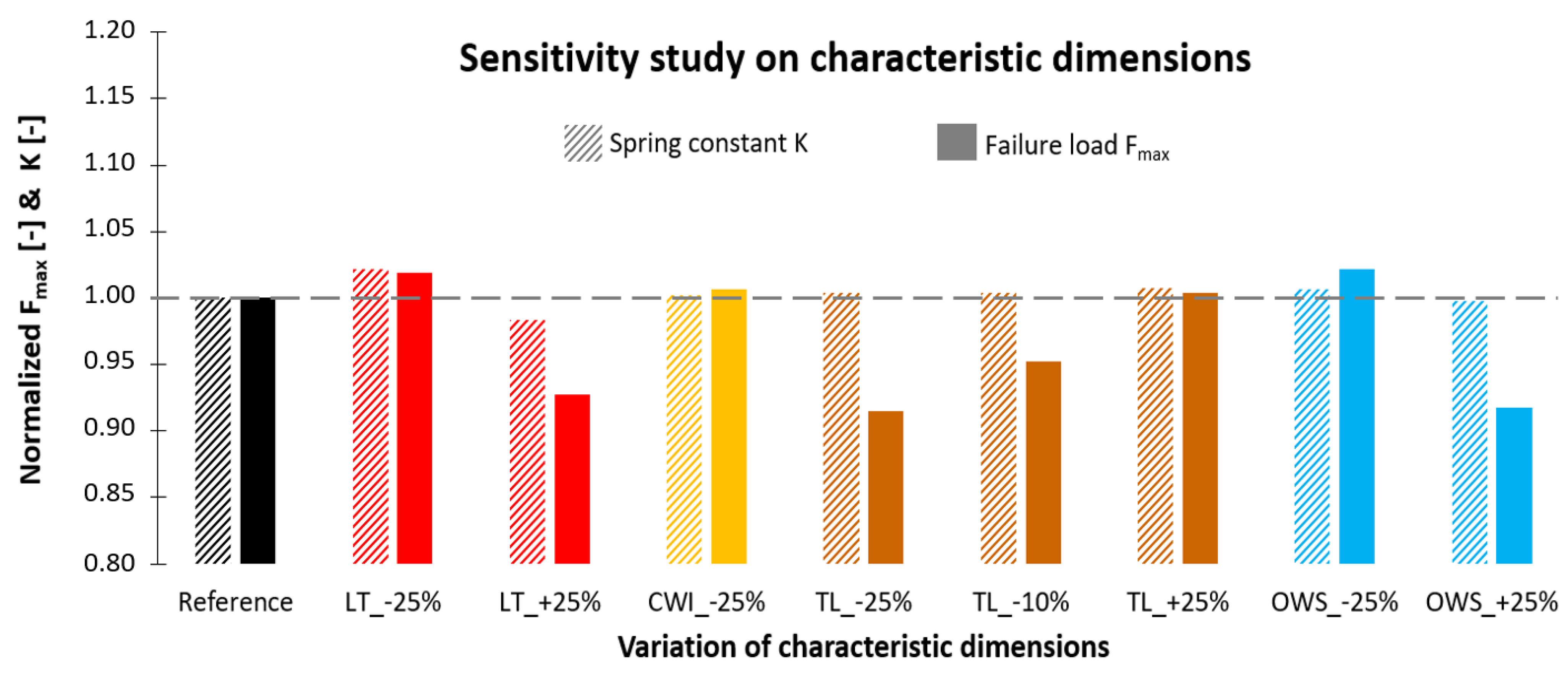
  • As shown in Figure 6, further characteristic dimensions are considered and modeled according to the respective measurements given in Table 2. Their mechanical influence—and thus their relevance for precise FE simulations of fiber skeletons—is evaluated in Section 3.2.2.
  • To reduce calculation time, the symmetric geometry model is halved.
  • Since meshing complex skeleton models with hexahedral SOLID186 elements often leads to poor element quality, all models studied are consistently meshed with tetrahedral SOLID187 elements. SOLID187 is a 10-node 3D solid element with a quadratic shape function and three degrees of freedom per node (x, y and z direction).
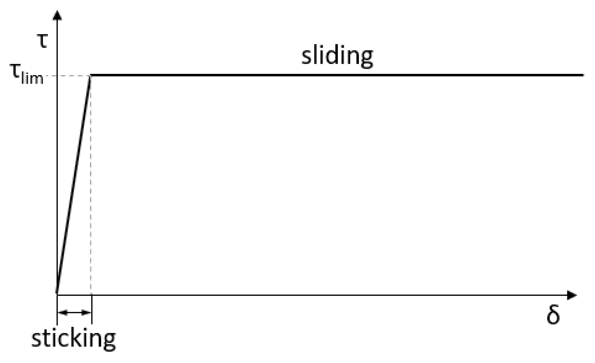
  • The insert–roving interface (C) is no longer represented by a frictionless contact, but by the friction model described in Section 2.2.1 in combination with the coefficient of friction μ S determined in Section 3.1.
  • Geometric non-linearity is considered by activating the corresponding analysis setting in ANSYS Mechanical (“large deflection”). This ensures that deformation-induced changes of the stiffness matrix are determined and adjusted iteratively [31]. Even though the simple loop specimens deformed by only a few millimeters before total failure, the assumption of geometric linearity can lead to unrealistic deformations and stress peaks in the FE simulations. This applies in particular in the context of delamination.
The resulting meso-models are shown in Figure 7. Table 2 lists the characteristic dimensions of the simple loop specimens. The loop thickness (LT) and the contact width between adjacent windings (CWW) are determined based on micrographs as described in [21] with the difference that metal foil is used instead of polyimide foil to enable a more precise measurement of the roving–roving-interface (B). The calculated rectangle height is larger than the measured CWW, which is why special surfaces are defined to model the contact between the windings (marked in green). In addition, 2D images of the loops are made with an optical scanner, from which the offset between wrap and shaft (OWS) and the transition length between wrap and shaft (TL) are measured using the public domain image processing software ImageJ. The area of an individual winding (AiW) is adopted from [21] and the contact area between wrap and insert (CWI) results from the rectangle height in area (iii).
Figure 6. Overview of the characteristic dimensions considered in this work and illustration of the windings’ rectangular modeling.
Jcs 06 00098 g006

Macro-Modeling

To ensure comparability, macro-modeling of the simple loops is based as closely as possible on the meso-models described above. The characteristic areas shown in Figure 7 and the characteristic dimensions specified in Table 2 apply in the same way. The windings are modeled with a rectangular cross-section as well. In contrast to the meso-models, however, there is only one rectangular cross-section per characteristic area, since the interfaces between the windings are neglected. The local cross-sectional area corresponds to the cross-sectional area of an individual winding (2.47 mm2) multiplied by the number of locally present windings. With this value and the local loop thickness given in Table 2 (corresponds to the width of the rectangle), the local height of the loop (height of the rectangle) results are unambiguous. This is graphically explained with the characteristic dimensions in Figure 6. Another difference between the meso- and macro-models concerns the transitions between the shafts (i, ii) and the wraps (iii). In the meso-models, these must be modeled as straight-line connections to maintain close contact between the adjacent windings. Due to the neglection of the roving-roving interface (B), this restriction does not apply to the macro-models, so that the notches associated with straight-line modeling can be avoided here. Therefore, the transitions are modeled based on curves, in this case, which tangentially fade into the shafts and wraps (see Figure 6). This also leads to a more realistic representation of the fiber skeletons’ actual shape. As with the meso-models, the material properties specified in Table 1 are used and aligned with the (idealized) fiber orientation by adjusting the elements’ local coordinate system. The insert–roving interface (C) and all analysis settings are also defined identically. Furthermore, the macro-level geometry models are also meshed with tetrahedral SOLID187 elements, and the load introduction is also carried out by displacing one insert while the other one is fixed.

2.2.3. FE Modeling of the Tensile Tests on Inclined Loops

From past studies it is known that delamination is unlikely to occur in wound loop structures with eye windings. For this reason, geometry modeling on the meso-level is skipped and a macro-model of the inclined loop specimen is generated instead. As can be seen in Figure 8, in this case as well, the geometry modeling starts with a segmentation of the fiber skeleton into characteristic areas. As with the simple loops, the two shafts (i, ii) are distinguished here, since they contain different winding numbers. The two outer wraps of the inserts (iii, iv) are modeled differently, since the two inserts are not identical. The inner wraps (v, vi) are added as additional characteristic areas to model the eye windings. The shafts and the outer wraps are connected by tangential transitions in this case as well. Again, the modeling of the windings is based on rectangular cross-sections as indicated by the equations shown in Figure 6. This time the measurements of the inclined loop, given in Table 3, are used. The measurement of the inclined loop is carried out using the optical 3D measuring system ATOS 5 provided by GOM GmbH. Thus, as shown in Figure 8, the outer surfaces of the skeleton are comprehensively measured, but no section views are available. Thus, the loop height (height of the rectangle) is measured in this case and the loop thickness is derived from it. This again requires the cross-sectional area of a single winding (2.47 mm2) and the number of locally present windings given in Table 3.
The inclined orientation of the loop and the concave insert designs require more complex geometry modeling than with the simple loop. The key adaptations are listed below:
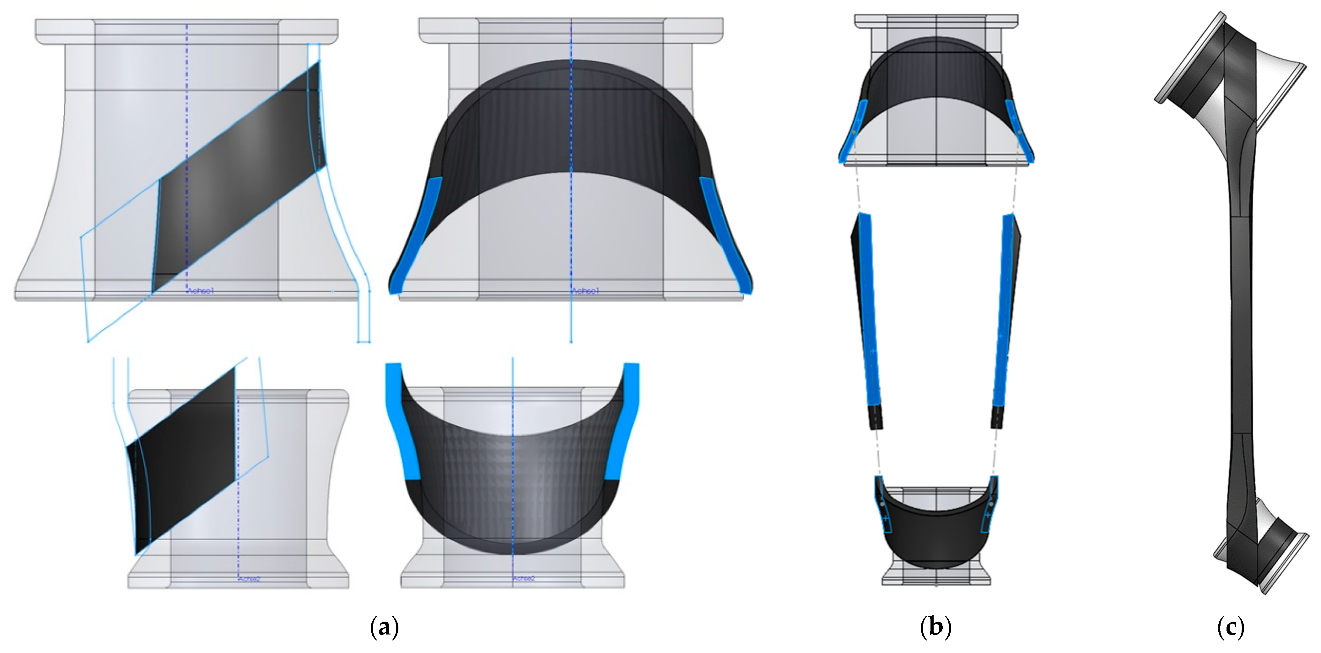
  • As shown in Figure 9a, the cross-sections of the outer wraps follow the insert shapes and are therefore not rectangular but rectangle-like: they have a constant wall thickness and parallel edges; however, two of the four edges are not straight. This modeling approach enables a close contact between insert and windings while keeping implementation simple. The inner wraps are modeled in the same way and are connected to the outer wraps by bonded contacts.
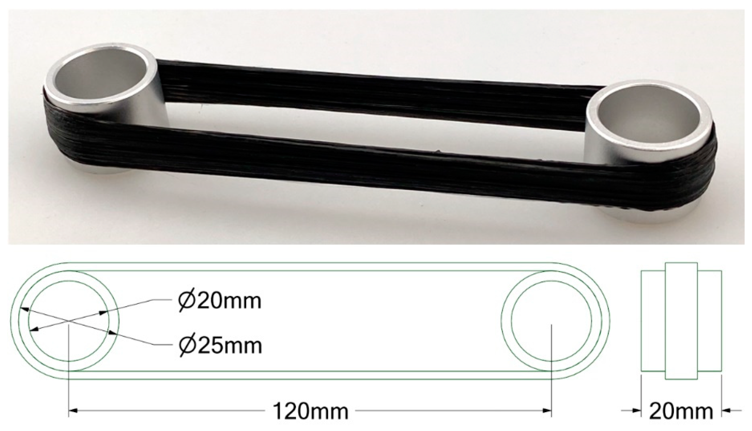
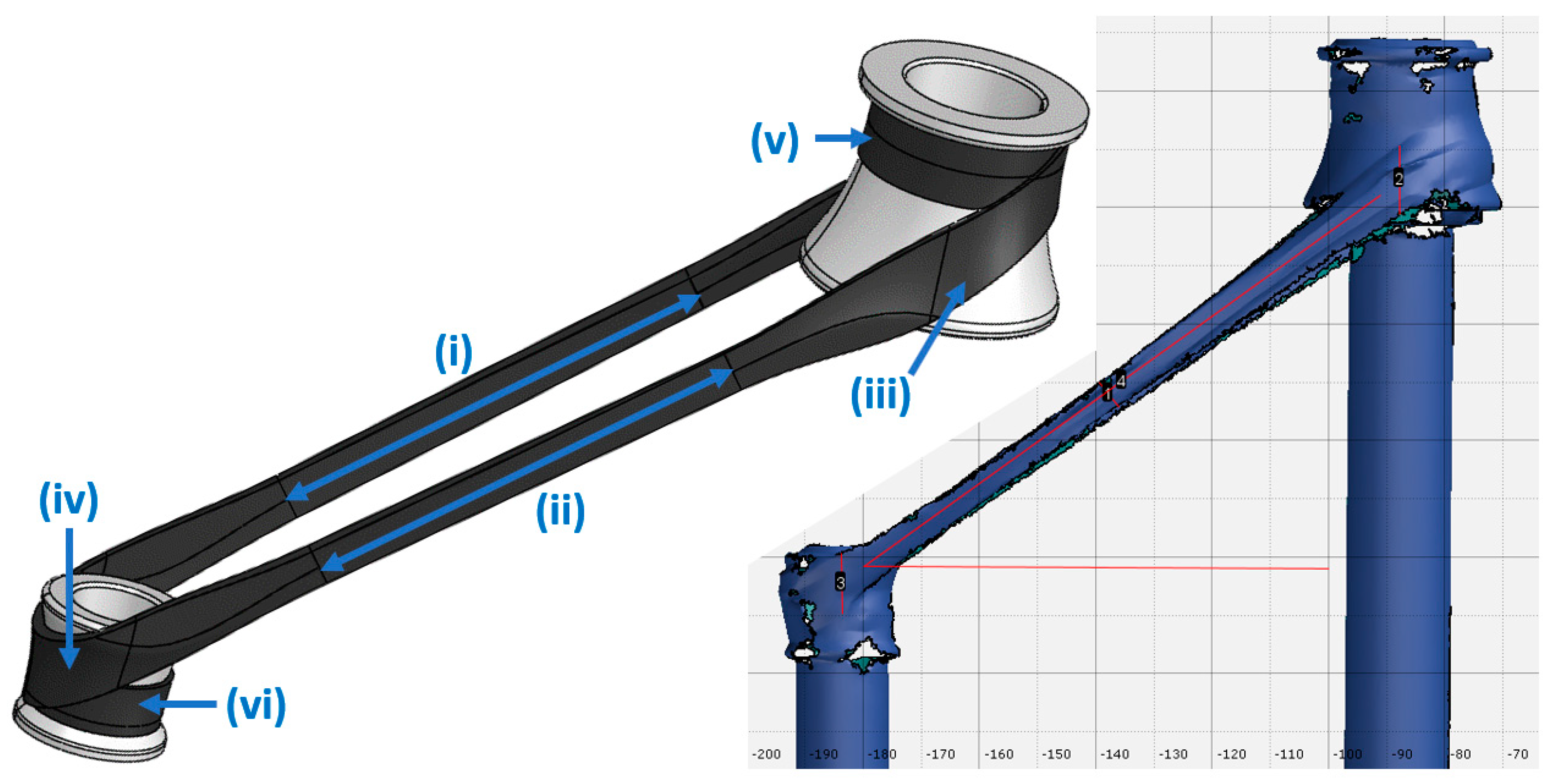
  • The inserts have different diameters. The two outer wraps therefore do not form a semicircle around the inserts (180° deflection), as is the case with the simple loop. Instead, a larger deflection angle is modeled at the large insert and a smaller one at the small insert. This can also be seen in Figure 9a.
  • Analogously to the simple loop, the shafts are modeled with a rectangular cross-section. However, in this case, the shafts are twisted so that their ends match with the angled ends of the outer wraps. The twist of the shafts is shown in Figure 3a (real specimen) and in Figure 9b (geometry model).
  • Due to the twist in the shafts, the OWS and the TL are difficult to measure. The OWS is therefore not considered in the geometry model. Instead, the free shafts are simply centered between the two wrap endings they connect. Based on the recommendations in Section 3.2.2, the TL is set to 25% of the distance between the insert centers.
  • The windings are not aligned perpendicularly to the insert axes, but at an incline to them. As can be seen in Figure 9c it is ensured that the outer wraps and the shafts, as well as the transitions connecting them, are all oriented at a uniform angle. Thus, unrealistic bending moments in the windings are avoided.
The rest of the modeling (material modeling, load introduction, analysis settings) corresponds to the descriptions given in Section 2.2.2.

2.2.4. Geometry, Mesh and Load Step Size Dependencies

To investigate the influence of the different characteristic dimensions shown in Figure 6 on the calculated mechanical behavior of the simple loops, a sensitivity study was performed using a generic macro-model of a simple loop specimen. First, the reference model was generated and subjected to a simulation of a tensile test, as described in Section 2.2.2. Then the characteristic dimensions were in-/decreased individually by +25% and −25%, while ensuring that the cross-sectional area of the windings is identical in all models. The models created in this way were then simulated analogously to the reference model so that the effects of the geometry modification can be seen by direct comparison of the results.
To avoid mesh and load step size dependent results, respective convergence studies are performed prior to the simulations described in Section 2.2. For this purpose, the mentioned reference model is simulated with different mesh and load step resolutions.

3. Results and Discussion

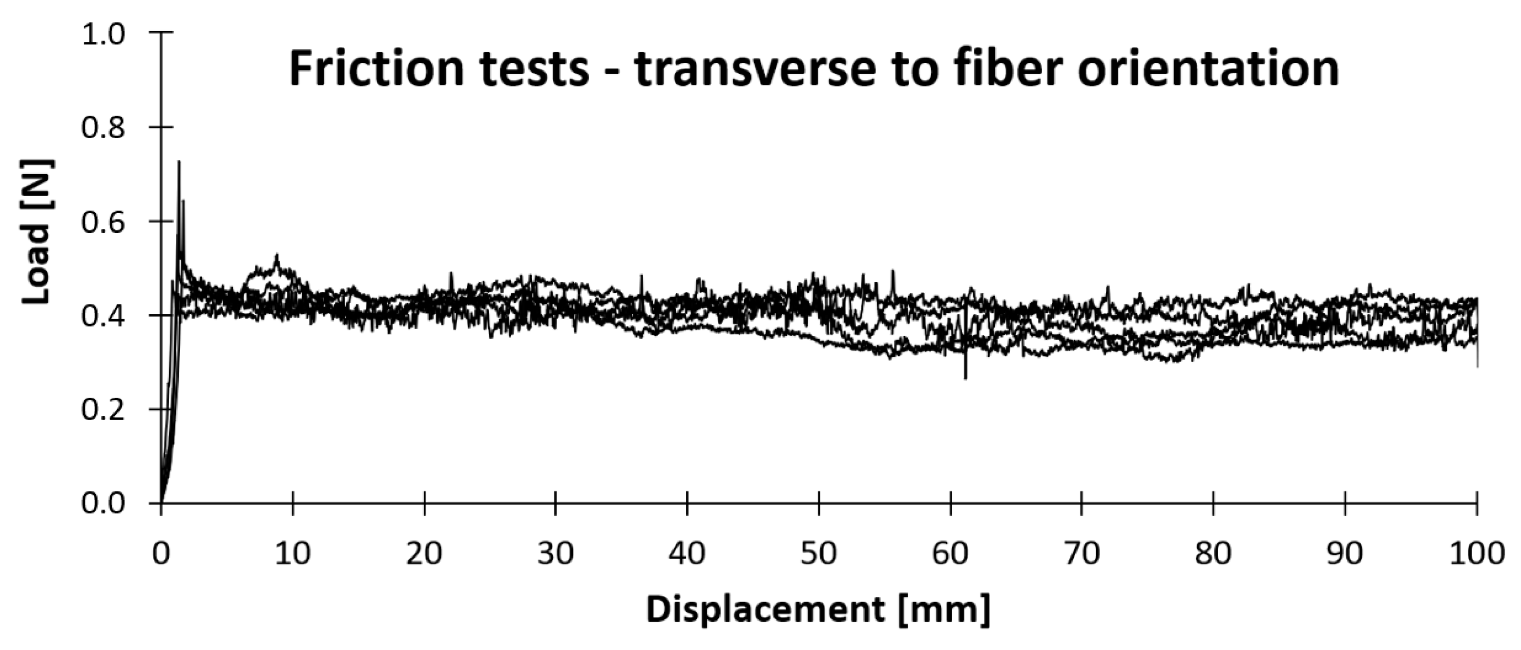
3.1. Characterization of the Insert-Roving Interface (C)

Figure 10 shows some load-displacement measurements of the friction tests used to characterize the insert-roving interface (C). A typical course of friction tests can be seen: it starts with a load peak representing the exceedance of the limit friction stress, then the load settles at a nearly constant level which reflects dynamic sliding.
The static and dynamic coefficients of friction given in Table 4 are determined after Equations (2) and (3), respectively:
μ S = F S F N   ,
μ D = F D F N   .
μ S and μ D represent the static and dynamic friction coefficient while F S and F D are the static and dynamic frictional force. F N represents the weight of the slider.
For F S , the maximum load at the start of the measurement curves is used. F D is defined as the average load measured in the displacement range between 10 and 60 mm. The idle friction load of the pulley is subtracted from both values.
As significant relative movements between windings and inserts are primarily expected transverse to fiber orientation and as the friction model described in Section 2.2.1 only considers static friction, the μ S -value of 0.25 is relevant for this work.

3.2. Investigations on Simple Loop Specimens

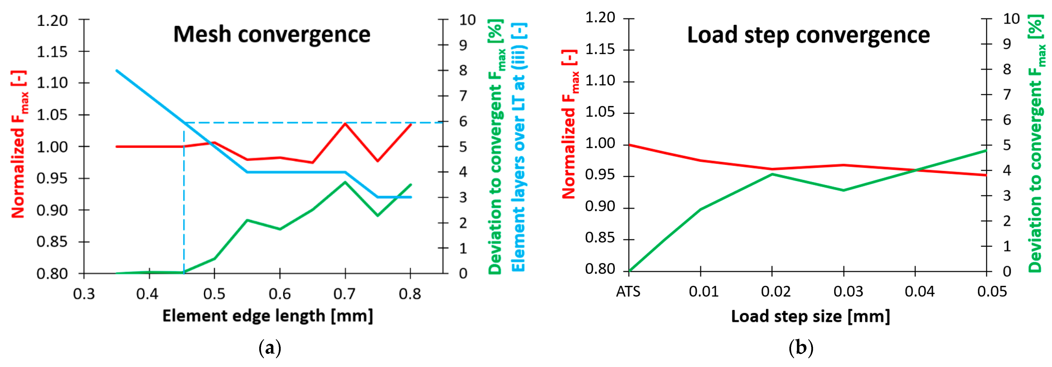
3.2.1. Mesh and Load Step Convergence

As described in Section 2.2.4, a generic macro-model of the simple loop is used to investigate discretization influences on the calculated mechanical behavior. Figure 11a shows the calculated normalized failure load F max as a function of the elements’ edge length (red curve). Besides, the percentage deviation compared to the convergent F max is given (green curve). It can be seen that using an edge length of 0.45 mm or smaller, F max varies less than 0.1%. The third curve indicates the number of element layers over the loop thickness (LT) in area (iii) (blue curve). It seems that a minimum of six layers is required to achieve convergence. This rule is confirmed using other macro-models, while the element edge length required to attain convergence varies between the models. Therefore, all macro-models in this work are meshed with six element layers in the wrap areas.
In a similar way, the influence of the load step size on the calculated mechanical behavior is investigated. Again, the generic macro-model is used as a reference. Non-linear behavior is expected due to fiber fracture (represented by the Maximum Stress Criterion and the MPDG). For its calculation, an implicit iterative solver (Newton-Raphson) and stepwise load application are used. As can be seen in Figure 11b, the precision of the non-linear calculation depends on the resolution of the load steps, which are defined by the displacement of an insert (see Section 2.2.2). As the step size decreases, the calculated F max (red curve) approaches the convergent solution determined using the Automated Time-Stepping feature (ATS) (automatic load adjustment is implemented as automatic time adjustment in ANSYS Mechanical, as loads are generally defined in dependency of time). ATS automatically adjusts the load step size to the current situation of an analysis (e.g., non-linearities) [29]. If necessary, extremely fine load step resolutions are realized. As the deviation from the convergent solution (green curve) indicates, this enables a notable increase in precision here, even compared to fine constant load step sizes. Consequently, all simulations in this work are performed using the ATS feature. It is assumed that it is also suitable for the calculation of non-linearities based on delamination (represented by the CZM in the meso-models).
The mesh convergence study is performed using the ATS feature. The load step convergence is performed using a mesh with six element layers over LT in area (iii).

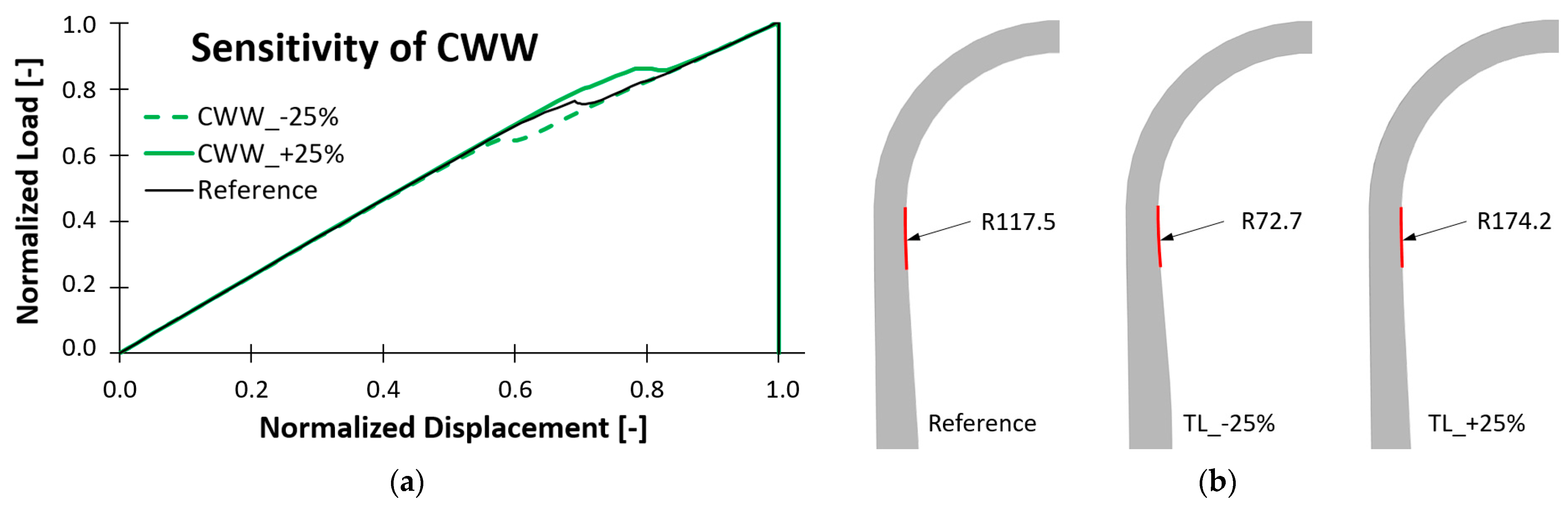
3.2.2. Mechanical Influence of the Characteristic Dimensions

The results of the sensitivity study described in Section 2.2.4 are summarized in Figure 12. Since the macro-model on which the study is based generally predicts a linear elastic deformation followed by abrupt total failure, the mechanical behavior can be summarized well by specifying the calculated spring constant K and the failure load F max . The sensitivity of the varied characteristic dimensions is evaluated based on the resulting K - and F max -deviations compared to the reference model. The variation of LT affects both K (moderately) and F max (more significantly). The deviations of F max are consistent with the stress distribution analyses on tensile-loaded wound loops in [14]: in order to achieve high tensile-load capacity, it is recommended to keep LT small. LT’s influence on K can be explained as follows: the larger the LT, the stronger the wrap area (iii) gets squeezed in the direction of the tensile load (x-direction in Figure 6); since the fibers are transverse to the loading direction at (iii) and E is much smaller than E | | , K decreases with increasing LT. CWI can only be decreased, as it corresponds to the total contact area between the windings and the inserts in the reference model. The decrease of CWI does not cause any significant deviations of K or F max . This is in accordance with the Coulomb friction model described in Equation (1) in which the contact area can be cancelled out of τ lim as well as P [29]. The variation of TL has a significant effect on F max , but not on K . The effect on F max is attributed to the different notch shapes that result from the variation of TL, as shown in Figure 13b. Although the transitions are modeled tangentially in the macro-models, the notch shape still affects the stress distribution in this failure-critical area. It is found that F max decreases, if TL is modeled smaller than measured (−10% and −25%). However, no significant deviation arises when TL is modeled larger than measured (+25%). Finally, the variation of OWS also affects F max , but not K . The reason for the dependence between OWS and F max is that high OWS values induce curvatures within the windings, as can be seen at the top of Figure 6. As the loop is subjected to tensile loading, these curved regions align with the load direction. This is accompanied by a local superposition of tensile and bending loads resulting in stress peaks.
A separate consideration is required for the dimension CWW, which only occurs in meso-models and is therefore investigated using a generic meso-model of the simple loop. Due to delamination, a non-linear deformation is expected even before F max is reached, so that the evaluation of the mechanical influence is based on load-displacement curves in this case. As shown in Figure 13a, the variation of CWW has a direct effect on the onset of delamination, recognizable by the drops in the curves.
The recommendations for geometry modeling derived from the above-described sensitivity study are summarized in Table 5.

3.2.3. Investigation of the Spring Constant K and Adaptation of the Fiber-Parallel Young’s Modulus E | |

To quantify the discrepancy between calculated and measured spring constants observed in [21], both variables are plotted against the winding number in Figure 14a. The black curve represents the mean values of the spring constants measured in the tensile tests on simple loops. The red curve shows the calculated spring constants obtained by computing the respective macro-models while applying the fiber-parallel Young’s modulus ( E | | ) of 26,518 MPa which was originally measured on press-consolidated PP-GF plates in [21]. It can be seen that both variables are linearly related to the winding number, while the curve of the measured spring constants has an inferior slope and is constantly approximately 10% below the curve of the calculated spring constants. These ratios are multiplied by the originally characterized E | | –value of 26,518 MPa to obtain a plot indicating the adapted E | | -values required to recreate the simple loops’ effective elastic behavior. The result is the orange solid curve in Figure 14b. Since the curve is virtually constant, the mean value of 23,953 MPa is henceforth adopted as the adapted fiber-parallel Young’s modulus  E | | of the impregnated PP-GF roving (A), which is assumed to be valid for loop specimens with winding numbers between 2 and 10. The described adaptation of E | | is a temporary solution serving to promptly consider the observed spring constant deviations in the context of FE analyses of fiber skeletons. The authors are aware that it is a simplification which does not replace an in-depth investigation of the underlying physical phenomena. The general applicability of this simplification is tested in Section 3.3 by applying it to the inclined loop.
One potential cause for the above-described spring constant deviation—namely the influence of twisted fibers—is investigated in this work. For this purpose, comparison specimens are made from an artificially twisted commingled yarn, as described in Section 2.1. The twist of 40 turns per meter (Z40) is chosen to be sufficiently high to ensure that it significantly exceeds the process-induced fiber twist which is estimated to be well below five turns per meter and cannot be fully prevented even in the reference samples. The normalized spring constants of both kinds of specimen are given in Figure 15. It is shown that the increased degree of fiber twist generally has a negative effect on the loop‘s stiffness. The spring constants of the specimens with increased fiber twist are 3–10% below those of the reference specimens. Besides the non-ideal fiber orientation, the increased proportion of broken reinforcement fibers is another side effect of the increased fiber twist that certainly contributes to the reduced spring constants. It should be noted, though, that the standard deviations are at a similar order of magnitude as the spring constant deviations. Thus, it is confirmed that fiber twist can be a possible cause of the observed deviations between calculated and measured spring constants. However, the relatively small reduction of the spring constants compared to the high degree of fiber twist suggests that it is not the only and probably not the most significant influence. Another possible cause worthwhile investigating in follow-up work is the potential occurrence of inter-fiber-fractures in the wrap area (iii) during the tensile tests.

3.2.4. Adaptation of the Fiber-Parallel Tensile Strength R | | t

Next to the fiber-parallel Young’s modulus of the impregnated roving (A) described in Section 3.2.3, its fiber-parallel tensile strength R | | t is also adapted in this paper. The reason for this adaptation is the uncertainty associated with the wide range of results obtained when determining R | | t by different methods [21]. Thus, the value found in tensile tests on press-consolidated plates (affected by stress peaks in the clamping area) is 609.0 MPa, whereas the value calculated according to the rule of mixture given in [14] (assuming ideal homogenization) is 1232.2 MPa.
A simple approach to this issue, which is widely used in the design of filament wound structures, is the empirical determination of a reduction factor [9]. This factor serves to reduce the homogenized R | | t -value calculated according to the rule of mixture, so that—based on experimental experience—precise FE simulations of the load-bearing capacity of filament wound structures are enabled.
Following this approach, the macro-models of the simple loops with six and ten windings (simple loops with two windings are not included, as their failure behavior is strongly influenced by delaminations) are simulated using the homogenized R | | t -value of 1232.2 MPa and the resulting failure loads are compared to the ones measured in the tensile tests. The average deviation is taken as the adaptation factor which is then multiplied by 1232.2 MPa. The result of this calculation is 987.9 MPa and is henceforth considered as the adapted fiber-parallel tensile strength  R | | t , which is used in all subsequent simulations. The reduction factor is approx. 0.8 and thus agrees very well with the value given in [9]. Like E | | , R | | t is also validated by application to the inclined loop in Section 3.3.

3.2.5. Comparison of Meso- and Macroscopic Models

A quantitative comparison between the meso- and macro-models of the simple loops is made on the basis of the respectively calculated load-displacement curves. Additionally, two qualitative results—the failure sequence and the failure location—are compared. In order to evaluate the precision of the models, the corresponding measurements and observations from the tensile tests are included in the comparisons.
Figure 16 provides an overview of the deformation and failure behavior of the simple loops with two windings—in the tensile tests as well as in the simulations. Figure 17 summarizes the associated load-displacement curves. As already found in [21], the failure behavior observed in the tensile tests is dominated by delamination. With only two windings, the area of the roving–roving interface is too small to withstand the tensile load until pure fiber fracture is reached. Consequently, the specimens either fail by abrupt/stepwise total delamination or by local delamination followed by premature fiber fracture. In the measured curves (black), both delamination and fiber fracture are manifested by abrupt drops in the measured load. Curves with only one load drop can be classified as abrupt total delamination, while curves with several load drops can either represent a local delamination with subsequent fiber fracture or a stepwise total delamination. The macro-model cannot reproduce delamination processes. It therefore significantly overestimates both the spring constant and the failure load of the simple loop with two windings. It locates the fiber fracture at one end of the wrapping area (iii), as expected in theory [14] and confirmed in several studies [5,8,21], including the present one. This failure-critical point is henceforth referred to as the wrapping flank. The meso-model can reproduce delamination processes and thus, as already shown in [21], achieves a good qualitative agreement with the experimentally observed failure behavior. Quantitative agreement is also good: both the spring constant and the failure load lie within the scatter of the measured curves. The onset of delamination occurs slightly too early. It should be noted that symmetrical modeling of the roving–roving interface results in symmetrical delamination, that is, both ends of the loop delaminate simultaneously. To reproduce the asymmetrical delamination observed in the experiments (either the first or the last deposited winding delaminates first), it is advisable to slightly increase CWW at one end. As shown in Figure 16, this leads to a local delamination of one loop end, followed by premature fiber fracture at the wrapping flank.
The mechanical behavior and the associated load-displacement curves of the (real and modeled) simple loops with six windings are shown in Figure 18 and Figure 19. Although it is hardly recognizable in the figures, local delamination of the loop’s ends also occurs in this case. However, due to the increased area of the roving–roving interface, total delamination is not observed. The local delamination causes a relatively small reduction of the interface area here, manifested by minor drops in the measurement curves. Total failure follows in the form of a fiber fracture at the wrapping flank. This less delamination-dominated behavior is better reproduced by the macro-model. Both the spring constant and the failure load are in the right order of magnitude and the fiber fracture is predicted at the correct location. The ignorance of delamination processes leads to a rather conservative prognosis of the displacement at total failure. The meso-model shows similar results. The only difference is that—as delamination is considered—the displacement lies further within the scatter of the measurement curves. In this case as well, CWW is slightly increased on one end of the loop, to properly reproduce the asymmetric delamination.
The numerical and experimental results obtained for simple loops with ten windings are summarized in Figure 20 and Figure 21. The findings and observations that can be drawn here essentially correspond to the descriptions in the last paragraph (results of the simple loops with six windings). The results of the macro- and meso-models are even more similar in this case, and both agree well with the measurements from the tensile tests.

3.3. Validation of the Presented Approach Using the Example of the Inclined Loop

To validate the presented approach using the example of the inclined loop, the relative tangential displacement between the windings and the inserts (sliding distance) is evaluated as a further reference, next to the sequence and location of failure as well as the load-displacement curves. The results are shown in Figure 22, Figure 23 and Figure 24.
As expected, no recognizable delamination occurs in the tensile tests. Instead, elastic deformation is observed until fiber fracture occurs at one of the wrapping flanks of the small insert. In some cases, not all fibers fail at the same time, which can be seen from the different-sized drops at the end of the measurement curves and is possibly related to an uneven load distribution provoked by the concave insert geometry in combination with the sliding processes occurring at the small insert. The total sliding distance (large and small insert combined) directly before fiber fracture varies between 0.6 and 3.0 mm in the tensile tests, while the sliding processes at the small insert generally account for the larger share of it (74% on average). From video recordings of the tensile tests, it can be seen that stepwise fiber fracture is less likely to occur on specimens with a small sliding distance. Since no delamination occurs, the macro-model is well suited to reproducing the mechanical behavior of the inclined loop. The spring constant as well as the failure load and the maximum displacement lie centrally in the scatter range of the measurements. The location of the fiber fracture is also predicted correctly at one of the wrapping flanks of the small insert. These results indicate that the adaptations E | | and R | | t , as well as the presented geometry modeling approach, generally enable a good reproduction of the inclined loop’s mechanical behavior. To validate the modeling of the insert–roving interface (C), the calculated total sliding distance is considered. At 2.44 mm it is in the upper fourth of the measured range. Since the friction model applied only considers the static friction coefficient (which is higher than the dynamic one), the simulation should, in theory, underestimate the sliding distance. Thus, it can be assumed that the surface of the press-consolidated PP-GF plates used in the friction tests might be smoother than the contact area of the PP-GF windings. Besides, it should be noted that the model locates the greater share (73%) of the total sliding distance at the large insert. This deviation from the measured results is assumed to be related to the idealized geometry modeling approach pursued.

4. Conclusions

In the present work, a systematic approach for FE analysis of thermoplastic impregnated fiber skeletons, initially presented in [21], was advanced and validated. The meso-level geometry modeling procedure was supplemented by further characteristic dimensions whose mechanical influence was subsequently investigated using the example of simple loops. From the results obtained, recommendations for more complex modeling tasks could be derived. With regard to more time-efficient modeling and simulation, the geometry modeling was transferred to the macroscopic level. In a comparison of meso- and macro-modeled simple loops, the application areas of the two approaches were distinguished. Being able to reproduce fiber fracture as well as delamination, meso-models have the potential to provide accurate predictions of deformation and failure for all specimens studied in this paper. Macro-models have the advantage of reduced modeling and computational effort but cannot reproduce delamination and may therefore provide inaccurate results for fiber skeletons that are prone to local or total detachments. These simulation-based findings were confirmed by experimental tensile tests on simple loop specimens. Consequently, it is recommended to rely on macro-modeling only, as long as no major delamination is expected. If this cannot be assured, modeling at the meso-level is required. Based on this finding, the procedures and models developed up to this point were used to generate a macro-model of an inclined loop. In the context of a three-dimensional load transfer and fiber skeleton, a mechanical characterization and modeling of the insert-roving interface (C), as well as some enhancements in the geometry modeling procedure, had to be added. The entirety of the models and procedures developed was validated by experimental tensile tests on inclined loop specimens. Both the qualitative failure sequence observed in the experiments, as well as the measured failure loads and displacements, were reproduced well in the simulations. In order to be able to apply the developed FE analysis approach in the sense of a design engineer, that is, to design and dimension fiber skeletons that are not yet physically existent and cannot be measured, a better understanding and empirical data are required regarding their characteristic dimensions, which are the basis of the proposed geometry modeling procedure.
Consequently, further work will be dedicated to investigating the influence of different process and design parameters on the characteristic dimensions of fiber skeletons. Moreover, the proposed approach will be applied in the context of insert design optimization.

Author Contributions

Conceptualization, J.H.; methodology, J.H. and D.A.; validation, J.H.; investigation, J.H., D.A. and A.K.; writing—original draft preparation, J.H.; writing—review and editing, D.A., B.B., P.E., L.K. and F.H.; visualization, J.H. and D.A.; supervision, F.H.; project administration, J.H. and B.B.; funding acquisition, J.H., B.B. and P.E. All authors have read and agreed to the published version of the manuscript.

Funding

This research was funded by the German Federal Ministry of Education and Research (Bundesministerium für Bildung und Forschung—BMBF), grant number 03VP06670. The APC was funded by the Fraunhofer Publication Fund.

Data Availability Statement

The data presented in this study is available on request from the corresponding author.

Acknowledgments

The authors would like to thank the companies Comfil ApS (Denmark) and Culimeta Textilglas-Technologie GmbH & Co. KG (Germany) for generously providing the artificially twisted PP-GF commingled yarn used in this work.

Conflicts of Interest

The authors declare no conflict of interest. The funders had no role in the design of the study; in the collection, analyses, or interpretation of data; in the writing of the manuscript, or in the decision to publish the results.

References

  1. Minsch, N.; Müller, M.; Gereke, T.; Nocke, A.; Cherif, C. 3D truss structures with coreless 3D filament winding technology. J. Compos. Mater. 2018, 53, 2077–2089. [Google Scholar] [CrossRef]
  2. Büchler, D.; Elsken, T.; Glück, N.; Sier, M.; Bludszuweit, S. Ultraleichte Raumzelle—Entwicklung von ultraleichten Großstrukturen in Faserverbund- und Hybridbauweise für den Schiffbau. In Statustagung Schifffahrt und Meerestechnik—Tagungsband der Statustagung 2011; GmbH, F.J., Ed.; Schriftenreihe Projektträger Jülich: Jülich, Germany, 2011; pp. 25–45. [Google Scholar]
  3. Reichert, S.; Schwinn, T.; La Magna, R.; Waimer, F.; Knippers, J.; Menges, A. Fibrous structures: An integrative approach to design computation, simulation and fabrication for lightweight, glass and carbon fibre composite structures in architecture based on biomimetic design principles. Comput. Des. 2014, 52, 27–39. [Google Scholar] [CrossRef]
  4. Beck, B.; Tawfik, H.; Haas, J.; Park, Y.-B.; Henning, F. Automated 3D Skeleton Winding Process for Continu-ous-Fiber-Reinforcements in Structural Thermoplastic Components. In Advances in Polymer Processing 2020; Hopmann, C., Dahlmann, R., Eds.; Springer Vieweg: Berlin, Germany, 2020; pp. 150–161. [Google Scholar]
  5. Botzkowski, T.; Galkin, S.; Wagner, S.; Sikora, S.P.; Kärger, L. Experimental and numerical analysis of bolt-loaded open-hole laminates reinforced by winded carbon rovings. Compos. Struct. 2016, 141, 194–202. [Google Scholar] [CrossRef]
  6. Holzinger, M.; Loy, C.; Gruber, M.; Kugler, K.; Bühler, V. 3D winding of tailor-made thermoplastic rods for locally reinforced injection molded components. In Proceedings of the 5th International Conference & Exhibition on Thermoplastic Composites ITHEC 2020, Bremen, Germany, 13–15 October 2020. [Google Scholar]
  7. Minsch, N.; Müller, M.; Gereke, T.; Nocke, A.; Cherif, C. Novel fully automated 3D coreless filament winding technology. J. Compos. Mater. 2018, 52, 3001–3013. [Google Scholar] [CrossRef]
  8. Huber, T. Einfluss Lokaler Endlosfaserverstärkungen auf das Eigenschaftsprofil Struktureller Spritzgießbauteile. Ph.D. Thesis, Karlsruher Institut für Technologie (KIT), Karlsruhe, Germany, 2014. [Google Scholar]
  9. Schwarz, M. Gezielte Steifigkeits- und Festigkeitssteigerung von Maschinenbauteilen Durch Vorgespannte Ringarmierungen aus Faser-Kunststoff-Verbunden. Ph.D. Thesis, Technische Universität Darmstadt, Darmstadt, Germany, 2007. [Google Scholar]
  10. Morozov, E.; Lopatin, A.; Nesterov, V. Finite-element modelling and buckling analysis of anisogrid composite lattice cylindrical shells. Compos. Struct. 2011, 93, 308–323. [Google Scholar] [CrossRef]
  11. Woods, B.K.; Hill, I.; Friswell, M. Ultra-efficient wound composite truss structures. Compos. Part A Appl. Sci. Manuf. 2016, 90, 111–124. [Google Scholar] [CrossRef] [Green Version]
  12. Solly, J.; Früh, N.; Saffarian, S.; Aldinger, L.; Margariti, G.; Knippers, J. Structural design of a lattice composite cantilever. Structures 2018, 18, 28–40. [Google Scholar] [CrossRef]
  13. Bellini, C.; Di Cocco, V.; Iacoviello, F.; Sorrentino, L. Performance index of isogrid structures: Robotic filament winding carbon fiber reinforced polymer vs. titanium alloy. Mater. Manuf. Process. 2021, 1–9. [Google Scholar] [CrossRef]
  14. Schürmann, H. Konstruieren mit Faser-Kunststoff-Verbunden, 2nd ed.; Springer: Berlin/Heidelberg, Germany, 2007. [Google Scholar]
  15. Krystek, J.; Kottner, R.; Bek, L.; Las, V. Validation of the adjusted strength criterion LaRC04 for uni-directional composite under combination of tension and pressure. Appl. Comput. Mech. 2010, 4, 171–178. [Google Scholar]
  16. Havar, T. Beitrag zur Gestaltung und Auslegung von 3D-Verstärkten Faserverbundschlaufen. Ph.D. Thesis, Universität Stuttgart, Stuttgart, Germany, 2007. [Google Scholar]
  17. Hashin, Z. Failure Criteria for Unidirectional Fiber Composites. J. Appl. Mech. 1980, 47, 329–334. [Google Scholar] [CrossRef]
  18. Puck, A. Festigkeitsanalyse von Faser-Matrix-Laminaten: Modelle für die Praxis; Hanser: Munich, Germany, 1996. [Google Scholar]
  19. Lapczyk, I.; Hurtado, J.A. Progressive damage modeling in fiber-reinforced materials. Compos. Part A Appl. Sci. Manuf. 2007, 38, 2333–2341. [Google Scholar] [CrossRef]
  20. Kärger, L.; Botzkowski, T.; Galkin, S.; Wagner, S.; Sikora, S.P. Stress analysis and design suggestions for multi-loop carbon roving rosettes to reinforce bolt-loaded open-hole laminates. In Proceedings of the 17th European Conference on Composite Materials ECCM17, Munich, Germany, 26–30 June 2016. [Google Scholar]
  21. Haas, J.; Hassan, O.N.; Beck, B.; Kärger, L.; Henning, F. Systematic approach for finite element analysis of thermoplastic impregnated 3D filament winding structures—General concept and first validation results. Compos. Struct. 2021, 268, 113964. [Google Scholar] [CrossRef]
  22. Camanho, P.P.; Matthews, F.L. A Progressive Damage Model for Mechanically Fastened Joints in Composite Laminates. J. Compos. Mater. 1999, 33, 2248–2280. [Google Scholar] [CrossRef]
  23. Tan, S.C.; Perez, J. Progressive Failure of Laminated Composites with a Hole under Compressive Loading. J. Reinf. Plast. Compos. 1993, 12, 1043–1057. [Google Scholar] [CrossRef]
  24. Tan, S.C. A Progressive Failure Model for Composite Laminates Containing Openings. J. Compos. Mater. 1991, 25, 556–577. [Google Scholar] [CrossRef]
  25. Alfano, G.; Crisfield, M.A. Finite element interface models for the delamination analysis of laminated composites: Mechanical and computational issues. Int. J. Numer. Methods Eng. 2001, 50, 1701–1736. [Google Scholar] [CrossRef]
  26. Ye, J.; Yan, Y.; Li, Y.; Luo, H. Parametric mesoscopic and multi-scale models for predicting the axial tensile response of filament-wound structures. Compos. Struct. 2020, 242, 112141. [Google Scholar] [CrossRef]
  27. Zhang, Y.; Xia, Z.; Ellyin, F. Two-scale analysis of a filament-wound cylindrical structure and application of periodic boundary conditions. Int. J. Solids Struct. 2008, 45, 5322–5336. [Google Scholar] [CrossRef] [Green Version]
  28. DIN EN ISO 8295:2004-10; Plastics—Film and Sheeting—Determination of the Coefficients of Friction (ISO 8295:1995). Beuth: Berlin, Germany, 2004.
  29. ANSYS, Inc. Theory Reference—Release 2020 R2; ANSYS Inc.: Canonsburg, PA, USA, 2020. [Google Scholar]
  30. Rust, W. Nichtlineare Finite-Elemente-Berechnungen mit ANSYS Workbench: Strukturmechanik: Kontakt, Material, große Verformungen; Springer Vieweg: Wiesbaden, Germany, 2020. [Google Scholar]
  31. ANSYS Inc. Structural Analysis Guide—Release 2020 R2; ANSYS Inc.: Canonsburg, PA, USA, 2020. [Google Scholar]
Figure 1. (a) Structural constituents within fiber skeletons, adapted from [21]; (b) Distinction of characteristic areas in a simple loop (shafts (i, ii) and wraps (iii)) and definition of characteristic dimensions, adapted from [21].
Jcs 06 00098 g001
Figure 2. Simple loop specimen with dimensions, adapted from [21].
Jcs 06 00098 g002
Figure 3. (a) Inclined loop specimen after [4] with dimensions; (b) Corresponding winding form.
Jcs 06 00098 g003
Figure 4. Test setups. (a) Simple loop, test setup according to [21]; (b) Inclined loop; (c) Friction test.
Jcs 06 00098 g004
Figure 5. Relation of frictional stress τ and tangential displacement δ in the Coulomb friction model, adapted from [30].
Jcs 06 00098 g005
Figure 7. Meso-models of the simple loops: fiber orientation and characteristic areas (top), close-up view of insert area (bottom).
Jcs 06 00098 g007
Figure 8. Macroscopic geometry model of the inclined loop with characteristic areas (left), screenshot of the 3D measuring (right).
Jcs 06 00098 g008
Figure 9. Detailed illustration of the inclined loop model. (a) Outer wraps; (b) Twisted shafts; (c) Inclination angle.
Jcs 06 00098 g009
Figure 10. Experimental results of the friction tests on PP-GF plate specimens with transverse fiber orientation.
Jcs 06 00098 g010
Figure 11. Convergence studies. (a) Influence of element edge length; (b) Influence of load step size.
Jcs 06 00098 g011
Figure 12. Influence of varied characteristic dimensions on the mechanical behavior of a macro-model.
Jcs 06 00098 g012
Figure 13. (a) Influence of CWW variations on the load-displacement-curve of a meso-model; (b) Notch shapes resulting from TL variations.
Jcs 06 00098 g013
Figure 14. (a) Comparison of measured and calculated spring constants; (b) Corresponding adaptation of E | | .
Jcs 06 00098 g014
Figure 15. Spring constants measured on simple loops with (40 turns/m) and without (<5 turns/m) twisted fibers.
Jcs 06 00098 g015
Figure 16. Deformation and failure behavior of simple loops with two windings (specimens and models).
Jcs 06 00098 g016
Figure 17. Load-displacement curves from tensile tests on simple loops with two windings (measured and calculated).
Jcs 06 00098 g017
Figure 18. Deformation and failure behavior of simple loops with six windings (specimens and models).
Jcs 06 00098 g018
Figure 19. Load-displacement curves from tensile tests on simple loops with six windings (measured and calculated).
Jcs 06 00098 g019
Figure 20. Deformation and failure behavior of simple loops with ten windings (specimens and models).
Jcs 06 00098 g020
Figure 21. Load-displacement curves from tensile tests on simple loops with ten windings (measured and calculated).
Jcs 06 00098 g021
Figure 22. Deformation and failure behavior of inclined loops (specimens and model).
Jcs 06 00098 g022
Figure 23. Load-displacement curves from tensile tests on inclined loops (measured and calculated).
Jcs 06 00098 g023
Figure 24. Sliding processes at the inserts of the inclined loop (specimens and model).
Jcs 06 00098 g024
Table 1. Elastic constants and strength values used in the FE simulations, adapted from [21].
Elastic Constants a
PP-GF roving E | | [MPa] b E [MPa] G | | [MPa] G [MPa] ν | | [-] ν | | [-] ν [-]
23,9533750122511250.320.320.59
Aluminum E [MPa] ν [-]
71,0000.33
Strength Values a
PP-GF roving R | | t [MPa] b R | | c [MPa] R t [MPa] R c [MPa] R | | [MPa] R [MPa]
987.9274.06.744.617.017.8
a ||: parallel to fiber orientation, ⊥: transverse to fiber orientation, t: tension, c: compression; b Values are redetermined in this paper, see Section 3.2.3 and Section 3.2.4.
Table 2. Characteristic dimensions of simple loops with two, six and ten windings.
OWS [mm] a
(Std. Dev.)
TL [mm] b
(Std. Dev.)
AiW [mm2] cLT [mm]
(Std. Dev.)
CWI [mm2] cCWW [mm]
(Std. Dev.)
2 windings(i)0.85 (0.20)15.80 (7.34)2.471.49 (0.24)-0.33 (0.24)
(ii)0.85 (0.20)15.80 (7.34)2.471.14 (0.16)-0.00 (0.00)
(iii)--2.470.90 (0.11)215.561.96 (1.22)
6 windings(i)1.11 (0.22)23.64 (6.39)2.473.34 (0.16)-0.92 (0.32)
(ii)1.11 (0.22)23.64 (6.39)2.472.55 (0.12)-0.49 (0.19)
(iii)--2.471.91 (0.20)304.223.50 (0.41)
10 windings(i)1.18 (0.15)20.78 (6.67)2.472.82 (0.18)-1.60 (0.40)
(ii)1.18 (0.15)20.78 (6.67)2.472.48 (0.11)-1.37 (0.41)
(iii)--2.471.94 (0.08)499.844.64 (0.65)
a Without distinction between the characteristic areas (i) and (ii); b Without distinction between the transitions (i)–(iii) and (ii)–(iii); c Calculated values.
Table 3. Characteristic dimensions and locally present winding numbers of the inclined loop.
OWS [mm] aTL [mm] aAiW [mm2] bLH [mm] c
(Std. Dev.)
CWI [mm2] bCWW [mm]Inclination [°] d (Std. Dev.)N [-]
(i)0.0029.002.475.64 (0.31)-Neglected in macro-model36.58 (0.71)5
(ii)0.0029.002.475.21 (0.06)-36.58 (0.71)4
(iii)--2.4710.84 (1.16)477.3536.58 (0.71)6
(iv)--2.4710.39 (0.31)245.4036.58 (0.71)7
(v)--2.479.20 (0.16)710.78-2
(vi)--2.476.88 (0.29)272.84-2
a Values specified based on the recommendations defined in Section 3.2.2; b Calculated values; c The optical 3D measuring system measures the local loop height, from which the local loop thickness is calculated; d Without distinction between (i)–(iv).
Table 4. Coefficients of friction determined between pressed PP-GF plate specimens and the standard slider made from aluminum.
Friction Coefficients Parallel to Fiber OrientationFriction Coefficients Transverse to Fiber Orientation
μ S | | [-] (Std. Dev.) μ D | | [-] (Std. Dev.) μ S [-] (Std. Dev.) μ D [-] (Std. Dev.)
0.21 (0.03)0.16 (0.02)0.25 (0.05)0.19 (0.02)
Table 5. Recommendations for the determination and modeling of characteristic dimensions.
Char. DimensionMechanical RelevanceRecommendations
LTHighShould be measured in micrographs from each characteristic area and modeled accordingly.
CWILowA measurement is not required. CWI must be greater than zero. It is recommended to use the contact area resulting from the height of the windings.
TLHighShould be measured by means of 2D/3D scans and modeled accordingly.
If this is not possible, it must be ensured that TL is modeled rather too large than too small: 25 % of the distance between the insert centers can be used as a rule of thumb.
OWSHighShould be measured by means of 2D/3D scans and modeled accordingly.
If this is not possible, the shaft should be centered between the wrap endings it connects, knowing that curvatures of the windings and associated stress peaks might be neglected.
CWWHighShould be measured in micrographs from each characteristic area and modeled accordingly.
Publisher’s Note: MDPI stays neutral with regard to jurisdictional claims in published maps and institutional affiliations.

