Influence of Spatially Distributed Out-of-Plane CFRP Fiber Waviness on the Estimation of Knock-Down Factors Based on Stochastic Numerical Analysis

Abstract

The presence of waviness defects in CFRP materials due to fiber undulation affects the structural performance of composite structures. Hence, without a reliable assessment of the resulting material properties, the full weight-saving potential cannot be exploited. Within the paper, a probabilistic numerical approach for improved estimation of material properties based on spatially distributed fiber waviness is presented. It makes use of a homogenization approach to derive viable knock-down factors for the different plies on the laminate level for reference material and is demonstrated for a representative tension loadcase. For the stochastic analysis, a random field is selected which describes the complex inner geometry of the plies in the laminate model and is numerically discretized by the Karhunen–Loeve expansion methods to fit into an FE model for the strength analysis. Conducted analysis studies reveal a substantial influence of randomly distributed waviness defects on the derived knock-down factors. Based on a topological analysis of the waviness fields, the reduction of the material properties was found to be weakly negatively correlated related to simple geometrical properties such as maximum amplitudes of the waviness field, which justifies the need for further subsequent sensitivity studies.

1. Introduction

Composite materials play an important role in many engineering disciplines due to their superior mechanical properties compared to metal. Carbon-fiber-reinforced polymers (CFRP) are a key ingredient for the construction of efficient aircraft vehicles in order to reduce structural weight and fuel consumption.

Yet, the use of composite materials induces several challenges along the entire development chain due to higher complexity in component manufacturing in contrast to metallic counterparts. Due to that, process-induced defects may arise which mainly depend on the type of underlying manufacturing technology, e.g., automated fiber placement [1]. The presence of such inhomogeneities within the material leads to a degradation of the load-bearing capabilities of the structure and favors crack initiation, which needs to be handled. Due to a lack of experience, companies are, therefore, often forced to rely on conservative designs with minimum defects to comply with quality and safety requirements. This leads to high manufacturing effort and cost. Therefore, knowledge about the influence of material flaws on the structural integrity of lightweight components based on CFRP materials is essential for developing structural designs in favor of an overall cost reduction and increased life cycle of the components.

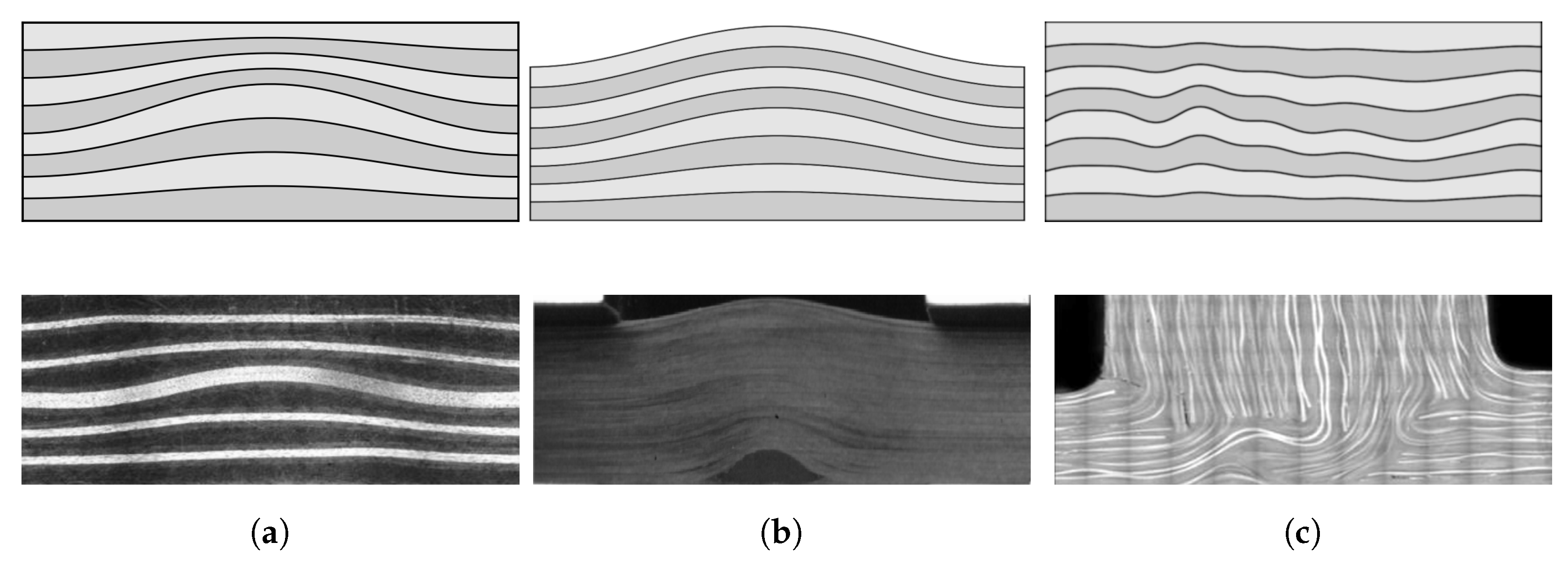
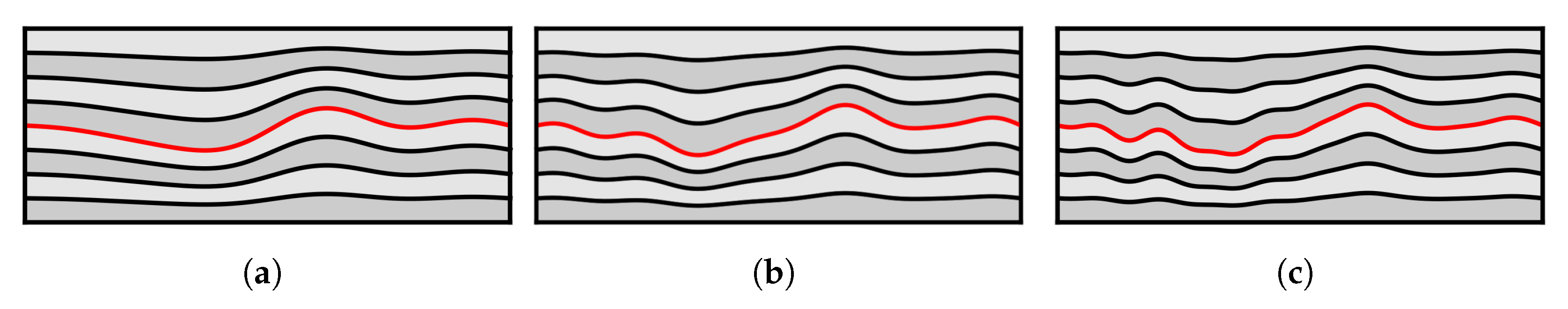
1.1. Out-of-Plane Waviness

One relevant defect is fiber undulation, which may result in either an in-plane angle misalignment of a composite layer or an out-of-plane waviness formation through the entire thickness of the laminate. This type of defect may be induced, e.g., in resin transfer molding or autoclave processes based on pre-preg materials [2,3]. The latter is defined as a reference process for further considerations within this contribution. Due to the manifold origins of wavy formations in the material, it is difficult to comprehensively describe the undulation pattern within complex structural parts. However, a systematic overview is given in [4] on different aspects of out-of-plane fiber waviness, e.g., geometric classification schemes. Without a claim of completeness, Figure 1 shows some exemplary conceptual waviness classifications.

The phenomenological analysis of waviness in fiber composites with respect to the correct assessment of resulting material properties is, even for simple test cases and load settings, a part of ongoing research. One of the first attempts to describe the effect of fiber waviness on mechanical behavior can be found in [8]. The main focus of the first research investigations laid on analytical or semi-analytical models to describe the complex interaction between fiber and matrix within the material to accurately predict crack initiation under different load cases and the determination of stiffnesses and residual strengths [9,10]. The approaches developed differ with respect to the depth of detail considered and the mechanical behavior that can be represented. Due to the complex mechanical behavior, the existing calculation methods were often limited to two-dimensional problems and simple geometries. With the advent and versatile applications of finite element methods (FEM), more complex waviness geometries have been investigated [11,12]. Meanwhile, other methodological approaches using mesh-free numerical methods were developed to estimate material degradation and failure propagation in damaged composite materials more precisely [13]. However, they still lack in terms of a fast assessment of reduced material properties in a stochastic view due to its higher computational complexity.

Despite the ability of new numerical methods to capture a complex material behavior in terms of strength and stiffness, its extensive use in practical applications still relies on experimental validation approaches [14,15,16,17]. One main challenge of this is to assure high repeating accuracy of the specimen tests with artificial defects due to many sources of errors in the testing structure. Within the physical testing procedures, optical measurement techniques such as digital image correlation [18] are frequently used for the correct detection of crack initiation and propagation in composite materials. As a consequence, they are often limited to a cross-sectional image analysis, which excludes waviness defect analysis of higher three-dimensional complexity. Other approaches such as computer tomography scans may be an alternative but often involve higher costs of the measuring tools and further issues in image-based reconstruction.

1.2. Spatial Stochastic Analysis

As already mentioned in the beginning, the presence of material defects such as out-of-plane waviness is treated with conservative rules in manufacturing and design to fulfill high quality requirements. These rules aim to include effects of discrete waviness defects which are often provoked due to the selected manufacturing technology and an unforeseen, additional random waviness pattern whose detection is hard to predict in general. For the latter, deterministic numerical approaches in the literature are not sufficient, as previously shown. Therefore, stochastic analysis methods which combine the physical representation of local inhomogeneities with a random spatial distribution are essential.

With the help of increasing computation resources, the treatment of spatially distributed uncertainties in mechanical engineering with respect to composite applications is considered more frequently in the last decade [19]. Due to numerous possible CFRP material configurations based on complex stacking sequences in general, stochastic analysis of spatial material uncertainties available in the literature usually focuses on partial aspects of different material length scales, ranging from the microscopic level to the component level, partially with the attempt to combine the different levels through a multiscale approach [20]. At the microscopic level, Arai et al. [21] demonstrate a probabilistic approach for the spatial modeling of the microstructure of composite material containing fibers and matrix components based on scanning electron microscope images. The authors of [22] propose a similar approach for the determination of the Young’s modulus of short-fiber reinforced composites extended by an experimental verification based on tensile tests. In [23], a methodology is presented to spatially model local deviations of the fiber volume fraction with a focus on frequency analysis of a representative composite panel. Based on experimental studies, it was shown that in the case of particular natural frequencies a numerical modeling approach incorporating spatial material properties may result in a better alignment with results from physical tests compared to an averaged modeling approach. Zein et al. [24] propose a method to simulate spatial distributions of the fiber volume fraction over a largely curved composite structure with a focus on stiffness and strength analysis and different geometrical parameters. In [25], a quantitative assessment of the buckling stability of composite cylinders is presented under consideration of spatially varying imperfection within the structure based on optical measurements. Additionally, in [26], the benefits of efficient stochastic simulation methods are shown based on a multilevel Monte Carlo approach. The developed method was demonstrated on a two-dimensional composite plate subjected to a spatial fiber angle deviation. Sutcliffe et al. [27] investigated the size effect of random fiber angles relative to specimen dimensions in terms of compressive strength. Besides the versatile applications and studies in the literature, extensive data from physical measurements in terms of spatial distribution are still missing and remain a challenge in the reliable numerical analysis including spatial aspects [28]. In [19], a numerical evaluation of stochastic distributed out-of-plane fiber wrinkles in a CFRP material was done with a focus on corner bend strength issues applied to a wing spar structure as an industrially motivated case study. Based on computer tomography scan data, the complexity of the fiber wrinkle parametrization was reduced to one model parameter through the thickness of the laminate with a constant extension of the defect along the depth direction of the representative spar structure. Despite the numerical abilities of the proposed approach, challenges still remain due to the worse validity of the estimated defect distributions and causal relationships between the mechanical response and defect geometry dimensions for generic use on any kind of composite structure.

Based on the literature and to the best knowledge of the author, there is still a lack of profound studies concerning the three-dimensional spatial stochastic modeling and assessment of composite fiber waviness on the laminate level with respect to the material strength issues. This contribution thus tries to fill this gap by proposing a pragmatic numerical approach for the estimation of strength properties within that physical problem space. As a further beneficial target, the proposed approach shall give possibilities to derive influence parameters of complex waviness distributions, which could be used for a competitive composite component analysis in industrial-like scenarios.

The paper starts by explaining the underlying theory to compute specific material properties. Subsequently, the implemented spatial stochastic modeling and numerical assessment method will be described. Selected results with respect to specific model and material parameters will be shown and discussed in detail. Finally, a conclusion will be drawn from the achieved results, and an outlook will be given.

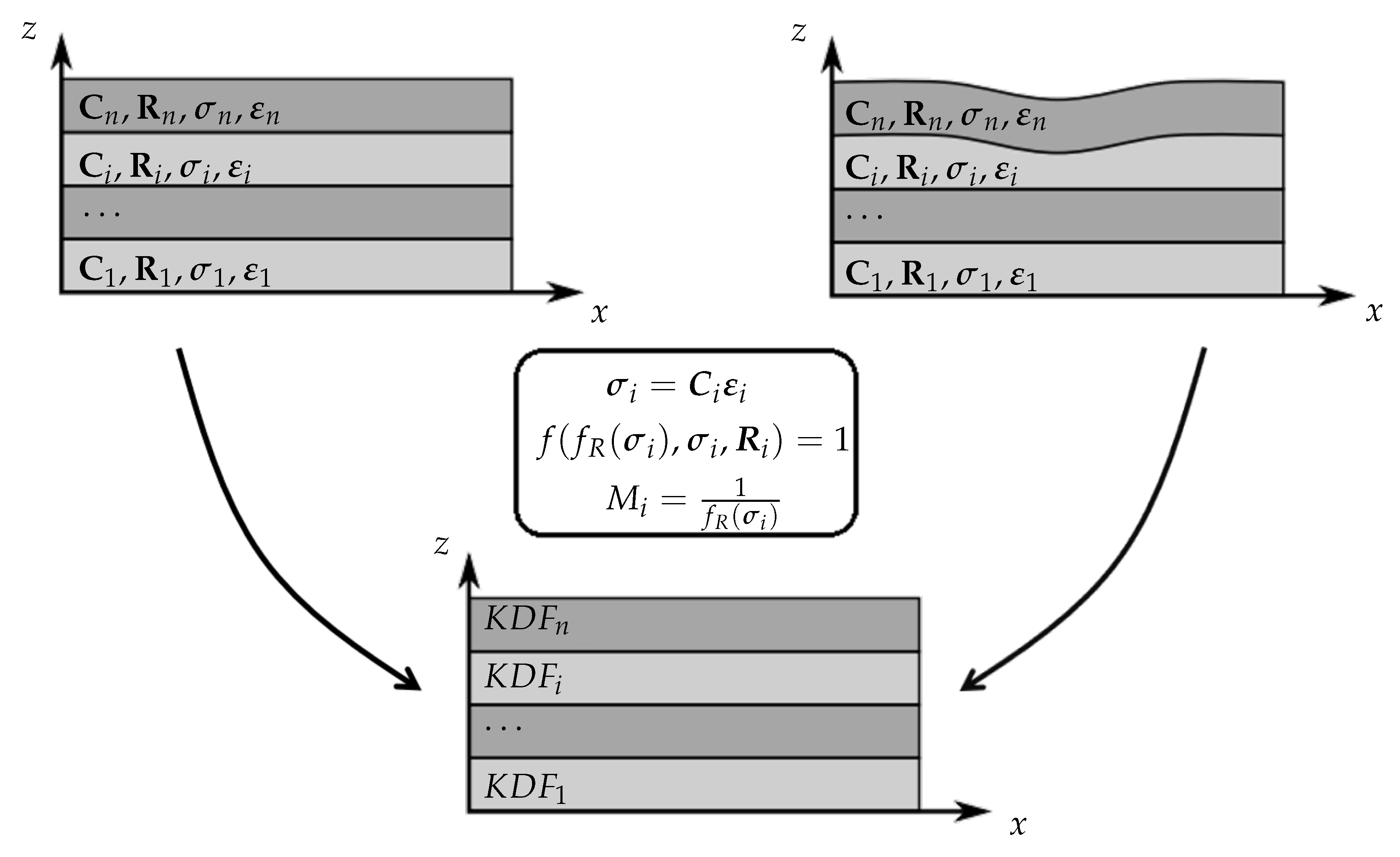
2. Multiscale Analysis for Computation of Knock-Down-Factors

Prior to the stochastic considerations, an appropriate methodology to assess the mechanical effects of fiber waviness needs to be defined. The modeling approach described in detail in the following is based on the observation that imperfections in a multilayer laminate often affect not only one layer but also neighboring layers through phenomena such as load redistribution and mechanical stress localization. The proposed method is suitable for both the determination of the effective elastic and strength properties of a material (see also [12,29]). The approach considers the entire laminate for the homogenization of defects and not only the individual ply. On the mesoscale (laminate level), these detailed models provide the homogenized structural response from boundary conditions applied on the macroscale (structural level). The determined so-called knock-down factors (KDF) map the influence of defects on the material properties. The selected modeling approach thus enables the analysis of local imperfections at the ply level, detached from the global structure analysis. Imperfections occurring in a local area of the laminate or global structure can be analyzed separately using this approach. The validity of the structural response determined in this way is limited to the considered region. This loss of representativeness in the narrower sense is compensated by the fact that an unlimited number of analyses can be performed in advance with the corresponding configuration of the local three-dimensional model. Within the scope of the publication, only tensile strength considerations based on a generic laminate are carried out to demonstrate the multiscale approach. For the corresponding analysis, the stress-based Puck failure criterion [30] is used for the computation of the internal material limit state of the analysis model.

A stress-based failure criterion is a function f of the current mechanical stress state $\mathbf{\sigma }$, and the strength properties $\mathbf{R}$ of the material. It converts $\mathbf{\sigma }$ into a scalar value, often referred to as the failure index (FI):

$$\begin{array}{c}\hfill f\left(\mathbf{\sigma },\mathbf{R}\right)=\mathrm{FI}.\end{array}$$

(1)

The equation $f(\mathbf{\sigma },\mathbf{R})=1$ specifies a limit state, which describes the mechanical stress limit of the material in the six-dimensional stress space. The mechanical stress space is six-dimensional when using the index-based vector-matrix form (Voigt notation). As soon as $f(\mathbf{\sigma },\mathbf{R})$ exceeds $1$, material failure has occurred. The intersection points of the stress axes with the limit surface correspond to the strengths under uniaxial loading.

For each vector in the stress space, there is a positive factor $f_R\left(\mathbf{\sigma }\right)$, usually called reserve factor, which maps this stress state to the interface of the failure body [30]:

$$\begin{array}{c}\hfill f\left(f_R\left(\mathbf{\sigma }\right),\mathbf{\sigma },\mathbf{R}\right)=1.\end{array}$$

(2)

Computationally more advantageous, though, is the use of the so-called material effort M, since the reserve factor $f_R\left(\mathbf{\sigma }\right)$ becomes infinite for $\parallel \mathbf{\sigma }\parallel =0$. The material effort M converts a vector from the six-dimensional stress space into a scalar. This scalar represents the utilization coefficient with respect to the strength limits of the material. In a general form, the material stress M results from evaluating any failure criterion $f(\mathbf{\sigma },\mathbf{R})$. For failure criteria $f(\mathbf{\sigma },\mathbf{R})$ that are homogeneous from degree k in $\mathbf{\sigma }$, M is calculated as follows:

$$\begin{array}{c}\hfill M=\frac{1}{f_R\left(\mathbf{\sigma }\right)}.\end{array}$$

(3)

The determination of M is more demanding if the formulation of the failure criterion contains different polynomial degrees of $\mathbf{\sigma }$. The material effort M determines the load that can still be tolerated by the material until failure [31,32]. Multiplying the stress vector by the reciprocal of M (a uniform increase of all stress components) results in the failure load [30]. For example, if the material stress is $M=0.5$, 50% of the material load limit is reached.

The determination of the effective strength properties is done utilizing finite element (FE) analyses. The solution of nine uniaxial load cases results in stress distributions from which the effective strength values for the laminate and the individual layers are determined. Each load case is evaluated using selected stress-based failure criteria with regard to damage initiation in the individual layers. This involves comparing each laminate with imperfections with the corresponding pristine reference laminate. Both models (imperfect and nominal) are created and analyzed with identical FE meshes, boundary conditions, and loads. Figure 2 outlines the layer-by-layer evaluation of the resulting stress distributions in the imperfect and reference laminate. According to Equation (3), the finite element with the highest material effort ($M_i^{\mathrm{def}}$) is identified in each single layer i of the laminate with imperfection. Using the same failure criterion, the material effort ($M_i^{\mathrm{ref}}$) of the matching finite element of the reference laminate is determined in parallel in the same layer i of the FE mesh. For failure criteria that distinguish between different failure modes (the selected Puck criterion in this contribution), the material effort is calculated based on the failure mode, which is likely to initiate material damage first compared to other modes.

The ratio of these layer-by-layer material efforts ($M_i^{\mathrm{ref}}$ and $M_i^{\mathrm{def}}$) equals the reduction factor (KDF) of the assigned strength parameter for each uniaxial load case [33,34]:

$$\begin{array}{c}\hfill {\mathrm{KDF}}_i=\frac{M_i^{\mathrm{ref}}}{M_i^{\mathrm{def}}}=\frac{f_R^{\mathrm{ref}}\left({\sigma }_i\right)}{f_R^{\mathrm{def}}\left({\sigma }_i\right)}.\end{array}$$

(4)

From Equation (4), nine ratios can be obtained for $R_x^{(+)\mathrm{def}}$,$R_x^{(-)\mathrm{def}}$, $R_y^{(-)\mathrm{def}}$, $R_x^{(-)\mathrm{def}}$, $R_z^{(+)\mathrm{def}}$, $R_z^{(-)\mathrm{def}}$, $R_{\mathrm{xy}}^{\mathrm{def}}$, $R_{\mathrm{xz}}^{\mathrm{def}}$, and $R_{\mathrm{yz}}^{\mathrm{def}}$ for each individual layer. The superscripts indicate whether it is a property of the imperfect ${(\ast )}^{\mathrm{def}}$ or the nominal laminate ${(\ast )}^{\mathrm{ref}}$. For demonstration purpose of the approach, the KDF for tensile strength $R_x^{(+)\mathrm{def}}$ will be used exemplarily as part of selected analysis studies described in Section 4 and Section 5.

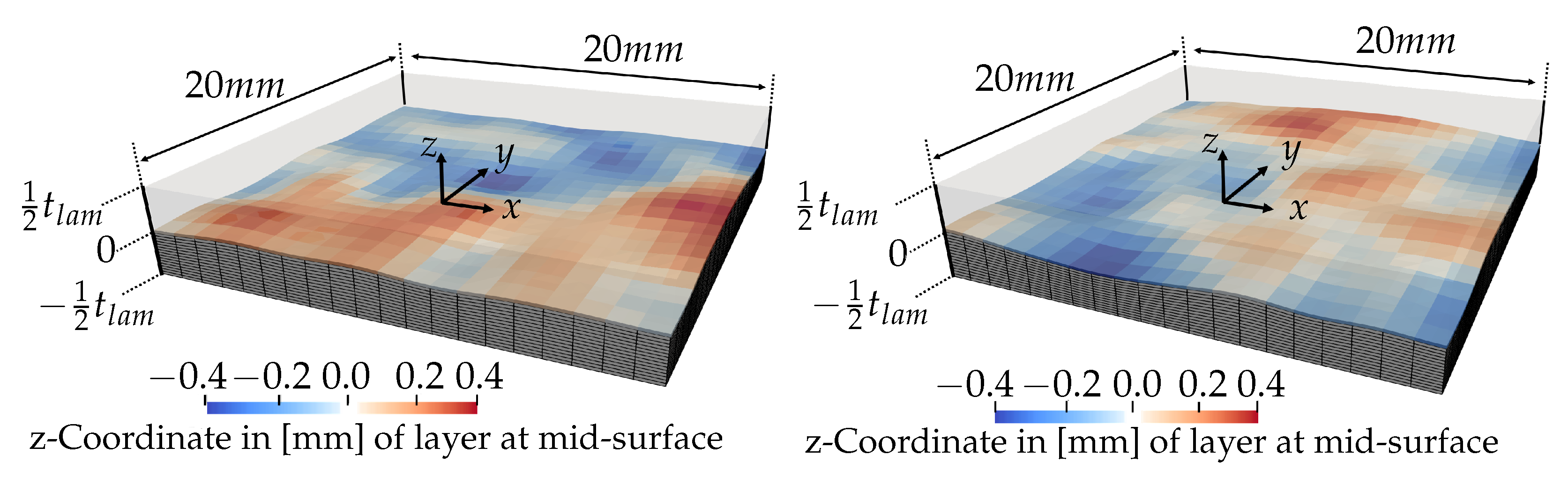
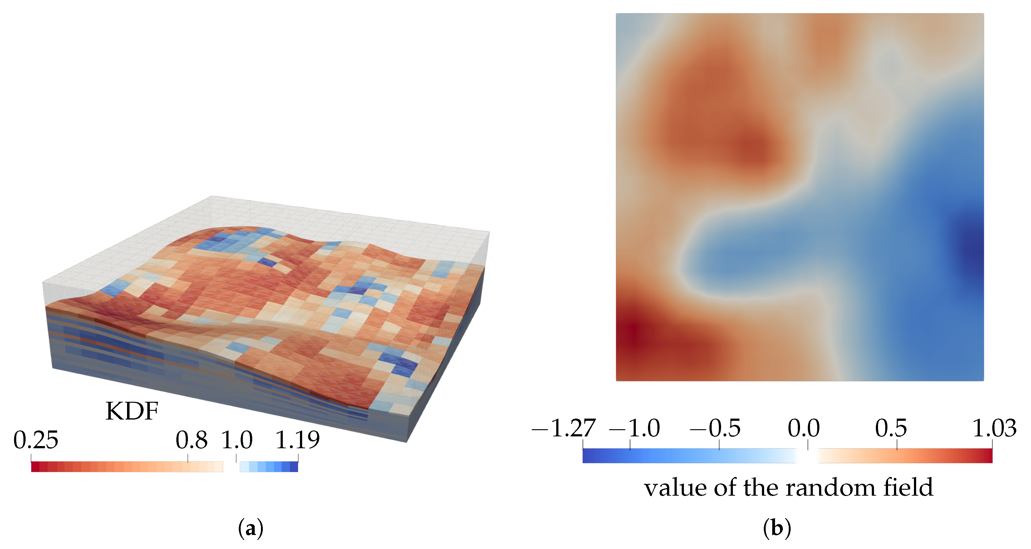
3. Random Field Analysis

For the derivation of an appropriate approach to model the variety of typical out-of-plane fiber wrinkle geometries, the so-called random field concept [35] is used within this contribution. Used for decades in other scientific disciplines already, the approach is also frequently applied in recent stochastic mechanical analysis studies of CFRP materials, as already presented in Section 1.2.

From a mathematical point of view, a random field $H(\mathbf{x},\theta )$ can be considered as a random function that characterizes a random quantity at each point $\mathbf{x}\in \Omega$ of a continuous domain $\Omega \subset {\mathbb{R}}^d,d\in {\mathbf{N}}_{>0}$. The quantity $\theta \in \Theta$ represents a coordinate in the sample space $\Theta$. Besides its multidimensional definition, the parameter d usually represents the considered physical space dimension in real-world problems, namely one, two, or three dimensional. For modeling aspects within the paper, the random field $H(\mathbf{x},\theta )$ represents the out-of-plane deformation $\theta$ due to the wrinkling of a material point in the CFRP material at a specific spatial position $\mathbf{x}\in {\mathbb{R}}^2$. In case of a one-dimensional problem, an example of an undulation within a laminate with help of the random field is shown in Figure 1c. Furthermore, the deformation of a material point is assumed to vary symmetrically to a mean value relying on a normal distribution so that so-called Gaussian random field methods can be used for simulation. One main fundamental characteristic property of a Gaussian field is the fact that it can be described by its second-order statistics, the mean function $\mu :\Omega \to \mathbf{R}$, and covariance function $Cov:\Omega \times \Omega \to \mathbf{R}$. For ease of use, the assumption of centered Gaussian fields with zero mean is made for this contribution.

3.1. Covariance Function

In general, the covariance function is an extension of the covariance matrix defining the dependency between two or more random variables. The major difference is the definition of a term describing the spatial relation between two random variables at points $\mathbf{x}$ and ${\mathbf{x}}^{\prime }$ within the random field $H(\mathbf{x},\theta )$. Formally speaking, this can be described by the equation

$$Cov(\mathbf{x},{\mathbf{x}}^{\prime })=s^2·\rho (\mathbf{x},{\mathbf{x}}^{\prime })$$

(5)

where s represents the variance of the quantity $\theta$ and $\rho (\mathbf{x},{\mathbf{x}}^{\prime })$ describes the correlation model between two points of the random field. While not restricted to a special kind of correlation function, covariance matrices for a given subset of points in the random field always need to be positive-definite. An example of a spatial correlation model used in different disciplines in science and engineering is the so-called Matern-kernel function

$$\rho (\mathbf{x},{\mathbf{x}}^{\prime })=\frac{1}{\Gamma \left(\nu \right)2^{\nu -1}}\frac{\sqrt{2\nu }}{l}d{(\mathbf{x},{\mathbf{x}}^{\prime })}^{\nu }{K}_{\nu }\left(\frac{\sqrt{2\nu }}{l}d(\mathbf{x},{\mathbf{x}}^{\prime })\right)$$

(6)

where $\nu$ and l are positive parameters, $\Gamma$ represents the Gamma function, and $K_{\nu }$ the modified Bessel function. The function $d(\mathbf{x},{\mathbf{x}}^{\prime })$ describes a distance function between two points within a random field based on a metric, e.g., the Euclidean distance. Based on Equation (6), a large variety of different kernel models can be implemented, which can be seen in Figure 3. In the case that $\nu$ equals to 0.5, Equation (6) simplifies to a simple exponential kernel function with

$$Cov(\mathbf{x},{\mathbf{x}}^{\prime })=s^2·e^{-{∥\frac{\mathbf{x}-{\mathbf{x}}^{\prime }}{\mathbf{l}}∥}_2}$$

(7)

which is a specific realization of the Matern kernel and already used in composite waviness analysis [19,36].

3.2. Numerical Discretization

Due to the complex nature of physical problems with many degrees of freedom, the use of the random field as previously described is neither appropriate nor technically viable. To overcome this, the key to an efficient analysis with inherent spatial variability is a numerical discretization scheme that approximates the original random field with a few random variables. A lot of discretization methods have been published in the literature. Among other series expansion methods, the Karhunen–Loève expansion (KLE) is frequently used due to its optimality in terms of global error metrics [37]. It is based on the spectral decomposition of the autocovariance function (often also referred to as the kernel function) of the random field [38]. In general, it states that an ordinary second-order random field can be represented exactly as follows:

$$H(\mathbf{x},\theta )=\mu \left(\mathbf{x}\right)+\sum _{i=1}^{\infty }\sqrt{{\lambda }_i}{\phi }_i\left(\mathbf{x}\right){\xi }_i\left(\theta \right)$$

(8)

In Equation (8), $\mu \left(\mathbf{x}\right)$ represents the mean function of the field, and ${\xi }_i\left(\theta \right)$ describes standard uncorrelated random variables. The parameters ${\lambda }_i$ and ${\phi }_i\left(\mathbf{x}\right)$ represent the eigenvalues and eigenfunctions of the autocovariance kernel. They can be obtained by solving the homogeneous Fredholm integral equation of the second kind:

$${\int }_{\Omega }Cov(\mathbf{x},{\mathbf{x}}^{\prime }){\phi }_i\left({\mathbf{x}}^{\prime }\right)d{\mathbf{x}}^{\prime }={\lambda }_i{\phi }_i\left(\mathbf{x}\right)$$

(9)

Within this paper, it is assumed the random field describing the fiber waviness has a zero mean, so the corresponding term $\mu \left(\mathbf{x}\right)$ has no contribution to the random field. The analytical solution of the integral eigenvalue problem given in Equation (9) is only applicable for a few autocovariance functions and simple geometric shapes as the definition of the global domain. Therefore, the eigenvalue problem is solved numerically. This leads to a truncated, numerical approximation of the KL expansion given in Equation (8) as follows:

$$\hat{H}(\mathbf{x},\theta )=\mu \left(\mathbf{x}\right)+\sum _{i=1}^N\sqrt{\widehat{{\lambda }_i}}\widehat{{\phi }_i}\left(\mathbf{x}\right)\widehat{{\xi }_i}\left(\theta \right)$$

(10)

In Equation (10), $\widehat{{\lambda }_i}$ and $\widehat{{\phi }_i}$ are now approximations to the eigenvalues ${\lambda }_i$ and eigenfunctions ${\phi }_i$ of length N, respectively. N directly affects the accuracy of the random field variations to be modeled, but also increase the computational effort of the solution of the eigenvalue problem. Depending on the physical problem to be solved and given input data, the number of N eigenvalues is usually in the order of 50–150. A one-dimensional example of a single random field realization related to the fiber waviness modeling problem with a different number of eigenvalues is demonstrated in Figure 4. For the estimation of the eigenfunctions, different numerical algorithms exist in the literature [38].

4. Probabilistic Analysis

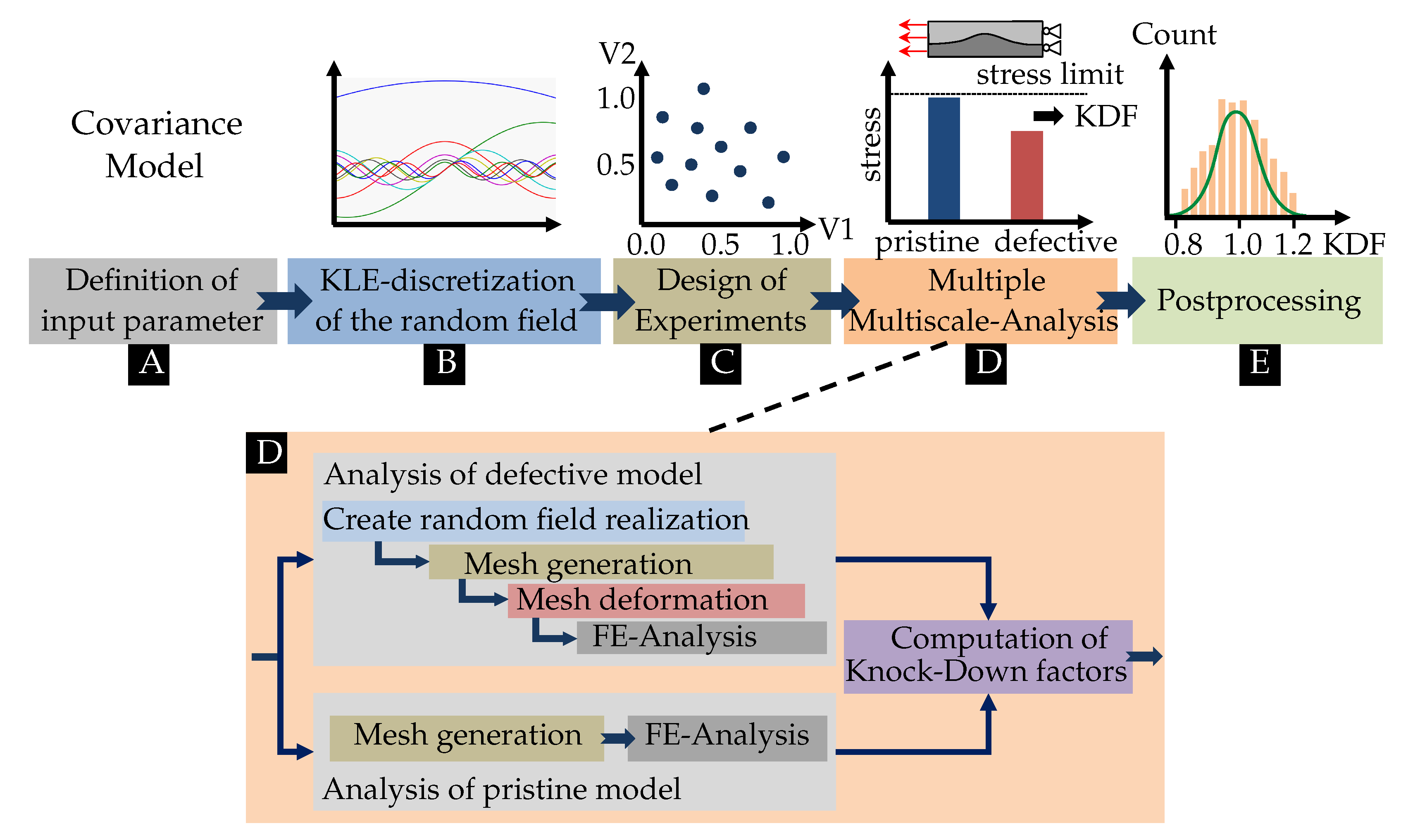
4.1. Process Description

Numerical analyses of mechanical problems under the influence of randomly distributed disturbances can be divided into two categories from the methodological point of view: intrusive or non-intrusive methods. The former describe the direct coupling of stochastic random field formulation and mechanical problem formulation to determine resulting stochastic output quantities [39]. In the following, the latter, non-intrusive method will be used, which offers advantages from an implementation point of view by separating the stochastic and the mechanical problem and is frequently used in the literature [40]. Figure 5 shows a corresponding graphic representation of the process implementation as a base for stochastic analysis of this contribution. As a consequence of the chosen KLE-based approximation of the waviness random field (Box A and B) and as a prior step of the numerical KDF computation in Box D, a statistical design of experiments is carried out which generates the different types of random waviness realization from the base field. Due to the non-intrusive nature, independent analysis between the different waviness field samples can be conducted. Each of these distinct waviness fields represent the model input for the deterministic determination of the knock-down factors (Block D). As already mentioned in Section 2, the numerical computation of the mechanical response under the influence of fiber waviness is obtained by using black box FE models. Based on the deterministic KDF results for each sampled waviness field, histograms and distribution functions can be easily determined for each selected material parameter in the individual layers of the laminate (Block E).

4.2. FEM Modeling

Related to the deterministic computation (Block D) in the stochastic analysis process, three-dimensional FE models are generated with discretized parts representing the individual layers of the laminate through distinct solid elements assigned with unidirectional material properties. The different plies are connected through coincident nodes neglecting cohesive zone effects. An example using a three-dimensional FE model approach for two selected random field samples is shown in Figure 6. In order to represent the existing mechanical stress distribution across the layer thickness physically appropriately, a quadratic deformation approach using 20-node solid elements is chosen in the FE model [41] due to its favored numerical convergence properties and less sensitivity against shear locking compared to linear elements.

The initial modeling step is a structured mesh generation of the laminate configuration using the open-source tool Gmsh [42]. Subsequently, a mesh deformation of each layer in the material is performed according to the previously generated random field samples at the laminate midsurface to generate the desired three-dimensional model defects. An essential advantage in comparison to unstructured mesh methods, which could locally better resolve the random field, is the usability within stochastic analysis. For the FE-based determination of the material properties and stresses of the undisturbed laminate, a structured mesh has to be generated only once initially, so that significant time and resource savings can be achieved due to the computational scope at hand. For reasons of complexity, a laminate configuration is chosen in the publication in which the waviness is pronounced in the interior of the material and tapers off to the two outer layers. In this case, the middle layer in the laminate experiences the maximum deformation due to waviness.

Finally, using the deformed inner laminate geometry, a linear-static calculation is performed for the pristine laminate without waviness and defective configuration applied to each selected material property. According to Section 2, for each property, there exists a uniaxial loadcase and boundary condition which is to be applied consequently to the model prior to the numerical calculation of the mechanical response. For tensile strength analysis in the x-direction as an example in this paper, the corresponding unit loads and boundary conditions are shown in Figure 7 and

Table 1. Applied values for boundary conditions to node sets and loads of the model.

x-Direction	y-Direction
$u^{yzP{I}^{-}}=0$	$u^{xzP{I}^{-}}=0$
$u^{yzP{I}^{+}}=u^{N^{ref}}$	$u^{xzP{I}^{+}}=0$
$F_x=\sigma ·A^{yzP{I}^{+}}$ $\sigma =1$

. They enforce a macroscopic uniaxial strain state within the model.

Due to the probabilistic and computational needs, the study makes use of the open-source FE program B2000++ [43] to compute the model deformation and internal mechanical stresses.

5. Results

5.1. Parameters

In the following section, the results of probabilistic analysis studies will be presented, considering selected parameters and characteristics, which were obtained using the previously described calculation approach. Within the study, the CFRP material IM7/8551-7 was selected as reference a for the material properties of the unidirectional layers used within the numerical model [44]. For the sake of simplicity, the material properties are assumed to be constant over the physical domain in each of the plies. Local deviations, which may occur due to regions with an excess of resin and a high-volume fraction of fibers induced by the complex waviness distribution and a corresponding non-uniform thickness distribution, are neglected. This assumption is valid for small to moderate waviness amplitudes but should be questioned critically in the case of larger waviness amplitudes. As a stacking sequence, a symmetric laminate with 32 plies as typically used in aerospace is chosen:

$${[45,0,-45,90,45,0,0,45,0,-45,0,0,45,90,45,0]}_S$$

This configuration is selected from a representative result of a structural optimization on the structural component level [45,46]. Based on a single-ply thickness of $0.125$ $\mathrm{m}$$\mathrm{m}$, the total thickness of the laminate reference configuration is 4 $\mathrm{m}$$\mathrm{m}$. The length and width of the reference were initially set to 20 $\mathrm{m}$$\mathrm{m}$ symmetrically. For the description of the random field, a two-dimensional exponential model is used

$$Cov(\mathbf{x},{\mathbf{x}}^{\prime })=s^2·e^{-{∥\frac{\mathbf{x}-{\mathbf{x}}^{\prime }}{\omega }∥}_2}$$

(11)

with the following parameters to calculate the covariance matrix.

$$\omega =\left(\begin{array}{c}{\omega }_1\\ {\omega }_2\end{array}\right)=\left(\begin{array}{c}5\\ 5\end{array}\right)\mathrm{mm} and s^2=0.25$$

(12)

The nominal values for the correlation length and stochastic variance of the waviness amplitude chosen for the numerical studies rely on data from the literature [28]. They are adopted subsequently in this context according to the initially selected autoclave process as a manufacturing use case. This is done by the fact that available data were acquired for materials with a layup orientation of predominantly zero degrees. Since the selected laminate configuration used in the following numerical studies differs significantly, the chosen spatial stochastic parameters were initially assumed to be more conservative with a potential slightly higher amplitude. However, this step needs to be validated by an extensive experimental campaign which is a remaining issue of this contribution to be addressed in the future. Combined with the geometrical dimension of the reference model, a ratio between the correlation length of the random field and the geometrical model size results in 0.25 for the selected numerical study. For a comprehensive analysis of the stochastic problem description, it is to be addressed whether the ratio has an influence on the distribution of the resulting KDF. Since this involves further computationally demanding studies this issue is not taken into consideration in this contribution.

Based on the selected random field model, the numerical approximation of the covariance matrix using the KL approach is done with the software library OpenTURNS [47]. For the design of experiments as part of the stochastic evaluation process shown in Figure 5, an ordinary Latin hypercube sampling method [48] is used to sample the uncorrelated normal variables for the particular eigenfunctions. The method is modified to slightly favor the first eigenfunctions compared to higher modes.

Due to the high computational requirement, all conducted studies were executed on a high-performance computer. For computing purposes, the so-called HPC cluster CARA was used, located at the German Aerospace Center in Dresden, Germany. It comprises nearly 146,000 physical CPU cores in total, distributed on 2280 compute nodes based on AMD EPYC 7601 processors. Each node provides 128 GB of physical memory. Due to the high I/O throughput of the different steps in the implementation of the numerical approach, only 500 cores assigned with a single stochastic sample computation each were used within each of the studies.

5.2. Deterministic FE Analysis

As a precedent step of the stochastic analysis, a deterministic analysis of a specific realization of the random field was made to verify the numerical approach, as explained in Section 2 and Section 3. In Figure 8a, the results of the KDF computation using the model parameters of Section 5.1 are shown and highlighted for the ply at half of the laminate thickness. In addition, Figure 8b shows the corresponding realization of the random field with parameters described in the previous section.

In

Table 2. Computation time.

	Computation Step	Elapsed Time
	FE model generation	31.75 s
Defective	FE analysis	120.09 s
	Result postprocessing	5.44 s
	FE model generation	25.75 s
Pristine	FE analysis	112.83 s
	Result postprocessing	5.30 s
	KDF estimation	10.53 s
	Total runtime	311.69 s

, the required computation time for different process steps of the KDF computation based on a deterministic analysis of the defective and pristine configuration is illustrated. As expected, most of the runtime is taken by finite element computation.

In order to evaluate the mechanical problem in a statistically appropriate manner, an initial convergence study was conducted to find out suitable parameters in terms of the mesh densities of the underlying finite element model used. Initially, the mesh density in the x-direction coincident with the load direction of the selected loadcase was varied for each of the layers of the laminate, leading to numerical model size between 50 and 350 thousand degrees of freedom. Compared to the geometric dimension of the model, the element edge length in the x-direction lies between $0.4$ $\mathrm{m}$$\mathrm{m}$ for the finest mesh size and $1.0$ $\mathrm{m}$$\mathrm{m}$ for the coarsest mesh configuration. Figure 9 shows the results of the computed KDF for the upper half of the ply of the selected laminate configuration. Due to the homogenization approach and the waviness parametrization on the midsurface of the symmetric laminate, the KDF of the lower laminate plies can be assumed to be nearly equal to the values of the upper laminate layers and, therefore, can be skipped here for better readability.

In Figure 9 it can be seen that, except for a few plies, the resulting KDF of the different layers of the laminate lie in a narrow band irrespective of the position of the ply within the laminate and the selected mesh density. Since the few plies that are exposed to a larger variance of the KDF for different mesh densities are not likely to fail at first compared to others, no significant influence on the proper choice of the mesh density used for stochastic analysis is detected.

Furthermore, a clear separation is visible between plies subjected to a large material degradation because of the low KDF and plies with a small reduction of the tension strength property due to high KDF. The latter correlates with the ply angle coincident with the load direction of the loadcase, which results in a high resistance and a KDF of nearly 1, which means almost no degradation. It should be noted at this point that the convergence study was only conducted for one parameter configuration of the huge amount of parameter sets of possible random field realizations.

Additionally, a second study with respect to a mesh refinement in the laminate thickness direction was performed. Figure 10 shows the results for this evaluation. In the numerical study, the number of elements through the thickness of each ply of the laminate was defined beginning from 1 as coarse mesh to 6 elements, leading to a fine discretization. The maximum number of elements yields almost 350,000 elements.

In accordance with the result shown in Figure 9 before, the results in Figure 10 reveal a similar behavior. As a conclusion, a lower mesh density is sufficient for use in the stochastic analysis due to a marginal influence of the mesh density on the failure of the weakest plies with a low KDF. The circumstance that only a random field was evaluated exemplarily can be weakened because the large amplitude in the deterministic model may represent a configuration at the boundary whose occurrence is less likely compared to other waviness field realizations based on the random field model.

5.3. Probabilistic Analysis

In the following section, the results of numerical studies carried out with a focus on particular stochastic effects will be presented.

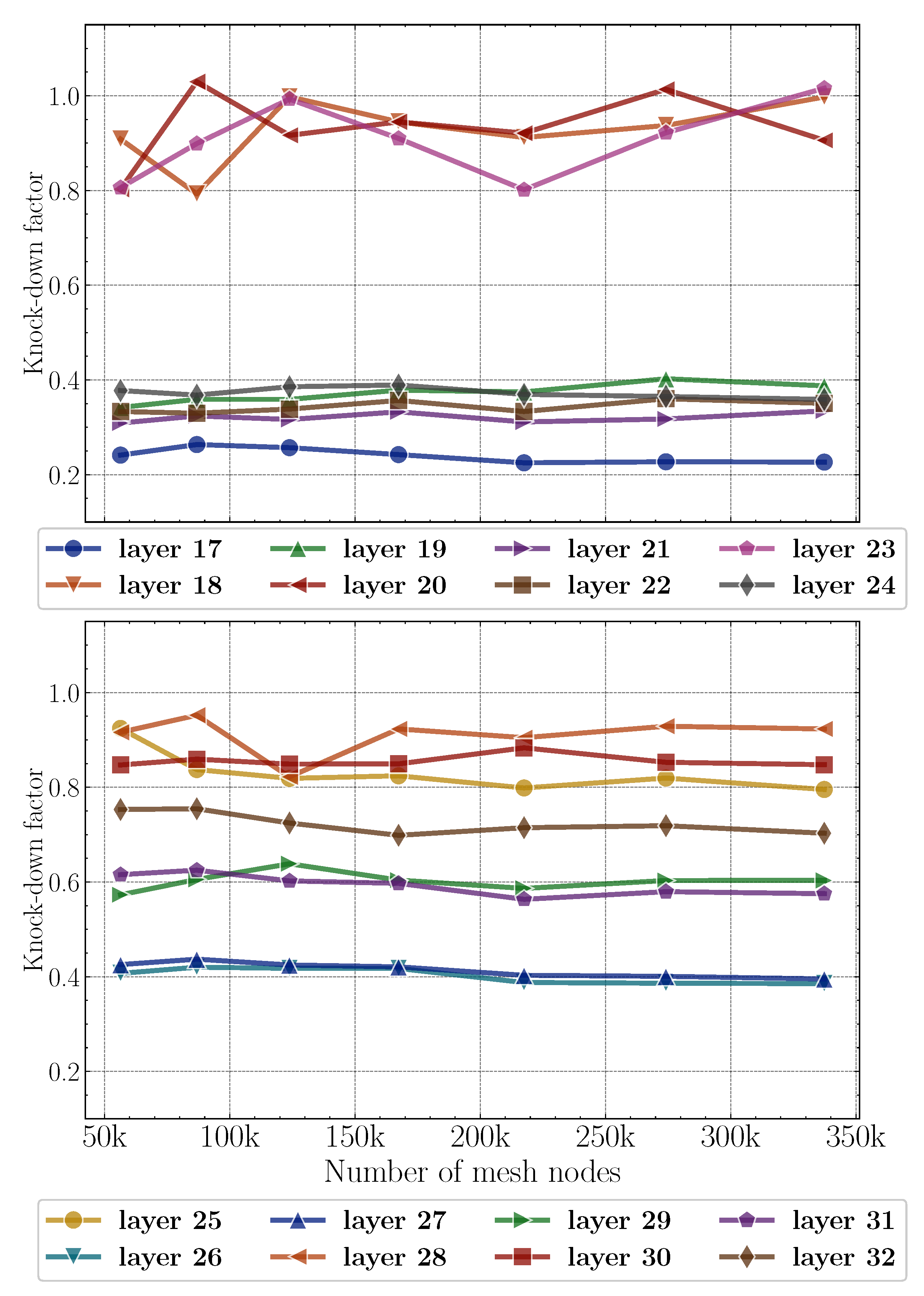
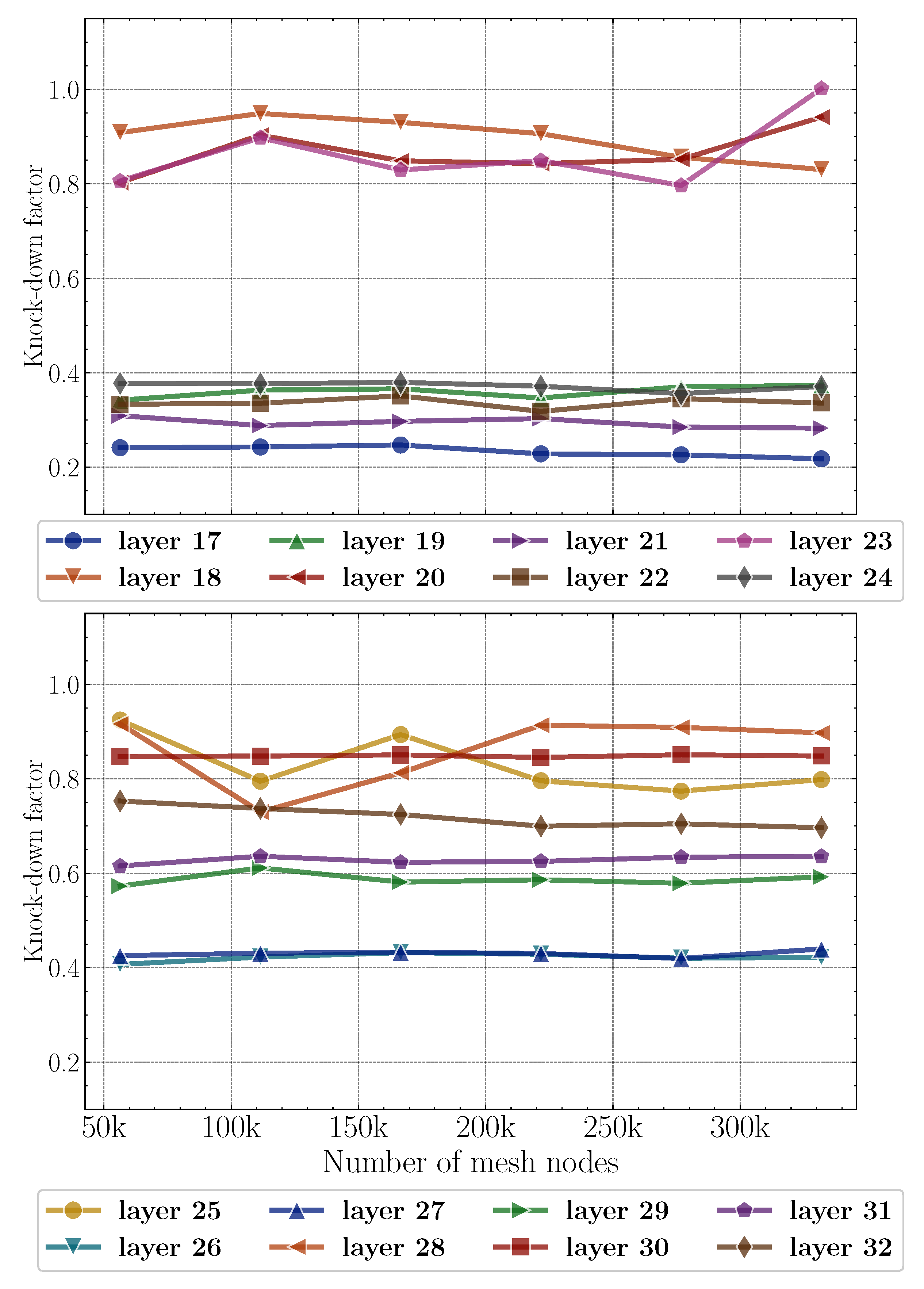
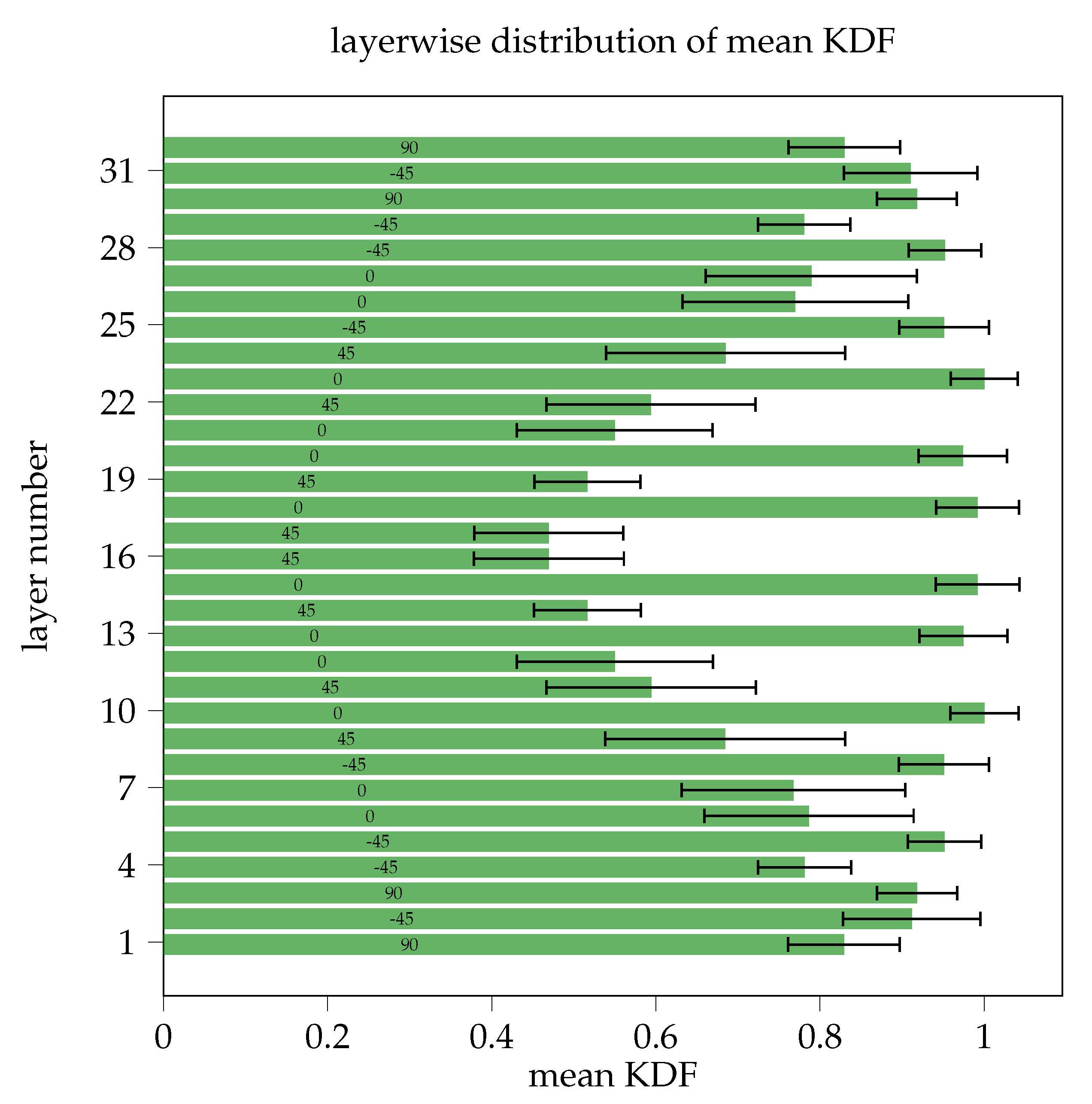
5.3.1. Statistical Distribution of KDF across Layers

Based on the deterministic results, the actual probabilistic analysis was done. Since the physical problem shows less sensitivity against the spatial resolution of the laminate model, a coarser mesh model was therefore selected which also reduces the computational effort in the stochastic procedure. To get statistically meaningful results, a huge number of independent samples need to be evaluated. As a random sampling algorithm, the Latin hypercube sampling method was used with 5000 samples in total. The number of input variables is equal to the number of decoupled standard normal distributions as a result of the KLE approach and was set to 50 in the stochastic analysis procedure. Figure 11 shows the mean-averaged KDF values of all samples with variance attached.

From Figure 11, a fully symmetric result with respect to the laminate center plane can be recognized, which was expected through the specific application of boundary conditions in the homogenization approach and applied loads as well as the chosen laminate stacking sequence. Complementary to Figure 9 and Figure 10, it can be seen that most plies with an orientation coincident with the load direction are not affected by undulations for a huge number of configurations due to a high mean KDF and low variance.

In Figure 12, the full histograms for each layer above the midsurface in the laminate are depicted. While the major fraction exhibits a normal or Weibull-like distribution, some of the plies show a complex dispersion of the KDF with a larger variance and a concentration of higher values approaching 1, which means no degradation. An initial analysis of the available results using the Puck failure criterion, which distinguishes between fiber and matrix fracture, indicates a complex failure mechanism. This is a crucial subject to be analyzed in future studies.

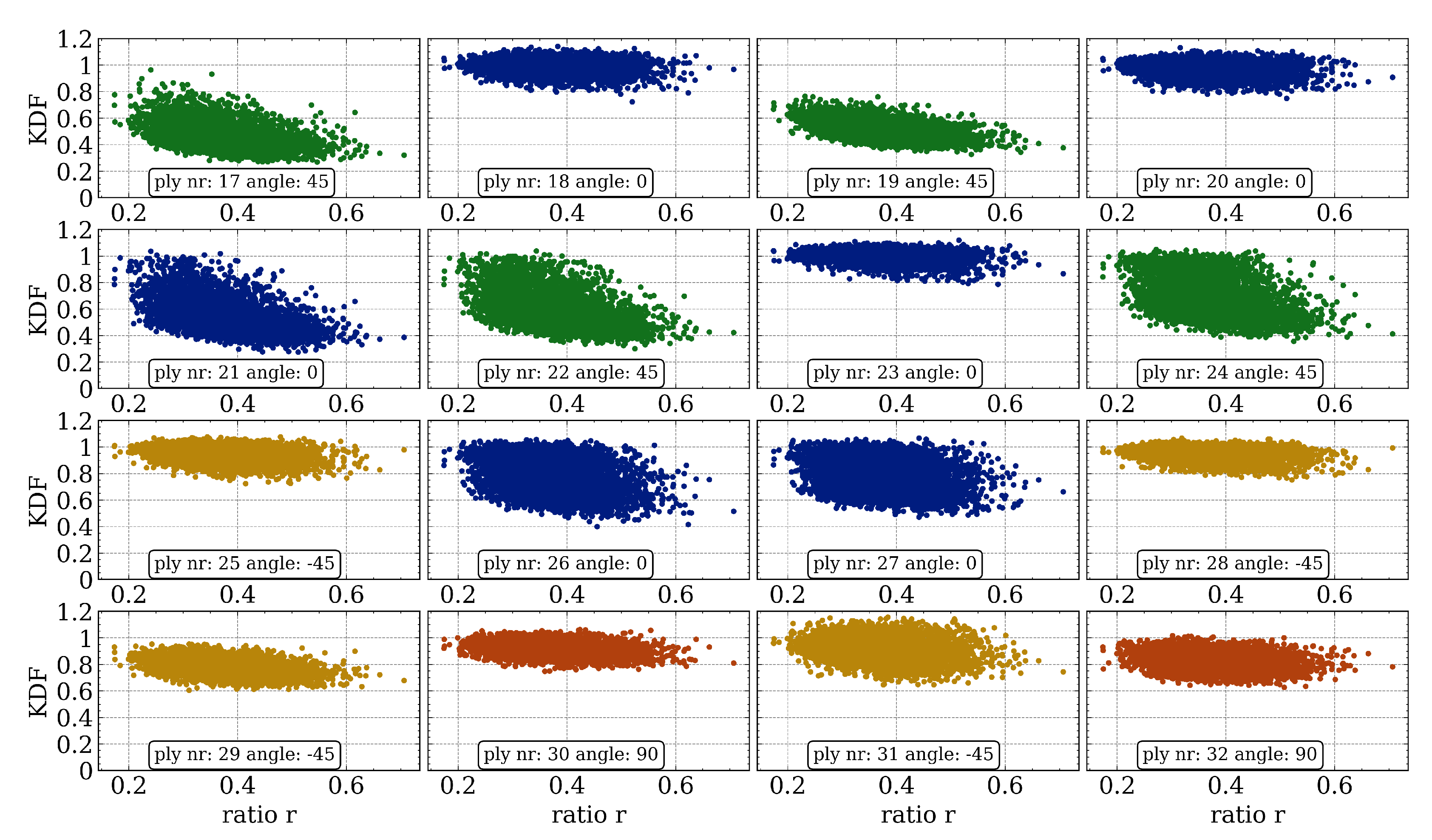
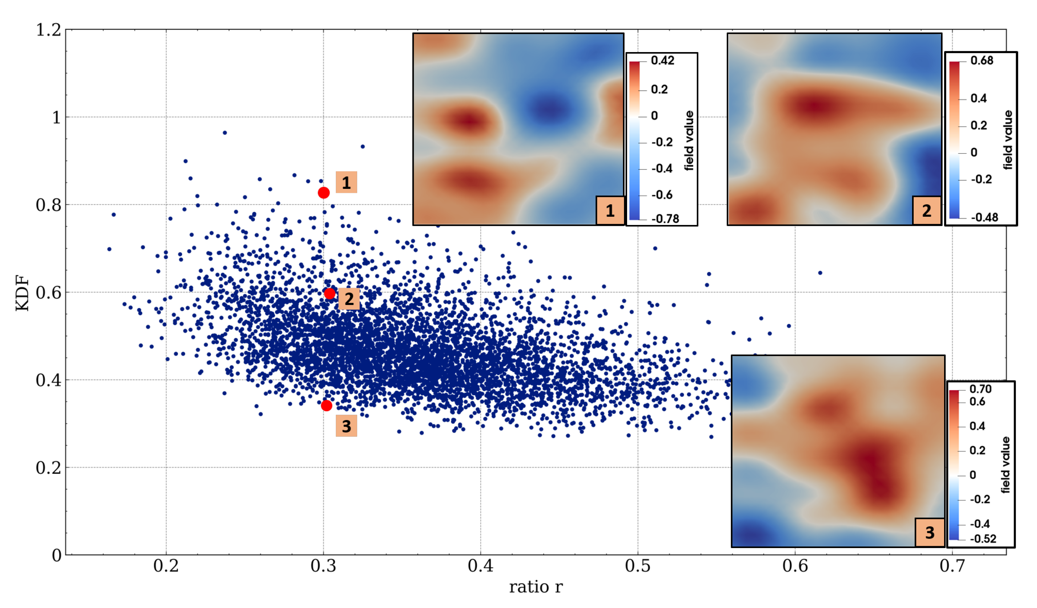
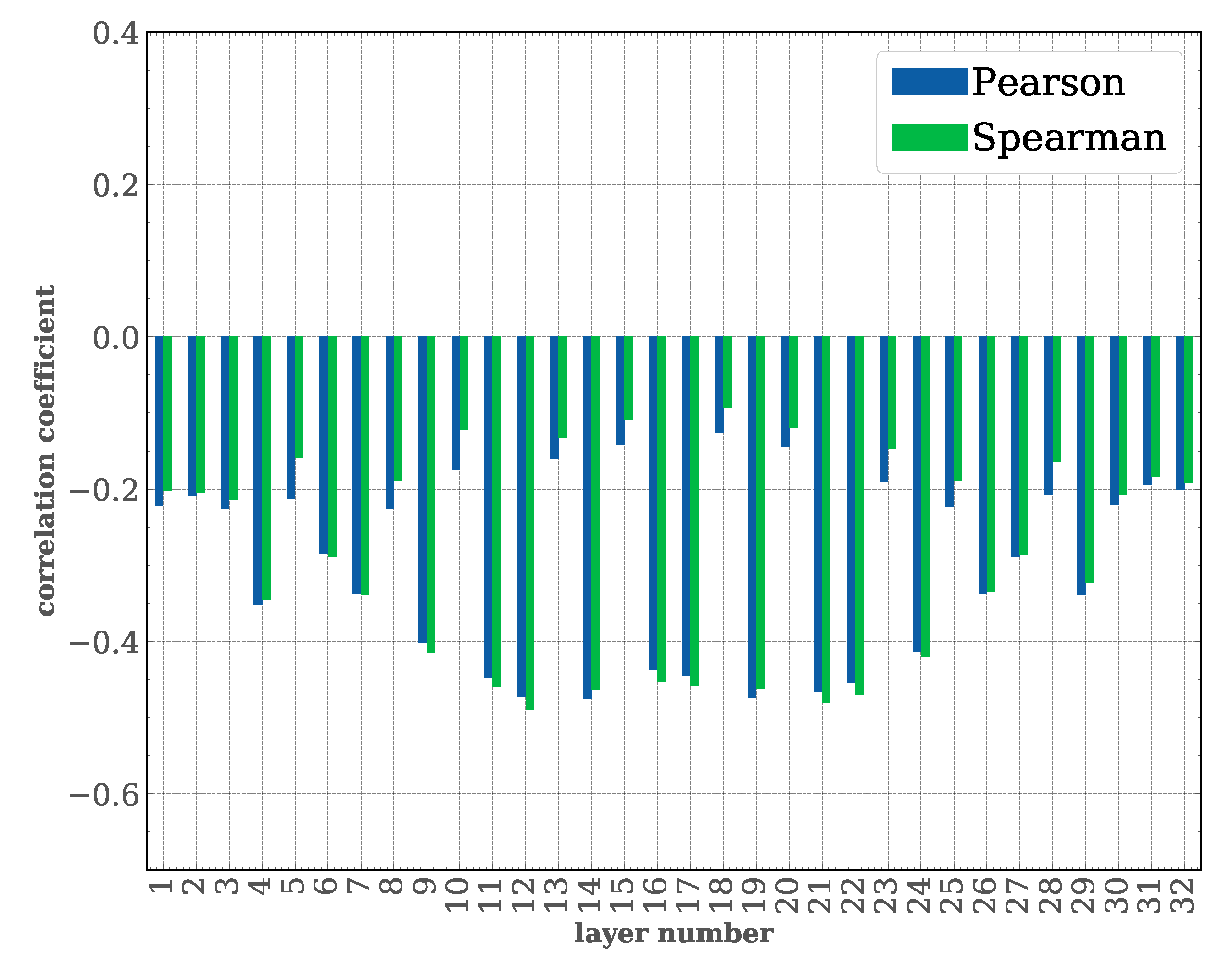
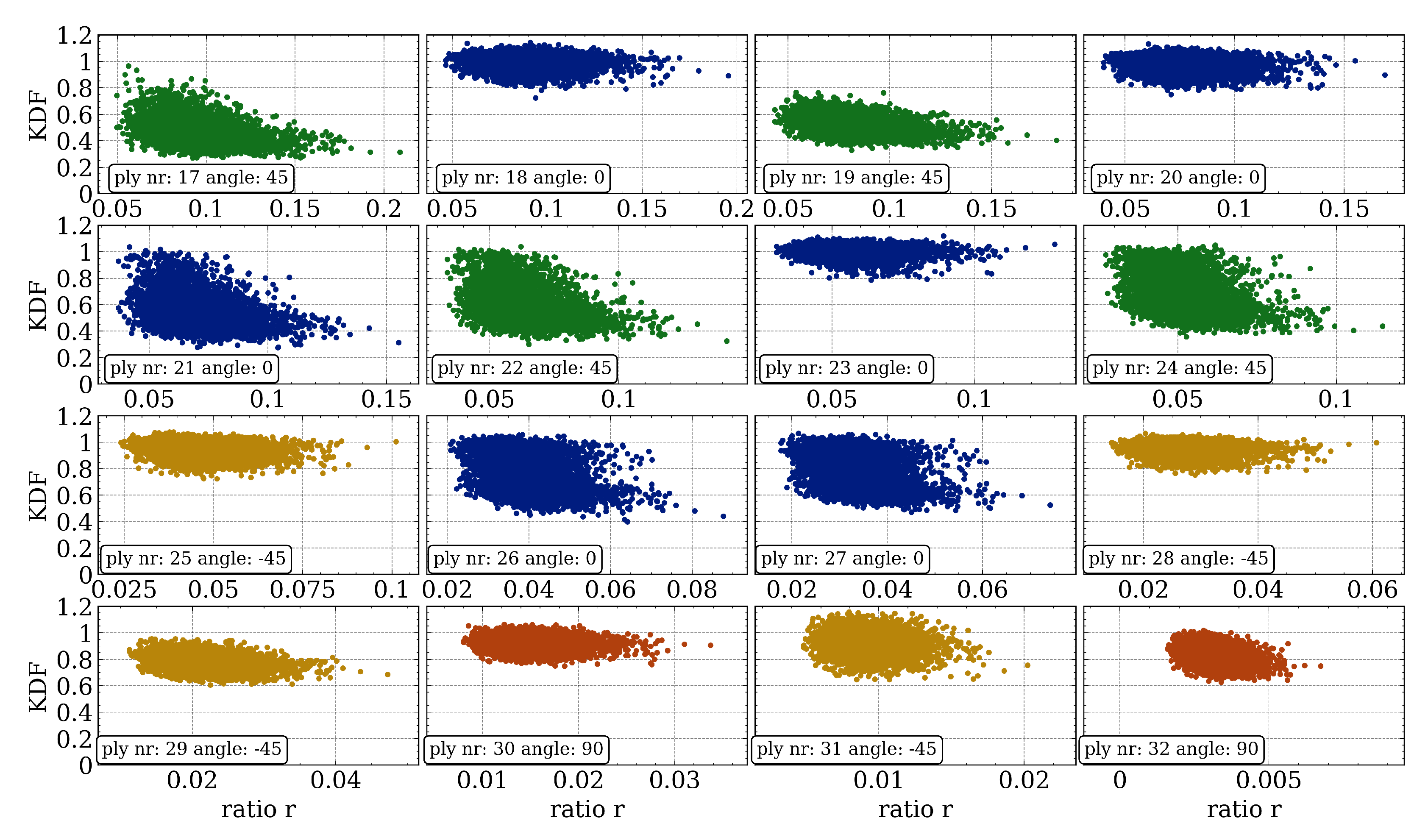
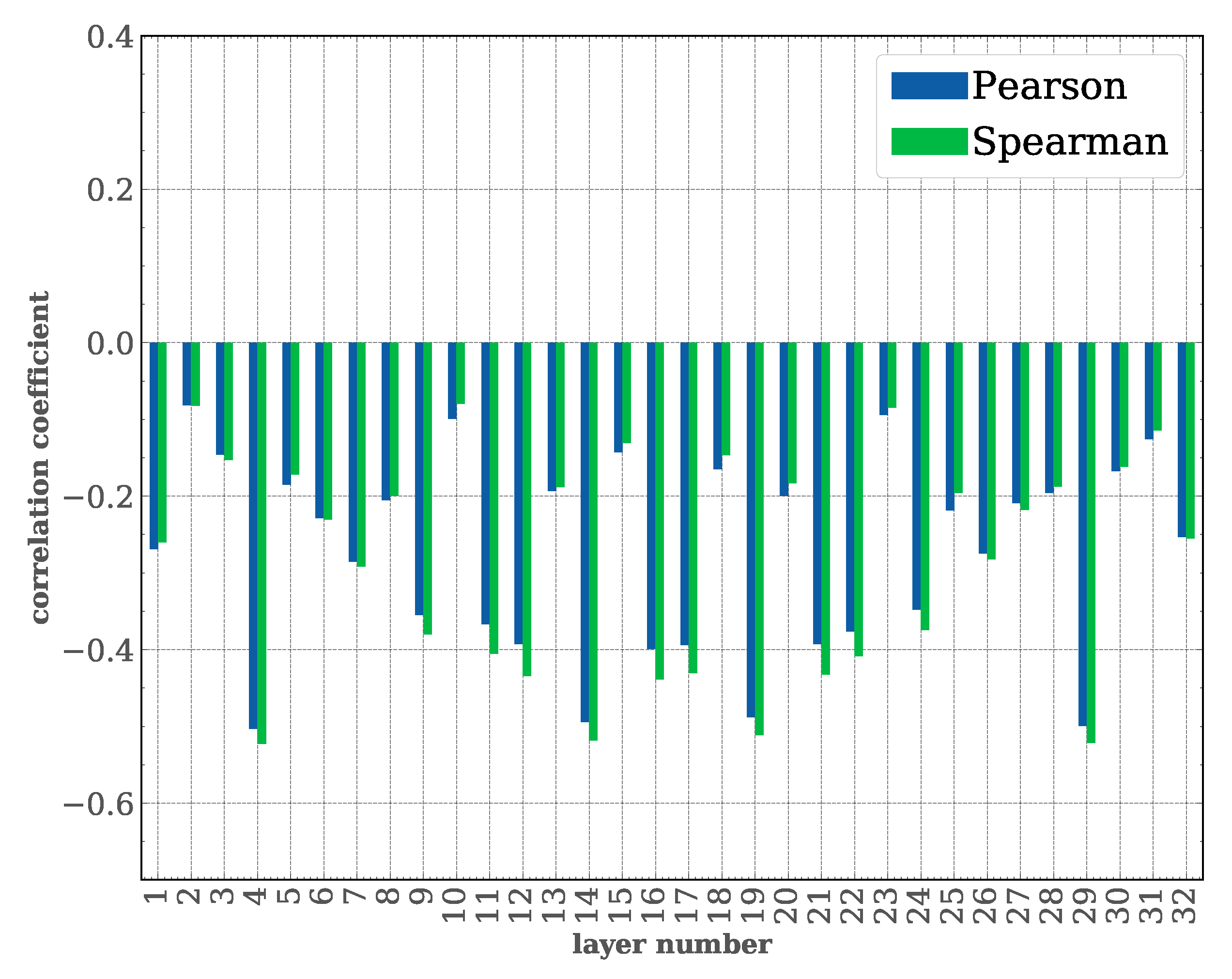
5.3.2. Relation between KDF and Waviness Parameters

Due to the limited expressiveness of the statistical results, it is of interest whether a simple parameter reduction of the complex waviness geometries is sufficient to describe the material behavior in a more comprehensible way. The reason for this is the assumption that failure initiation is closely related to large local gradients or amplitudes in the waviness geometry. Studies in the literature [11,17,19,49] already have shown such a relation for specific two-dimensional waviness parametrizations. However, the question arises if that approach can be easily transferred to the three-dimensional problem setting of this contribution. According to this issue, two exemplary metrics were selected for further consideration, and are evaluated on each ply:

(1)

Ratio of waviness amplitude to laminate thickness;

(2)

Maximum curvature in the fiber orientation direction.

It should be mentioned that the former metric is only evaluated once on the reference random field at the midsurface of the laminate, where the latter metric takes also the position of each ply in the laminate into account. Both metrics are evaluated for each random field sample in the probabilistic analysis study.

Ratio of Waviness Amplitude to Laminate Thickness

For the first selected metric, the maximum and minimum of the random field $H(x,\theta )$ are estimated. The distance between the minimum and maximum is then evaluated as the amplitude of the field. Compared to trigonometric waviness parametrization as frequently applied in the literature, where the amplitude is one of the input parameters of the model, the amplitude in a random waviness field can only be estimated at runtime. Fortunately, this does not lead to a large increase in run-time. After having the amplitude computed, it is scaled with the thickness $t_{lam}$ of the laminate, resulting in a value range between zero and one that is named in the following as ratio r:

$$r=\frac{max\left(H\right)-min\left(H\right)}{t_{lam}}$$

(13)

In Figure 13, the different KDFs for each ply dependent on the previously explained amplitude metric are plotted. For a better visual analysis, plies with the same orientation are colored accordingly. The computed ratios lie in the range between 0.173 and 0.706.

In addition, Figure 14 highlights three exemplary waviness field samples with an almost equal ratio ($r\approx 0.3$) but a huge difference in the resulting KDF at the midsurface ply in the laminate.

Without a claim of completeness, some first observations can be made from the figures:

• Only a minor ply fraction of the full laminate is subjected to a large decrease (>30 percent) of the KDF for higher waviness ratios.
• A large decrease of the KDF occurs only on plies with orientation angles of zero degrees and 45 degrees.
• For all different ply orientations except zero degrees, a similar result pattern (decreasing, constant within some range) can be observed.
• A large reduction due to a low KDF can already be identified for small to moderate waviness ratios ($0.2<r<0.3$).
• Even for moderate waviness ratios ($r\approx 0.4$) there is a large remaining scatter in the KDF for different random field samples between an unaffected resulting material behavior (KDF $\approx 1.0$) and a large degradation of the tensile strength property.

At this point, it should be mentioned that the observations only correspond to the selected laminate stacking sequence unless proven for other laminate configurations. For a different sequence, the results may be completely different.

To undergird these first visual inspections from a statistical point of view, correlation coefficients are derived from the scatter results. As representative methods, Spearman’s rank and Pearson’s correlation coefficients [50] are used to assess the relationship between the result variables. Figure 15 shows the correlation results for both selected coefficients.

From the figure, a weak correlation can be drawn for most of the KDFs for each ply within the laminate. On the other hand, the KDF of plies with an orientation angle of 45 degrees near the midsurface of the laminate exhibit a moderate correlation with a negative minimum of −0.49.

Maximum Curvature in Fiber Orientation Direction

In the second step, the maximum fiber curvature is analyzed as a metric. The determination is realized by an initial coordinate transformation of the discretized mesh of random field parallel to the fiber direction of each laminate ply and a numerical computation of the second derivative of the local field value by using a finite-difference approach. In Figure 16, the results for this metric are displayed. Compared with Figure 13, it shows similar results so that even for small curvatures in the waviness field, the resulting KDF lies in a larger range.

Finally, Figure 17 shows the results for the corresponding Spearman’s rank and Pearson’s correlation coefficients. Compared with the waviness amplitude metric, similar quantitative values can be recognized with a slightly larger maximum negative correlation coefficient of about −0.51.

Summary of the Metric Assessment

According to the results shown previously, no simplified relationships between the preselected metrics—amplitude-to-thickness ratio and maximum fiber curvature—as representative parameters for the stochastic waviness geometry and the resulting material properties described by the KDF can be inferred. The remaining scatter estimated from the results may, therefore, have further unknown manifold origins. One crucial aspect to be mentioned here is the choice of the Puck failure criterion, which might not be able to describe the complex material failure comprehensively. On the other hand, the large scatter can be accompanied by a higher-dimensional correlation structure in the result data induced by the complex geometrical pattern of the waviness field. For a proper assessment, sophisticated geometrical metrics would be required as part of a separate detailed analysis of the random field. Instead of maximum amplitude, all local extreme points may be taken into account, for instance. Yet, numerical gradient evaluations as key ingredients that seem to be reasonable for this purpose may suffer from robustness issues. A promising alternative approach is the so-called topological data analysis [51]. However, this hampers the ease of use of a spatial numerical defect assessment in industry-related scenarios, since this requires accurate measurement techniques to capture complex waviness formations in CFRP materials used for validation of the developed numerical approach.

6. Conclusions

This paper proposes a stochastic approach for the strength assessment of spatial out-of-plane fiber waviness defects in composite materials based on high-fidelity numerical models. The methodology relies on a homogenization approach at the laminate level, which is able to resolve the complex stress distribution due to fiber waviness. The stochastic waviness model relies on the Gaussian random field concept supplemented by a Karhunen–Loève expansion method as a numerical approximation. The proposed methodology and results contribute to deriving valid decisions in terms of repairing and inspection processes in future industrial scenarios applied to physically built composite structures. For a mature use in this context, intensive investigation on spatial distributions and amplitudes of waviness defects supported by optical measurement techniques are a key need that are the authors aware of. From a numerical point of view, different aspects need to be analyzed further. One crucial aspect is the analysis of the complex failure mechanism which led to a larger variance for partial result data, which was likely induced by the selected Puck failure criterion. For a robust derivation of the main failure aspects, different criteria for CFRP materials need to be analyzed additionally. Furthermore, there is still a huge computational effort to assess proper statistical properties for the considered material parameters, which is to be highlighted. Due to the high number of stochastic parameters, common surrogate models are likely to fail with the given input sample data and result distributions. Approaches such as [52] for use in higher dimensions may be promising candidates but need to be analyzed in detail in the potential nonlinear context of this contribution.

Regardless of the accuracy of such types of surrogate models, sampling methods used for input generation in the stochastic analysis are only able to cover a small fraction of the possible parameter space due to the time-consuming FEM-based evaluation process and finite computational resources. Analytical methods to efficiently compute the stress distribution within orthotropic CFRP materials are an essential key for the efficient use of the spatial stochastic model. However, such approaches still do not exist for use in a generic three-dimensional physical problem such as the one analyzed in this paper. Therefore, the determination of large real-world inspection data as stochastic input still remains a necessary step for proper and efficient use of stochastic numerical analysis in assessment processes of manufacturing-induced material defects. The same also holds for the validation of the achieved numerical results based on a suitable experimental strength assessment.

References

1. Heinecke, F.; Willberg, C. Manufacturing-Induced Imperfections in Composite Parts Manufactured via Automated Fiber Placement. J. Compos. Sci. 2019, 3, 56. [Google Scholar] [CrossRef] [Green Version]
2. Hallander, P.; Akermo, M.; Mattei, C.; Petersson, M.; Nyman, T. An experimental study of mechanisms behind wrinkle development during forming of composite laminates. Compos. Part A Appl. Sci. Manuf. 2013, 50, 54–64. [Google Scholar] [CrossRef]
3. Krämer, E.; Grouve, W.; Koussios, S.; Warnet, L.L.; Akkerman, R. Real-time observation of waviness formation during C/PEEK consolidation. Compos. Part A Appl. Sci. Manuf. 2020, 133, 105872. [Google Scholar] [CrossRef]
4. Thor, M.; Sause, M.G.R.; Hinterhölzl, R.M. Mechanisms of Origin and Classification of Out-of-Plane Fiber Waviness in Composite Materials—A Review. J. Compos. Sci. 2020, 4, 130. [Google Scholar] [CrossRef]
5. Mukhopadhyay, S.; Jones, M.I.; Hallett, S.R. Modelling of out-of-plane fibre waviness; tension and compression tests. In Proceedings of the 4th ECCOMAS Thematic Conf. on the Mechanical Response of Composites, Saint Miguel, Portugal, 25–27 September 2013; pp. 17–22. [Google Scholar]
6. Davidson, P.; Waas, A.; Yerramalli, C.; Chandraseker, K.; Faidi, W. Effect of Fiber Waviness on the Compressive Strength of Unidirectional Carbon Composites. In Proceedings of the 53rd AIAA/ASME/ASCE/AHS/ASC Structures, Structural Dynamics and Materials Conference, Honolulu, Hawaii, 23–26 April 2012. [Google Scholar] [CrossRef] [Green Version]
7. Hinterhölzl, R.M.; Haller, H.; Luger, M.; Klar, R. Strategy for a simulation based assessment of effects of manufacturing. In Proceedings of the 5th International Conference Supply Wings Airtech, Frankfurt, Germany, 2–4 November 2010. [Google Scholar]
8. Tarnopol’skii, Y.M.; Portnov, G.G.; Zhigun, I.G. Effect of fiber curvature on the modulus of elasticity for unidirectional glass-reinforced plastics in tension. Polym. Mech. 1971, 3, 161–166. [Google Scholar] [CrossRef]
9. Hsiao, H.M.; Daniel, I.M. Effect of fiber waviness on stiffness and strength reduction of unidirectional composites under compressive loading. Compos. Sci. Technol. 1996, 56, 581–593. [Google Scholar] [CrossRef]
10. Piggott, M.R. The effect of fibre waviness on the mechanical properties of unidirectional fibre composites: A review. Compos. Sci. Technol. 1995, 53, 201–205. [Google Scholar] [CrossRef]
11. Thor, M.; Mandel, U.; Nagler, M.; Maier, F.; Tauchner, J.; Sause, M.G.R.; Hinterhölzl, R.M. Numerical and experimental investigation of out-of-plane fiber waviness on the mechanical properties of composite materials. Int. J. Mater. Form. 2021, 14, 19–37. [Google Scholar] [CrossRef] [Green Version]
12. Heinecke, F.; Wille, T. In-situ structural evaluation during the fibre deposition process of composite manufacturing. CEAS Aeronaut. J. 2018, 9, 123–133. [Google Scholar] [CrossRef]
13. Willberg, C.; Heinecke, F. Evaluation of manufacturing deviations of composite materials. PAMM 2021, 20, e202000345. [Google Scholar] [CrossRef]
14. Al-kathemi, N.; Wille, T.; Heinecke, F.; Degenhardt, R.; Wiedemann, M. Interaction effect of out of plane waviness and impact damages on composite structures—An experimental study. Compos. Struct. 2021, 276, 114405. [Google Scholar] [CrossRef]
15. Khattab, I.A.d.; Kreikemeier, J.; Abdelhadi, N.S. Manufacturing of CFRP specimens with controlled out-of-plane waviness. CEAS Aeronaut. J. 2014, 5, 85–93. [Google Scholar] [CrossRef]
16. Adams, D.O.; Bell, S.J. Compression strength reductions in composite laminates due to multiple-layer waviness. Compos. Sci. Technol. 1995, 53, 207–212. [Google Scholar] [CrossRef]
17. Elhajjar, R.F.; Shams, S.S. Compression testing of continuous fiber reinforced polymer composites with out-of-plane fiber waviness and circular notches. Polym. Test. 2014, 35, 45–55. [Google Scholar] [CrossRef]
18. Sutton, M.A.; Orteu, J.J.; Schreier, H.W. Image Correlation for Shape, Motion and Deformation Measurements: Basic Concepts, Theory and Applications; Springer: New York, NY, USA, 2009. [Google Scholar]
19. Sandhu, A.; Reinarz, A.; Dodwell, T.J. A Bayesian framework for assessing the strength distribution of composite structures with random defects. Compos. Struct. 2018, 205, 58–68. [Google Scholar] [CrossRef] [Green Version]
20. Kriegesmann, B.; Balokas, G.; Wille, T. Uncertainty quantification of composite structures with manufacturing defects within the SuCoHS project. In Proceedings of the 8th European Congress on Computational Methods in Applied Sciences and Engineering (ECCOMAS 2022), Oslo, Norway, 5–9 June 2022. [Google Scholar]
21. Arai, Y.; Fukuda, K.; Sakata, S.i. Random Field Modeling of Microstructure in Unidirectional Fiber–Reinforced Plastic Using SEM–Image and Image Processing for Multiscale Stochastic Stress Analysis Considering Random Fiber Arrangements. Adv. Eng. Mater. 2022, 24, 2270020. [Google Scholar] [CrossRef]
22. Rauter, N. A computational modeling approach based on random fields for short fiber-reinforced composites with experimental verification by nanoindentation and tensile tests. Comput. Mech. 2021, 67, 699–722. [Google Scholar] [CrossRef]
23. Machina, G.; Zehn, M.W. A methodology to model spatially distributed uncertainties in thin-walled structures. ZAMM 2007, 87, 360–376. [Google Scholar] [CrossRef]
24. Zein, S.; Laurent, A.; Dumas, D. Simulation of a Gaussian random field over a 3D surface for the uncertainty quantification in the composite structures. Comput. Mech. 2019, 63, 1083–1090. [Google Scholar] [CrossRef]
25. Kepple, J.; Herath, M.T.; Pearce, G.; Gangadhara Prusty, B.; Thomson, R.; Degenhardt, R. Stochastic analysis of imperfection sensitive unstiffened composite cylinders using realistic imperfection models. Compos. Struct. 2015, 126, 159–173. [Google Scholar] [CrossRef]
26. Dodwell, T.J.; Kinston, S.; Butler, R.; Haftka, R.T.; Kim, N.H.; Scheichl, R. Multilevel Monte Carlo Simulations of Composite Structures with Uncertain Manufacturing Defects. Probabilistic Eng. Mech. 2021, 63, 103116. [Google Scholar] [CrossRef]
27. Sutcliffe, M. Modelling the effect of size on compressive strength of fibre composites with random waviness. Compos. Sci. Technol. 2013, 88, 142–150. [Google Scholar] [CrossRef]
28. Sutcliffe, M.; Lemanski, S.L.; Scott, A.E. Measurement of fibre waviness in industrial composite components. Compos. Sci. Technol. 2012, 72, 2016–2023. [Google Scholar] [CrossRef] [Green Version]
29. Heinecke, F. Strukturmechanische Auswirkung fertigungsbedingter Imperfektionen aus Faserverbundablegeprozesses. Ph.D. Thesis, Technische Universität Carola-Wilhelmina zu Braunschweig, Brunswick, Germany, 2020. [Google Scholar]
30. Puck, A. Festigkeitsanalyse von Faser-Matrix-Laminaten: Modelle für die Praxis (Trength Analysis of Fibre-Matrix/Laminates, Models for Design Practice); Hanser: Munich, Germany; Vienna, Austria, 1996. [Google Scholar]
31. Liu, K. A progressive quadratic failure criterion for a laminate. Compos. Sci. Technol. 1998, 58, 1023–1032. [Google Scholar] [CrossRef]
32. Kolios, A.J.; Proia, S. Evaluation of the Reliability Performance of Failure Criteria for Composite Structures. World J. Mech. 2012, 2, 162–170. [Google Scholar] [CrossRef] [Green Version]
33. Bogetti, T.A.; Gillespie, J.W.; Lamontia, M.A. Influence of Ply Waviness on the Stiffness and Strength Reduction on Composite Laminates. J. Thermoplast. Compos. Mater. 1992, 5, 344–369. [Google Scholar] [CrossRef]
34. Karami, G.; Garnich, M. Effective moduli and failure considerations for composites with periodic fiber waviness. Compos. Struct. 2005, 67, 461–475. [Google Scholar] [CrossRef]
35. Gichman, I.I.; Skorochod, A.V. Introduction to the Theory of Random Processes; Dover Books on Mathematics; Dover Publications: Mineola, NY, USA, 1996. [Google Scholar]
36. Reinarz, A.; Dodwell, T.; Fletcher, T.; Seelinger, L.; Butler, R.; Scheichl, R. Dune-composites—A new framework for high-performance finite element modelling of laminates. Compos. Struct. 2018, 184, 269–278. [Google Scholar] [CrossRef]
37. Karhunen, K. Über lineare Methoden in der Wahrscheinlichkeitsrechnung; Annales Academiae Scientiarum Fennicae: Ser. A 1; Universitat Helsinki: Helsinki, Finland, 1947. [Google Scholar]
38. Betz, W.; Papaioannou, I.; Straub, D. Numerical methods for the discretization of random fields by means of the Karhunen–Loève expansion. Comput. Methods Appl. Mech. Eng. 2014, 271, 109–129. [Google Scholar] [CrossRef]
39. Stefanou, G. The stochastic finite element method: Past, present and future. Comput. Methods Appl. Mech. Eng. 2009, 198, 1031–1051. [Google Scholar] [CrossRef] [Green Version]
40. Schuëller, G.I. Developments in stochastic structural mechanics. Arch. Appl. Mech. 2006, 75, 755–773. [Google Scholar] [CrossRef]
41. Bathe, K.J. Finite-Elemente-Methoden; Springer: Berlin/Heidelberg, Germany, 2002. [Google Scholar]
42. Geuzaine, C.; Remacle, J.F. Gmsh: A 3-D finite element mesh generator with built-in pre- and post-processing facilities. Int. J. Numer. Methods Eng. 2009, 79, 1309–1331. [Google Scholar] [CrossRef]
43. SMR. B2000++ Finite Element Analysis Environment. Available online: https://www.smr.ch/products/b2000 (accessed on 30 September 2022).
44. Kaddour, A.S.; Hinton, M.J. Input data for test cases used in benchmarking triaxial failure theories of composites. J. Compos. Mater. 2012, 46, 2295–2312. [Google Scholar] [CrossRef]
45. Wunderlich, T.F.; Dähne, S.; Reimer, L.; Schuster, A. Global aero-structural design optimization of composite wings with active manoeuvre load alleviation. CEAS Aeronaut. J. 2022, 13, 639–662. [Google Scholar] [CrossRef]
46. Dillinger, J. Static Aeroelastic Optimization of Composite Wings with Variable Stiffness Laminate. Ph.D. Thesis, Delft University of Technology, Delft, The Netherlands, 2014. [Google Scholar] [CrossRef]
47. Baudin, M.; Dutfoy, A.; Iooss, B.; Popelin, A.L. OpenTURNS: An Industrial Software for Uncertainty Quantification in Simulation. In Handbook of Uncertainty Quantification; Ghanem, R., Higdon, D., Owhadi, H., Eds.; Springer eBook Collection; Springer: Cham, Switzerland, 2017; pp. 1–38. [Google Scholar] [CrossRef] [Green Version]
48. McKay, M.D.; Beckman, R.J.; Conover, W.J. A Comparison of Three Methods for Selecting Values of Input Variables in the Analysis of Output from a Computer Code. Technometrics 1979, 21, 239. [Google Scholar] [CrossRef]
49. O’Hare Adams, D.; Hyer, M.W. Effects of Layer Waviness on the Compression Strength of Thermoplastic Composite Laminates. J. Reinf. Plast. Compos. 1993, 12, 414–429. [Google Scholar] [CrossRef]
50. Weaver, K.F.; Morales, V.C.; Dunn, S.L. An Introduction to Statistical Analysis in Research: With Applications in the Biological and Life Sciences; John Wiley & Sons Inc: Hoboken, NJ, USA, 2018. [Google Scholar] [CrossRef]
51. Edelsbrunner; Letscher; Zomorodian. Topological Persistence and Simplification. Discret. Comput. Geom. 2002, 28, 511–533. [Google Scholar] [CrossRef] [Green Version]
52. Papaioannou, I.; Ehre, M.; Straub, D. PLS-based adaptation for efficient PCE representation in high dimensions. J. Comput. Phys. 2019, 387, 186–204. [Google Scholar] [CrossRef]
Figure 1. Two-dimensional examples of out-of-plane fiber waviness in a composite laminate. (a) Embedded single graded waviness, reprinted with permission from Ref. [5], 2013, S. Mukhopadhyay; (b) hump, reprinted with permission from Ref. [6], 2012, P. Davidson; (c) complex stochastic distributed waviness, reprinted with permission from Ref. [7], 2010, R. Hinterhölzl.
Jcs 06 00353 g001
Figure 2. Illustration of homogenization approach for KDF parameter estimation based on pristine (left) and defective model configuration (right), reprinted with permission from Ref. [29], 2020, F. Heinecke).
Jcs 06 00353 g002
Figure 3. Exemplary Matern-kernel functions for the different realization of the parameter ν .
Jcs 06 00353 g003
Figure 4. KLE-based waviness modeling of a generic CFRP cross-section made up of 8 layers for three different numbers of eigenvalues. The numerical approximated random field is highlighted in red. (a) 6 modes; (b) 12 modes; (c) 20 modes.
Jcs 06 00353 g004
Figure 5. Simplified workflow for the estimation of stochastic knock-down factors.
Jcs 06 00353 g005
Figure 6. Two examples of random field realizations embedded in a reference FE model for a laminate of the thickness t l a m with about 169,000 degrees of freedom. The upper half layers of the laminate are made transparent for visibility. The color indicates the relative displacements of the ply with respect to a nominal pristine position.
Jcs 06 00353 g006
Figure 7. Node sets at model boundary and applied loads for tensile loadcase. (Reprinted with permission from Ref. [29], 2020, F. Heinecke).
Jcs 06 00353 g007
Figure 8. (a) KDF plot of deterministic analysis for R x loadcase; (b) random field example used for deterministic analysis.
Jcs 06 00353 g008
Figure 9. Convergence of KDF according to mesh refinement in the x-direction.
Jcs 06 00353 g009
Figure 10. Convergence of KDF according to mesh refinement in the z-direction (layer thickness direction).
Jcs 06 00353 g010
Figure 11. Distribution of mean of KDF for R x within the selected laminate configuration with related variances as second bar element of the stochastic results. For each layer, the ply angle is additionally printed.
Jcs 06 00353 g011
Figure 12. Distribution of KDF histograms for R x at specific layers within selected laminate configuration.
Jcs 06 00353 g012
Figure 13. Scatter plot of waviness ratio compared to resulting KDF for property R x . Plies that share the same fiber orientation angle are colored equally.
Jcs 06 00353 g013
Figure 14. Selection of three exemplary random fields with a similar waviness ratio at the midsurface of the laminate.
Jcs 06 00353 g014
Figure 15. Correlation coefficients for tensile KDF related to waviness ratio.
Jcs 06 00353 g015
Figure 16. Scatter plot of maximum curvature in fiber orientation direction compared to resulting KDF for R x . Plies that share the same fiber orientation angle are colored equally.
Jcs 06 00353 g016
Figure 17. Correlation coefficient for tensile KDF related to fiber orientation aligned maximum curvature.
Jcs 06 00353 g017