Applicability of Asymmetric Specimens for Residual Stress Evaluation in Fiber Metal Laminates

Abstract

Residual stresses in fiber metal laminates (FML) inevitably develop during the manufacturing process. The main contributor to these stresses is the difference in the coefficients of thermal expansion (CTE) between fibers and metal in combination with high process temperatures. To quantify these stresses, the use of specimens with an asymmetric layup is an easily adaptable method. The curvature that develops after the manufacturing of flat laminates with an asymmetrical layer stack is a measure of the level of residual stresses evolving during cure. However, the accuracy of the curvature evaluation is highly dependent on specimen design and other influencing parameters. This leads to deviations when compared to other methods for residual stress quantification as can be seen from the literature. Therefore, in this work a large set of FML specimens is comprehensively investigated to identify relevant influencing parameters and derive conclusions about specimen design and evaluation techniques. For certain layups and process parameters, there is a good correlation between the curvature and the stress-free temperature, which is further covered by analytical solutions for bimetals. This correlation is the basis to transfer curvature into a stress-free temperature that can consequently be used for the quantification of residual stress levels in more complex FMLs. The transfer is validated by in situ strain measurements during cure using a strain gauge technique. Based on the results, the application of asymmetric specimens for residual stress characterization in more complex laminates is presented in the form of a workflow. The work shows the basic considerations and procedures necessary to use asymmetric specimens for residual stress quantification in FML. Furthermore, the results obtained can also be transferred to other composite materials.

1. Introduction

Fiber metal laminates (FML) are an advanced intrinsic hybrid material made from composites and metals [1]. FMLs are specifically designed for applications that would not be feasible with monolithic materials alone. The most prominent FML material arose from the goal of improving conventional aluminum for aerospace applications by laminating layers of glass-fiber-reinforced polymer together with thin sheets of aluminum. The result is a glass-fiber-reinforced aluminum (GLARE) that possesses superior damage tolerance and fatigue behavior compared to structures made from monolithic aluminum [2]. In contrast, applications evolved where the properties of monolithic composite materials are improved by reinforcing the material with thin metal sheets (mainly titanium and steel), for example, for load introduction zones [3], crash elements [4] or erosion protection [5].

However, residual stresses arise in the manufacturing process due to the different coefficients of thermal expansion (CTE) and the high stiffness of fibers and metal combined with high temperatures during manufacturing [6,7]. These stresses can lead to early component failure and act as damage initiators during fatigue loading [8]. The residual stresses can account for around 20% of the material strength dependent on the material combination, layup, and operating temperature [9,10]. Hence, it is obvious that residual stresses should be considered during the design process of FML structures.

For this purpose, the residual stress level in a manufactured component must be reliably quantified, for which a variety of methods exists in the literature. Based on [6], these can be divided into destructive and non-destructive methods, as well as methods that monitor the strains during the manufacturing process and those which try to make conclusions about the internal stress state of a specimen after manufacturing. The most accurate methods certainly are integrated or applied sensors that are capable of measuring the strains in situ during the manufacturing process. Recently, mainly fiber optic sensors (FOS), especially fiber Bragg grating (FBG) sensors (e.g., [11,12,13]), as well as strain gauges (e.g., [9,14]) were used in the literature.

The disadvantage of these sensors is the complex experimental setup, which is not suitable for continuous monitoring during industrial manufacturing processes. The curvature measurement, instead, seems to be a great option for industrial applications since the complexity during manufacturing is low, and the evaluation process can be transferred to the time after manufacturing. This method is also very prominent in the literature, e.g., [15,16,17] to determine the residual stresses developing in thermoplastic and thermoset carbon-fiber-reinforced composites. Beyond these investigations, [18] already used the curvature analysis for asymmetric FML specimens. In [6], however, it is stated that warpage or curvature measurements go along with limited accuracy of the results. Likewise, in [18] different evaluated parameters of curved laminates (curvature and stress-free temperature) show large deviations among themselves. It is assumed that the layup, laminate thickness, and dimensions of the specimens play a great role in terms of evaluation reliability besides the manufacturing process itself.

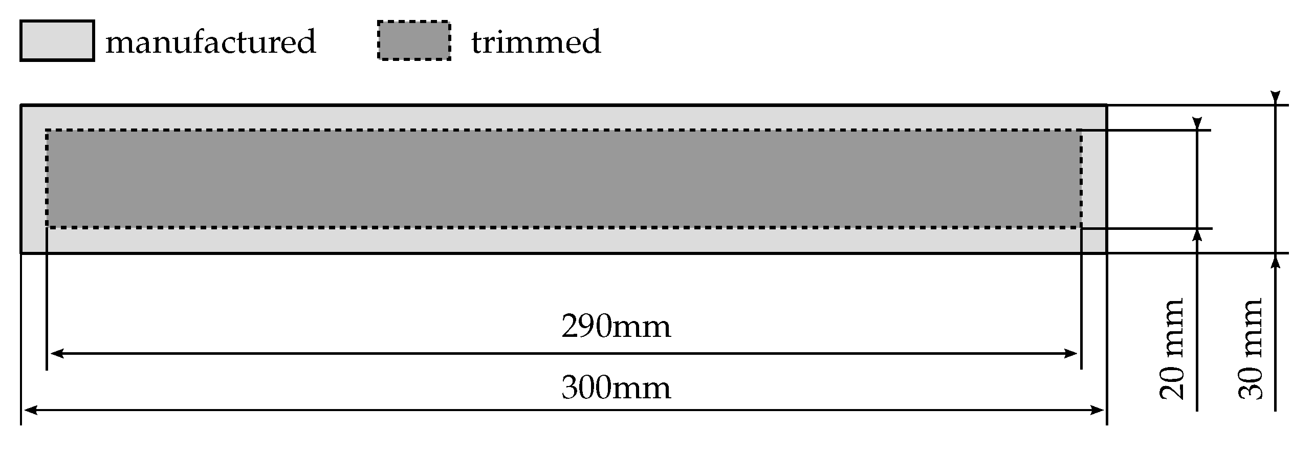
To see an overview of specimen dimensions and layups that were used in the literature,

Table 1. Asymmetric specimens made of carbon-fiber-reinforced polymer (CFRP) or fiber metal laminates (FML) used in the literature vary greatly in their dimensions and laminate layups.

Material	Source	Dimensions [mm2]	Width-to-Length Ratio	Layup	Thickness [mm]
CFRP	[20]	25 × 152	0.16	$0_3/{90}_3$	0.75
CFRP	[16]	100 × 230 ${}^{\mathrm{a}}$	0.4	$0/90$	0.25
CFRP	[15]	25/11 × 152	0.16/0.07	$0_4/{90}_4$	-
CFRP	[17]	25 × 150	0.16	${90}_4/0_2$, ${90}_2/0_2$, ${90}_2/0$	0.4–0.8
FML	[18]	20 × 200	0.1	$St/0$	0.25
FML	[13]	100 × 200	0.5	$St/0_3$	0.5
FML	This work	20 × 290 ${}^{\mathrm{a}}$	0.07	cf. Table 7	0.5–1.0

^a trimmed.

lists some sources with their corresponding asymmetric specimen architectures made of monolithic carbon-fiber-reinforced polymer (CFRP) or FML. The size of the specimens and the layups vary greatly. For small aspect ratios (width-to-length), the curvature in the transverse direction only influences the main curvature to a minor degree. With aspect ratios close to one, a saddle-shape curvature or a bi-stable deflection behavior is expected [17,19]. Therefore a width-to-length ratio of 0.07 is chosen in this work, whereas different layups and consequent laminate thicknesses are evaluated.

Asymmetric laminates can not only be investigated in terms of curvature but also their stress-free temperature $T_{sf}$ can be analyzed, e.g., [21,22,23]. The $T_{sf}$ is determined as that temperature at which curved laminates transition back into their initial plane state. Most of the time, the $T_{sf}$ is somewhere below the final cure temperature of the laminate [24,25]. The $T_{sf}$ is the relevant parameter when manufacturing-induced thermo-mechanical stresses need to be calculated in a laminate. Therefore, stress-free temperatures will likewise be evaluated in this work and correlated to measured curvatures using analytical and numerical methods.

Both parameters, curvature and stress-free temperature, are sensitive to several influencing factors that contribute to the residual stress state. These factors can generally be divided into intrinsic and extrinsic parameters [26,27]. Intrinsic parameters include material and layup-dependent anisotropy, whereas extrinsic parameters include tool and process influences. Although the different parameters are mainly investigated for monolithic FRP materials, the results can be equally transferred to FMLs. For FMLs however, the intrinsic anisotropy due to large differences in the coefficients of thermal expansion of the single constituents plays a greater role than for monolithic FRP.

The tool is a main extrinsic parameter affecting the residual stress state which mainly results from incompatibility in thermal expansion between tool and laminate. Two phenomena are differentiated in the literature, which are forced interaction [27,28] and warpage [27,29]. Since the laminates are manufactured in a plane state, no geometrical interlocking between the tool and composite part is present. Therefore, only the effect of warpage needs to be considered. Warpage mainly occurs for thin laminate thicknesses ($t\le 1\mathrm{m}\mathrm{m}$) in combination with large CTE differences between tool material and laminate [26]. Table 1 shows that the specimen architectures of the asymmetric specimens used in the literature are within the relevant thickness range for warpage; hence, this effect needs to be considered during the evaluation.

The other extrinsic parameter of interest is the cure cycle itself. It was shown that residual stress levels in a composite laminate can be directly influenced by modifying the temperature profile during cure [30,31,32,33]. The idea behind these modified cure cycles for thermoset resins is the shift of the gel point of the resin to a temperature as close as possible to room or operating temperature. By integrating intermediate cooling steps into the cure cycle, this can be achieved, and consequently thermal residual stresses can be reduced.

The range of influences shows that a comprehensive understanding of the effect of the different parameters on the residual stress state and hence on the curvature of an asymmetric specimen is necessary to develop a reliable method that uses curvature analysis for process monitoring and for residual stress quantification.

The general objective of this work is to describe a method that uses information from simple asymmetric laminates to determine the residual stress state in a more complex FML structure. The methodology should be easy to apply and provide good repeatable results. For this purpose, the influence of various relevant parameters on the curvature of asymmetric specimens is investigated, and recommendations for specimen design are given.

Section 2 explains all the relevant methods used in this work and introduces the materials and specimen manufacturing process. Subsequently, intrinsic and extrinsic parameters and their influence on the deformation behavior of asymmetric laminates are investigated.

Table 2. Parameters influencing the residual stress state and variations investigated in this work.

Parameter	Variation
Layup	No. of CFRP and steel plies (varying laminate thicknesses and metal volume fractions)
Manufacturing setup	single specimen on tool and two specimens stacked on top of each other
Tool material	steel (S) and aluminum (A)
Cure cycle	manufacturer recommended (MRCC) and modified cure cycle (MOD)

gives an overview of the different parameter variations investigated in this work. In preliminary considerations, the influence and suitability of different specimen layups are discussed (Section 3.1.1). Furthermore, recommendations for manufacturing are derived from different manufacturing setups. Consequently, the two main extrinsic factors, tool material (Section 3.1.2) and cure cycle modifications (Section 3.1.3) are discussed in terms of their influence on the curvature.

Different methods are compared to evaluate the curvature and stress-free temperature of asymmetric specimens. Based on this, recommendations are given to ensure a robust evaluation process. Using analytics and finite element analysis (FEA), the experimentally determined quantities are related to each other (Section 3.2). The measured quantities are transformed into a predominant stress state using the classical laminate theory. To validate this transformation, a strain-gauge method to measure the cure strains during manufacturing is used [10] (Section 3.3).

Finally, based on the knowledge gained, a workflow is proposed (Figure 16 in Section 4) which summarizes the necessary steps from manufacturing to evaluation of the asymmetric laminates and consequent calculation of the residual stress state for a more complex FML structure.

2. Materials and Methods

This section presents the materials and specimen architectures used in this work (Section 2.1). This is followed by a discussion of the manufacturing process for the asymmetric laminates (Section 2.2). Subsequently, the methods to experimentally determine the curvature and stress-free temperature of asymmetric laminates (Section 2.3) are described. Analytical and numerical relations between curvature and stress-free temperature are given (Section 2.4 and Section 2.5), and relevant formulas to transfer stress-free temperature into corresponding residual stresses (Section 2.6) are introduced.

2.1. Definition of Materials and Specimen

The FML laminates in this work are manufactured from a high-strength stainless steel alloy 1.4310 (X10CrNi18-8) and carbon-fiber-reinforced epoxy prepreg Hexply 8552-AS4 from the Hexcel company. Because of possible anisotropy due to the rolling process of the thin metal sheets, as reported in the literature [3], the elastic modulus for the steel alloy was tested in a tensile test machine for the two principal in-plane directions. The tensile tests were performed according to DIN EN ISO 6892-1 [34] with rectangular specimens ( 260 $\mathrm{m}$$\mathrm{m}$× 20 $\mathrm{m}$$\mathrm{m}$). The results of the tensile tests are shown in Figure 1.

Eight specimens for the direction of rolling ($E_1$) and seven specimens for the transverse direction ($E_2$) were tested, whereas a consistent behavior can be seen over all the single specimens. This results in a small relative standard deviation (RSD) of 0.65% in the rolling direction and 2.73% transverse to the direction of rolling, which is also shown in

Table 3. Results of tensile tests on the 1.4310 steel are given as the mean value and the relative standard deviation. The direction of rolling of the steel material is indicated by index 1, while index 2 denotes the transverse direction.

	${\mathit{E}}_1$	${\mathit{\sigma }}_{1,\mathbf{ult}}$	${\mathit{E}}_2$	${\mathit{\sigma }}_{2,\mathbf{ult}}$
Mean	187 $\mathrm{G}$$\mathrm{Pa}$	1121 $\mathrm{M}$$\mathrm{Pa}$	194 $\mathrm{G}$$\mathrm{Pa}$	1147 $\mathrm{M}$$\mathrm{Pa}$
RSD	$1.15$	$0.65$	$2.73$	$0.48$

. The difference in the elastic modulus for the two principal in-plane directions of around 7 $\mathrm{G}$$\mathrm{Pa}$ is in accordance with the literature, e.g., [3].

All other material properties for the CFRP and steel that are used during the subsequent evaluations are taken from the literature and provided in

Table 4. Material properties for the single constituents of the CFRP-steel laminates used in this work. The fiber direction (CFRP) and direction of rolling (steel) is indicated by index 1, while index 2 denotes the transverse direction. The superscripts t and c distinguish the properties in tension and compression.

Value	Unit	Hexcel 8552-AS4	Steel 1.4310
$E_1^t$	$\mathrm{G}\mathrm{Pa}$	132 [35]	187 (this work)
$E_1^c$	$\mathrm{G}\mathrm{Pa}$	116 [35]	-
$E_2^t$	$\mathrm{G}\mathrm{Pa}$	9.2 [35]	194 (this work)
$E_2^c$	$\mathrm{G}\mathrm{Pa}$	9.9 [35]	-
$G_{12}$	$\mathrm{G}\mathrm{Pa}$	4.8 [35]	71.2 [13]
${\nu }_{12}$	-	0.3 [35]	0.3 [13]
$t_{ply}$	$\mathrm{m}\mathrm{m}$	0.13 ${}^{\mathrm{b}}$ [36]	0.12
${\alpha }_1$	ppm /$\mathrm{K}$	0.4 [37]	19.0 [10]
${\alpha }_2$	ppm /$\mathrm{K}$	31.2 [37]	19.15 [10]

^b cured.

. Further information on the cure kinetics of the resin material can be found, for example, in [7].

2.2. Manufacturing of Asymmetric Laminates

This section illustrates the two steps during the manufacturing of the asymmetric laminates. The first step is the manufacturing process itself; the second step includes the trimming of the asymmetric laminates in a postprocessing step.

2.2.1. Manufacturing Process

The manufacturing process used for the FMLs in this work is very similar to the manufacturing process for FRP parts using prepreg materials which is a standard in the aerospace industry. The only difference is the metal sheets that need appropriate preprocessing to assure good adhesion with the resin material and consequently a good interlaminar shear strength. For this purpose, different techniques have been investigated in the literature [38]. The mechanical cleaning using a vacuum suction blasting process in combination with an aqueous sol–gel solution has proven to produce mechanically compliant laminates without being environmentally harmful [39,40]. This manufacturing process has also been demonstrated to produce high-quality laminates by other authors (e.g., [4,13]) and is consequently being used in this work. After mechanical cleaning, the steel sheets are chemically cleaned with heptane before a layer of 3M Surface Pre-Treatment AC-130-2 [41] is applied. The steel sheets are laminated immediately after the required drying period.

The FMLs are manufactured between a metal tool and a cover plate under a vacuum bag in an autoclave. To investigate the influence of the curing process itself, laminates with two different cure cycles are manufactured. One is the manufacturer-recommended cure cycle (MRCC), and the other is a modified cure cycle (MOD) that has been proven to significantly lower the residual stress state in an FML [10,23]. The two cure cycles are depicted in Figure 2. The MRCC is a two-hold cure cycle with a consolidation stage at 110 ${}^{\circ }\mathrm{C}$ and a final cure stage at 180 ${}^{\circ }\mathrm{C}$, whereas the MOD cure cycle includes an intermediate cooling step to move the gel point of the resin to a lower temperature level. This way, the temperature of final bonding is lower and so are the final residual stresses in the laminate at room temperature.

Three different strategies on how to place the asymmetric laminates between the tool and cover plate are compared in this work. These three different setups are depicted in Figure 3. For the first two options, the laminate is placed between the tool and cover plate either with the CFRP side or the steel side onto the tool surface. The third option is a setup that includes the manufacturing of two specimens at once while they are placed on top of each other with a Teflon release film in between to allow separation after manufacturing. This setup was used by [18] in the literature. The advantage of the second setup is less space requirement on the tool surface and the need for only one cover plate per two specimens. Although the tool material is varied during the experiments in this work, the material of the cover plate and tool is always identical for all investigated configurations.

2.2.2. Postprocessing

The specimens are manufactured with a size of 300 $\mathrm{m}$$\mathrm{m}$ by 30 $\mathrm{m}$$\mathrm{m}$, resulting in an aspect ratio of 10:1. This way, the specimen curvature will be dominant in one direction and influences of the transverse curvature can be minimized. After manufacturing, the edges of the specimens are trimmed to reduce the influence of edge effects. These edge effects originate from a slight decrease in thickness towards the specimen edges due to resin bleed. The dimensions of the manufactured and trimmed specimens are illustrated in Figure 4. It needs to be emphasized that manufacturing and trimming are always performed in the specimens’ flat state by applying external loads onto the specimens. The curvature of the specimens is restored when they are free of any external forces.

It is assumed that the cutting process can potentially influence the curvature of the specimen. During the manufacturing of the first specimens, a circular saw with a diamond blade was used for cutting. This process led to uneven edges and local edge delaminations in the specimens. Furthermore, local heat generation which can potentially change the specimen state cannot be excluded. Therefore, for the subsequent investigations, a computer numerical controlled (CNC) water jet cutting machine was used for the trimming of the specimens. This process assures a high cutting accuracy. With this process, no heat is generated in the specimens, the roughness of the edges is reduced significantly, and no edge delaminations are observed.

2.3. Methods for the Evaluation of Asymmetric Specimen

All the different methods to evaluate manufactured asymmetric specimens are described in this section. The evaluation parameters of interest are the curvature, the stress-free temperature and the cure strains developing during manufacturing. The cure strain measurements are used for validation purposes later in this work.

2.3.1. Curvature Measurements

Two different techniques are used for the curvature analysis in this work. The curvature is measured during the preliminary investigations with a laser distance sensor attached to a 2-dimensional gantry. This technique allows us to evaluate the distance between the curved specimen and the sensor for discrete points (see Figure 5a). A 2-dimensional contour plot is generated this way, and by calculating a fitting curve, the radius of the specimen is determined. However, this approach showed to be very time-consuming and includes difficulties for large curvatures due to the measurement range of the laser sensor and reflection issues. Therefore, an industrial 3-dimensional scanning head (GOM ATOS) is used for the subsequent experiments. The GOM ATOS scan generates a point cloud of the specimen, which is consequently analyzed using the GOM-Inspect software. By fitting a cylinder into the point cloud, the radius of the specimens is determined (see Figure 5b). An additional advantage of using the GOM ATOS scan is the possibility to evaluate not only the specimen curvature but also the laminate thickness and the thickness distribution. As can be seen from Figure 5b the thickness of the trimmed specimen is very much evenly distributed over the entire laminate.

2.3.2. Stress-Free Temperature Measurement

The stress-free temperature of all specimens is determined in a lab oven with a glass window. The setup for a single specimen is shown in Figure 6. The specimens are placed on a metal plate in the oven (see Figure 6a) and are subsequently heated from room temperature to 140 ${}^{\circ }\mathrm{C}$ with a heating ramp of 4 $\mathrm{K}$/$\min$. At this temperature, they are allowed to equalize for 30 $\min$ before being heated slowly with a heating rate of $0.7$ $\mathrm{K}$/$\min$ up to the stress-free temperature. The stress-free state is visually determined when all specimen edges are in contact with the bottom plate (see Figure 6b). The temperature is measured with several type K thermocouples located on the bottom plate to assure a homogeneous temperature distribution. The determination of the stress-free temperature is a visual technique and highly depends on the person conducting the experiment. Therefore, the repeatability and accuracy of the measurement is estimated by repeating a measurement for identical specimens. It can be assumed that the accuracy of this technique is within a range of ± 3 ${}^{\circ }\mathrm{C}$.

2.3.3. Strain Gauge Technique

The curvature analysis and stress-free temperature measurements are validated by the means of an instrumented specimen equipped with a strain gauge (SG) using a technique previously described in [9,10]. A strain gauge is bonded to the top metal ply in the fiber direction prior to manufacturing, and the strains during the entire manufacturing process are recorded such that the residual strains at the end of the cure cycle are determined directly. Hence, measured residual strains can be correlated to stress-free temperatures and measured curvatures of the same specimen using the classical laminate theory (CLT). The experimental setup is illustrated in Figure 7. The specimen is placed with the CFRP layers onto the tool surface. The strain gauge bonded to the top metal ply is contacted through a cut-out in the cover plate. A dummy strain gauge bonded to an ultra-low expansion (ULE) glass specimen is placed next to the asymmetric specimen in the autoclave to compensate for any temperature-induced strains in the strain gauge itself. The temperatures are monitored with thermocouples placed inside the laminate and on the ULE glass specimen. For more details about this technique, the reader is referred to [9,10].

2.4. Analytical Correlation between Curvature and Stress-Free Temperature

Several analytical models to describe the curvature of asymmetric laminates after manufacturing are found in the literature [42,43,44]. The analytical approaches mainly originate from bimetal applications where two different metallic layers are joined together to produce a thermomechanical bending transducer. The most comprehensive analytical description to calculate the radius r of such bi-materials dependent on a reference temperature is given by Timoshenko [44]:

$$r=\frac{h(3{(1+m)}^2+(1+m·n)(m^2+\frac{1}{m·n}))}{6·({\alpha }_2-{\alpha }_1)(T_{sf}-T_r){(1+m)}^2}$$

(1)

where h is the specimen thickness, ${\alpha }_1$ and ${\alpha }_2$ are the coefficients of thermal expansion for the two materials, $T_r$ is the reference temperature, and $T_{sf}$ is the stress-free temperature. Here, $m=MM{t}_1/t_2$ represents the ratio of the thicknesses ($t_1$ and $t_2$) of the two constituents (FRP and steel), whereas $n=MM{E}_1/E_2$ indicates the ratio of the elastic moduli of the two constituents (FRP and steel), respectively.

This equation is widely used in the literature for the description of curvatures of asymmetric CFRP laminates [17,42] and FML [23] and will therefore also be used in this work to correlate the radius and stress-free temperature of different asymmetric laminates with each other. The applicability of the analytical description in the context of this work will be discussed in the results section.

2.5. Numerical Correlation between Curvature and Stress-Free Temperature

In addition to the analytical curvature calculation, finite element analysis is also used for the validation. In the FEA, the experiment to determine the stress-free temperature based on a given curvature as described in Section 2.3 is modeled using the FEA software Abaqus.

A curved specimen is created using a shell section and given the radius derived from the GOM ATOS measurements. The laminate layup and the respective material properties are assigned to the shell section, and the part is meshed using quadrilateral shell elements with reduced integration (type S8R). Subsequently, the specimen is placed on a flat surface consisting of rigid body elements. Because of the large deformations, a non-linear calculation is pursued. A temperature step is included in the model to achieve the deformation by heating the specimen from room temperature to a higher temperature level. Using a Python script, the temperature at which the curved specimen transitions into its flat state is determined iteratively. The flat state is defined when the nodes at the short specimen edges have identical Y-coordinates compared to the center nodes as shown in Figure 8. Consequently, the resulting temperature is defined as the stress-free temperature of the investigated specimen.

In the results section, the numerical outcomes are compared to the experiments and analytical calculations.

2.6. Transformation of Stress-Free Temperature into Residual Stresses

With the stress-free temperature known, the residual stresses in an arbitrary laminate can be calculated with the classical laminate theory. When assuming purely linear thermo-elastic behavior, the ply-wise residual stresses for unidirectional symmetric layups are given by the following equation [10]:

$${\left\{{\sigma }_{res}\right\}}_k={\left[Q\right]}_k·\left(\left({\left\{\alpha \right\}}_{lam}-{\left\{\alpha \right\}}_k\right)·\left(T_R-T_{sf}\right)\right)$$

(2)

with the reduced stiffness matrix ${\left[Q\right]}_k$ for each ply k, the coefficients of thermal expansion ${\left\{\alpha \right\}}_k$ per ply and for the entire laminate ${\left\{\alpha \right\}}_{lam}$. The parameter $T_R$ specifies the reference temperature, e.g., operating temperature or room temperature, whereas $T_{sf}$ indicates the stress-free temperature derived from experiment or calculation.

The in-plane laminate thermal expansion coefficient ${\left\{\alpha \right\}}_{lam}$ can be derived from the ply CTEs with Equation (3) for an arbitrary laminate [10]:

$${\left\{\alpha \right\}}_{lam}={\left[R\right]}^{-1}·{\left[A\right]}^{-1}·\sum _{k=1}^n{\left[\overline{Q}\right]}_k·\left[R\right]·{\left[T\right]}_k^{-1}·t_k·{\left\{\alpha \right\}}_k$$

(3)

$$with\left[R\right]=\left[\begin{array}{ccc}1& 0& 0\\ 0& 1& 0\\ 0& 0& 2\end{array}\right]and\left[T\right]=\left[\begin{array}{ccc}{c}^2& s^2& 2sc\\ s^2& c^2& -2sc\\ -sc& sc& c^2-s^2\end{array}\right]$$

where $\left[A\right]$ is the laminate extensional stiffness matrix, ${\left[\overline{Q}\right]}_k$ the ply stiffness in global laminate coordinates, $\left[T\right]$ the transformation matrix and $t_k$ the thickness for each ply, respectively. Again, ${\left\{\alpha \right\}}_k$ indicates the coefficients of thermal expansion for the respective ply. In the transformation matrix, s and c indicate the $sin\left(\alpha \right)$ and $cos\left(\alpha \right)$ terms, where $\alpha$ is the ply angle in the laminate coordinate system. Further information can be found, for example, in [24,45].

Figure 9 exemplarily shows the stress state of an arbitrary laminate consisting of three steel and two CFRP plies. The coefficient of thermal expansion of the metal plies is generally multiple times higher than the CTE of the fiber plies in the fiber direction. Hence, after curing at elevated temperature and cooling down to room temperature, tensile residual stresses dominate in the metal plies, and compressive residual stresses prevail in the fiber plies in the fiber direction. Therefore, the asymmetric laminates considered in this work are always bending towards the steel layer after manufacturing, as part of the residual stresses can be relieved this way.

3. Results

The results in this work are based on a specimen program consisting of 47 asymmetric laminates. The specimens mainly differ in their layup and manufacturing strategy, as well as in the tool material and process cycle used.

Table 5. Overview of the specimen program and its parameter variations in this work.

ID	Layup	Tool	Cure Cycle	Setup	CFRP Batch	Quantity
13AR-e	$St/0_3$	A	MRCC	single	expired	3
14SR	$St/0_4$	S	MRCC	single	new	4
14SR-s	$St/0_4$	S	MRCC	stack	new	4
14SM	$St/0_4$	S	MOD	single	new	2
14AR	$St/0_4$	A	MRCC	single	new	1
14AR-e	$St/0_4$	A	MRCC	single	expired	3
14AR-s	$St/0_4$	A	MRCC	stack	new	2
14AM	$St/0_4$	A	MOD	single	new	2
15AR	$St/0_5$	A	MRCC	single	new	3
17SR	$St/0_7$	S	MRCC	single	new	4
17SR-s	$St/0_7$	S	MRCC	stack	new	4
17SM	$St/0_7$	S	MOD	single	new	3
17AR	$St/0_7$	A	MRCC	single	new	1
17AR-e	$St/0_7$	A	MRCC	single	expired	3
17AR-s	$St/0_7$	A	MRCC	stack	new	3
17AM	$St/0_7$	A	MOD	single	new	3
1412AR	$St/0_4/St/0_2$	A	MRCC	single	new	2
					SUM	47

gives an overview of all the specimens and their respective parameters. Every single specimen is given an ID during the manufacturing process. In this work, however, specimens with identical influencing parameters are condensed into a single ID, whereas during the evaluation the mean value together with the respective standard deviation is always shown.

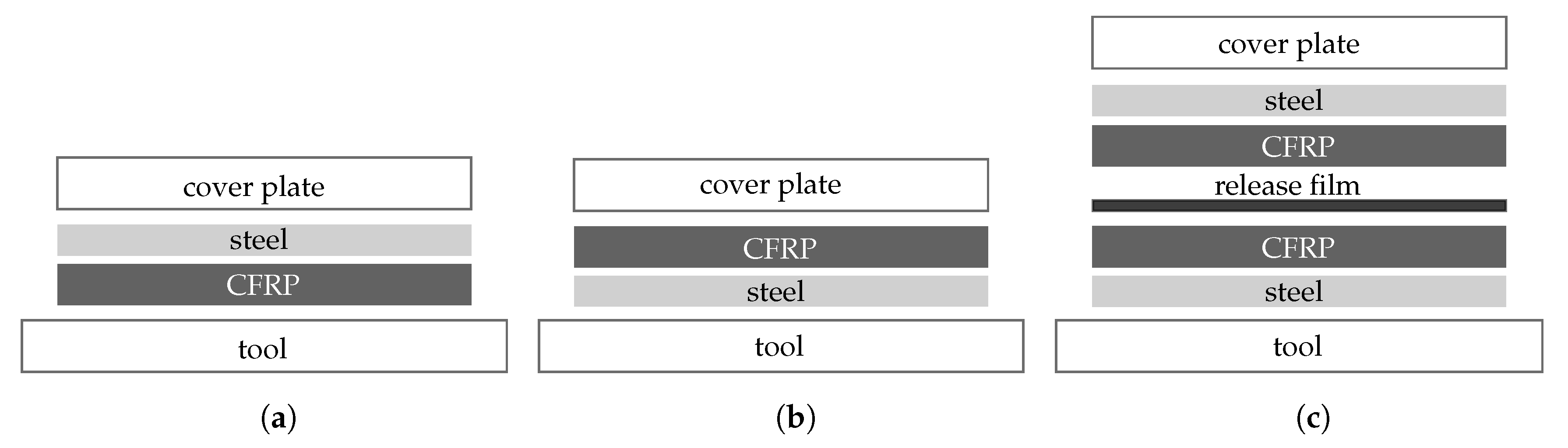
The identifier of the sample is developed so that the parameter variation in the parameter space is evident from the identifier itself. An explanation of the specimen labeling is given in

Table 6. Explanation of the logic that is used to label every specimen manufactured, using the specimen with ID14SR-s as an example.

1	No. of steel plies	-
4	No. of CFRP plies	-
S	Tool material	S: steel/A: aluminum
R	Cure cycle	R: recommended/M: modified
-s	Additional information	-s: stacked manufacturing setup/-e: expired CFRP batch

using the specimen with ID14SR-s as an example. The first two digits indicate the number of steel and CFRP plies within the laminate. The next two digits specify the tool material the specimen was manufactured on and the cure cycle (cf. Figure 2). The last digit indicates the manufacturing setup as discussed in Figure 3, as well as the CFRP batch used.

During the preliminary investigations, an expired batch of CFRP material was used besides a new material batch. Due to a high number of freeze–thaw cycles, the initial degree of cure of the expired material is different from the new material. Consequently, comparisons across both material batches will lead to erroneous conclusions. Therefore, the specimens manufactured with the expired CFRP batch will only be taken into account during the preliminary considerations regarding layup, where the deviation between the different layups is greater than the effect of the CFRP batch and hence, the conclusions drawn are valid. Thereafter, specimens made from the expired CFRP batch will be excluded from the discussion.

Every single specimen is evaluated for its respective curvature and stress-free temperature. As discussed in Section 2.4, there is a correlation between curvature and stress-free temperature. However, since the curvature measurement is easier and more accurate compared to the visual $T_{sf}$-determination, the influence of the different parameters is discussed in Section 3.1 using the curvature only. Nevertheless, the same conclusions can be drawn using the stress-free temperature, which is shown in Section 3.2, where the two parameters are correlated with each other.

3.1. Experimental Curvature Analysis

To keep manufacturing efforts within limits, certain FML layups are selected for subsequent investigations during a preliminary study (Section 3.1.1). Subsequently, the influence of tool material (Section 3.1.2) and process modification (Section 3.1.3) on the specimen curvature is evaluated for the selected layups. In the end, all relevant curvatures are compared, and conclusions regarding the influence of the manufacturing setup are drawn (Section 3.1.4).

3.1.1. Preliminary Considerations Regarding Layup

In the literature, many different layup configurations for asymmetric laminates are selected (cf. Table 1). However, the question arises which type of laminate layup is most appropriate in terms of reproducibility. Therefore, five different layup configurations, as shown in

Table 7. Layup variations investigated in this work and resulting metal volume fractions (MVF) and nominal laminate thicknesses. Layups with ID 14 and ID17 are chosen for the subsequent investigations.

ID	Layup	Metal Volume Fraction (MVF) [%]	Nominal Thickness [mm]
13...	St / 03	24	0.51
14...	St  / 04	19	0.64
15...	St / 05	16	0.77
17...	St / 07	12	1.03
1412...	St / 04 / St / 02	24	1.02

, are investigated. These differ in the number of steel and CFRP plies and their position in the laminate stack. The different layup variations result in specimen thicknesses between around $0.5$ $\mathrm{m}$$\mathrm{m}$ and 1 $\mathrm{m}$$\mathrm{m}$. Furthermore, the metal volume fraction (MVF) varies between 12 and 24.

From Figure 10, it can be seen that with increasing specimen thickness, except for layup ID1412, the radius of the respective specimens increases. Specimens with layup ID13 produced very small radii resulting in difficulties during measurement with the laser scanning technique. Furthermore, the handling of these specimens is more complicated because of their small thickness and hence low stiffness. Therefore, the curvature measurements can be influenced by gravitation, which depends on the placement of the specimen during the measurement. On the other hand, the specimens with ID1412 are not covered by the analytical solution anymore since they do not represent a classic bimetal. Therefore, these two laminates (ID13 and ID1412) are excluded from any further considerations in the context of this work. Likewise, the layup ID15 is excluded to have a greater difference in terms of thickness and MVF between the two remaining layups. Nevertheless, all layups showed comparable standard deviations during curvature measurements. However, it will be shown in a subsequent section that larger radii show better agreement with the analytical and numerical solution.

The layups with ID14 and ID17 are consequently selected for all the subsequent investigations to determine the influence of the different variables during manufacturing on the curvature.

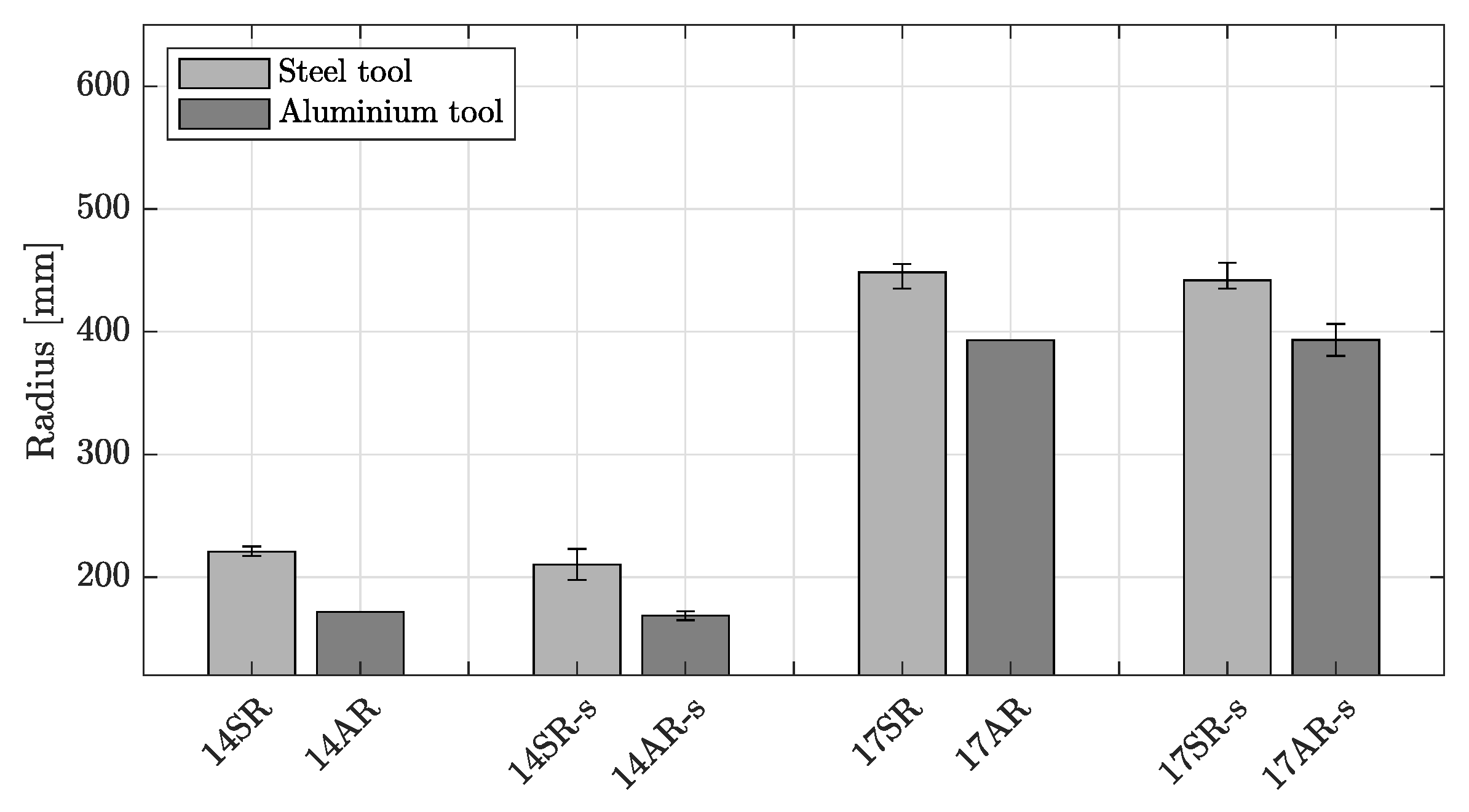
3.1.2. Influence of Tool Material on Specimen Curvature

One great extrinsic contributor to the residual stress level in an FML is the material of the tool [46]. Therefore, two common tool materials in composite manufacturing, steel and aluminum, are chosen to compare their influence on the specimen curvature. The results are shown in Figure 11 for the two selected layups (ID14 and ID17).

It is obvious that specimens manufactured on the aluminum tool show a smaller radius for all investigated configurations compared to the specimens manufactured on the steel tool. This effect can be attributed to the mismatch of the coefficients of thermal expansion between laminate and tool, which results in warpage of the specimen after manufacturing. The steel tool and cover plates show a similar thermal expansion behavior as the steel plies in the laminate themselves (approx. 19 ppm /$\mathrm{K}$, cf. Table 4). The aluminum tool and cover plates, however, possess higher coefficients of thermal expansion of around 24 ppm /$\mathrm{K}$. Hence, using the aluminum tool, the layers close to the tool surface are pre-strained during the heating phase before curing since the aluminum experiences higher thermal expansion. This results in a strain gradient through the thickness of the specimen. These strains are superpositioned with the thermal cure strains resulting from the thermal incompatibility between steel and CFRP layers and are locked into the laminate during resin solidification. After demolding, this results in a different curvature compared to the specimens manufactured on the steel tool. Although the specimens were separated from the tool by using release film, the autoclave pressure and vacuum increase the friction coefficient between the laminate and tool. Since the steel tool and metal layer in the laminate have comparable CTEs, the effect of warpage is not as relevant for the specimens manufactured on the steel tool.

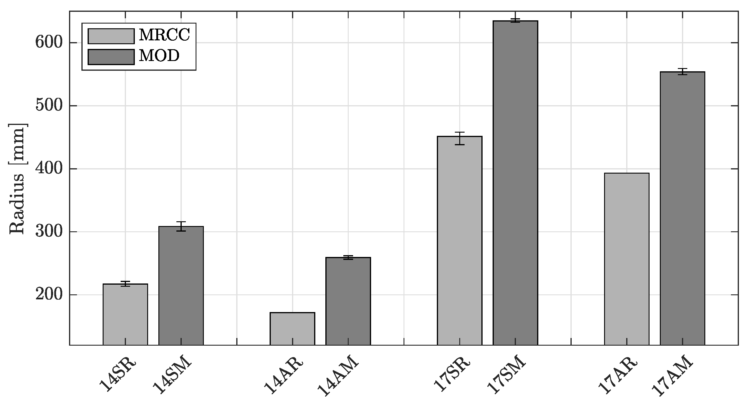
3.1.3. Influence of Cure Cycle on Specimen Curvature

The other important extrinsic parameter affecting the residual stress state in a laminate is the cure cycle and in particular the temperature profile during cure. Therefore, two different cure cycles that were developed for residual stress manipulation are taken from the literature and compared to each other in terms of specimen curvature (cf. Section 2.2.1). To assure a significant comparison, specimens with layup ID14 and ID17 are manufactured during two production runs, while at the same time the two tool materials and three manufacturing setups are used. This is achieved by using two different tools within the same autoclave loading. The resulting curvatures for the specimens manufactured in these two cure cycles are shown in Figure 12.

The plot shows that the two different cure cycles can be clearly distinguished by the radius of the specimens. For all specimens, the MOD cure cycle shows larger radii compared to the MRCC. This behavior is expected since the MOD cycle was developed to reduce residual stresses in a specimen, which consequently results in less curvature and hence larger radii. The MOD cure cycle increases the radius by 42 to 50% for the specimens with ID14 and by around 40% for the specimens with ID17.

3.1.4. Comparison of Curvatures across All Specimens

In Figure 13, the radii of all specimens are plotted for the layups ID14 (Figure 13a) and ID17 (Figure 13b) for general comparison. The two main influencing factors, tool material and cure cycle, clearly distinguish the different curvature levels, which is particularly pronounced in layup ID17.

Furthermore, slight deviations can be recognized within the specimens with identical cure cycle and tool material but different manufacturing setups. The stacked setup, indicated by “-s” in the specimen ID, tendentially shows smaller radii and a larger standard deviation compared to the specimens manufactured on their own between tool and cover plate.

Visual inspection of the specimens manufactured with the stacked setup revealed that the CFRP face of these specimens shows a high surface roughness, whereas the specimens manufactured solely between tool and cover plate possess a surface roughness comparable to the surface of the tool. The high roughness of the stacked specimens can be explained by the lack of a rigid metal tool or cover plate on the CFRP surface. This leads to the fibers interacting with the surface of the opposite specimen since they are only separated by a thin release film. As a result, the surface roughness leads to locally varying laminate thicknesses and hence local differences in bending stiffness and metal volume fractions. These differences increase the variability in the curvature evaluation and complicate the comparability to analytical and numerical derived values. Therefore, the stacked manufacturing setup with CFRP facing CFRP is not recommended by the authors for further investigations.

3.2. Correlation of Curvature and Stress-Free Temperature

Not only the curvature but also the stress-free temperature for all the specimens was determined in a laboratory oven using the method described in Section 2.3.2. In Figure 14, the resulting stress-free temperatures for all specimens of the layups ID14 and ID17 are plotted against their radii. The two different layup configurations can be clearly distinguished by the radius. However, the stress-free temperatures are rather independent of the layup and only sensitive to the extrinsic parameters such as tool material (A: aluminum and S: steel) and cure cycle (R: MRCC and M: MOD). The different extrinsic influences can be differentiated independently of the layup through the horizontal lines in the figure. For the layup with ID14, there is slightly more scattering within the experimental data, which could already be seen in Figure 13a compared to the layup with ID17 (Figure 13b).

Furthermore, the analytical correlation (see Equation (1)) between the radius and stress-free temperature is calculated for the respective layups and added to the figure. The dashed lines represent this solution calculated with the material parameters given in Table 4. The analytics provide a good fit for the experimental data.

From the 3D-optical measurements of every specimen, it is found that the specimen thickness in reality is slightly smaller than the nominal thickness. This can also be observed in Figure 5b, where the mean specimen thickness shows to be approximately 0.625– $0.63$ $\mathrm{m}$$\mathrm{m}$ compared to the nominal thickness of $0.64$ $\mathrm{m}$$\mathrm{m}$ for that specimen. Therefore, the grey area around the analytical solution in Figure 14 shows the uncertainty due to a reduction in specimen thickness by $0.015$ $\mathrm{m}$$\mathrm{m}$ assuming a constant thickness ratio m in Equation (1).

Changing the thickness ratio m has an even larger effect on the analytical solution because the thickness ratio m enters the equation with a higher power. Reducing the steel ply thickness increases the respective stress-free temperature, while a reduction of the CFRP ply thickness reduces the stress-free temperature for a given radius. From Equation (1), it can be seen that the ply thickness is the most sensitive parameter in the analytical solution. However, uncertainties in the other material parameters, i.e., stiffness and coefficient of thermal expansion, can also influence the analytical results.

Table 8. Uncertainties in material parameters and their consequence for the analytical stress-free temperature calculation from the given radius.

FML Constituent	Material Parameter	Variation	Direction of Change in ${\mathit{T}}_{\mathbf{sf}}$
CFRP	t	↑	↑
	E	↑	↑
	$\alpha$	↑	↑
Steel	t	↑	↓
	E	↑	↓
	$\alpha$	↑	↓

shows the direction of the influence on $T_{sf}$ when increasing each parameter for a given radius.

Remembering the stress state from Figure 9, it is clear that the CFRP layers are in a compressive stress state. Therefore, the question arises whether the tensile modulus is the relevant material parameter. Table 8 reveals that reducing the modulus of elasticity to its compressive value given in Table 4, results in reduced stress-free temperatures. This is also shown in Figure 14 for the analytical solution with $E_1^c$ as calculation parameter. The result is lower stress-free temperatures for a given radius. From the figure and the correlation of the data points, however, it cannot be concluded whether the compression modulus $E_1^c$ increases the agreement between experiment and analytic solution.

The numerical results derived from the FEA model, as described in Section 2.5, are congruent to the analytical solutions. In Figure 14, the numerical calculated stress-free temperatures are plotted for the the analytical solution using $E_1^c$ and the relevant discrete radii.

3.3. Transformation into Residual Stresses and Validation Using the Strain Gauge Method

In the previous section, it was shown that the correlation between curvature and stress-free temperature within the experimental data is also found in the analytical and numerical solutions. Furthermore, it could be proven that the stress-free temperature is rather independent of the layup. Therefore, it can be assumed that laminates manufactured within the same process cycle on the same tool possess the same stress-free temperature $T_{sf}$. This $T_{sf}$ can consequently be used to calculate the resulting residual stresses for all the laminates within the same batch using Equation (2).

To validate this, the strain gauge technique described in Section 2.3.3 is used. A specimen with layup ID17 is equipped with a strain gauge on the metal ply (cf. Figure 7) and consequently cured in the autoclave on a steel tool using the MRCC. The resulting curvature and stress-free temperature likewise are plotted into Figure 14. Again, it correlates very well with the analytical solution. However, it deviates slightly from the other specimens manufactured with the same tool and cure cycle. This can potentially be attributed to the different manufacturing runs, the strain gauge bonded to the specimen, and the fact that no trimming was used for this specimen in order to not damage the strain gauge.

The resulting strain measurements over temperature, recorded with the strain gauge throughout the entire manufacturing cycle, are shown in Figure 15a. The progression of the strain curve is consistent with previous strain measurements (cf. [10]). However, at the final cure temperature of 180 ${}^{\circ }\mathrm{C}$, the strain gauge signal was lost but could be recovered after cooling down to room temperature. Therefore, the strains during cool-down result from linear interpolation between the last recorded value at 180 ${}^{\circ }\mathrm{C}$ and the first recorded value at room temperature which is indicated by the dotted line. The strains during cool-down ($t_2\to t_3$) are expected to be rather linear as was shown in [10]. Therefore, no error is assumed to be introduced due to the malfunction of the strain gauge. During demolding of the specimen from the tool surface at room temperature after curing ($t_3\to t_4$), a significant decrease in the residual strain level can be observed. The specimen transitions from its flat state on the tool into the curved state, while releasing some of the inherent residual strains through geometric distortion.

Figure 15b zooms into the demolding step and shows the strains over time. When the specimen is still in its flat state, because the vacuum bag is forcing the specimen onto the flat tool surface, a strain level of 2160 $\mathsf{\mu }$$\mathrm{m}$/$\mathrm{m}$ is measured in the metal ply. After demolding, the asymmetric specimen is allowed to relieve some of the introduced stresses through deformation. Consequently, the measured residual strain in the metal ply rapidly reduces to 696 $\mathsf{\mu }$$\mathrm{m}$/$\mathrm{m}$.

The experimentally determined parameters of the instrumented specimen can now be compared to different calculation strategies.

Table 9. Comparison of measured strains (strain gauge) and calculated strains using measured curvature or measured $T_{sf}$. Values are given for compression and tension moduli of the CFRP material at a reference temperature of $T_r=21{}^{\circ }\mathrm{C}$. The strain delta indicates the difference between measured and calculated strains. Right-hand arrows indicate calculated values with the input parameters to their left.

		Radius	${\mathit{T}}_{\mathbf{sf}}$	Strain Flat	Strain Delta
		(mm)	(°C)	(µm m−1)	(%)
	Experiment	GOM ATOS:	Oven:	Strain gauge:	-
		482	169	2175
$E_1^t$	Strain from exp. $T_{sf}$	-	169	→ 2320	+6.7
$E_1^t$	Strain from exp. radius	482	→176	→ 2429	+11.7
$E_1^c$	Strain from exp. $T_{sf}$	-	169	→ 2270	+4.4
$E_1^c$	Strain from exp. radius	482	→166	→ 2224	+2.3

shows the experimental values for a reference temperature of 21 ${}^{\circ }\mathrm{C}$. The deviations between the values in Figure 15b and Table 9 result from the different temperature levels. While the strain gauge measurements were taken at 19 ${}^{\circ }\mathrm{C}$, the values in the table were interpolated for a room temperature of 21 ${}^{\circ }\mathrm{C}$ since the curvature measurements were taken in a controlled lab environment at a temperature of 21 ${}^{\circ }\mathrm{C}$.

At the bottom of Table 9, the resulting strains are calculated by using the measured stress-free temperature and by using the measured radius of the specimen, respectively. The results show that using the experimentally determined $T_{sf}$, yields slightly higher calculated residual strains (+ 145 $\mathsf{\mu }$$\mathrm{m}$/$\mathrm{m}$). If the measured radius is taken as a starting point and a corresponding stress-free temperature is determined with the aid of the analytical solution, the result is a residual strain that is + 254 $\mathsf{\mu }$$\mathrm{m}$/$\mathrm{m}$ higher than in the SG measurement.

This calculation is less sensitive to a change in thickness of the individual layers, as was the case during the analytical curvature determination. However, using the reduced modulus of elasticity due to the fact that compressive stresses act within the CFRP plies results in strains that are closer to the experimentally determined strain in the flat state. By using $E_1^c$ for the CFRP, the deviations between CLT and experiment can be reduced to values below 5%.

The results of the combined experiment show that both approaches either using the stress-free temperature or the specimens curvature are likewise applicable to determine the residual strains in an FML. With this in mind, the relevant stress-free temperatures can likewise be used to calculate the residual strains or stresses in an arbitrary laminate manufactured with the same process parameters using Equation (2).

4. Discussion

An essential finding of this work is the fact that the stress-free temperature is independent of the layup and only sensitive to extrinsic process parameters. Hence, information derived from asymmetric specimens can be directly used to quantify the residual stress state in laminates with different and more complex layups. Therefore, the use of asymmetric specimens seems to be a suitable method to monitor manufacturing processes and determine residual stress states in FML.

However, the influence of warpage needs to be considered to avoid false assumptions. While warpage mainly affects laminates with thicknesses below 1 $\mathrm{m}$$\mathrm{m}$, thick laminates are not affected [26]. The asymmetric laminates in this work are all in the range of 0.5– 1 $\mathrm{m}$$\mathrm{m}$, and the tool material shows to be a significant contributor to the residual stress state in the specimens. However, for a thicker laminate, this does not necessarily need to hold true. Therefore, it is assumed that by keeping the influence of the tool within the asymmetric specimens to a minimum by using compliant tool CTEs, the accuracy of the proposed method is increased.

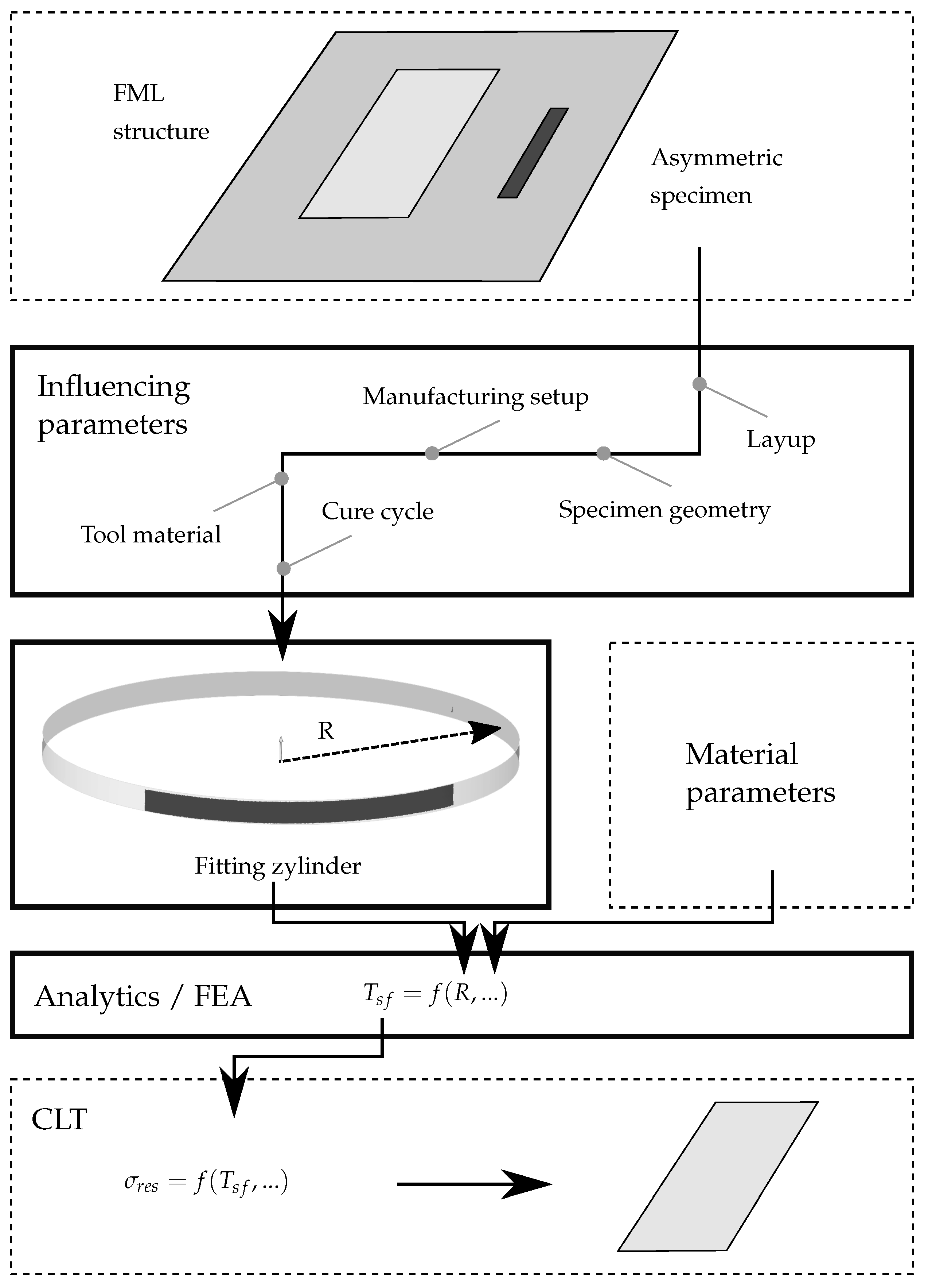
The use of asymmetric samples for process monitoring and in particular for residual stress quantification is shown schematically in the form of a flowchart in Figure 16. The boxes framed with thick lines in the figure indicate the focus of this work.

It was shown that the curvature and stress-free temperature of asymmetric laminates can be accurately determined using experimental methods. However, curvature measurement using a 3-dimensional scanning head seems to be the most accurate method compared to the $T_{sf}$-determination or other curvature measurement techniques and is, therefore, to be preferred. During curvature measurements, it is important to also determine the ambient temperature because it is needed as a reference temperature during subsequent calculations.

Furthermore, the results reveal that a significant correlation between curvature and stress-free temperature exists for asymmetric specimens. However, the laminate layup, the manufacturing setup and the specimen postprocessing need to be considered to reduce the scattering within the experimental data. Thicker laminates that result in larger radii are favorable. Thin laminates and consequently small radii could potentially introduce non-linear effects that increase scattering and can lead to deviations between experiment and analytical solution. Furthermore, the manufacturing setup where two specimens are placed on top of each other with their CFRP sides is to be avoided. It is assumed that a setup where the steel sides face each other shows comparable results to the single setups. However, this placement strategy was not investigated in this work. A trimming operation after curing of the specimens is recommended to reduce the influence of edge effects on the evaluated parameter. It is assumed that trimming reduces the scattering within the experimental results. However, the difference was not quantified within this work. It is recommended to use water-jet cutting instead of a saw to reduce any thermal influences on the specimen state.

Analytical and numerical methods are likewise able to depict the correlation between curvature and $T_{sf}$. However, it was shown that both solutions are very sensitive to uncertainties in the specimen thickness and material parameters. Therefore, a comprehensive set of material parameters is necessary for accurate calculations. To have more accurate thickness information, an analysis of a cross-sectional cut could be integrated into the process. Moreover, in this work, only the modulus of elasticity of the steel material was experimentally determined. All other material parameters were taken from the literature. To improve the results in future research, the other relevant material parameters should also be verified by experiments.

The parameters derived from the asymmetric specimen are in accordance with in situ strain gauge measurements. Depending on the material parameters used, deviations below 5 and 12 could be achieved. In the next step, this validation needs to be verified for a larger specimen set and different parameter variations as well as for a more complex FML structure. This is indicated by the top and bottom boxes in Figure 16. In addition to the classical laminate theory, this step can also be coupled with an FEA model such that the stress-free temperature is used as an input parameter within this model. This way, more complex stress states due to complex layups and geometries could be described.

5. Conclusions

In this work, it was shown that the accuracy of the curvature analysis of asymmetric specimens to determine the residual stress state in an FML depends highly on appropriate laminate layups, evaluation techniques and comprehensive material parameters.

It was found that thin laminates show non-linear effects and are further prone to additional influences due to warpage. Therefore, thicker asymmetric laminates that result in larger radii are to be preferred in combination with CTE-compliant tools. Furthermore, by using a small width-to-length aspect ratio, effects due to transverse curvatures can be neglected. Water jet cutting was identified as the best solution for trimming the asymmetric fiber metal laminates after manufacturing.

Specimens manufactured under consideration of these findings show a good correlation between their experimentally determined curvature and stress-free temperature. Beyond that, this correlation is in good agreement with analytical and numerical solutions. For the experimental parameter evaluation, the curvature measurement using optical 3D-scanning techniques seems to be the favored option, since the stress-free temperature measurement in an oven comes with limited accuracy due to the experimental setup.

The fact that a good correlation between stress-free temperature and curvature exists for the asymmetric laminates, which is further backed by analytical calculations, makes it possible to transfer the information gained from asymmetric specimens to more complex FML structures manufactured within the same process. Furthermore, asymmetric specimens are suitable for process monitoring since they are sensitive to changing process conditions as was shown by using a temperature-modified cure cycle.

Hence, the stress-free temperature gained from such asymmetric laminates can consequently be used for the residual stress quantification in more complex FML structures manufactured within the same process. The proposed workflow in Figure 16 highlights the steps to be followed when asymmetric laminates are added during manufacturing for process monitoring. Future work needs to concentrate mainly on the validation of the transfer of residual stress levels from asymmetric specimens to a complex structure.

The findings in this work are not only valid for FMLs, but it is assumed that they can also be adapted to other laminated composite materials. However, due to the high anisotropy of the FML, the effects considered are more prominent in an FML consisting of CFRP and steel.

References

1. Alderliesten, R. Fatigue and Fracture of Fibre Metal Laminates; Springer: Cham, Switzerland, 2017; Volume 236. [Google Scholar]
2. Vlot, A.; Gunnink, J.W. Fibre Metal Laminates: An Introduction; Springer: Dordrecht, The Netherlands, 2001. [Google Scholar]
3. Petersen, E.; Stefaniak, D.; Hühne, C. Experimental investigation of load carrying mechanisms and failure phenomena in the transition zone of locally metal reinforced joining areas. Compos. Struct. 2017, 182, 79–90. [Google Scholar] [CrossRef]
4. Boose, Y.; Kappel, E.; Stefaniak, D.; Prussak, R.; Pototzky, A.; Weiß, L. Phenomenological investigation on crash characteristics of thin layered CFRP-steel laminates. Int. J. Crashworthiness 2020, 182, 1–10. [Google Scholar] [CrossRef]
5. Düring, D.; Petersen, E.; Stefaniak, D.; Hühne, C. Damage resistance and low-velocity impact behaviour of hybrid composite laminates with multiple thin steel and elastomer layers. Compos. Struct. 2020, 238, 111851. [Google Scholar] [CrossRef]
6. Zobeiry, N.; Poursartip, A. The origins of residual stress and its evaluation in composite materials. In Structural Integrity and Durability of Advanced Composites; Beaumont, P.W.R., Ed.; Woodhead Publishing Series in Composites Science and Engineering; Elsevier: Amsterdam, The Netherlands, 2015; pp. 43–72. [Google Scholar] [CrossRef]
7. Johnston, A.A. An Integrated Model of the Development of Process-induced Deformation in Autoclave Processing of Composite Structures. Ph.D. Thesis, University of British Columbia, Vancouver, BC, Canada, 1997. [Google Scholar] [CrossRef]
8. Abouhamzeh, M. Distortions and Residual Stresses of GLARE Induced by Manufacturing. Ph.D. Thesis, Delft University of Technology, Delft, The Netherlands, 2016. [Google Scholar] [CrossRef]
9. Kappel, E.; Prussak, R.; Wiedemann, J. On a simultaneous use of fiber-Bragg-gratings and strain-gauges to determine the stress-free temperature Tsf during GLARE manufacturing. Compos. Struct. 2019, 227, 111279. [Google Scholar] [CrossRef]
10. Wiedemann, J.; Prussak, R.; Kappel, E.; Hühne, C. In-situ quantification of manufacturing-induced strains in fiber metal laminates with strain gauges. Compos. Struct. 2022, 691, 115967. [Google Scholar] [CrossRef]
11. Luyckx, G.; Voet, E.; Lammens, N.; Degrieck, J. Strain measurements of composite laminates with embedded fibre bragg gratings: Criticism and opportunities for research. Sensors 2011, 11, 384–408. [Google Scholar] [CrossRef] [Green Version]
12. Tsukada, T.; Takeda, S.; Minakuchi, S.; Iwahori, Y.; Takeda, N. Evaluation of the influence of cooling rate on residual strain development in unidirectional carbon fibre/polyphenylenesulfide laminates using embedded fibre Bragg grating sensors. J. Compos. Mater. 2017, 51, 1849–1859. [Google Scholar] [CrossRef]
13. Prussak, R.; Stefaniak, D.; Hühne, C.; Sinapius, M. Evaluation of residual stress development in FRP-metal hybrids using fiber Bragg grating sensors. Prod. Eng. 2018, 12, 259–267. [Google Scholar] [CrossRef]
14. Twigg, G.; Poursartip, A.; Fernlund, G. An experimental method for quantifying tool–part shear interaction during composites processing. Compos. Sci. Technol. 2003, 63, 1985–2002. [Google Scholar] [CrossRef]
15. Crasto, A.S.; Kim, R.Y. On the Determination of Residual Stresses in Fiber-Reinforced Thermoset Composites. J. Reinf. Plast. Compos. 1993, 12, 545–558. [Google Scholar] [CrossRef]
16. Unger, W.J.; Hansen, J.S. The Effect of Cooling Rate and Annealing on Residual Stress Development in Graphite Fibre Reinforced PEEK Laminates. J. Compos. Mater. 1993, 27, 108–137. [Google Scholar] [CrossRef]
17. Cowley, K.D.; Beaumont, P.W. The measurement and prediction of residual stresses in carbon-fibre/polymer composites. Compos. Sci. Technol. 1997, 57, 1445–1455. [Google Scholar] [CrossRef]
18. Prussak, R.; Stefaniak, D.; Hühne, C.; Sinapius, M. Residual Stresses in Intrinsic UD-CFRP-Steel-Laminates-Experimental Determination, Identification of Sources, Effects and Modification Approaches. Mater. Sci. Forum 2015, 852–826, 369–376. [Google Scholar] [CrossRef]
19. Jeronimidis, G.; Parkyn, A.T. Residual Stresses in Carbon Fibre-Thermoplastic Matrix Laminates. J. Compos. Mater. 1988, 22, 401–415. [Google Scholar] [CrossRef]
20. Schulte, K.J.; Hahn, H.T. Prediction and Control of Processing-Induced Residual Stresses in Composites. Part 2: AS4/PEEK Composite, Final Technical Report; Composites Manufacturing Technology Center, Pennsylvania State University: University Park, PA, USA, 1989. [Google Scholar]
21. O’Brien, T.K. Fatigue Delamination Behavior of PEEK Thermoplastic Composite Laminates. J. Reinf. Plast. Compos. 1988, 7, 341–359. [Google Scholar] [CrossRef]
22. Pagano, N.J.; Hahn, H.T. Evaluation of Composite Curing Stresses. In Mechanics of Composite Materials; Gladwell, G.M.L., Reddy, J.N., Eds.; Springer: Dordrecht, The Netherlands, 1994; Volume 34, pp. 57–69. [Google Scholar]
23. Prussak, R.; Stefaniak, D.; Kappel, E.; Hühne, C.; Sinapius, M. Smart cure cycles for fiber metal laminates using embedded fiber Bragg grating sensors. Compos. Struct. 2019, 213, 252–260. [Google Scholar] [CrossRef]
24. Schürmann, H. Konstruieren mit Faser-Kunststoff-Verbunden; Springer: Berlin/Heidelberg, Germany, 2007. [Google Scholar] [CrossRef]
25. Both, J.C. Tragfähigkeit von CFK-Metall-Laminaten unter Mechanischer und Thermischer Belastung. Ph.D. Thesis, Technische Universität München, München, Germany, 2014. [Google Scholar]
26. Albert, C.; Fernlund, G. Spring-in and warpage of angled composite laminates. Compos. Sci. Technol. 2002, 62, 1895–1912. [Google Scholar] [CrossRef]
27. Kappel, E.; Stefaniak, D.; Fernlund, G. Predicting process-induced distortions in composite manufacturing—A pheno-numerical simulation strategy. Compos. Struct. 2015, 120, 98–106. [Google Scholar] [CrossRef]
28. Potter, K.D.; Campbell, M.; Langer, C.; Wisnom, M.R. The generation of geometrical deformations due to tool/part interaction in the manufacture of composite components. Compos. Part A Appl. Sci. Manuf. 2005, 36, 301–308. [Google Scholar] [CrossRef]
29. Stefaniak, D.; Kappel, E.; Spröwitz, T.; Hühne, C. Experimental identification of process parameters inducing warpage of autoclave-processed CFRP parts. Compos. Part A Appl. Sci. Manuf. 2012, 43, 1081–1091. [Google Scholar] [CrossRef]
30. White, S.R.; Hahn, H.T. Cure Cycle Optimization for the Reduction of Processing-Induced Residual Stresses in Composite Materials. J. Compos. Mater. 1993, 27, 1352–1378. [Google Scholar] [CrossRef]
31. Kim, H.S.; Park, S.W.; Lee, D.G. Smart cure cycle with cooling and reheating for co-cure bonded steel/carbon epoxy composite hybrid structures for reducing thermal residual stress. Compos. Part A Appl. Sci. Manuf. 2006, 37, 1708–1721. [Google Scholar] [CrossRef]
32. Kim, Y.K.; Daniel, I.M. Cure Cycle Effect on Composite Structures Manufactured by Resin Transfer Molding. J. Compos. Mater. 2002, 36, 1725–1743. [Google Scholar] [CrossRef]
33. Kim, S.S.; Murayama, H.; Kageyama, K.; Uzawa, K.; Kanai, M. Study on the curing process for carbon/epoxy composites to reduce thermal residual stress. Compos. Part A Appl. Sci. Manuf. 2012, 43, 1197–1202. [Google Scholar] [CrossRef]
34. DIN EN ISO 6892-1:2020-06; Metallische Werkstoffe–Zugversuch, Teil 1: Prüfverfahren bei Raumtemperatur. Beuth-Verlag: Berlin, Germany, 2020. [CrossRef]
35. National Institute for Aviation Research. Hexcel 8552 AS4 Unidirectional Prepreg at 190 gsm & 35% RC Qualification Material Property Data Report; Wichita State University: Wichita, KS, USA, 2011. [Google Scholar]
36. Hexcel Corporation. Product Data Sheet HexPly 8552; Hexcel Corporation: Stamford, CT, USA, 2020. [Google Scholar]
37. Kappel, E. On thermal-expansion properties of more-orthotropic prepreg laminates with and without interleaf layers. Compos. Part C Open Access 2020, 3, 100059. [Google Scholar] [CrossRef]
38. Stefaniak, D.; Kappel, E.; Kolesnikov, B.; Hühne, C. Improving the mechanical performance of unidirectional CFRP by metal-hybridization. In Proceedings of the ECCM15-15th European Conference on Composite Materials, Venice, Italy, 24–28 June 2012. [Google Scholar]
39. Blohowiak, K.Y.; Osborne, J.H.; Krienke, K.A. Surface Pretreatment of Metals to Activate the Surface for Sol-Gel Coating. U.S. Patent No. 5,869,140, 9 February 1999. [Google Scholar]
40. Stefaniak, D. Improving Residual Strength of Unidirectionally Reinforced Plastic Laminates by Metal Layering. Ph.D. Thesis, Technische Universität Carola-Wilhelmina zu Braunschweig, Braunschweig, Germany, 2017. [Google Scholar]
41. 3M Aerospace and Commercial Transportation Division. 3M™ Surface Pre-Treatment AC-130-2; 3M Aerospace and Commercial Transportation Division: Minneapolis, MN, USA, 2015. [Google Scholar]
42. Khatkhate, A.M.; Singh, M.P.; Mirchandani, P.T. A Parametric Approximation for the Radius of Curvature of a Bimetallic Strip. Int. J. Eng. Res. 2017, V6, 647–650. [Google Scholar] [CrossRef]
43. Angel, G.D.; Haritos, G.K. An Immediate Formula for the Radius of Curvature of A Bimetallic Strip. Int. J. Eng. Res. Technol. 2013, 2, 1312–1319. [Google Scholar]
44. Timoshenko, S. Analysis of Bi-Metal Thermostats. J. Opt. Soc. Am. 1925, 11, 233. [Google Scholar] [CrossRef]
45. Nettles, A.T. Basic Mechanics of Laminated Composite Plates; Technical Report: NASA-RP-1351; National Aeronautics and Space Administration, Marshall Space Flight Center: Huntsville, AL, USA, 1994. [Google Scholar]
46. Wisnom, M.R.; Gigliotti, M.; Ersoy, N.; Campbell, M.; Potter, K.D. Mechanisms generating residual stresses and distortion during manufacture of polymer–matrix composite structures. Compos. Part A Appl. Sci. Manuf. 2006, 37, 522–529. [Google Scholar] [CrossRef]
Figure 1. Stress over strain resulting from tensile tests to determine the Young’s modulus of cold rolled 1.4310 stainless steel. (a) Stress–strain curve in direction of rolling (DOR); (b) Stress–strain curve transverse to DOR.
Jcs 06 00329 g001
Figure 2. Two different temperature profiles during autoclave cure for the two considered manufacturing processes MRCC and MOD.
Jcs 06 00329 g002
Figure 3. Different manufacturing setups regarding the placement of the layer stack between tool and cover plate. (a) Single setup: CFRP on tool; (b) Single setup: steel on tool; (c) Stacked setup.
Jcs 06 00329 g003
Figure 4. Dimensions of the manufactured and trimmed specimens in their plane state.
Jcs 06 00329 g004
Figure 5. Measurement techniques for the curvature evaluation of asymmetric specimens: (a) laser distance sensor for specimen height evaluation; (b) 3D point cloud representation of a specimen with GOM ATOS (legend indicates the laminate thickness).
Jcs 06 00329 g005
Figure 6. Stress-free temperature measurement through reheating of a specimen after manufacturing in a lab oven and determination of the temperature when the specimen reaches its flat state. (a) Curved specimen at room temperature; (b) Flat specimen at stress-free temperature.
Jcs 06 00329 g006
Figure 7. Manufacturing setup for specimen equipped with strain gauge.
Jcs 06 00329 g007
Figure 8. FEA model to determine the stress-free temperature for a given curvature of an asymmetric specimen. (a) Curved specimen in its initial state; (b) Flat specimen after applied temperature change.
Jcs 06 00329 g008
Figure 9. Residual stress state through the thickness in a generic FML after manufacturing at elevated temperature and cool down to room temperature.
Jcs 06 00329 g009
Figure 10. Variations in the layup and consequent specimen thicknesses result in significantly different radii of the asymmetric specimen.
Jcs 06 00329 g010
Figure 11. Specimens manufactured on the aluminum tool show significantly smaller radii compared to the specimen manufactured on the steel tool.
Jcs 06 00329 g011
Figure 12. The modified cure cycle (MOD) clearly increases the radius of asymmetric specimens compared to the manufacturer-recommended cure cycle (MRCC), independent of tool material and specimen layup.
Jcs 06 00329 g012
Figure 13. Difference in specimen radius due to variations in the cure cycle, tool material and manufacturing setup. (a) Specimens with layup ID14; (b) Specimens with layup ID17.
Jcs 06 00329 g013
Figure 14. Correlation of stress-free temperature with specimen radius and comparison to analytical and numerical derived values. Specimens are clustered according to their stress-free temperature and the two extrinsic influencing factors: tool material and cure cycle.
Jcs 06 00329 g014
Figure 15. Strain gauge recordings during manufacturing and demolding of the instrumented asymmetric specimen. Strain readings start at t 1 and finish at t 4 . (a) Strains over temperature during cure; (b) Strains over time during demolding.
Jcs 06 00329 g015
Figure 16. Proposed workflow to use asymmetric specimens for residual stress quantification of FML structures. The focus of this paper is indicated by the boxes framed with thick lines.
Jcs 06 00329 g016