Abstract
In this work, a supervised machine learning (ML) model was developed to detect flow disturbances caused by the presence of a dissimilar material region in liquid moulding manufacturing of composites. The machine learning model was designed to predict the position, size and relative permeability of an embedded rectangular dissimilar material region through use of only the signals corresponding to an array of pressure sensors evenly distributed on the mould surface. The burden of experimental tests required to train in an efficient manner such predictive models is so high that favours its substitution with synthetically-generated simulation datasets. A regression model based on the use of convolutional neural networks (CNN) was developed and trained with data generated from mould-filling simulations carried out through use of OpenFoam as numerical solver. The evolution of the pressure sensors through the filling time was stored and used as grey-level images containing information regarding the pressure, the sensor location within the mould and filling time. The trained CNN model was able to recognise the presence of a dissimilar material region from the data used as inputs, meeting accuracy expectation in terms of detection. The purpose of this work was to establish a general framework for fully-synthetic-trained machine learning models to address the occurrence of manufacturing disturbances without placing emphasis on its performance, robustness and optimization. Accuracy and model robustness were also addressed in the paper. The effect of noise signals, pressure sensor network size, presence of different shape dissimilar regions, among others, were analysed in detail. The ability of ML models to examine and overcome complex physical and engineering problems such as defects produced during manufacturing of materials and parts is particularly innovative and highly aligned with Industry 4.0 concepts.
1. Introduction
Fibre reinforced polymer composites (PMCs) are nowadays widely used in applications that require lightweight materials such as those found in aerospace, automotive, energy, health-care and sports, among others. Structural PMCs are processed by the infiltration of a polymer matrix in the form of a thermoset or thermoplastic resin into a fabric preform, producing materials with optimal stiffness, strength, fatigue performance and resistance to environmental effects [1,2]. The high level of maturity reached as regards design and manufacture of advanced structural composites has enabled their extensive use in civil and military aircraft applications. For instance, the A350XWB contains as much as 53% of the structural weight of components, including carbon fuselage, wings or tail planes [3]. The automation of process steps, the increase of part integration level as well as the continuous demands towards zero-defect manufacturing, guided by Industry 4.0 concepts are the subsequent major steps that will undoubtedly allow future material optimization and cost reduction.
Liquid moulding of composites (LCM) starts with a dry fabric preform which is draped and placed into a mould for its impregnation with a liquid resin by prescribing a pressure gradient [4,5]. After the part is totally impregnated, the resin is cured, normally by the simultaneous action of heat sources until the part becomes solid and can be demoulded. Nowadays, LCM techniques can deliver to the industry high-quality and complex-shape composite articles, providing a solid out-of-autoclave alternative.
Resin transfer moulding (RTM) makes use of a closed solid mould in which the fabric is impregnated by a pressure gradient imposed between the inlet and outlet gates of the mould. Variations of such technologies include, among others, the replacement of a half part of the mold by a vacuum bag in vacuum infusion (VI), the use of auxiliary flow media to induce through-the-thickness flow of resin into the preform (Seemann composite resin infusion molding process, SCRIMP), or the use of flexible membranes as in light RTM (LRTM).
One of the major drawbacks in LCM arises from the inherent uncertainty as regards the flow patterns produced during resin impregnation which are strongly affected by different processing disturbances. For instance, variations of local permeability of the fabric preform triggered by uneven mould clamping, fabric shearing generated during draping operations or unexpected resin channels created at mould edges, also known as race-tracking, result in non-homogeneous resin flow far from theoretical predictions and consequently the formation of dry spots and porous areas. Counteracting against processing disturbances requires its early detection through use of the appropriate sensor networks as well as the implementation of the necessary corrective actions if the quality of the composite article is intended to be secured [6]. This later objective is precisely one of the differential concepts that emanates from Industry 4.0 smart factories which relies on the development of the appropriate cyber-physical systems able to perform automatically diagnosis and detect possible processing faults, as well as implement the necessary corrective actions.
Significant efforts have been made by the scientific and technical community in the last years to spread predictive models based on artificial intelligence (AI) and machine learning concepts (ML) to different sectors. Good examples can be found, for instance, in automated image recognition and computer vision algorithms used in autonomous car driving, fast text language translation and facial recognition, among others [7,8,9]. Such algorithms, when appropriately trained for each individual case, open revolutionary opportunities for other less explored fields such as continuum [10] and fluid mechanics or manufacturing. At this time, it is worth mentioning some interesting contributions close to the topic presented in this paper [11,12,13]. Wu et al. [11] developed a permeability surrogate model based on microstructural images through use of a convolutional neural network (CNN). A training set is generated first by these authors that contains synthetic images of porous microstructures while the corresponding effective permeability is computed, solving numerically the boundary value problem with Lattice Boltzmann methods. The CNN is then trained to learn and link the specific features of the microstructure (e.g., porosity) with the effective permeability value. Overall, surrogate models are viewed as very effective methods to overcome complex problems involving strong non-linearity, uncertainties, accelerating computation times in flow propagation through random media [14].
Although machine learning methods have been extensively used for surrogate modelling, the ability of these technologies to link input and output datasets without taking in consideration the underlying physics made them convenient tools for inverse modelling [12,13]. In this case, a forward model, the physical model, enables the generation of a synthetic output dataset based on the resolution of the governing equations (e.g., a fluids or mechanics problem) given the input dataset. Once the output dataset is generated, it is possible to relate the outputs with their corresponding inputs through use of regression machine learning tools. From an engineering viewpoint, such approximations are of major importance in practical problems such as tomographic reconstruction, computer imaging or sensors. Iglesias et al. [12] used concepts based on Bayesian inference to address the problem of uncertainties of fabric permeability in resin transfer moulding by using information coming from pressure sensors. Lähivaara et al. [13] developed a solution for the determination of the material porosity based on ultrasound tomography through use of CNN. A forward model is used to generate the theoretical response of the ultrasound sensors to a given material with known porosity parameters. The inverse problem is approximated with a regression based CNN which enables the determination of the effective porosity of a material from the direct inspection of the ultrasound transducers response.
The main purpose of this work was to provide a first exploration of machine learning methods to detect automatically flow disturbances caused by the presence of dissimilar permeability regions in liquid moulding of composites. The detection capabilities of the model fall on the analysis of pressure changes recorded by a distributed network of sensors. The model was developed to address the problem of rectangular dissimilar region in a squared flat RTM mould and has been kept intentionally simple with the purpose to explore its learning capabilities. The general description of the methodology is presented in Section 2 including the forward model based on the resolution of the flow propagation problem in porous media. The systematic generation of a fully-based simulation results set corresponding to the physical problem is presented in Section 3 while the general architecture of the neural network model, its training and deploying is described in Section 4. A general discussion on the applicability of the model presented is done in Section 5, while some remarks and conclusions are lastly drawn in Section 6.
2. Model Description
The general description of the model is sketched in Figure 1. An square flat RTM mould containing a dissimilar material region of relative permeability is analyzed, where K and stand for the permeability of the fabric and the dissimilar region embedded, respectively. The position and size of this dissimilar region are defined by and . The forward model uses the 5-tuple input to determine the virtual response of a set of pressure sensors distributed over the mould surface.
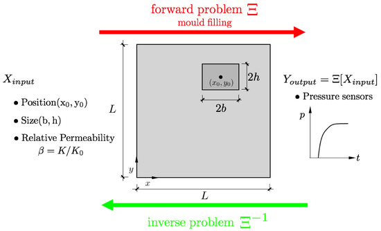
Figure 1.
General description of the problem. Square RTM mould containing a rectangular dissimilar material region with relative permeability of , size and centered at . and K stand for the permeability of the dissimilar region and the surrounding media, respectively.
The Latin Hypercube sampling was used to generate the different realizations of the inputs and the corresponding output dataset is generated, containing all the pressure sensor signals for different dissimilar material cases (). A supervised regression machine learning model based on convolutional neural network is used to approximate the solution of the inverse problem (), thus enabling the position and size of the dissimilar material region to be estimated when the pressure sensor signal information is available. Such a kind of inverse approximation permits the on-line detection of flow disturbances and possible dry spot regions during the resin injection without accessing visually the interior of the mould and by using only the information of the pressure sensors readings.
3. Dataset Synthetic Generation
3.1. Mould Filling Model
The model used in this work is based on the resolution of the Darcy equation for the fluid flow through porous medium. The Darcy equation establishes a linear relation between the average fluid velocity through the fiber preform and the pressure gradient , with the proportionality factor being related to the fabric permeability tensor and the fluid viscosity as
In this equation, x and t stand for the position of a given point in the fabric and the time, respectively. Assuming flow continuity, , the governing equation for the pressure field can be obtained as
Initial () and boundary conditions should be given to determine the evolution of the pressure and velocity fields during the time. Such a problem is normally defined as a moving boundary problem because the flow front position evolves during the time until the preform is completely filled. Normally, if the position of the flow front is known for given time t, the pressure and velocity fields are determined by standard finite element modelling. Once such information is acquired, updating the flow front position for time can be obtained. Several numerical techniques were developed in the past to solve such problems in liquid moulding manufacturing of composites. For instance, the finite element/control volume method uses regions associated with every node to update information about the filling factors through use of the flow rates obtained with the velocity fields. Such numerical methods are implemented in well-known simulation tools such as LIMS from Advani and co-authors [15,16] or PAM-RTM from ESI group. Other ways to simulate mould filling processes are based on the direct solving of the two-phase flow problem by using the Navier-Stokes equations for incompressible fluids. In this case, the continuity equation is accompanied by the linear momentum equation reading as
where S is known as the Darcy–Forchheimer sink term
where D and F stand for material parameters. The second term in Equation (4) is related to inertial effects which are negligible for the case of liquid moulding of composites under low Reynolds number flow. In this situation, the inertial terms related to the velocity can be neglected, recovering the standard Darcy equation with the factor D being the inverse permeability of the fabric. In two-phase flow, the interface between the two fluids, namely resin and air in liquid moulding, is tracked by means of the volume of fluid (VOF) approach by using as a phase variable. This variable ranges between and for the resin and air fluids, respectively. Within this approach, the variable is continuously updated during simulation time by using the advection equation given by
OpenFoam® (Open source Field Operation And Manipulation) [17] is a free open source Computational Fluid Dynamics (CFD) software that can be used to solve the problems related with filling in liquid moulding of composites. OpenFoam includes interFoam a solver for two-phase incompressible, isothermal and immiscible fluids tracking interfaces with the VOF method. Details and performance of the algorithms used to track interfaces as well as pressure and velocity solvers for two-phase flow can be found in [18].
3.2. Mould Filling Simulations Containing Dissimilar Material Regions
The bi-dimensional problem of a square mould of dimensions containing a rectangular region with different permeability is modeled in this section as shown in Figure 2a. This geometrical definition constitutes the base of the mould filling forward problem to be solved by computational fluid mechanics. For simplicity, macroscopic unidirectional flow is induced by the application of a constant pressure condition at while is set in the opposite edge at . Slip-free conditions are applied in the remaining faces of the mould.
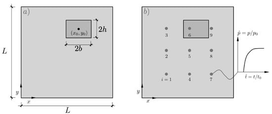
Figure 2.
(a) Definition of the model containing a dissimilar rectangular region with center coordinates , size and permeability , (b) network of pressure sensors equally distributed on the mould surface.
A rectangular region with centre () and size () with dissimilar permeability is inserted in the model, where stands for the permeability of the surrounding material. For simplicity, both permeabilities, and K, were assumed to be isotropic and representative of angle-ply 2D woven preforms although simulations can be carried out by assuming anisotropic behavior without any loss of generality.
Accordingly, the set of non-dimensional numbers and corresponds to the position, size and relative permeability of the dissimilar region defined as a 5-tuple object. A uniform brick cell discretization of the domain was used with in-plane dimensions and with a single cell in the mould through-the-thickness direction. Thus, the models contain 10,000 brick cells which were judged fine enough to capture accurately the flow front position evolution during time. The two fluids selected for the interFoam solver corresponded to water and air, for simplicity. Their density and kinematic viscosity were set to 1000 Kg/m and /s for the water, and 1 Kg/m and /s for the air, respectively. Despite the simplicity of the model presented in this work, more complicated problems including different mould shapes, inlet and outlet configurations among others can be addressed and used for synthetic training of the artificial intelligence method.
To fully explore the problem space, the involved variables were presented in non-dimensional form as , and where and the injection pressure, respectively. This latter value of corresponds exactly to the mould filling time for a perfectly homogeneous distribution of the permeability (). A network of pressure probes equally distributed in the surface of the mould is used to record the time evolution of the fluid pressure (Figure 2b).
Figure 3 shows the position of the front flow for different times obtained for a case with and . The relative permeability in this case was set to . In the early stages, the flow progresses uniformly until it reaches the position of the first dissimilar material region. As the permeability inside the dissimilar region is lower than the surrounding media (), the flow delays with respect to it. Lastly, the flow progresses until the outlet gate but first in the upper part of the mould far from the dissimilar material region. Such a non-uniform flow presented in Figure 3 is reflected in the probe pressure evolution as shown in Figure 4a.
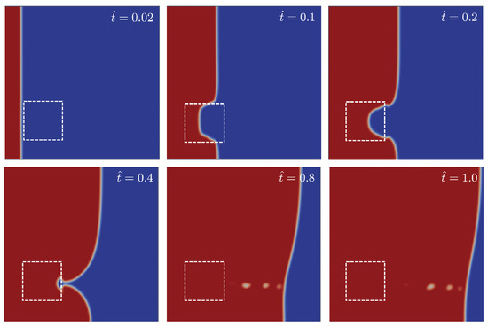
Figure 3.
Snapshots of the flow progress through the mould for different non-dimensional times = 0.02, 0.1, 0.2, 0.4, 0.8 and 1.0. The mould contains a square region of size centered at and with relative permeability of . Flow progress from left to right. Red and blue colours correspond to phase values of and , respectively. For the sake of clarity, white dashed lines corresponding to the dissimilar material region were superimposed.
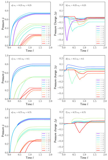
Figure 4.
Non-dimensional pressure evolution for the nine sensors distributed in the mould containing a square dissimilar material region at (a) , (c) and (e) . Dashed lines corresponds with the pressure sensor evolution in the absence of dissimilar material region. The pressure changes in (b,d,f) are as the difference, or perturbation, between the local pressure value with and without dissimilar material region. For visualization purposes, the non-dimensional time was arbitrarily extended to .
The evolution of the nine pressure sensors evenly distributed over the surface of the mould is presented in Figure 4, again expressed as non-dimensional numbers and . Results for three different cases were presented in this figure and correspond to a square region of size located at three positions (a) , (b) and (c) . The shape of the pressure sensor evolution curve was similar in all of them. A sudden increase is produced when the fluid reaches the sensor position and progressively stabilizes to a steady-state value consistent with the pressure gradient induced between the inlet and outlet gates. The dashed lines in Figure 4 were obtained by assuming no dissimilar material region by setting .
The pressure perturbation is also presented in the same figure, defined as the difference between the local pressure obtained in the problem containing the dissimilar region and the problem without dissimilar region. The pressure evolution and/or the perturbations caused by the presence of the dissimilar region could help to ascertain the position, size and intensity of the defect. However, given that its complexity with respect to the random position and size make the problem intractable in terms of mathematical complexity, data science or statistical techniques could be more appropriate for such kind of inverse problems.
The position of the sensor with respect to the location of the dissimilar material region influences the evolution of the pressure. If the sensor is placed upstream from the dissimilar material region, an increase in the pressure is produced as compared with the case without the defect. This effect can be observed in sensors 1, 2 and 3 in Figure 4c,e. However, if the sensor is placed downstream from position of the dissimilar material region, the pressure is delayed to some extent as shown in sensors 1, 2 and 3 in Figure 4a. Both effects are reflected in the pressure perturbation in Figure 4b,d,f, exhibiting a positive change if the sensor is placed upstream and negative in the opposite case. The information of the pressure , or the pressure perturbation , recorded by the sensors was stored as a footprint image and is presented in Figure 5a,b for the three cases presented previously by using a pressure sensor network of .
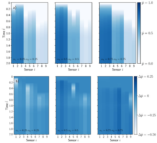
Figure 5.
(a) Sensor footprints corresponding to the plot cases presented in Figure 4. The vertical and horizontal axis of the images corresponded with the non-dimensional time and sensor position . The color intensity reflects the sensor non-dimensional pressure , (b) Pressure perturbation evolution footprint. For visualization purposes, the non-dimensional time was arbitrarily extended to .
3.3. Dataset Generation
Once the forward problem is defined, the complete dataset should be generated. A uniform covering of the whole variable space of the model, namely and , results in intractable problem size. For simplicity, the variables were assumed to follow uniform random probability distributions as , , . and distributions ensure that the dissimilar material region is entire contained in the mould surface. Assuming, for instance, ten different random realizations of the aforementioned variables, the number of combinations is which seems unfeasible from a practical viewpoint. Thus, instead of trying to cover uniformly the whole variable space, more efficient techniques for variable sampling should be used. In this work, a set of 3000 simulation cases was generated by means of the Latin Hypercube sampling technique by using PyDOE software package [19]. This number of simulations were enough to maintain the accuracy of the model. Mould filling simulations were run sequentially by OpenFoam for each of the and combinations provided with the Latin Hypercube method. The automation of the computational process was carried out by using PyFoam, a Python library that manipulates and control OpenFoam running cases. Instances of the problem corresponding to each of the and combinations were generated by modifying OpenFoam dictionaries topoSetDict and controlDict. Once an individual simulation finished, normally in a few minutes in a regular laptop, the pressure probes dataset is stored. This process is followed by a new job submission until the whole dataset is created. Lastly, the dataset generated including the pressure sensor signals are stored as a bi-dimensional array that contains time and sensor position together with their corresponding 5-tuple model variables and . Datasets were serialized into a Python pickles to provide easy access in subsequent training tasks.
4. Building, Training and Deploying Machine Learning Models
ML scripts were built by using the Python Keras® API (application programming interface) and their main features are presented in this section. Keras is a high-level neural network API, written in Python and capable of running on top of TensorFlow®, CNTK®, or Theano® [20]. This work has selected, among those available in the published literature, a kernel architecture made with a CNN. The main purpose is to describe a novel methodology to build and deploy a machine learning algorithm able to track flow disturbances produced during manufacturing of composites by liquid moulding rather than establish the most effective and robust model architecture that can be used.
4.1. CNN Machine Learning Networks
CNN machine learning networks are preferred for classifying images in computer vision problems depending on specific image features [21,22]. However, this work seeks to predict a set of continuous scalar variable by regression rather than use algorithms as classifiers. The most effective CNN architecture is somewhat difficult to establish from a priori statements. The number of layers, their interrelations, kernels and filters are often result from trial-and-error numerical experiments driven by an accuracy criterion. A typical CNN architecture is formed by a sequential set of convolutions and pooling operations carried out over the image dataset. In this paper, the dataset is composed of the pressure probes footprint images obtained with the mould filling simulations. The results of the convolution process are transmitted to the inputs by using a fully connected neural network (FCNN).
The CNN architecture used in this work is sketched in Figure 6, and more precisely detailed in Table 1. More information is given below:
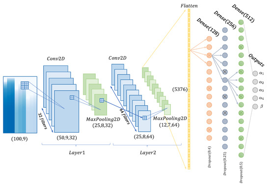
Figure 6.
Sketch of the convolutional neural network (CNN) used in this work.

Table 1.
Convolutional Neural Network structure and parameters used.
- Convolution2D (Conv2D). This corresponds to an image operation based on the application of a given set of filters to enhance specific features of the image. If the input image is A (see Figure 5 with footprint of ) the 2D convolutions of this individual image may be obtained, namely B, by applying the kernel function F, aswhere F stands for the filter applied and ∗ the convolution operator. The operation can be parametrized by using different filter sizes, strides, paddings, activation functions or kernel regularization. Filters of size are intended to highlight specific features in time and space produced by the presence of the dissimilar material region in the mould. Input image dimensions are given by , where for greyscale images, and output image dimensions are calculated by . For instance, the first Conv2D layer in Figure 6 uses a kernel with an input grayscale image object of . This filter operation produces an output image of for this first convolution. Filters normally make use of a certain step, named stride, that move the convolution filter along the x and y axis of the input image. Padding is the parameter which maintains the size of the output images resulting from the convolution B. Keras uses the padding=’same’ technique to avoid image edge trimming. Lastly, when convolution is completed, a ReLu (Rectified Linear Unit ) is used as cut-off function thus avoiding negative outputs that can be generated.
- MaxPooling (MaxPooling2D). This is applied to reduce the dimensions of the convolution filtered images with the purpose of obtaining more efficient and robust characteristics. The model uses a pooling filter, taking the maximum value of the pixels in the neighborhood as the result for a given point. For instance, Figure 6 shows MaxPooling operations used to reduce the image size from to in the first convolution.
- Batch normalization (BatchNormalization). This seeks to alleviate the movements produced in the distributions of internal nodes of the network with the intention of accelerating its training. Those movements are avoided via a normalization step, constraining means and variances of the layer inputs. Furthermore, it reduces the need for dropout, local response normalization and other regularization techniques [23].
- Flatten (Flatten). This operation splits up the characteristics, transforming them and preparing for obtaining a vector-type object [24]. It is used as training input of the subsequent fully-connected neural network (FCNN).
- Dense (Dense). The fully-connected layer is implemented by one or several dense functions. Each layer obtains n inputs from the precedent layer or, in case of the first dense layer, n inputs from the Flatten layer. Then, these inputs are balanced by the neural network weights and bias, and transformed into a set of outputs for the following layer according to their specific activation functions. The final dense layer contains a five-component vector-type to perform the regression on the values of and . Particularly, the neural network used in this work contains three fully connected layers, containing 128, 256 and 512 neurons respectively.
4.2. Training Machine Learning Models
Numerical training experiments started with the pressure probe footprints generated by using mould filling simulations. A set of 3000 images of pressure footprints was used in the CNN model with the purpose of predicting the five variables of position, , size and the relative permeability . Both datasets, pressure probe footprints, as well as the the five variables were already normalized in the interval so no extra treatments were required.
The first step was to split randomly the dataset generated into two pieces usually known as training and test sets. Training and test sets contained all the data in a ratio of 80/20. The test set was qualified as a never-before-seen dataset with the intention to evaluate the model under new data not used during training.
The subsequent step deals with training of the CNN model by using Keras. The network described in the previous section was coded in Keras by a sequential linking of two convolutional layers and three dense layers (see Figure 6 for more details). Each layer applies some tensor operations with the input data, and these operations make use of weight and bias factors. The weight and bias factors are the intrinsic attributes of the different layers used and are considered the parameters where the learning capacity of the network resides. A total of 860,517 parameters was used in the CNN model, Table 1. The determination of the network parameters is carried out by minimization of a norm defined as the sum of the squared differences between the truth values of the variables () and the predicted ones by using the CNN network. This Mean Squared Error (MSE) is used in this work as loss function to minimize ( with N the size of the dataset). The iterative method for minimizing the loss function in combination with a gradient descent called Adadelta were used to this end. The exact rules governing a specific use of gradient descent are defined by the Adadelta [25] Keras optimizer. Training was carried out after not more than 5000 epochs by using 64 as the batch size and lasted around 16 h with a 10 cores Intel Xeon W-2155CPU-3.30 GHz machine. The evolution of training and test losses against the number of epoch training cycles is presented in Figure 7. The best model configuration obtained produces a minimum MSE of after training which was judged accurately enough for modelling purposes.
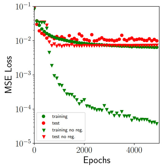
Figure 7.
Training and test MSE (mean square error) losses evolution against the number of epochs training cycles. The data include losses obtained with and without the application of techniques to alleviate overfitting (data augmentation, regularization and dropout).
It is worth highlighting the similarity of MSE loss curves obtained for both training and set datasets which is an indicator of reasonable model performance for unseen data. Highly dissimilar behaviour of these two curves usually indicates overfitting, which is a common problem in machine learning. If the complexity of the network and number of network parameters is too high, not in correspondence with the datasets size, overfitting is produced. In this case, the accuracy obtained after training can be excellent but the error corresponding to the test dataset could be still unacceptable and indicates a deficient model generalization for new unseen data. Several strategies were implemented in this work to alleviate possible overfitting problems according to recommendations found in the literature, namely data-augmentation, regularization and dropout rate in fully-connected layers.
An augmented dataset is generated from the pressure sensor signal by adding a white noise to each image of the training set. The white noise generated follows a normal distribution with zero mean and 0.001 standard deviation. The augmented dataset contains then a total of 14,400 images, with 2400 being from the original set computed with OpenFoam and the remaining 12,000 the augmented one. regularization techniques add a constraining term to the MSE loss function which is proportional, with a regularization factor of , to the total sum of the squared values of the parameters of the network (). Thus, the presence of data outliers is penalized preventing possible overfitting. Lastly, dropout rates were applied in the fully-connected neuron layers, entailing random dropping out, setting to zero, a number of output features of the layer during training producing a less regular structure. The loss curves that correspond to the case without any of the strategies used to alleviate overfitting are also presented in Figure 7. Although the training loss in this case was excellent, and close to , the differences with the test loss were unacceptable. Thus, the model in this case was unable to generalize with the same precision level with new unseen data.
The comparisons between the ground truth values of the variables, , and , and the predicted ones through use of the CNN are gathered in Figure 8. The figure includes both training and test datasets. As a first approximation, the correlation between predicted and ground truth values was fairly good. This was especially true for the position of the dissimilar material region , Figure 8a,b. The network in this situation was able to learn in a highly efficient manner from the given footprint by using only the features associated with the rise up of the pressure signals. However, the accuracy attained for the remaining variables was, in general, more modest although the overall trends were perfectly captured, Figure 8c,d,f. A plausible explanation for this accuracy reduction could be attributed to the similarity of the pressure fields generated by the presence of the dissimilar material region. Two regions defined with similar values of size and/or relative permeability produce very close fluid pressure fields almost indistinguishable, producing nearly no single-valued pressure footprints. This reduction of accuracy was more evident in the case of the relative permeability parameter which is essentially controlled by the pressure gradients. Figure 8e shows the previous statement. Pressure field differences for two small values of may differ only slightly when the macroscopic flow reached the outlet gates, thus producing again almost equal pressure footprints. Nonetheless, the accuracy was judged to be reasonable for the automatic detection of the position and severity of the dissimilar material region.
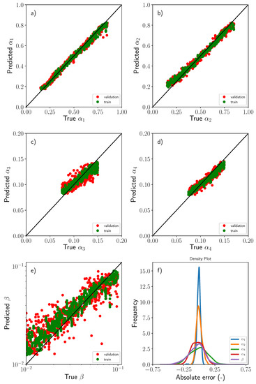
Figure 8.
Comparisons between the ground truth values of the variables, (a) , (b) , (c) , (d) and (e) including training (green) and test (red) data sets, (f) Histograms of the absolute error corresponding to each of the variables used in the regression.
The histograms of the individual absolute errors computed as corresponding to the five variables are also presented in Figure 8f. As mentioned previously, the prediction of the two position variables () was excellent and the error in this case exhibits a Dirac-like type function with of the data lying within an absolute error band of less than . It should be pointed out that the model variables were expressed in non-dimensional and normalized form and thus, the absolute errors were expressed in percentage. The error distribution for the remaining variables was, of course, more flatten and the plausible reasons were discussed previously. The fraction of the total data corresponding to predictions with absolute error lying in the and error band are presented in Table 2 for the sake of completion.
Table 2.
Fraction of the total data with absolute error falling within the and bands.
Figure 9a is presented to illustrate the overall performance of the model. The plots contain some dissimilar material regions selected randomly together with the corresponding predictions by using the test dataset and the sensor network size. As discussed previously, the accuracy of the predictions was fairly good, thus showing the ability of the proposed model to capture the presence of dry regions during liquid moulding.
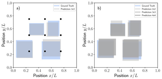
Figure 9.
Comparisons between the ground truth and predictions for five randomly selected dissimilar material regions in terms of position and (a) size for the test data set using the sensor network size, (b) Same results as previously shown but with different sensor network of , and .
The accuracy of the model was also addressed for some additional cases including different pressure network sizes of , (baseline) and corresponding to 4, 9 and 16 equally spaced pressure sensors. It should be noted that as OpenFoam simulations were run a single time, saving the pressure probe evolution at the locations corresponding to each specified network, there was no need for further recalculations. The three models were trained by using the same procedure previously explained and the corresponding MSE losses obtained for the , and networks were 0.016, 0.011 and 0.012, respectively. The MSE losses obtained for the and networks were very similar between them. Such results seem to indicate that the dissimilar material region size used in this study, following the uniform distribution , is perfectly captured even with the network. Increasing the number of sensors to will not result in a better accuracy of the model for such dissimilar material region size. Accordingly, the sensor network size should be previously determined if a minimum dissimilar material size is sought. The predictions for the ground truth cases presented in Figure 9a by using the , and network are now summarized in Figure 9b for the sake of completion.
Lastly, the flow progress predictions for the case presented in Figure 3 are now shown in Figure 10. This case corresponded to a square region centred in , and relative permeability of . The pressure footprint presented in Figure 4a was used as input to predict the position, size and relative permeability yielding the 5-tuple from the ground truth values of . OpenFoam simulations were run subsequently and the corresponding flow patterns gathered in Figure 10. The agreement between the ground truth flow patterns shown in Figure 3 and the predicted ones was excellent, MSE, considering that the only information used comes from a discrete network of pressure sensors.
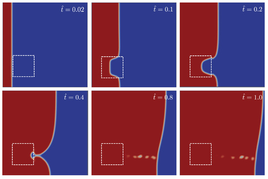
Figure 10.
Snapshots of the flow progress through the mould for different non-dimensional times = 0.02, 0.2, 0.4, 0.8 and 1.0 corresponding to the predicted values for the case shown in Figure 3. Flow progress from left to right. Red and blue colours correspond to phase values of and , respectively. For the sake of clarity, white dashed lines corresponding to the dissimilar material region were superimposed.
4.3. Deploying Machine Learning Models
The CNN model and the weights resulting after training were saved for subsequent predictions with new unseen data that could come, for instance, from the manufacturing laboratory. To this end, the model architecture and the corresponding weights were stored by using json format (JavaScript Object Notation) and hdf5 Hierarchical Data Format (HDF) respectively. Once the network was trained, it could be deployed subsequently and evaluated at any time by loading the model, weights and the new unseen data without the need of retraining.
5. Discussion
Model Robustness
The previous section was devoted to describing a new machine learning model to detect automatically the presence of a dissimilar material region during manufacturing of composites by liquid moulding. Examination of the model architecture, training procedure, accuracy and the ability to generalize a response under new unseen data was analyzed in detail. However, a deeper assessment of its robustness should be conducted to address other relevant effects and uncertainties that could potentially arise during the manufacturing process. Among others, these involve the presence of increasing pressure signal noise, as well as possible sensor malfunctions or the size of the sensor array used. Additionally, the response of the trained model through use of different type of unseen data was evaluated. For instance, the response to other dissimilar material region shapes instead of a rectangular one, the rectangle size out of the distribution used for training, as well as the presence of simultaneous regions during filling, will be analyzed.
As described previously, a white noise signal following a Gaussian distribution was originally superposed on the pressure footprints to improve the overfitting response of the model and its capability to generalize for new unseen data inputs. Once the model was trained, the prediction ability with white noise corrupted data was checked. Figure 11a shows the pressure evolution corresponding to the nine sensors installed in the model with white noise of for the case presented in Figure 4a. Such corrupted signals were used to determine the lack of accuracy due to the presence of noise and the results presented in Figure 11b in terms of MSE. It was evident that for increasing noise standard deviation, some of the pressure signals may overlap hampering the adequate prediction of the model. It should be pointed out again, that the main sources of model deviations from ground truth values were related to the , and variables, and more specifically to related with the permeability. Unsurprisingly, the position of the dissimilar material region was still well predicted by the model even if the noise signal level was increased.
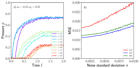
Figure 11.
(a) Corrupted pressure signal with white noise following the Gaussian distribution , (b) MSE as a function of white noise standard deviation .
Another possible source of lack of prediction capacity of the model is sensor malfunction. During manufacturing, it is not unusual that sensor signals can be lost due to a malfunction problem or inadequate wiring. In this case, if a sensor signal is lost from the early beginning of the test, the sensor footprint image will be undoubtedly altered creating a zero-pressure reading in the columns presented in Figure 5a. Under such circumstances, the trained model was not able to recognize the new patterns created by the signal lost and the accuracy of the model was destroyed. Although this can be considered an important shortcoming of the model, it can be easily circumvented if the network is previously trained with data including a signal lost which is time inexpensive for the limited number of sensors used. For instance, pressure footprint datasets used for the network can be trained removing one of the sensor readings leading to a size images rather than the baseline ones.
Figure 12 shows the robustness of the trained model against new unseen data with a structure different than those data used for training. For this exercise, the model was evaluated by using pressure signals obtained with circular dissimilar material regions, see Figure 12a and double size rectangle regions following the distributions, see Figure 12b. Although the geometry used in these two cases produced, of course, different pressure footprints than those used for training of the baseline problem, the results obtained from the model were still reasonable in location and area indicating an adequate detection of specific patterns even if non-standard images are used.
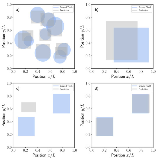
Figure 12.
Comparisons between the ground truth and predictions for different dissimilar material realizations: (a) Circular, (b) Double size rectangular, (c) Two equal rectangles, (d) Two equal rectangles with CNN model trained with a new double rectangle data set.
The case of two rectangular regions deserves additional and specific comments. In this case, two equal rectangle dissimilar material regions were generated randomly but assuming centered x-y symmetry so the problem variables used for the regression remain the same, Figure 12c. Independent pressure footprints corresponding to two rectangle problems were generated with OpenFoam and the baseline model with a sensor network size was used to predict the position of an unique equivalent dissimilar material region. Unfortunately, in this case, the response was misleading and the model was unable to detect the specific features of this outlier case. The prediction of the model was obviously a single rectangular region that neither matches the averaged position nor the area of the two input rectangles, Figure 12c. As mentioned previously, such problems were easily circumvented by additional training of the CNN model with the new data set corresponding to 3000 random realizations of the two rectangular dissimilar material regions. The CNN was trained again and the new predictions presented in Figure 12d for the same individual case presented in c. Now, the model was able to detect perfectly the two rectangles with a precision level meeting the expectations (see error histograms in Figure 8f). This simple exercise demonstrated the prediction capability of the CNN architecture trained with the appropriate dataset.
6. Conclusions and Final Remarks
A supervised regression machine learning model based on a convolutional neural network is presented in this work to predict the position, size and relative permeability of a dissimilar material region inside a square mould subjected to a macroscopic one dimensional flow in liquid moulding. The presence of the dissimilar material region produces distortions of the pressure field and flow patterns which can be detected by a discrete network of sensors equally distributed over the mould surface. The use of a fully-based experimental approach to build machine learning models in materials manufacturing would be challenging due to cost factors. To avoid this issue, dataset augmentation based on simulations becomes crucial to success. This was the approach used in this paper which makes use of extensive modelling of mould filling through use of OpenFoam as the fluid mechanics solver.
The forward model described in the paper is able to generate the pressure probes evolution during the filling time and these data were properly stored as a pressure footprints. A total of 3000 random realizations for the five variables describing the position, size and relative permeability of a rectangular dissimilar region were generated by computer. The inverse problem to predict the five variables from the regression of the individual pressure footprints was based on the use of a convolutional neural network which was able to learn from specific features of the artificial images generated. The CNN had two sequential convolutional layers and three fully-connected neuron layers to relate the pressure footprints with the corresponding position, size and relative permeability of the dissimilar material regions. The model architecture and training were implemented in Keras, a high-level neural network API. The determination of the network parameters was carried out by minimizing the mean square error loss over an increasing number of epochs. Training was carried out by using some numerical strategies to alleviate overfitting, producing a model able to generalize the response under new unseen data not used during training. The model yielded excellent accuracy for the center position of the dissimilar material region while the one corresponding to its size and relative permeability was good but more modest as shown in the error histograms distribution in Figure 8f. Taking into account the difficulties and scatter associated with the permeability measurement, the accuracy attained by the model was judged to be coherent with the experimental limitations. Lastly, the model robustness against new data with structure not used during training is analyzed in detail. In addition, the effects of sensor malfunctions, noise signals, presence of simultaneous dissimilar regions, different shapes among others were studied. It should be remarked that the purpose of this work was to establish a general framework for fully-synthetic-trained machine learning models to address the occurrence of manufacturing disturbances without placing emphasis on its performance, robustness and optimization. In summary, the following conclusions can be drawn:
- Machine learning and artificial intelligence strategies open revolutionary opportunities in material science and, more specifically, in materials and parts manufacturing. The ability of these technologies to deal and overcome complex physical and engineering problems that relate different datasets, as sensors and dissimilar material regions in this work, is highly aligned with Industry 4.0 concepts. In the future, this will enable the development of efficient cyber-physical systems to detect defects automatically during manufacturing while guaranteeing the implementation of the appropriate corrective actions.
- Some of the major concerns and drawbacks of the application of machine learning methods in manufacturing of structural composites are related with enormous costs and development times associated with the experimental generation of the large datasets required for training. A way of easing the burden on experimental tasks is to involve the cooperative help of simulation results to create augmented datasets. Of course, it could be argued that the accuracy of processing simulation tools to predict the involved variables is dubious, specially if manufacturing disturbances should be taken into account. This paper has presented a fully simulation-based machine learning model, although the purpose in future implementations will be to combine both experimental and model datasets.
- Many modelling techniques involve machine learning algorithms and include different architectures and methods. It should be noted that similar or even better results could be obtained by using other approaches not examined here. The aim of the paper was not to provide the optimum model configuration but to analyze the ability of machine learning to detect automatically flow disturbances occurring during liquid moulding by testing a simple problem. A future objective will entail examining of integration into a complete system able to detect manufacturing disturbances while implementing automatically the required corrective actions to maintain a constant quality of the manufactured part.
Author Contributions
Conceptualization, C.G. and J.F.-L.; methodology, C.G. and J.F.-L.; software, C.G. and J.F.-L.; validation, C.G. and J.F.-L.; formal analysis, C.G. and J.F.-L.; investigation, C.G. and J.F.-L.; resources, C.G.; data curation, C.G. and J.F.-L.; writing–original draft preparation, J.F.-L; writing–review and editing, C.G.; visualization, C.G. and J.F.-L.; supervision, C.G.; project administration, C.G.; funding acquisition, C.G. All authors have read and agreed to the published version of the manuscript.
Funding
This research was funded by the Regional Government of Madrid through the research and innovation Innovation Hubs 2018 TEMACOM project.
Conflicts of Interest
The authors declare no conflict of interest.
References
- González, C.; Vilatela, J.; Molina-Aldareguía, J.; Lopes, C.; LLorca, J. Structural composites for multifunctional applications: Current challenges and future trends. Prog. Mater. Sci. 2017, 89, 194–251. [Google Scholar] [CrossRef]
- Llorca, J.; González, C.; Molina-Aldareguía, J.; Segurado, J.; Seltzer, R.; Sket, F.; Rodríguez, M.; Sádaba, S.; Muñoz, R.; Canal, L. Multiscale modeling of composite materials: A roadmap towards virtual testing. Adv. Mater. 2011, 23. [Google Scholar] [CrossRef] [PubMed]
- Roth, Y.C.; Weinholdt, M.; Winkelmann, L. Liquid Composite Moulding - Enabler for the automated production of CFRP aircfraft components. In Proceedings of the 16th European Conference on Composite Materials, ECCM 2014, Seville, Spain, 22–26 June 2014; pp. 22–26. [Google Scholar]
- Advani, S.; Hsiao, K.T. (Eds.) 1—Introduction to composites and manufacturing processes. In Manufacturing Techniques for Polymer Matrix Composites (PMCs); Woodhead Publishing Series in Composites Science and Engineering; Woodhead Publishing: Sawston, UK, 2012; pp. 1–12. [Google Scholar] [CrossRef]
- Rudd, C.D.; Long, A.C.; Kendall, K.N.; Mangin, C.G.E. Liquid Moulding Technologies; Woodhead Publishing: Sawston, UK, 1997. [Google Scholar] [CrossRef]
- Siddig, N.A.; Binetruy, C.; Syerko, E.; Simacek, P.; Advani, S. A new methodology for race-tracking detection and criticality in resin transfer molding process using pressure sensors. J. Compos. Mater. 2018, 52, 4087–4103. [Google Scholar] [CrossRef]
- Zhou, B.; Lapedriza, A.; Xiao, J.; Torralba, A.; Oliva, A. Learning deep features for scene recognition using places database. Adv. Neural Inf. Process. Syst. 2014, 1, 487–495. [Google Scholar]
- Xiao, J.; Hays, J.; Ehinger, K.A.; Oliva, A.; Torralba, A. SUN database: Large-scale scene recognition from abbey to zoo. In Proceedings of the IEEE Computer Society Conference on Computer Vision and Pattern Recognition, San Francisco, CA, USA, 13–18 June 2010; pp. 3485–3492. [Google Scholar] [CrossRef]
- Mezzasalma, S.A. Chapter Three The General Theory of Brownian Relativity. Interface Sci. Technol. 2008, 15, 137–171. [Google Scholar] [CrossRef]
- Bock, F.E.; Aydin, R.C.; Cyron, C.J.; Huber, N.; Kalidindi, S.R.; Klusemann, B. A review of the application of machine learning and data mining approaches in continuum materials mechanics. Front. Mater. 2019, 6. [Google Scholar] [CrossRef]
- Wu, J.; Yin, X.; Xiao, H. Seeing permeability from images: Fast prediction with convolutional neural networks. Sci. Bull. 2018, 63, 1215–1222. [Google Scholar] [CrossRef]
- Iglesias, M.; Park, M.; Tretyakov, M.V. Bayesian inversion in resin transfer molding. Inverse Probl. 2018, 34, 1–49. [Google Scholar] [CrossRef]
- Lähivaara, T.; Kärkkäinen, L.; Huttunen, J.M.J.; Hesthaven, J.S. Deep convolutional neural networks for estimating porous material parameters with ultrasound tomography. J. Acoust. Soc. Am. 2018, 143, 1148–1158. [Google Scholar] [CrossRef] [PubMed]
- Zhu, Y.; Zabaras, N. Bayesian deep convolutional encoder–decoder networks for surrogate modeling and uncertainty quantification. J. Comput. Phys. 2018, 366, 415–447. [Google Scholar] [CrossRef]
- Bruschke, M.V.; Advani, S.G. A finite element/control volume approach to mold filling in anisotropic porous media. Polym. Compos. 1990, 11, 398–405. [Google Scholar] [CrossRef]
- Bruschke, M.V.; Advani, S.G. A numerical approach to model non-isothermal viscous flow through fibrous media with free surfaces. Int. J. Numer. Methods Fluids 1994, 19, 575–603. [Google Scholar] [CrossRef]
- Weller, H.G.; Tabor, G.; Jasak, H.; Fureby, C. A tensorial approach to computational continuum mechanics using object-oriented techniques. Comput. Phys. 1998, 12, 620–631. [Google Scholar] [CrossRef]
- Deshpande, S.S.; Anumolu, L.; Trujillo, M.F. Evaluating the performance of the two-phase flow solver interFoam. Comput. Sci. Discov. 2012, 5, 014016. [Google Scholar] [CrossRef]
- PyDOE. The Experimental Design Package for Python. Available online: https://pythonhosted.org/pyDOE/ (accessed on 9 June 2020).
- Chollet, F.; KERAS. Available online: https://github.com/fchollet/keras (accessed on 9 June 2020).
- Cun, Y.L.; Boser, B.; Denker, J.S.; Howard, R.E.; Habbard, W.; Jackel, L.D.; Henderson, D. Handwritten Digit Recognition with a Back-propagation Network. In Advances in Neural Information Processing Systems 2; Morgan Kaufmann Publishers Inc.: San Francisco, CA, USA, 1990; pp. 396–404. [Google Scholar]
- LeCun, Y.; Bengio, Y.; Hinton, G. Deep learning. Nature 2015, 521, 436–444. [Google Scholar] [CrossRef]
- Ioffe, S.; Szegedy, C. Batch normalization: Accelerating deep network training by reducing internal covariate shift. arXiv 2015, arXiv:1502.03167. [Google Scholar]
- Jin, J.; Dundar, A.; Culurciello, E. Flattened convolutional neural networks for feedforward acceleration. arXiv 2014, arXiv:1412.5474. [Google Scholar]
- Zeiler, M.D. ADADELTA: An Adaptive Learning Rate Method. arXiv 2012, arXiv:abs/1212.5701. [Google Scholar]
© 2020 by the authors. Licensee MDPI, Basel, Switzerland. This article is an open access article distributed under the terms and conditions of the Creative Commons Attribution (CC BY) license (http://creativecommons.org/licenses/by/4.0/).