Thermal Buckling Behaviour of Thin and Thick Variable-Stiffness Panels

Abstract

The possibility of designing composite panels with non-uniform stiffness properties offers a chance for achieving highly-efficient configurations. This is particularly true for buckling-prone structures, whose response can be shaped through a proper distribution of the membrane and bending stiffnesses. The thermal buckling behaviour of composite panels is among the aspects that could largely benefit from the adoption of a variable-stiffness design, but, in spite of that, it has rarely been addressed. The paper illustrates a semi-analytical approach for evaluating the thermal buckling response of variable-stiffness plates (VSP) by considering different boundary conditions. The formulation relies upon the method of Ritz and a variable-kinematic approach, leading to a computationally efficient implementation, which is particularly useful for exploring the larger design spaces, typical of variable-stiffness configurations. Due to the possibility of choosing the underlying kinematic approach as an input of the analysis, the formulation is not restricted to thin plates, but is suitable for analyzing the response of thick plates as well. Novel results are derived, which can be useful for benchmarking purposes and for gathering insight into the mechanical behaviour of variable-stiffness plates. Furthermore, the importance of transverse shear flexibility is illustrated with respect to the boundary conditions as well as the degree of steering of the fibers.

1. Introduction

Thermal buckling phenomena are of crucial importance in the design of aerospace structures [1]. High-speed aircraft and launch vehicles’ structural elements are indeed exposed to aerodynamic heating that may promote elastic instability phenomena. In some cases, such as for cryogenic launch vehicles, the source of internal forces leading to instability is due to low temperatures, and cooling-induced buckling should be considered during the design process. With these motivations, thermal buckling has been the subject of many investigations in the aerospace structural community. In this context, an important role is played by rectangular plates that, despite their simplicity, are often a good approximation, at least in a early design phases, of sub-portions of more complex structural topologies. For instance, the portion of skin between stringers and frames can be assumed as a rectangular plate subjected to ideal constraints along the boundaries. Another advantage of analyzing idealized plate-like structures lies in the possibility of gathering insight into the underlying structural mechanics in a clear and straightforward manner, obtaining design guidelines that can be extended even to more complex structures.

Thermal buckling of composite plates was analyzed, in several past works, referring to Classical Lamination Theory (CLT) [2,3,4,5,6], as well as First-Order Shear Deformation Theory (FSDT) [7]. In some cases, higher-order approaches [8,9,10,11] and 3D solutions [12,13] were formulated for extending the analysis capabilities to thick plates and sandwich structures.

The tailoring opportunities offered by composite materials can be further improved by allowing the orientation of the fibers to vary locally, according to the desired load path to be achieved. This chance has been known for a long time, with the first scientific paper mentioning this topic dating back to almost 50 years ago [14]. The lack of available technologies hindered the progress of this concept until the early 1990s, when the pioneering studies of Leissa and Martin [15], Hyer [16,17] and Gürdal [18] increased interest in the concept of variable-stiffness structures. In the past several years, drastic improvements in the manufacturing techniques allowed variable-stiffness constructions to become a hot topic and suitable candidates for the aerostructures of the next generation. Theoretical investigations and numerical models were carried out for analyzing their buckling [19,20,21] and post-buckling [22,23,24] response, in most cases referring to thin plate theory or FSDT [25]. Refined theories have been less commonly employed: the free vibration response of variable-stiffness plates (VSP) is investigated in [26,27] using finite elements, while the authors presented a variable-kinematics, Ritz-based procedure for buckling and free-vibration analysis [28] of VSP based on Carrera’s Unified Formulation (CUF) [29,30,31]. Tornabene and co-workers discussed the application of variable-kinematics approaches for analyzing the modal and static response of variable-stiffness laminates [32,33] and sandwich constructions [34,35].

Recently, the thermal buckling behaviour of variable-stiffness plates was investigated in [36], using a thin-plate finite element formulation, and [37], by considering FSDT. Thermally induced multi-stable configurations were assessed by Haldar et al. [38] using finite elements and the Ritz approach proposed by Dano and Hyer [39].

To the best of the author’s knowledge, no previous attempts could be found in the literature to analyze the thermal buckling of VSP using refined theories. The present work aims at filling this gap by presenting a unified Ritz-based modeling framework, where the analyst has the possibility of choosing the underlying plate theory—both as equivalent single layer (ED) or layer-wise (LD)—so that both thin and thick plate configurations can be studied.

Furthermore, novel closed-form solutions are presented for the evaluation of pre-buckling internal stress distribution, which can be successfully employed for gathering further understanding into the mechanical response of VSP, as well as improving the efficiency of the buckling solution procedure.

2. Theoretical Framework

This work is devoted to the thermal buckling analysis of variable-stiffness composite plates, i.e., flat plates characterized by the stacking of plies with non-straight fibers.

Several laws were proposed in the literature for describing the orientation of the fibers within the panel domain, including linear and nonlinear ones [20,25,40]. Linear variation of the orientation angle is considered here due to its effectiveness in allowing the description of a variable-stiffness ply by means of two parameters only. This choice tends to limit the design space with respect to more general nonlinear descriptions, but it appears useful when trying to condense the behaviour of VSP in design charts or compact summary tables, as done in this study. In other words, the understanding of the mechanical response of VSP, their potential for elastic tailoring, as well as the main features associated with their analysis can be grasped even by restricting the focus to the case of fiber linear variation.

The plates are characterized by planar dimensions $a\times b$, where a denotes the longitudinal direction along the x-axis and b is the transverse direction parallel to the y-axis, as illustrated in Figure 1. The total thickness is denoted with h.

According to the notation adopted here, a ply denoted with $<{\theta }_0|{\theta }_1{>}_x$ is characterized by a fiber variation along the x-axis, where ${\theta }_0$ is the orientation, measured with respect to the x-axis, at the plate center, and ${\theta }_1$ the one at the plate edge (see Figure 1a). Similarly, steering of the fibers along the direction y is denoted with $<{\theta }_0|{\theta }_1{>}_y$ (see Figure 1b). Starting from the fiber passing through the plate center, the other ones are obtained by translation of the reference fiber along the x- or y-direction, referring to a strategy sometimes denoted as a shifted method [26,41].

By considering fiber variation along the x-direction, the orientation angle at a generic point is given as:

$$\theta \left(x,y\right)=\frac{2\left({\theta }_1-{\theta }_0\right)}{a}\left|x\right|+{\theta }_0.$$

(1)

An analogous linear law is obtained when variation takes place along the y-direction. Referring to common design rules of the aerospace industry, the stacking sequence is taken as symmetric with respect to the midplane, i.e., a layer oriented at $<{\theta }_0|{\theta }_1>$ at the distance $\overline{z}$ from the plate midplane implies the presence of another identical layer at the distance $-\overline{z}$. In addition, the analysis is restricted to the case of balanced laminates, meaning that a ply at $<{\theta }_0|{\theta }_1>$ requires the presence of another ply at $-<{\theta }_0|{\theta }_1>$ at any position in the stack.

2.1. Variational Formulation and Approximate Solution

A variable-kinematic approach is considered due to the possibility of analyzing wide ranges of plate configurations. Specifically, the underlying framework refers to the well-known Carrera’s Unified Formulation (CUF) (see, for instance, [29,42,43]), offering the advantage of allowing a relatively easy implementation, which is independent from the kinematic model to be used for the structural analysis. Indeed, the theory is defined as an input of the problem, and can be chosen among the class of Equivalent Single Layer (ED) and Layer-Wise (LD) formulations.

The formulation is developed in the context of a displacement-based approach, where the three displacement components are the unknowns of the problem. The buckling condition is sought by application of the Trefftz criterion, which is written as:

$$\delta \left({\delta }^2\Pi \right)=0,$$

(2)

where ${\delta }^2\Pi$ is the quadratic part of the Taylor expansion of the total potential energy, whose expression is given as:

$${\delta }^2\Pi =\frac{1}{2}\sum _{k=1}^{N_l}{\int }_{\Omega }{\int }_{z_k}^{z_{k+1}}\left({\mathit{ϵ}}_p^{k^T}{\mathit{\sigma }}_p^k+{\mathit{ϵ}}_n^{k^T}{\mathit{\sigma }}_n^k+{\mathit{ϵ}}_{p_{nl}}^{k^T}{\mathit{\sigma }}_{p0}^k\right)\mathrm{d}z\mathrm{d}\Omega ,$$

(3)

where $\Omega$ denotes the domain $[-a/2a/2]\times [-b/2b/2]$, and k is the ply-related index. Note that the first five contributions entering the right-hand side of Equation (3) should be intended as variations with respect to the equilibrium condition, whilst the last one, ${\mathit{\sigma }}_{p0}^k$ , defines the membrane stress state obtained from the pre-buckling analysis.

The components of the deformation and stress tensors reported in Equation (3), in the case of a generic 3D elasticity formulation of the problem, are split into the in-plane and normal contributions, according to the definitions:

$${\mathit{ϵ}}_p^k={\left\{{\mathit{ϵ}}_{xx}^k{\mathit{ϵ}}_{yy}^k{\gamma }_{xy}^k\right\}}^{\mathrm{T}},{\mathit{\sigma }}_p^k={\left\{{\mathit{\sigma }}_{xx}^k{\mathit{\sigma }}_{yy}^k{\tau }_{xy}^k\right\}}^{\mathrm{T}},$$

(4)

$${\mathit{ϵ}}_n^k={\left\{{\gamma }_{xz}^k{\gamma }_{yz}^k{\mathit{ϵ}}_{zz}^k\right\}}^{\mathrm{T}},{\mathit{\sigma }}_n^k={\left\{{\tau }_{xz}^k{\tau }_{yz}^k{\mathit{\sigma }}_{zz}^k\right\}}^{\mathrm{T}},$$

(5)

while the pre-buckling membrane stresses are:

$${\mathit{\sigma }}_{p0}^k={\left\{{\mathit{\sigma }}_{0xx}^k{\mathit{\sigma }}_{0yy}^k{\tau }_{0xy}^k\right\}}^{\mathrm{T}}.$$

(6)

The strain components in work-conjugacy relation with those of Equation (6) are the nonlinear part of the Green–Lagrange strain tensor, which is given by:

$$\begin{array}{c}\hfill {\mathit{ϵ}}_{p_{nl}}^k=\left\{\begin{array}{c}\frac{1}{2}\left(u_{,x}^{k^2}+v_{,x}^{k^2}+w_{,x}^{k^2}\right)\\ \frac{1}{2}\left(u_{,y}^{k^2}+v_{,y}^{k^2}+w_{,y}^{k^2}\right)\\ u_{,x}^k{u}_{,y}^k+v_{,x}^k{v}_{,y}^k+w_{,x}^k{w}_{,y}^k\end{array}\right\}.\end{array}$$

(7)

The functional of Equation (3) can be expressed as a function of the displacement vector ${\mathit{u}}^k={\left\{u^k{v}^k{w}^k\right\}}^{\mathrm{T}}$ after introducing the constitutive law, in this case taken as the generalized Hooke’s Law in 3D for an orthotropic material. The approximate solution is sought here referring to the Ritz method. The procedure is briefly outlined in the following, and the interested reader is referred to [28,44,45,46,47,48] for more details.

According to the CUF formalism, the displacement components are expanded as the product of thickness functions $F_{\tau }$ and generalized displacement components ${\mathit{u}}_{\tau }^k$ as:

$${\mathit{u}}^k\left(\xi ,\eta ,\zeta \right)=F_{\tau }\left(\zeta \right){\mathit{u}}_{\tau }^k\left(\xi ,\eta \right),$$

(8)

where $\xi$ and $\eta$ are non-dimensional in-plane coordinates, defined as $\xi ={\displaystyle \frac{2x}{a}}$, $\eta ={\displaystyle \frac{2y}{b}}$ and defined in the bi-unitary domain $[-11]\times [-11]$.

The thickness functions of Equation (8) are taken as simple polynomials and a combination of Legendre polynomials in the case of Equivalent Single Layer and Layer-wise theories, respectively.

Following the classical Ritz scheme, the generalized displacement components ${\mathit{u}}_{\tau }^k$ are represented as the linear superposition of an arbitrary number of trial functions:

$$u_{r\tau }^k\left(\xi ,\eta \right)=N_{r\tau i}\left(\xi ,\eta \right)c_{r\tau i}^k,$$

(9)

where summation is implied with respect to the index i, whilst r defines the generic displacement component. The coefficients $c_{r\tau i}^k$ are the unknown Ritz amplitudes, and the trial function $N_{r\tau i}$ reads:

$$N_{r\tau i}=f_{r\tau }\left(\xi \right)p_m\left(\xi \right)g_{r\tau }\left(\eta \right)p_n\left(\eta \right),$$

(10)

where $p_i$ are Chebyshev polynomials, while f and g are polynomial boundary functions (for a definition, see [49]).

After substituting Equation (9) into the functional given by Equation (3), and applying the criterion given by Equation (2), the set of discrete equations governing the buckling response is obtained as:

$$\left(\mathit{K}+\lambda \mathit{G}\right)\mathit{c}=\mathbf{0},$$

(11)

where $\mathit{K}$ and $\mathit{G}$ are the linear and the geometric stiffness matrices, respectively. The scalar $\lambda$ is the buckling multiplier, and is obtained as the smallest magnitude eigenvalue of the eigenproblem established by Equation (11). In the context of thermal buckling analysis, it is generally of interest to identify the smallest positive and negative eigenvalues, in order to obtain the critical temperatures associated with heating and cooling. In some cases, all of the eigenvalues have the same sign, thus instability is possible only for cooling or heating.

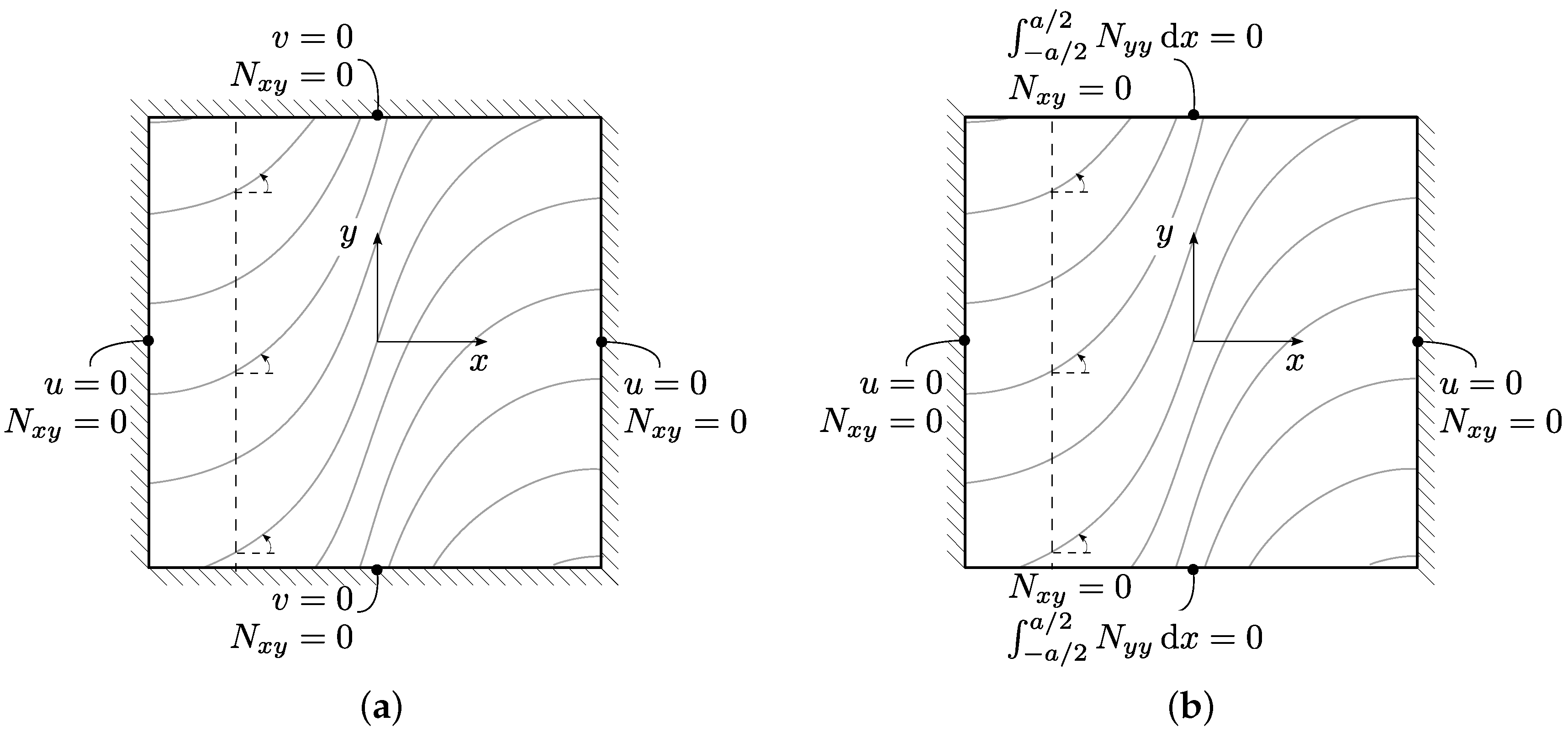
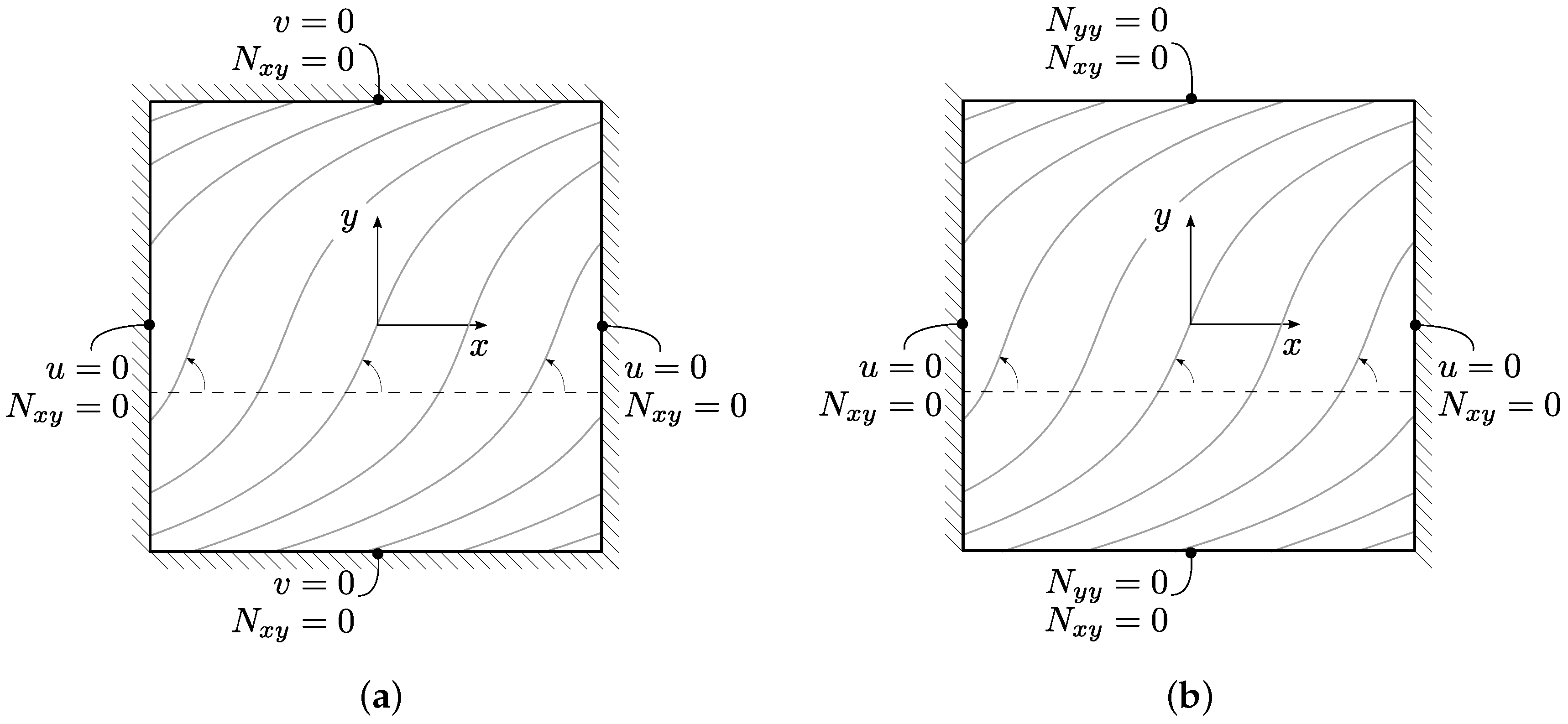
2.2. Pre-Buckling Solutions

The geometric stiffness matrix $\mathit{G}$ depends on the membrane pre-buckling stresses, whose evaluation represents the first step of the overall buckling procedure. To this aim, closed-form solutions are derived for establishing the state of pre-buckling internal forces—to the best of the author’s knowledge, they were not previously available in the literature—for four sets of boundary conditions. The conditions under investigation are summarized in Figure 2 and Figure 3. According to the nomenclature adopted hereinafter, the term Case-Txi specifies a configuration characterized by fiber variation along the x-axis, and i is equal to: 1 if all the four edges are restrained against the expansion/contraction along the direction normal to the plate edge; 2 if only the longitudinal edges are prevented from the movement along the direction normal to the plate edges. Similarly, Case-Tyi conditions are relative to two possible cases associated with fiber variation along y.

The approach for deriving the pre-buckling, thermally-induced stresses refers to classical membrane theory of laminated plates. Under the assumptions introduced here in terms of stacking sequence and boundary conditions, the solution are exact for a generic 3D laminate. Similar results, but restricted to the purely elastic case, can be found in [50].

2.2.1. Thermoelastic Strains and Constitutive Relation

Following the classical approach adopted in thermoelastic analysis of laminates [51], the vector of membrane strains can be organized as:

$${\mathit{ϵ}}^{\mathrm{tot}}={\mathit{ϵ}}^{\mathrm{th}}+{\mathit{ϵ}}^{\mathrm{m}},$$

(12)

where the superscript ${\mathit{ϵ}}^{\mathrm{tot}}$ is the total deformation, which is represented as the sum of a contribution due to thermal and mechanical strains, ${\mathit{ϵ}}^{\mathrm{th}}$ and ${\mathit{ϵ}}^{\mathrm{m}}$. With respect to Equation (4), the subscript p is now omitted.

Assuming linear thermoelastic behaviour, the thermally-induced strains are expressed as:

$${\mathit{ϵ}}^{\mathrm{th}}=\widehat{\mathit{\alpha }}\Delta T,$$

(13)

having indicated with $\Delta T$ a temperature variation, taken positive for heating, with respect to the stress-free reference condition, and $\widehat{\mathit{\alpha }}$ the vector collecting the laminate coefficients of thermal expansions, which are obtained as:

$$\widehat{\mathit{\alpha }}={\mathit{A}}^{-1}{\widehat{\mathit{N}}}^{\mathrm{th}}=\mathit{a}{\widehat{\mathit{N}}}^{\mathrm{th}},$$

(14)

where $\mathit{A}$ is the well-known membrane stiffness matrix, and its inverse $\mathit{a}={\mathit{A}}^{-1}$ is the membrane compliance. The unit thermal stress resultant ${\widehat{\mathit{N}}}^{\mathrm{th}}$ of Equation (14) can obtained as [51]:

$${\widehat{\mathit{N}}}^{\mathrm{th}}=\sum _k{\int }_{z_k}{\mathit{Q}}^k{\mathit{\alpha }}^k\mathrm{d}z.$$

(15)

Recalling now the constitutive equation of a symmetrically layered membrane:

$$\mathit{N}=\mathit{A}\left({\mathit{ϵ}}^{\mathrm{tot}}-{\mathit{ϵ}}^{\mathrm{th}}\right)$$

(16)

and inverting Equation (16) and using Equation (15),

$${\mathit{ϵ}}^{\mathrm{tot}}=\mathit{a}\mathit{N}+\widehat{\mathit{\alpha }}\Delta T$$

(17)

is obtained, which provides an expression for the total strains in terms of membrane forces and temperature variation.

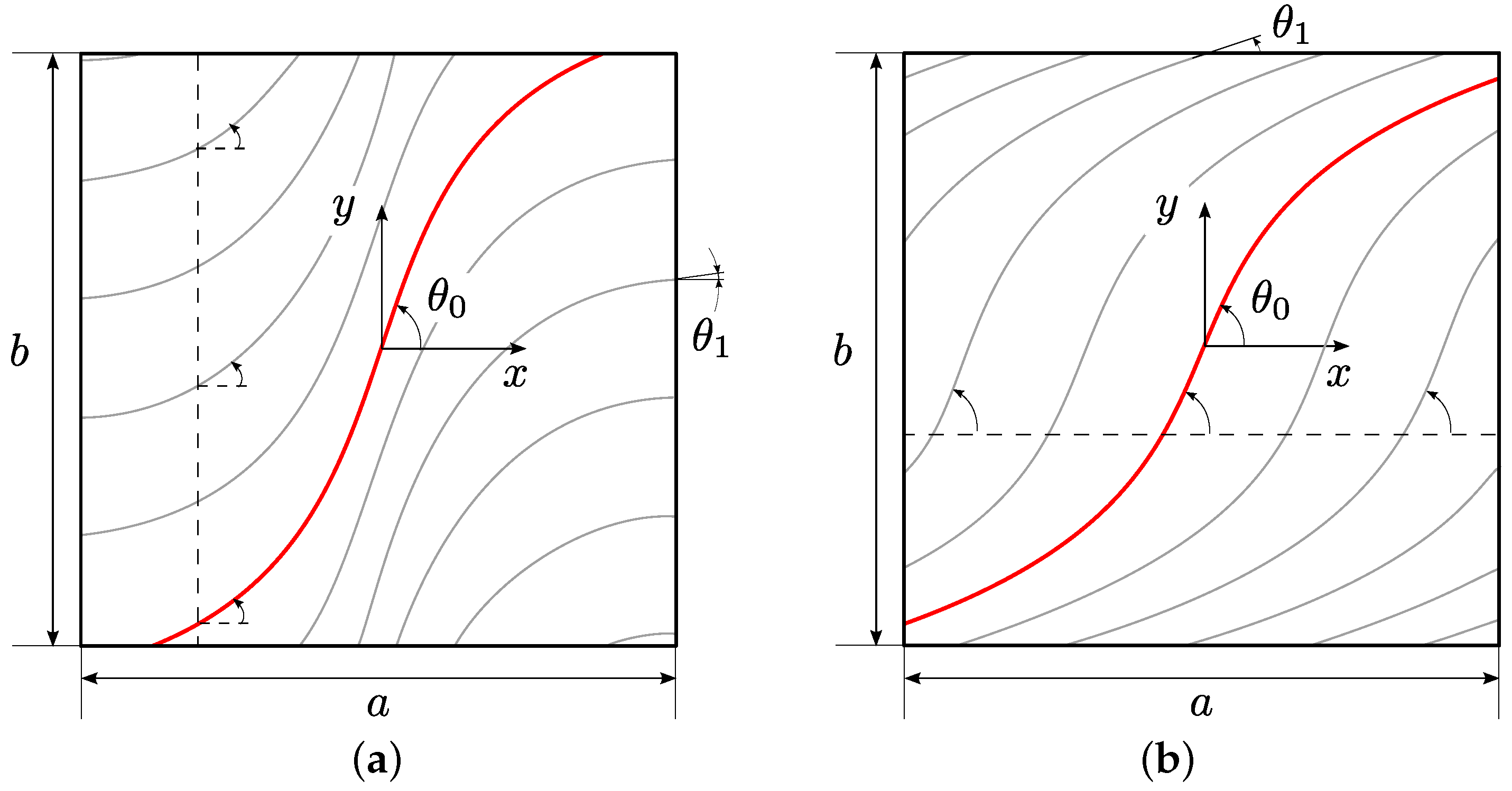
2.2.2. Semi-Inverse Approach

The pre-buckling problem is solved by means of a semi-inverse approach, where the initial assumption regards the shear membrane force per unit length $N_{xy}$, which is taken identically null inside the plate domain and along its boundaries, i.e., $N_{xy}=0$. The closed-form solutions for $N_{xx}$ and $N_{yy}$ are then derived by enforcing the fulfillment of the equilibrium equations and the kinematic and equilibrium conditions at the boundaries. The final step of the approach consists of verifying the compatibility of the solution, providing a proof that the resulting solution is indeed the exact solution of the linear elastic pre-buckling problem.

The in-plane pre-buckling equations, which are uncoupled from the out-of-plane one due to the assumption of symmetric laminate, are given as:

$$\left\{\begin{array}{c}{N}_{xx,x}+N_{xy,y}=0,\hfill \\ N_{yy,y}+N_{xy,x}=0.\hfill \end{array}\right.$$

(18)

Starting from the tentative solution characterized by $N_{xy}=0$, it is seen, from Equation (18), that the equilibrium equations reduce to:

$$\left\{\begin{array}{c}{N}_{xx,x}=0\hfill \\ N_{yy,y}=0\hfill \end{array}\right.\Rightarrow \left\{\begin{array}{c}{N}_{xx}=N_{xx}\left(y\right),\hfill \\ N_{yy}=N_{yy}\left(x\right),\hfill \end{array}\right.$$

(19)

meaning that the direct membrane forces are a function of one single coordinate.

Depending on the essential conditions at the boundaries, which are discussed next, and starting from the equilibrium requirement given by Equation (19), it is possible to determine the pre-buckling solution. The resulting internal force distribution is verified ex-post to be respectful of the compatibility condition, which is given by:

$${\mathit{ϵ}}_{xx,yy}+{\mathit{ϵ}}_{yy,xx}={\gamma }_{xy,xy}.$$

(20)

Note that Equation (20) can be written in terms of force resultants $N_{ik}$ after expressing the strain components ${\mathit{ϵ}}_{xx}$, ${\mathit{ϵ}}_{yy}$ and ${\gamma }_{xy}$ as function of the laminate membrane compliance coefficients.

It is noted that all the solutions derived next do satisfy equilibrium and compatibility conditions, although the verifications of Equation (20) are omitted here for the sake of brevity.

2.2.3. Case-Tx1

The first set of conditions is illustrated in Figure 2a, and is relative to a VSP with fibers varying along the direction x. The in-plane conditions are such that normal displacements at the boundaries are zero. Recalling Equations (17) and (19), the axial shortening along the x-direction is then:

$$\begin{array}{cc}\hfill \Delta u& ={\int }_{-a/2}^{a/2}{\mathit{ϵ}}_{xx}\mathrm{d}x=\hfill \\ & ={\int }_{-a/2}^{a/2}{a}_{11}\left(x\right)\mathrm{d}x{N}_{xx}\left(y\right)+{\int }_{-a/2}^{a/2}{a}_{12}\left(x\right)N_{yy}\left(x\right)\mathrm{d}x+{\int }_{-a/2}^{a/2}{\widehat{\alpha }}_{xx}\left(x\right)\mathrm{d}x\Delta T=0\forall y,\hfill \end{array}$$

(21)

where $a_{ik}$ are the coefficients of the compliance matrix $\mathit{a}$. The expression of Equation (21) shows that $N_{xx}={\overline{N}}_{xx}$ is constant across the panel domain.

The shortening along the transverse direction is:

$$\begin{array}{cc}\hfill \Delta v& ={\int }_{-b/2}^{b/2}{\mathit{ϵ}}_{yy}\mathrm{d}y=\hfill \\ & =b\left(a_{12}\left(x\right){\overline{N}}_{xx}+a_{22}\left(x\right)N_{yy}\left(x\right)+{\widehat{\alpha }}_{yy}\left(x\right)\Delta T\right)=0\forall x.\hfill \end{array}$$

(22)

Substituting Equation (22) into Equation (21) and rearranging the expressions leads to:

$$\begin{array}{cc}\hfill N_{xx}& ={\overline{N}}_{xx}=-\frac{{\int }_{-a/2}^{a/2}\left({\displaystyle \frac{A_{12}\left(x\right)}{A_{11}\left(x\right)}}{\widehat{\alpha }}_{yy}\left(x\right)+{\widehat{\alpha }}_{xx}\left(x\right)\right)\mathrm{d}x}{{\int }_{-a/2}^{a/2}{\displaystyle \frac{1}{A_{11}\left(x\right)}}\mathrm{d}x},\hfill \\ \hfill N_{yy}& =N_{yy}\left(x\right)=\frac{A_{12}\left(x\right)}{A_{11}\left(x\right)}{\overline{N}}_{xx}-\frac{A_{11}\left(x\right)A_{22}\left(x\right)-A_{12}{\left(x\right)}^2}{A_{11}\left(x\right)}{\mathit{ϵ}}_{\mathrm{T}},\hfill \end{array}$$

(23)

where:

$${\mathit{ϵ}}_{\mathrm{T}}={\widehat{\alpha }}_{yy}\left(x\right)\Delta T.$$

(24)

2.2.4. Case-Tx2

The case illustrated in Figure 2b refers to a plate that is constrained along its transverse edges to prevent the normal displacement along the x-direction. The transverse sides are free to expand or contract, but are constrained to remain straight.

The first essential conditions regarding the transverse edges are given by Equation (21), and can be written as:

$$\Delta u={\int }_{-a/2}^{a/2}{a}_{11}\left(x\right)\mathrm{d}x{\overline{N}}_{xx}+{\int }_{-a/2}^{a/2}{a}_{12}\left(x\right)N_{yy}\left(x\right)\mathrm{d}x+{\int }_{-a/2}^{a/2}{\widehat{\alpha }}_{xx}\left(x\right)\mathrm{d}x\Delta T=0,$$

(25)

which is clearly verified by $\forall y$.

The transverse displacement is unknown and, in general, different from zero. Referring to Equation (22), its expression is derived as:

$$\Delta v=b\left[a_{12}\left(x\right){\overline{N}}_{xx}+a_{22}\left(x\right)N_{yy}\left(x\right)+{\widehat{\alpha }}_{yy}\left(x\right)\Delta T\right].$$

(26)

The second boundary condition regards the vanishing of the force resultant directed along the y-axis, i.e.,

$${\int }_{-a/2}^{a/2}{N}_{yy}\left(x\right)\mathrm{d}x=0.$$

(27)

Substituting Equation (26) into Equation (27) allows for expressing the transverse displacement as a function of the membrane force ${\overline{N}}_{xx}$ and the temperature variation $\Delta T$ as:

$$\Delta v=-\frac{c}{d}b{\overline{N}}_{xx}+\frac{b}{d}e\Delta T,$$

(28)

where:

$$c=-{\int }_{-a/2}^{a/2}\frac{a_{12}\left(x\right)}{a_{22}\left(x\right)}\mathrm{d}xd={\int }_{-a/2}^{a/2}\frac{1}{a_{22}\left(x\right)}\mathrm{d}xe={\int }_{-a/2}^{a/2}\frac{{\widehat{\alpha }}_{yy}\left(x\right)}{a_{22}\left(x\right)}\mathrm{d}x.$$

(29)

Substituting back Equation (28) into Equations (26) and (27) and solving for ${\overline{N}}_{xx}$ and $N_{yy}$ leads to:

$$\begin{array}{cc}\hfill N_{xx}& ={\overline{N}}_{xx}=-\frac{-ce+d{\int }_{-a/2}^{a/2}\left({\displaystyle \frac{A_{12}\left(x\right)}{A_{11}\left(x\right)}}{\widehat{\alpha }}_{yy}\left(x\right)+{\widehat{\alpha }}_{xx}\left(x\right)\right)\mathrm{d}x}{d{\int }_{-a/2}^{a/2}\left({\displaystyle \frac{1}{A_{11}\left(x\right)}}\right)\mathrm{d}x+c^2},\hfill \\ \hfill N_{yy}& =N_{yy}\left(x\right)=\frac{A_{12}\left(x\right)}{A_{11}\left(x\right)}{\overline{N}}_x+\frac{A_{11}\left(x\right)A_{22}\left(x\right)-A_{12}{\left(x\right)}^2}{A_{11}\left(x\right)}\left({\mathit{ϵ}}_0-{\mathit{ϵ}}_{\mathrm{T}}\right),\hfill \end{array}$$

(30)

where:

$${\mathit{ϵ}}_0=-\frac{c}{d}{\overline{N}}_x{\mathit{ϵ}}_{\mathrm{T}}=\left({\widehat{\alpha }}_{yy}\left(x\right)-{\displaystyle \frac{e}{d}}\right)\Delta T.$$

(31)

2.2.5. Case-Ty1

The case relative to the plate with fiber variation along the y-direction, and subjected to the boundary conditions of Figure 3a is analogous to the one discussed in Case-Tx1. The solution is readily available by modifying Equation (23) to account for the $\pi /2$ rotation between the two cases (in other words, this is obtained by flipping the indexes x and y, and 1 and 2):

$$\begin{array}{cc}\hfill N_{xx}& =N_{xx}\left(y\right)=\frac{A_{12}\left(y\right)}{A_{22}\left(y\right)}{\overline{N}}_{yy}-\frac{A_{11}\left(x\right)A_{22}\left(y\right)-A_{12}{\left(y\right)}^2}{A_{11}\left(y\right)}{\mathit{ϵ}}_{\mathrm{T}},\hfill \\ \hfill N_{yy}& ={\overline{N}}_{yy}=-\frac{{\int }_{-b/2}^{b/2}\left({\displaystyle \frac{A_{12}\left(y\right)}{A_{22}\left(y\right)}}{\widehat{\alpha }}_{xx}\left(y\right)+{\widehat{\alpha }}_{yy}\left(y\right)\right)\mathrm{d}y}{{\int }_{-b/2}^{b/2}{\displaystyle \frac{1}{A_{22}\left(y\right)}}\mathrm{d}y},\hfill \end{array}$$

(32)

where:

$${\mathit{ϵ}}_{\mathrm{T}}={\widehat{\alpha }}_{xx}\left(y\right)\Delta T.$$

(33)

2.2.6. Case-Ty2

Pre-buckling boundary conditions relative to Case-Ty2 are depicted in Figure 3b, and refer to fiber steering along y, with normal displacement prevented at the two transverse edges, and stress free conditions along the longitudinal ones.

The first kinematic condition is imposed as:

$$\begin{array}{cc}\hfill \Delta u& ={\int }_{-a/2}^{a/2}{\mathit{ϵ}}_{xx}\mathrm{d}x=\hfill \\ & =a{a}_{11}\left(y\right)N_{xx}\left(y\right)+a_{12}\left(y\right){\int }_{-a/2}^{a/2}{N}_{yy}\left(x\right)\mathrm{d}x+a{\widehat{\alpha }}_{xx}\left(y\right)\Delta T=0\forall y,\hfill \end{array}$$

(34)

while the second condition regards the membrane forces at the two edges:

$$N_{yy}=N_{yy}\left(x\right)=0\mathrm{at}y=0,b,$$

(35)

which implies that $N_{yy}=0$ over the entire plate domain. It follows that the pre-buckling solution is:

$$\begin{array}{cc}\hfill N_{xx}& =-\frac{A_{11}\left(y\right)A_{22}\left(y\right)-A_{12}{\left(y\right)}^2}{A_{22}\left(y\right)}{\mathit{ϵ}}_{\mathrm{T}},\hfill \\ \hfill N_{yy}& =0,\hfill \end{array}$$

(36)

where:

$${\mathit{ϵ}}_{\mathrm{T}}={\widehat{\alpha }}_{xx}\left(y\right)\Delta T.$$

(37)

It is straightforward to verify, through the evaluation of the transverse displacement $\Delta v$, that the condition of Equation (35), along with the fiber variation along the y-direction, implies that the longitudinal edges remain straight during the pre-buckling deformation process.

3. Results

3.1. Comparison with Literature Results

A first part of the section is devoted to the validation of the present Ritz-based procedure with results available in the literature and finite element calculations.

The first comparison is presented against the 3D exact solutions derived by Noor and Burton [12] for a set of angle-ply, straight fiber configurations. Despite the focus of this preliminary example not being expressly directed towards the case of variable-stiffness plates, it is of particular interest because the reference solutions are derived by means of an exact three-dimensional approach.

The plates are square and different ratios $b/h$ are considered for illustrating the role played by transverse shear deformability. Pre-buckling constraints Case-Tx2 are considered, i.e., the normal motion of the four edges is prevented, whilst simply supported boundary conditions are considered along the four edges for solving the buckling eigenvalue problem.

An orthotropic material is considered, having the following non-dimensional thermoelastic properties:

• $E_{11}/E_{22}$ = 15.0,
• $E_{33}$ = $E_{22},$
• $G_{12}/E_{22}$ = $G_{13}/E_{22}$ = 0.5,
• $G_{23}/E_{22}$ = 0.3356,
• ${\nu }_{12}$ = ${\nu }_{13}$ = 0.3,
• ${\nu }_{23}$ = 0.49,
• ${\alpha }_{11}/{\alpha }_0$ = 0.015,
• ${\alpha }_{22}/{\alpha }_0$ = 1.0.

The lay-up is characterized by the stacking of 10 plies oriented at ${[\pm \theta ]}_5$. It should be noted that, for the problem at hand, the exact elasticity solution of the pre-buckling problem (see also [12]) is characterized by a membrane state of internal stresses, where the only not null components of the stress tensor are those reported in Equation (6). It follows that no approximations are introduced in the pre-buckling analysis if Equation (30) is used.

The results are summarized in

Table 1. Non-dimensional buckling temperatures $T_{\mathrm{cr}}{\alpha }_0$ for SSSS straight-fiber laminates using 12 $\times$ 12 functions.

$\mathit{b}/\mathit{h}$	$\mathit{\theta }$	[12]	ED2	ED3	ED4
20/3	0	0.1029	0.1075	0.1030	0.1029
	15	0.1322	0.1409	0.1325	0.1320
	30	0.1859	0.2028	0.1887	0.1877
	45	0.1981	0.2187	0.2024	0.2012
10	0	0.5782$\times {10}^{-1}$	0.5939$\times {10}^{-1}$	0.5782$\times {10}^{-1}$	0.5782$\times {10}^{-1}$
	15	0.7904$\times {10}^{-1}$	0.8216$\times {10}^{-1}$	0.7897$\times {10}^{-1}$	0.7879$\times {10}^{-1}$
	30	0.1100	0.1159	0.1110	0.1106
	45	0.1194	0.1267	0.1209	0.1204
20	0	0.1739$\times {10}^{-1}$	0.1754$\times {10}^{-1}$	0.1739$\times {10}^{-1}$	0.1739$\times {10}^{-1}$
	15	0.2528$\times {10}^{-1}$	0.2557$\times {10}^{-1}$	0.2523$\times {10}^{-1}$	0.2520$\times {10}^{-1}$
	30	0.3446$\times {10}^{-1}$	0.3515$\times {10}^{-1}$	0.3467$\times {10}^{-1}$	0.3463$\times {10}^{-1}$
	45	0.3810$\times {10}^{-1}$	0.3897$\times {10}^{-1}$	0.3839$\times {10}^{-1}$	0.3833$\times {10}^{-1}$
100	0	0.7463$\times {10}^{-3}$	0.7466$\times {10}^{-3}$	0.7463$\times {10}^{-3}$	0.7463$\times {10}^{-3}$
	15	0.1115$\times {10}^{-2}$	0.1115$\times {10}^{-2}$	0.1114$\times {10}^{-2}$	0.1114$\times {10}^{-2}$
	30	0.1502$\times {10}^{-2}$	0.1516$\times {10}^{-2}$	0.1515$\times {10}^{-2}$	0.1515$\times {10}^{-2}$
	45	0.1674$\times {10}^{-2}$	0.1692$\times {10}^{-2}$	0.1691$\times {10}^{-2}$	0.1691$\times {10}^{-2}$

for different values of $b/h$, ply angles and equivalent single layer kinematic theories of order 2,3 and 4. Based on a preliminary convergence analysis, Ritz results are computed using 12 functions along both directions.

As seen from Table 1, close agreement can be achieved between the 3D results reported in [12] and those calculated with the present Ritz formulation. As expected, thicker plates demand increased orders in the kinematic model to guarantee adequate accuracy of the predictions. When $b/h$ is equal to 100, no substantial improvement is observed by refining the theory from the second to fourth order. On the contrary, the critical temperature for thick plates with $b/h$ of 20/3 can be accurately estimated using the third- or fourth-order theories ED3 and ED4. In general, it can be noted that the discrepancy with the reference solution is higher for increasing values of $\theta$. This behaviour is due to the skewness of the in-plane displacement pattern when the plies are rotated in the off-axis direction. In these cases, the convergence of the solution is slower, and a proper description of the buckling pattern requires a larger number of trial functions [45].

A second test case is taken from [37], where the thermal buckling analysis is presented for variable-stiffness plates subjected to restrained pre-buckling thermal expansion and simply supported boundary conditions. The material properties are those of an orthotropic material, whose non-dimensional thermoelastic parameters are given as:

• $E_{11}/E_{22}$ = 40.0,
• $E_{33}$ = $E_{22},$
• $G_{12}/E_{22}$ = $G_{13}/E_{22}$ = 0.6,
• $G_{23}/E_{22}$ = 0.5,
• ${\nu }_{12}$ = ${\nu }_{13}$ = ${\nu }_{23}$ = 0.25,
• ${\alpha }_{11}$ = 1 $\times$ 10${}^{-6}$${}^{\circ }$C${}^{-1}$,
• ${\alpha }_{22}/{\alpha }_{11}$ = 2.0.

Three stacking sequences are considered, with plies oriented at ${[\pm <15|15{>}_x]}_4$, ${[\pm <15|45{>}_x]}_4$ and ${[\pm <15|75{>}_x]}_4$, where the angles are measured with respect to the x-axis, and the variation is linear with x.

The analysis of [37] is conducted based on finite element models, using FSDT as underlying kinematic theory with a shear factor equal to 5/6.

To further validate the results, finite element computations are performed with Abaqus finite element simulations. To this aim, a mesh size of 50 $\times$ 50 S4R shell elements was found adequate to obtain converged results. Note that the mesh is constructed such that each element is characterized by a constant orientation, thus the fiber steering is represented in a stepwise manner. Given the linear variation of the fiber angle, each row of elements at $x=\mathrm{const}$ share the same orientation, with a discrete increase of the angle when moving along the x-coordinate.

The results are summarized in

Table 2. Non-dimensional buckling temperatures $T_{\mathrm{cr}}{\alpha }_{11}\times {10}^3$ for SSSS variable-stiffness plates: convergence over the number of trial functions and for various kinematic theories. (${}^{*}$ denotes the presence of smaller eigenvalues associated with local modes)

Lay-Up	$\mathit{R}=\mathit{S}$	$\mathit{b}/\mathit{h}$ = 40				$\mathit{b}/\mathit{h}$ = 20				$\mathit{b}/\mathit{h}$ = 10
		ED2	ED4	LD2		ED2	ED4	LD2		ED2	ED4	LD2
${[\pm <15|15{>}_x]}_4$	6	0.6094	0.6056	0.6048		2.2134	2.1633	2.1538		6.5376	6.1240	6.0502
	10	0.6085	0.6045	0.6029		2.2110	2.1578	2.1417		6.5339	6.1088	6.0087
	14	0.6084	0.6041	0.6018		2.2107	2.1566	2.1375		6.5335	6.1072	6.0010
	[37]	0.6010				2.1605				6.2184
	Abaqus	0.5970				2.1252				5.9392
${[\pm <15|45{>}_x]}_4$	6	1.0024	0.9942	0.9920		3.5552	3.4550	3.4305		9.9560	9.2104	9.0544
	10	0.9971	0.9888	0.9843		3.5316	3.4244	3.3777		9.9069	9.1060	8.8573
	14	0.9950	0.9856	0.9782		3.5275	3.4095	3.3432		9.9016	9.0782	8.7768
	[37]	1.0131				3.5521				9.5633
	Abaqus	0.9769				3.4016				9.0297
${[\pm <15|75{>}_x]}_4$	6	1.3476	1.3383	1.3357		4.8336	4.7177	4.6870		13.9039${}^{*}$	13.0001${}^{*}$	12.8044${}^{*}$
	10	1.3112	1.3014	1.2958		4.6887	4.5639	4.5089		13.4142${}^{*}$	12.4859${}^{*}$	12.1912${}^{*}$
	14	1.3097	1.2988	1.2907		4.6843	4.5542	4.4846		13.1196${}^{*}$	12.4659${}^{*}$	12.1348${}^{*}$
	[37]	1.1425				4.0844				10.6480
	Abaqus	1.2882				4.5704				12.6255${}^{*}$

, where the present Ritz formulation is exploited by considering three different kinematic theories. In addition, the convergence of the method is assessed by considering an increasing number of trial functions $R=S$.

The convergence of the Ritz solutions is clearly seen from Table 2, where the critical temperatures get smaller and and smaller as the number of trial function increases. It is observed that the number of integration points for evaluating the Ritz in-plane integrals is taken as $P+5$. Due to the numerical integration process, convergence of the temperatures from above cannot be guaranteed a priori, although it is generally experienced [28]. For the case at hand, a few degrees of freedom are necessary, in most cases, to reach convergence up to the first two digits. Overall, the convergence is faster for the straight fiber configuration, whose orientation angle at 15 is responsible for a slight amount of buckling mode skewness. The convergence is slower when variable-stiffness panels are of concern, with increasing need to consider more trial functions as the steering of the fibers is stronger.

As seen by the results in Table 2, a substantial agreement is obtained with the predictions of [37], although in some cases the discrepancies can be non-negligible. For instance, the Ritz results relative to the ${[\pm <15|75{>}_x]}_4$ lay-up are higher with respect to those of [37], irrespective of the kinematic theory. For this reason, Abaqus analyses were performed, demonstrating, on the contrary, very close agreement. Note that a local buckling mode, characterized by several short half waves in proximity of the boundaries, is predicted as the first instability by Ritz and Abaqus analyses for the plate with lay-up ${[\pm <15|75{>}_x]}_4$ and $b/h=10$. Local instabilities are not of concern in this study, so the values in the table refer to the first global mode. For the configurations with $b/h$ equal to 40, Abaqus and Ritz results are almost identical. Clearly, no substantial advantages are associated with the adoption of higher-order theories, and an ED2 model is generally sufficient. The matching with finite element results is clear even for thicker configurations. In these cases, the adoption of ED4 or LD2 theories can be beneficial to obtain accurate predictions, whilst a second-order theory ED2 is generally responsible for large errors. It is noted that LD2 results generally lead to smaller critical temperatures with respect to Abaqus analyses based on shell elements, as one may expect. In a few cases, this behaviour is not respected due an over-correction associated with the evaluation of shear corrections factor performed by Abaqus for non-symmetric lay-ups. Similar issues were observed in [46]. It is useful to note that the higher-order theories available in the variable-kinematic formulation do not require the definition of a shear factor, and the effect of transverse shear flexibility is inherently accounted for by the kinematic models themselves.

An extensive set of results for the thermal buckling of thin variable-stiffness panels is provided by Duran and co-workers [36]. The authors analyzed several composite materials, focusing on the sensitivity of the optimal configuration with respect to the material properties. The analyses of [36] are based on finite element analyses using four-node, Kirchhoff finite elements, so they are restricted to thin-plate configurations.

A set of results is presented in

Table 3. Critical temperatures $T_{\mathrm{cr}}$ for SSSS variable-stiffness plates considering different materials.

Materials	${\mathit{\theta }}_0$	${\mathit{\theta }}_1$	${\mathit{T}}_{\mathit{cr}}$ (${}^{\circ }$C)
			[36]	Abaqus	ED3	ED4	LD2
Graphite/Epoxy	60.70	32.19	34.26	33.084	33.0033	33.0028	32.9562
E-Glass/Epoxy	6.710	58.04	5.58	5.5558	5.5546	5.5542	5.5532
S-Glass/Epoxy	16.12	54.74	5.04	5.0368	5.0355	5.0351	5.0339
Kevlar/Epoxy	66.05	11.73	22.18	16.544	16.2724	16.2708	16.2566
Carbon/Epoxy	69.00	−5.705	57.79	34.715	33.6616	33.6607	33.6509
Carbon/Peek	63.07	29.50	38.08	35.989	35.8670	35.8653	35.8257
Carbon/Polyimide	56.30	36.68	78.28	77.640	77.6006	77.5995	77.4214
Boron/Epoxy	−6.57	63.28	7.50	7.5535	7.5541	7.5541	7.5488

, where square plates are analyzed, with non-dimensional ratio $b/h$ =148. The pre-buckling boundary conditions are those denoted here as Case-Tx1, while the flexural ones refer to the simply supported assumptions. Different materials and lay-ups are considered. For the sake of conciseness, the material properties are not reported here but can be found in [36]. The lay-ups are characterized by a linear variation of the fiber angle along the direction x, with stacking sequence given by ${[\pm <{\theta }_0|{\theta }_1{>}_x]}_s$. It is noted that the configurations of Table 3 are those maximizing the critical temperatures according to the optimizations performed in [36] and, for this reason, the angles ${\theta }_0$ and ${\theta }_1$ are non-integer values. The results are reported by considering the equivalent single layer theories ED3 and ED4; furthermore, the second-order layer-wise theory LD2 is adopted for furnishing lower bound reference results.

As observed, close agreement is noted between the temperatures obtained by Duran et al. [36] and the present formulation. In most cases, the differences are of a few percent points, thus confirming the correct implementation of the Ritz code. The same cannot be claimed for the Kevlar/Epoxy and Carbon/Epoxy configurations, where the discrepancies are very high. To clarify this aspect, Abaqus results were performed for all the configurations: as seen from Table 3, the differences between Ritz and Abaqus results are very small for all the cases. It is then concluded that even the evaluation of the Kevlar/Epoxy and Carbon/Epoxy plates is correct. As a further verification, the comparison against Abaqus analyses is reported in Figure 4 for the Kevlar/Epoxy plate in terms of pre-buckling stress resultants and buckled shape. The pre-buckling forces are evaluated for a unitary temperature increase, and are characterized by a uniform $N_{xx}$ distribution, and a nonlinear one for $N_{yy}$, according to Equation (23). The quality of the semi-analytical Ritz predictions can be noticed, also with reference to the skew buckled pattern, which is correctly predicted using a few degrees of freedom.

Following the study of [36], the Graphite/Epoxy configuration is analyzed by evaluating the critical temperatures for all the combinations of ${\theta }_0$ and ${\theta }_1$. between –90 and 90. Note that the current analyses do not consider any technological requirement, nor the effects of strong fiber steering on the constitutive law.

The results are calculated using ED3 theory with 12 $\times$ 12 functions, and are reported in the plot of Figure 5.

The contour plot is very similar to the one reported in [36], to which the interested reader is referred. The symmetry of the plot can be noted, due to the plate configuration, which is such that $T_{\mathrm{cr}}({\theta }_0,{\theta }_1)=T_{\mathrm{cr}}(-{\theta }_0,-{\theta }_1)$. By considering an angle step of 2.5, the configuration guaranteeing the maximum is characterized by the lay-up ${[\pm <57.5|40.0{>}_x]}_s$. The orientation of the angle at the plate center is close to the optimal one reported in Table 3, while a slight difference is noted with respect to the fiber orientation at the plate edge.

Overall, this kind of analysis illustrates the potentialities of a Ritz-based procedure. Indeed, the possibility of exploring the design spaces offered by variable-stiffness configurations is subjected to the availability of computationally efficient analysis tools. For instance, the total number of analyses for generating the plot of Figure 5 is, in this case, beyond 5000. The Ritz approach, due to the few degrees of freedom required to achieve convergence, is particularly suited for this, and the time for the analysis is on the order of few seconds.

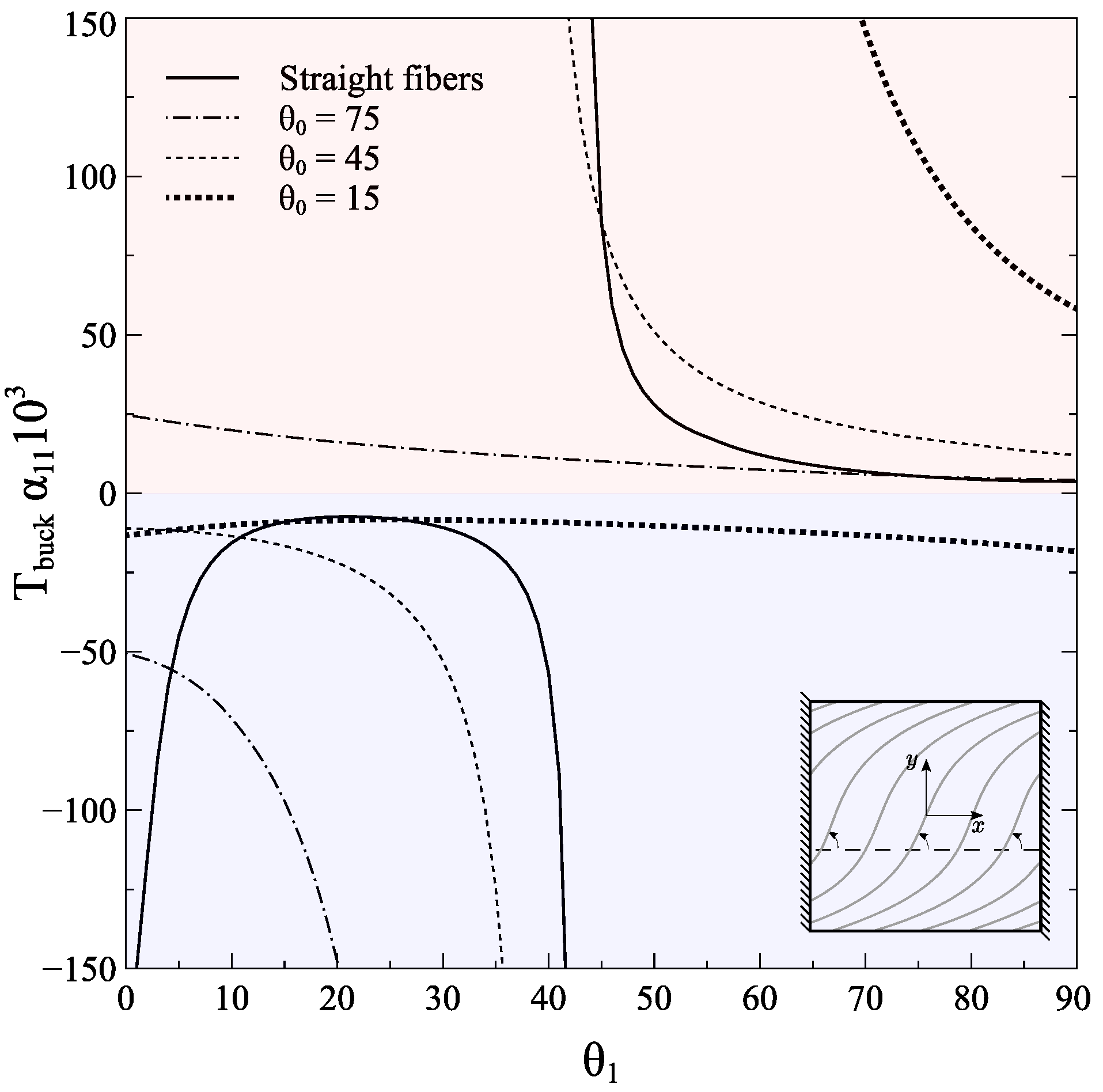
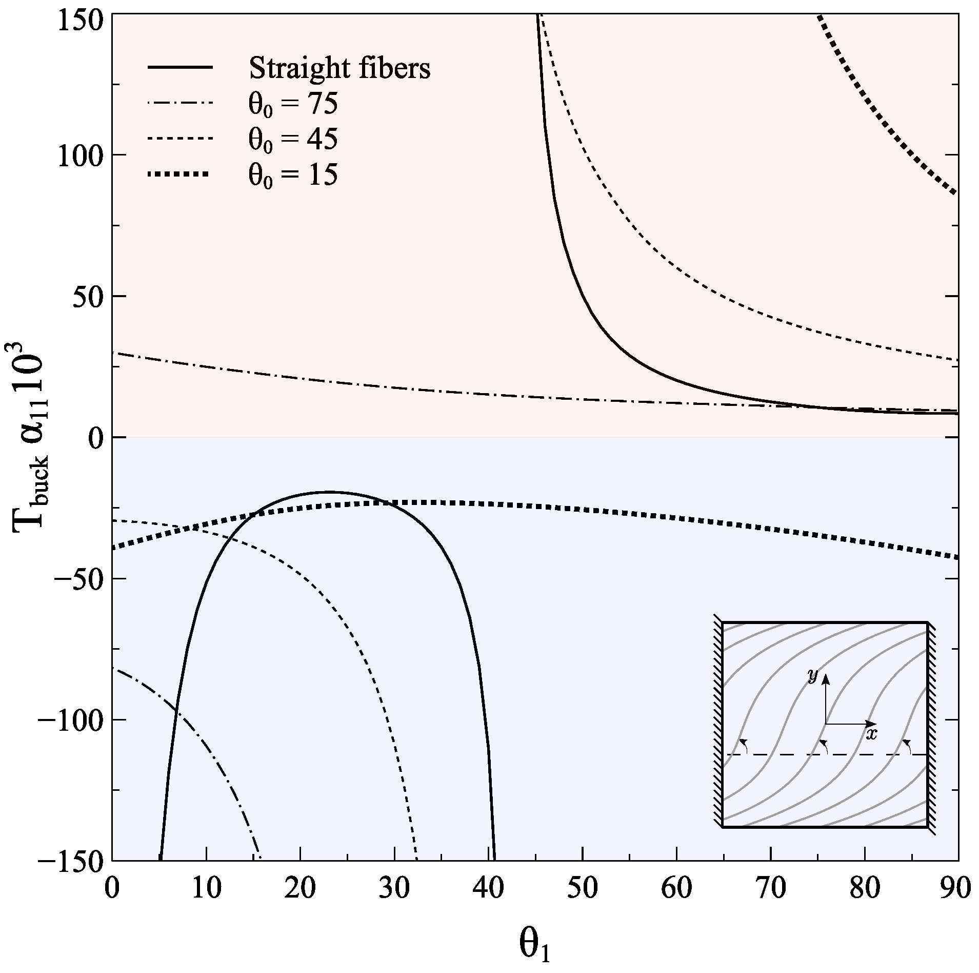
3.2. Pre-Buckling and Buckling Response of Carbon/Epoxy VSP

Having demonstrated the capabilities of the Ritz formulation, further results are discussed in this section. The present study focuses on carbon/epoxy composites, which are commonly employed in advanced constructions such as in the aerospace field. The material properties are those relative to the Graphite/Epoxy material of Table 3, and taken from [36]. For convenience, they are reported here below:

• $E_{11}$ = 155,000 MPa,
• $E_{33}$ = $E_{22}$ = 8070 MPa,
• $G_{12}$ = $G_{13}$ = $G_{23}$ = 4550 MPa,
• ${\nu }_{12}$ = ${\nu }_{13}$ = ${\nu }_{23}$ = 0.22,
• ${\alpha }_{11}$ = 1$\times {10}^{-6}$/${}^{\circ }$C,
• ${\alpha }_{22}$ = 2.0.

It can be noted that the orthotropy ratio is approximately 20; the thermal coefficient along the fiber direction is slightly negative, meaning that a shortening is experienced by the material when subjected to heating, while the value is positive along the transverse direction, i.e., the matrix expands when heated. The distribution of thermal and elastic properties influences the pre-buckling stress distribution, and, in general, can be tailored by allowing the fibers to change their orientation in the panel domain. The pre-buckling distribution of internal membrane forces, in turn, affects the buckling response of the plate. Furthermore, the overall response depends upon the boundary conditions applied to the plate, with in-plane ones having the twofold effect of influencing the pre-buckling response and buckling one. Note that, for symmetric thin laminates, in-plane boundary conditions are relevant only in terms of pre-buckling response, as the out-of-plane buckling equation is uncoupled from the in-plane ones. For thick plates, whenever the assumption of in-plane stress constitutive equation is not adequate to model the plate elastic response, an inherent coupling between in-plane and out-of-plane behaviour is recovered, and the buckling behaviour is affected by the in-plane boundary conditions as well.

A set of panels is studied below here by considering the orientation of the fibers to vary along the y-axis, and the in-plane boundary conditions Case-Ty1 and Case-Ty2. The panels are square, with dimensions equal to 150 mm, and are obtained by the stacking of four plies oriented at ${[\pm <{\theta }_0|{\theta }_1{>}_y]}_s$, where the angles are measured with respect to the x axis. To illustrate how the panel response is affected by the fiber path, the angles ${\theta }_1$ are varied between 0 and 90, while two distinct angles ${\theta }_0$ are considered, and taken equal to 15 and 75. The first case corresponds to a plate with a relatively high stiffness along the x direction, at least in the middle strips of the plate close to y=0; in the second case the central region is much weaker along the x-direction due to the almost transverse orientation of the fibers.

Firstly, the results are assessed in terms of pre-buckling behaviour; then, the buckling response is illustrated, reporting also the comparison with finite element calculations.

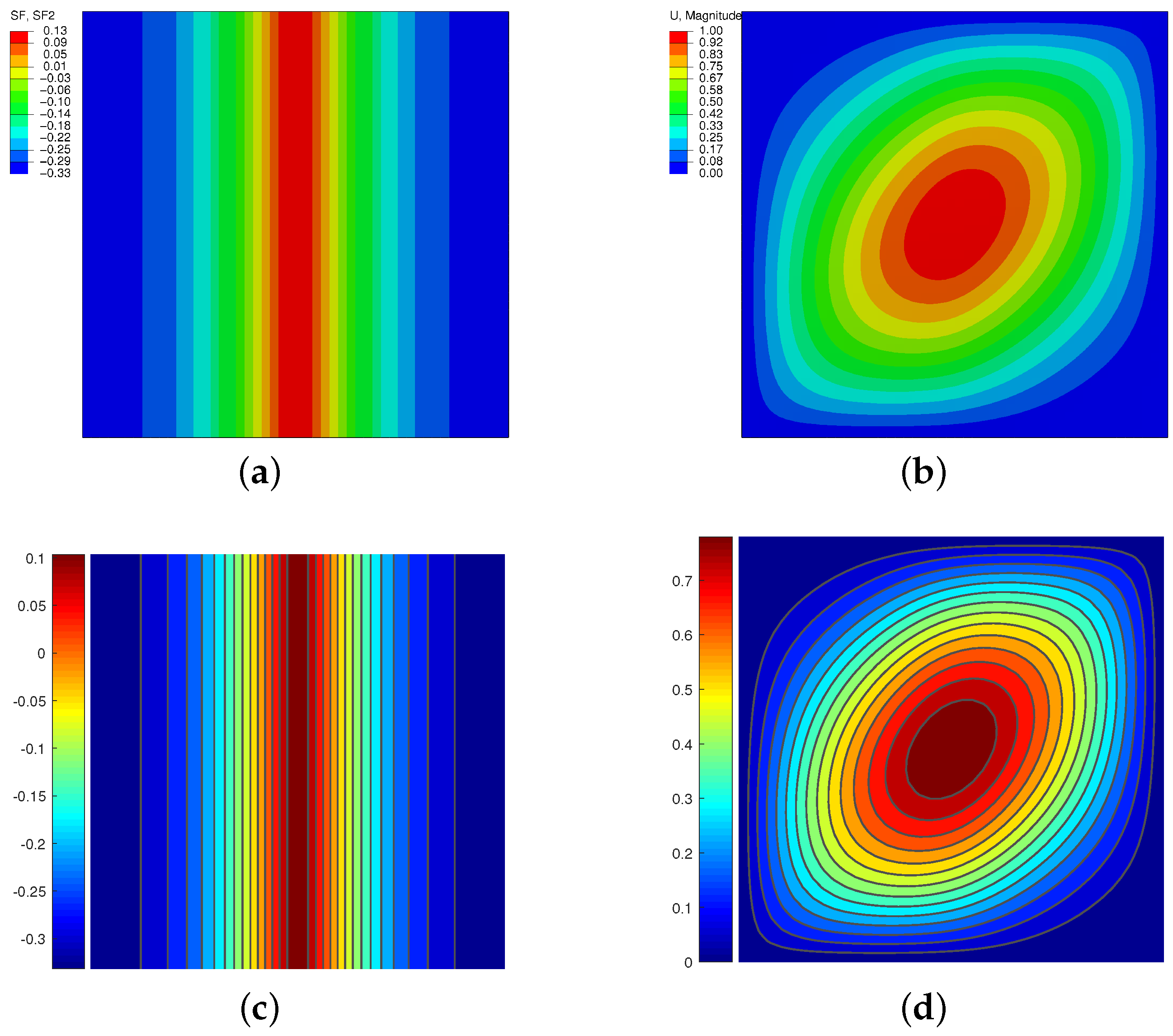
3.2.1. Pre-Buckling Analysis

Results relative to the boundary conditions Case-Ty1 are presented in Figure 6. It is recalled that the approach developed in the previous section is exact. The comparison against finite element calculations is not presented for the sake of conciseness. However, the correctness of the derivation and its implementation has been verified through an extensive set of comparisons against finite element results.

The membrane forces per unit length are calculated for a unitary temperature increase according to Equation (32), and are reported by illustrating the resultant $N_{xx}$ in the left portion of the plot, and the transverse resultant $N_{yy}$ in the right part. Positive values denote traction, while negative ones are associated with compression. Note that the curves are reported for half of the plate’s width. The remaining part can be easily recovered by exploiting the symmetry of the internal distribution with respect to the vertical axis.

Referring to Figure 6a, one can note that low values of ${\theta }_1$ are associated with fiber paths running closer to the longitudinal direction. Given the high value of the ratio $|{\alpha }_{22}/{\alpha }_{11}|$, the thermal expansion mostly relates to the transverse direction of the laminate. Due to the prescribed null displacement along the longitudinal edges, a larger force $N_y$ is introduced with respect to those cases with higher angles ${\theta }_1$. At the same time, the compressive force $N_x$ tends to increase its value for increasing orientations of the fiber angle ${\theta }_1$ at the panel’s edge. Looking, for instance, at the case with ${\theta }_1$ equal to 90, it is possible to notice the higher compressive values at the outer edge, where the thermoelastic response is dictated by the response along the matrix direction. The compressive force becomes smaller when moving towards the center of the panel, i.e., when the fibers are progressively rotated along the axial direction x.

The second case of Figure 6b is relative to a panel with fibers oriented at $\pm 75$ at the panel’s center. In this case, the steering to small values of ${\theta }_1$ (see, e.g., the case for ${\theta }_1=0$) determines a matrix-dominated response along the y-direction. The thermal dilatation is thus reacted with higher values of $N_y$. As it concerns the longitudinal direction, one can note that compressive forces are milder on the outer regions, as far as the fibers are oriented with an angle ${\theta }_1$, which is smaller than ${\theta }_0$: in these cases, the steering is such that the matrix contribution to thermal dilatation increases when moving towards the outer regions. An opposite response is observed for ${\theta }_1$ equal to 90, where the thermal dilation coefficient at the outer part is equal to that of the matrix, and larger with respect to the center, and similarly the force $N_x$.

A second set of results is available in Figure 7, where the in-plane boundary conditions Case-Ty2 are considered. The displacements along the normal direction are prevented at the transverse edges, whilst the longitudinal ones are free to expand or contract. This set of constraints is representative of a design situation where two sides of the plate are restrained with stringers characterized by high in-plane bending stiffness, such that the expansion is prevented. On the contrary, the in-plane bending stiffness of the two other parallel sides is much smaller, and the motion along the normal direction is not restrained.

From the results of Equation (36), it is seen that no membrane forces develop along the transverse direction as a response to a uniform heating or cooling. The distribution of internal forces is then purely uniaxial. The behaviour of plates characterized by ${\theta }_0$ equal to 15 is summarized in Figure 7a. One can note that steering the angle ${\theta }_1$ from 0 to 90 has the effect of increasing the laminate thermal coefficient, thus increasing the amount of compression introduced at the outer edges. For the case at hand, the smallest values of ${\theta }_1$ (0, 22.5) are characterized by a state of internal traction: thermal buckling is thus possible only if the plate is cooled. The same conclusion holds for ${\theta }_1$ equal to 45 and 67.5, as the compression region is relatively small. When ${\theta }_1$ is equal to 90, an internal state of compression is promoted, thus making the onset of instability phenomena possible due to heating.

The results of Figure 7b are relative to configurations where the fiber angle ${\theta }_0$ is equal to 75. This set of configurations is particularly interesting, as a mechanical buckling-driven design would suggest configurations where the mid angle is approximately perpendicular to the load direction in order to allow load re-distribution towards the edges. In this case, fiber angles ${\theta }_1$ equal to 90, 67.5 and 45 are associated with compressive pre-buckling force per unit length $N_x$. In other words, the matrix contribution to thermal expansion is dominant along the direction y, resulting in a compressive force in response to the prevented displacement along y at the two transverse edges. For relatively high values of fiber steering, i.e., when the external fibers are oriented at 0 or 22.5, the small thermal expansion associated with the fiber direction is such that the external parts of the plate experience a traction force resultant, whilst the inner part still is subjected to the matrix-dominated compression forces. Due to the contemporary presence of compressive and tensile internal forces, this latter configuration can undergo instability phenomena due to thermal heating.

3.2.2. Buckling Analysis

Non-dimensional buckling temperatures are reported in

Table 4. Non-dimensional thermal buckling loads $T{\alpha }_{22}\times {10}^3$ for ${[\pm <{\theta }_0|{\theta }_1{>}_y]}_s$ laminates subjected to SSSS boundary conditions. Results obtained using ED3 and 14 $\times$ 14 trial functions.

${\mathit{\theta }}_0$	${\mathit{\theta }}_1$	Case-Ty1				Case-Ty2
		$\mathit{b}/\mathit{h}$ = 100	$\mathit{b}/\mathit{h}$ = 50	$\mathit{b}/\mathit{h}$ = 20		$\mathit{b}/\mathit{h}$ = 100	$\mathit{b}/\mathit{h}$ = 50	$\mathit{b}/\mathit{h}$ = 20
15	0	0.9956	3.9413	23.0484		/	/	/
	22.5	1.4483	5.7112	32.7354		/	/	/
	45	2.0031	7.8947	44.3831		/	/	/
	67.5	1.8844	7.4340	42.8737		49.4171	173.7064	532.9265
	90	1.5486	6.1172	35.4060		15.7679	58.1094	228.6143
45	0	1.1526	4.5691	26.9298		/	/	/
	22.5	1.6750	6.6240	38.6748		879.1314	2819.5186	/
	45	2.1300	8.4043	48.6098		21.6560	85.4415	493.8370
	67.5	1.9935	7.8798	45.8766		5.4943	21.6938	125.3990
	90	1.6876	6.6841	39.1706		3.0478	12.0012	67.8208
75	0	1.0292	4.0790	24.0499		6.3514	24.7402	131.6711
	22.5	1.5674	6.1916	35.9135		3.9223	15.3611	84.2752
	45	1.9175	7.5626	43.5285		2.5716	10.0869	56.0495
	67.5	1.4448	5.6932	32.5239		1.6004	6.3060	36.0113
	90	1.0109	4.0036	23.4429		1.0726	4.2482	24.8736

for the plates discussed in the previous section. In-plane boundary conditions Case-Ty1 and Case-Ty2 are considered, while simply supported assumptions are introduced for analyzing the buckling problem.

The results are presented by considering a third-order equivalent single layer theory, ED3, while 14 trial functions are considered along both the orthogonal directions.

The results illustrate the dependence of the critical temperature with respect to the fiber path, boundary conditions and geometry of the plate. As expected, smaller values of $b/h$, i.e., thicker plates, lead to higher critical temperatures. In particular, it is noted that the pre-buckling internal forces do not depend on the panel relative thickness $b/h$, but they are a function of the thermoelastic properties only, i.e., the free thermal strains are not affected by the geometry of the plate. As a consequence, plates with different values of $b/h$, and heated with a unitary temperature increase, are subjected to the same internal resultants. On the contrary, the buckling condition depends upon the square of the ratio $h/b$, meaning that thicker plates require higher levels of internal membrane forces to buckle, and thus higher temperature increase. Based on these remarks, one can observe that the ratio between the critical temperatures associated with values of $b/h$ equal to 100 and 50 are slightly smaller than four due to effects of transverse shear flexibility. Similarly, the ratio of the temperatures of plates characterized by $b/h$ equal to 50 and 20 is slightly smaller than 6.25.

Looking at the role played by in-plane boundary conditions, it can be noted that, for a given non-dimensional parameter $b/h$, all of the critical temperatures fall in a relatively small range of value when the plate is constrained with Case-Ty1 conditions. In particular, the maximum ratio between the highest and the lowest temperatures is equal to 2, approximately. This is due to the inherent biaxiality of the internal pre-buckling forces. As noted, from the plots of Figure 6, the fiber steering has, in general, the effect of mitigating the internal compression along one direction, while increasing that on the mutually orthogonal direction, and vice versa.

A different response is observed for the in-plane conditions identified by Case-Ty2. In this case, the uniaxiality of the internal forces leads to a more pronounced dependence on the fiber path. Some configurations do not buckle under thermal heating, while they are prone to buckling as far as the fiber is steered along the transverse direction at panel edges.

For clarity, a design chart is presented in Figure 8, where the critical temperatures are reported for Case-Ty2 conditions and different stacking sequences.

The results for straight fiber configurations display, with close agreement, the behaviour illustrated by Nemeth [4]: heating-induced instability is possible in the range between $\theta$ equal to 44 and 90 degrees, while cooling is the only mechanism promoting buckling in the range between 0 and 43 degrees.

The curves of Figure 8 highlight the effect of steering the fibers. One can note that the region of instability due to heating tends to shift on the upper-right part of the plot as ${\theta }_0$ is reduced. Indeed, resistance against thermal heating is provided by longitudinally directed fibers. On the contrary, the effect of progressively rotating the center plate fibers along the longitudinal direction is that of shifting the cooling stability region to the bottom left of the plot: the matrix-dominated behaviour, at least in the central part of the plate, has the effect of improving the resistance to cooling. It is interesting to highlight that, for some range of values, buckling is possible both for heating and cooling, for temperatures that may reasonably be retained in the field of material linear response. For instance, when ${\theta }_0$ is equal to 75 and ${\theta }_1$ is 0, positive and negative critical non-dimensional temperatures are possible with absolute values of 24.74 and 50.68, respectively. The co-existence of positive and negative buckling multipliers is not possible for straight-fiber configurations, where the uniform pre-buckling condition is strictly compressive or tensile. The outlined response is thus peculiar of variable-stiffness plates, where the variability of the internal pre-buckling forces allows for the presence of non-uniform membrane force resultants with compressive and tensile regions. With similar motivations, one can observe that thermal buckling due to heating is always possible for the configurations with ${\theta }_0$ equal to 75, irrespective of the values of the fiber orientation at the edge ${\theta }_1$.

Additional results are presented in Figure 9, where the comparison is presented in terms of pre-buckling stress resultants and buckled shape for three variable-stiffness configurations with lay-up ${[\pm <{\theta }_0|90{>}_y]}_s$, and one constant stiffness panel with ${\theta }_0=90$. The internal stress distribution is evaluated referring to Equation (36) by considering a unitary temperature increase. As seen from Figure 9a–d, the internal stress non-uniformity is progressively reduced as the angle ${\theta }_0$ is increased up to 90. Note that, for clarity, the same color scale is adopted in all of the plots. With the exception of the case ${\theta }_0=15$, which is the buckling configuration associated with the plate cooling, all the other buckled surfaces are characterized by two half-waves, with increased skewness for smaller values of ${\theta }_0$ due to increased bending-twisting coupling. Despite the similarity of the buckling modes, it is noted that the critical temperatures, available from Figure 8, are drastically affected by the steering of the fibers.

The case of clamped conditions is summarized in Figure 10 to quantify the effect of flexural boundary conditions.

As expected, the effect of adding constraints is that of raising the values of critical temperatures. It can be noted that the same trends observed for the simply supported case are essentially preserved, the main difference regarding a translation of the stability regions towards higher absolute values of the temperature.

The effects of normal and transverse shear deformability are investigated in

Table 5. Non-dimensional thermal buckling loads $\frac{12}{{\pi }^2}{T}_{\mathrm{cr}}{\alpha }_{11}{\left(\frac{b}{h}\right)}^2$ for ${[\pm <{\theta }_0|{\theta }_1{>}_y]}_s$ laminates subjected to SSSS boundary conditions. Results obtained using LD2 and 14 $\times$ 14 trial functions.

${\mathit{\theta }}_0$	${\mathit{\theta }}_1$	Case-Ty1					Case-Ty2
		$\mathit{b}/\mathit{h}$ = 1000	50	20	10		$\mathit{b}/\mathit{h}$ = 1000	50	20	10
75	0	12.5529	12.3781	11.6295	9.7402		77.9289	74.9501	63.3306	39.9359
	22.5	19.1437	18.7351	17.2405	13.8214		48.0354	46.5268	40.5156	28.4722
	45	23.4373	22.8613	20.8481	15.4961		31.4840	30.5052	26.8569	19.5422
	67.5	17.6631	17.2222	15.6188	12.1018		19.5656	19.0758	17.2935	13.3857
	75	15.2747	14.9655	13.7574	10.9351		16.5691	16.2332	14.9202	11.8529
	90	12.3309	12.1678	11.3919	9.3832		13.0840	12.9108	12.0871	9.9547

by presenting the critical temperatures for different values of $b/h$. All the results are obtained referring to a layer-wise, second-order LD2 theory, which guarantees the possibility of achieving quasi-3D predictions. Aiming at highlighting the role played by higher-order deformability effects, the results are now presented according to the following non-dimensional form [4]:

$${\widehat{T}}_{\mathrm{cr}}=\frac{12}{{\pi }^2}{T}_{\mathrm{cr}}{\alpha }_{11}{\left(\frac{b}{h}\right)}^2.$$

(38)

In other words, the non-dimensional temperature is expressed in terms of the buckling coefficient ${\widehat{T}}_{\mathrm{cr}}$, which, for thin plate theory, eliminates the dependence on the geometric parameter $b/h$. In the general case of higher-order theories and for fixed plate configuration, any variation of ${\widehat{T}}_{\mathrm{cr}}$ is only ascribable to normal and transverse shear flexibility effects.

The results provide a clear insight into the importance of properly accounting for shear deformation effects, when thick and moderately thick plates of concern. For the configurations at hand, the buckling coefficients associated with $b/h$ equal to 10 are between 0.50 and 0.78 times the values registered for the thin configurations with $b/h$ equal to 1000.

It is interesting to note that the influence of the fiber orientation on transverse shear effects is relatively weak when the plate is constrained with Case-Ty1 conditions. This behaviour is ascribable to the inherent biaxiality of the internal membrane forces, which tends to reduce transverse shear deformation effects.

When the plate is constrained with Case-Ty2 conditions, the internal forces are uniaxial, and the effects of transverse shear deformability are more pronounced. Referring to Table 5, it can be noted that the relevance of transverse shear effects is higher for increasing intensities of fiber steering. The effect is at a maximum for the lay-up ${[\pm <75|10{>}_y]}_s$, where the buckling coefficient associated with $b/h$ = 10 is almost half of the one predicted for the thin plate counterpart. In those cases, the need for adopting proper kinematic theories is evident. At the same time, even the analysis of moderately thick plates in the range of $b/h$ between 50 and 20 is susceptible to noticeable approximation if thin plate theory is adopted, especially for variable-stiffness configurations with aggressive steering.

4. Conclusions

The work illustrated the analysis of the thermal buckling response of VSP using a variable-kinematics Ritz approach. The pre-buckling analysis is performed analytically and, to this aim, a set of novel closed-form solutions was derived for four different sets of in-plane boundary conditions. The availability of those solutions is particularly useful for obtaining a clear insight into the pre-buckling stress redistribution. Furthermore, it facilitates the overall buckling procedure as no linear systems need to be solved to determine the pre-buckling internal stress distributions. Due to the effectiveness of the approach, case studies can be easily conducted and design charts plotted. The results illustrate that highly accurate predictions can be achieved for thin and thick plates with uniform and variable-stiffness. The adoption of high-order theories is particularly relevant when the normal edge displacement is prevented at two parallel edges, and the two others are free to expand. Furthermore, high-steering of fibers has the effect of increasing the role played by transverse shear deformability, thus increasing even more the need for high-order theories.

References

1. Thornton, E. Thermal Structures for Aerospace Applications; AIAA: Reston, Virginia, 1996. [Google Scholar]
2. Meyers, C.; Hyer, M. Thermal buckling and postbuckling of symmetrically laminated composite plates. J. Therm. Stresses 1991, 14, 519–540. [Google Scholar] [CrossRef]
3. Jones, R. Thermal buckling of uniformly heated unidirectional and symmetric cross-ply laminated fiber-reinforced composite uniaxial in-plane restrained simply supported rectangular plates. Compos. A Appl. Sci. Manuf. 2005, 36, 1355–1367. [Google Scholar] [CrossRef]
4. Nemeth, M. Buckling behavior of long anisotropic plates subjected to restrained thermal expansion and mechanical loads. J. Therm. Stresses 2010, 23, 873–916. [Google Scholar] [CrossRef]
5. Li, J.; Narita, Y.; Wang, Z. The effects of non-uniform temperature distribution and locally distributed anisotropic properties on thermal buckling of laminated panels. Compos. Struct. 2015, 119, 610–619. [Google Scholar] [CrossRef]
6. Li, J.; Tian, X.; Han, Z.; Narita, Y. Stochastic thermal buckling analysis of laminated plates using perturbation technique. Compos. Struct. 2016, 139, 1–12. [Google Scholar] [CrossRef]
7. Tauchert, T. Thermal buckling of thick antisymmetric angle-ply laminates. J. Therm. Stresses 1987, 10, 113–124. [Google Scholar] [CrossRef]
8. Chang, J.; Shyue, S. Thermal buckling analysis of antisymmetric angle-ply laminates based on a higher-order displacement field. Compos. Sci. Technol. 1991, 41, 109–128. [Google Scholar] [CrossRef]
9. Rohwer, K. Letter to the Editor. Compos. Sci. Technol. 1992, 45, 181–182. [Google Scholar] [CrossRef]
10. Matsunaga, H. Thermal buckling of cross-ply laminated composite and sandwich plates according to a global higher-order deformation theory. Compos. Struct. 2005, 68, 439–454. [Google Scholar] [CrossRef]
11. Matsunaga, H. Thermal buckling of angle-ply laminated composite and sandwich plates according to a global higher-order deformation theory. Compos. Struct. 2006, 72, 177–192. [Google Scholar] [CrossRef]
12. Noor, A.; Burton, W. Three-dimensional solutions for thermal buckling of multilayered anisotropic plates. J. Eng. Mech. 1992, 118, 683–701. [Google Scholar] [CrossRef]
13. Noor, A.; Burton, W. Three-dimensional solutions for the thermal buckling and sensitivity derivatives of temperature-sensitive multilayered angle-ply plates. J. Appl. Mech. 1992, 59, 848–856. [Google Scholar] [CrossRef]
14. Deturk, A.; Diaz, R.; Digiovanni, G.; Hyman, B. Exploratory tests on fiber-reinforced plates with circular holes under tension. AIAA J. 1969, 7, 1820–1821. [Google Scholar] [CrossRef]
15. Leissa, A.; Martin, A. Vibration and buckling of rectangular composite plates with variable fiber spacing. Compos. Struct. 1990, 14, 339–357. [Google Scholar] [CrossRef]
16. Hyer, M.; Charette, R. Use of curvilinear fiber format in composite structure design. In Proceedings of the 30th Structures, Structural Dynamics and Material Conference, Mobile, AL, USA, 3–5 April 1989. [Google Scholar]
17. Hyer, M.; Charette, R. Use of curvilinear fiber format in composite structure design. AIAA J. 1991, 29, 1011–1015. [Google Scholar] [CrossRef]
18. Gürdal, Z.; Olmedo, R. Composite laminates with spatially varying fiber orientations: Variable stiffness panel concept. In Proceedings of the 33rd AIAA/ASME/ASCE/AHS/ASC Structures, Structural Dynamics and Material Conference, Dallas, TX, USA, 13–15 April 1992. [Google Scholar]
19. Raju, G.; Wu, Z.; Kim, B.; Weaver, P. Prebuckling and buckling analysis of variable angle tow plates with general boundary conditions. Compos. Struct. 2012, 94, 2961–2970. [Google Scholar] [CrossRef] [Green Version]
20. Wu, Z.; Weaver, P.; Raju, G.; Kim, B. Buckling analysis and optimisation of variable angle tow composite plates. Thin Walled Struct. 2012, 60, 163–172. [Google Scholar] [CrossRef] [Green Version]
21. Coburn, B.; Wu, Z.; Weaver, P. Buckling analysis of stiffened variable angle tow panels. Compos. Struct. 2014, 111, 259–270. [Google Scholar] [CrossRef] [Green Version]
22. Rahman, T.; Ijsselmuiden, S.; Abdalla, M.; Jansen, E. Postbuckling analysis of variable stiffness composite plates using a finite element-based perturbation method. Int. J. Struct. Stab. Dyn. 2011, 11, 735–753. [Google Scholar] [CrossRef]
23. Wu, Z.; Raju, G.; Weaver, P. Postbuckling analysis of variable angle tow composite plates. Int. J. Solids Struct. 2013, 50, 1770–1780. [Google Scholar] [CrossRef] [Green Version]
24. Wu, Z.; Raju, G.; Weaver, P. Framework for the buckling optimization of variable-angle tow composite plates. AIAA J. 2015, 53, 3788–3804. [Google Scholar] [CrossRef]
25. Coburn, B.; Weaver, P. Buckling analysis, design and optimisation of variable-stiffness sandwich panels. Int. J. Solids Struct. 2016, 96, 217–228. [Google Scholar] [CrossRef] [Green Version]
26. Akhavan, H.; Ribeiro, P. Natural modes of vibration of variable stiffness composite laminates with curvilinear fibers. Compos. Struct. 2011, 93, 3040–3047. [Google Scholar] [CrossRef]
27. Yazdani, S.; Ribeiro, P. A layerwise p-version finite element formulation for free vibration analysis of thick composite laminates with curvilinear fibres. Compos. Struct. 2015, 120, 531–542. [Google Scholar] [CrossRef]
28. Vescovini, R.; Dozio, L. A variable-kinematic model for variable stiffness plates: Vibration and buckling analysis. Compos. Struct. 2016, 142, 15–26. [Google Scholar] [CrossRef]
29. Carrera, E. A class of two-dimensional theories for anisotropic multilayered plates analysis. Atti Accad. Naz. Lincei Cl. Sci. Fis. Mat. Nat. Rend. 1995, 19, 1–39. [Google Scholar]
30. Carrera, E. Theories and finite elements for multilayered, anisotropic, composite plates and shells. Arch. Comput. Meth. Eng. 2002, 9, 87–140. [Google Scholar] [CrossRef]
31. Carrera, E.; Brischetto, S. A survey with numerical assessment of classical and refined theories for the analysis of sandwich plates. Appl. Mech. Rev. 2009, 62, 010803. [Google Scholar] [CrossRef]
32. Tornabene, F.; Fantuzzi, N.; Bacciocchi, M.; Viola, E. Higher-order theories for the free vibrations of doubly-curved laminated panels with curvilinear reinforcing fibers by means of a local version of the GDQ method. Compos. B Eng. 2015, 81, 196–230. [Google Scholar] [CrossRef]
33. Tornabene, F.; Fantuzzi, N.; Bacciocchi, M. Higher-order structural theories for the static analysis of doubly-curved laminated composite panels reinforced by curvilinear fibers. Thin Walled Struct. 2016, 102, 222–245. [Google Scholar] [CrossRef]
34. Tornabene, F.; Fantuzzi, N.; Bacciocchi, M. Foam core composite sandwich plates and shells with variable stiffness: Effect of the curvilinear fiber path on the modal response. J. Sandwich Struct. Mater. 2017, 1–46. [Google Scholar] [CrossRef]
35. Tornabene, F.; Bacciocchi, M. Effect of Curvilinear Reinforcing Fibers on the Linear Static Behavior of Soft-Core Sandwich Structures. J. Compos. Sci. 2018, 2, 1–41. [Google Scholar]
36. Duran, A.; Fasanella, N.; Sundararaghavan, V.; Waas, A. Thermal buckling of composite plates with spatial varying fiber orientations. Compos. Struct. 2015, 124, 228–235. [Google Scholar] [CrossRef]
37. Manickam, G.; Bharath, A.; Das, A.; Chandra, A.; Barua, P. Thermal buckling behaviour of variable stiffness laminated composite plates. Mater. Today Commun. 2018, 16, 142–151. [Google Scholar] [CrossRef]
38. Haldar, A.; Reinoso, J.; Jansen, E.; Rolfes, R. Thermally induced multistable configurations of variable stiffness composite plates: Semi-analytical and finite element investigation. Compos. Struct. 2018, 183, 161–175. [Google Scholar] [CrossRef]
39. Dano, M.L.; Hyer, M. Thermally-induced deformation behavior of unsymmetric laminates. Int. J. Solids Struct. 1998, 35, 2101–2120. [Google Scholar] [CrossRef]
40. Olmedo, R.; Gürdal, Z. Buckling response of laminates with spatially varying fiber orientations. In Proceedings of the 34th AIAA/ASME/ASCE/AHS/ASC Structures, Structural Dynamics and Material Conference, La Jolla, CA, USA, 19 April 1993–22 April 1993. [Google Scholar]
41. Waldhart, C.; Gürdal, Z.; Ribbens, C. Analysis of tow placed, parallel fiber, variable stiffness laminates. In Proceedings of the 37th AIAA Structures, Structural Dynamics, and Materials Conference, Salt Lake City, UT, USA, 15–17 April 1996. [Google Scholar] [CrossRef]
42. Carrera, E. Theories and finite elements for multilayered plates and shells: A unified compact formulation with numerical assessment and benchmarking. Arch. Comput. Meth. Eng. 2003, 10, 215–296. [Google Scholar] [CrossRef]
43. Carrera, E.; Ciuffreda, A. A unified formulation to assess theories of multilayered plates for various bending problems. Compos. Struct. 2005, 69, 271–293. [Google Scholar] [CrossRef]
44. D’Ottavio, M.; Dozio, L.; Vescovini, R.; Polit, O. Bending analysis of composite laminated and sandwich structures using sublaminate variable-kinematic Ritz models. Compos. Struct. 2016, 155, 45–62. [Google Scholar] [CrossRef]
45. Vescovini, R.; D’Ottavio, M.; Dozio, L.; Polit, O. Thermal buckling response of laminated and sandwich plates using refined 2-D models. Compos. Struct. 2017, 176, 313–328. [Google Scholar] [CrossRef]
46. Vescovini, R.; Dozio, L.; D’Ottavio, M.; Polit, O. On the application of the Ritz method to free vibration and buckling analysis of highly anisotropic plates. Compos. Struct. 2018, 192, 460–474. [Google Scholar] [CrossRef]
47. Vescovini, R.; D’Ottavio, M.; Dozio, L.; Polit, O. Buckling and wrinkling of anisotropic sandwich plates. Int. J. Eng. Sci. 2018, 130, 136–156. [Google Scholar] [CrossRef]
48. D’Ottavio, M.; Dozio, L.; Vescovini, R.; Polit, O. The Ritz–Sublaminate Generalized Unified Formulation approach for piezoelectric composite plates. Int. J. Smart Nano Mater. 2018, 9, 34–55. [Google Scholar] [CrossRef]
49. Dozio, L.; Carrera, E. Ritz analysis of vibrating rectangular and skew multilayered plates based on advanced variable-kinematic models. Compos. Struct. 2012, 94, 2118–2128. [Google Scholar] [CrossRef]
50. Gürdal, Z.; Olmedo, R. In-plane response of laminates with spatially varying fiber orientations-variable stiffness concept. AIAA J. 1993, 31, 751–758. [Google Scholar] [CrossRef]
51. Hyer, M. Stress Analysis of Fiber-Reinforced Composite Materials; McGraw-Hill: New York, NY, USA, 1998. [Google Scholar]
Figure 1. Panel geometry and reference system: (a) fiber variation along the x-direction; (b) fiber variation along the y-direction.
Jcs 02 00058 g001
Figure 2. Pre-buckling boundary conditions for fiber variation along x: (a) Case-Tx1; (b) Case-Tx2.
Jcs 02 00058 g002
Figure 3. Pre-buckling boundary conditions for fiber variation along y: (a) Case-Ty1; (b) Case-Ty2.
Jcs 02 00058 g003
Figure 4. Kevlar/Epoxy plate: (a) N y y distribution (Abaqus); (b) buckled configuration (Abaqus); (c) N y y distribution (exact; used in Ritz analysis); (d) buckled configuration (Ritz).
Jcs 02 00058 g004
Figure 5. Critical temperatures for Graphite/Epoxy, SSSS variable-stiffness plates with lay-up [ ± < θ 0 | θ 1 > x ] s . Results obtained using ED3 theory.
Jcs 02 00058 g005
Figure 6. Pre-buckling membrane resultants for [ ± < θ 0 | θ 1 > y ] s laminates subjected to Case-Ty1 conditions: (a) θ 0 = 15 ; (b) θ 0 = 75 .
Jcs 02 00058 g006
Figure 7. Pre-buckling membrane resultants for [ ± < θ 0 | θ 1 > y ] s laminates subjected to Case-Ty2 conditions: (a) θ 0 = 15 ; (b) θ 0 = 75 .
Jcs 02 00058 g007
Figure 8. Buckling design charts for different SSSS variable-stiffness configurations, b / h = 50.
Jcs 02 00058 g008
Figure 9. Pre-buckling and buckling results for SSSS variable-stiffness configurations, b/h = 50, and [ ± < θ 0 | 90 > y ] s : (a)–(d): pre-buckling distribution of internal forces Nxx, (e)–(h): buckling mode.
Jcs 02 00058 g009
Figure 10. Buckling design charts for different CCCC variable-stiffness configurations, b / h =50.
Jcs 02 00058 g010