Rheology Effects on Predicted Fiber Orientation and Elastic Properties in Large Scale Polymer Composite Additive Manufacturing


Abstract
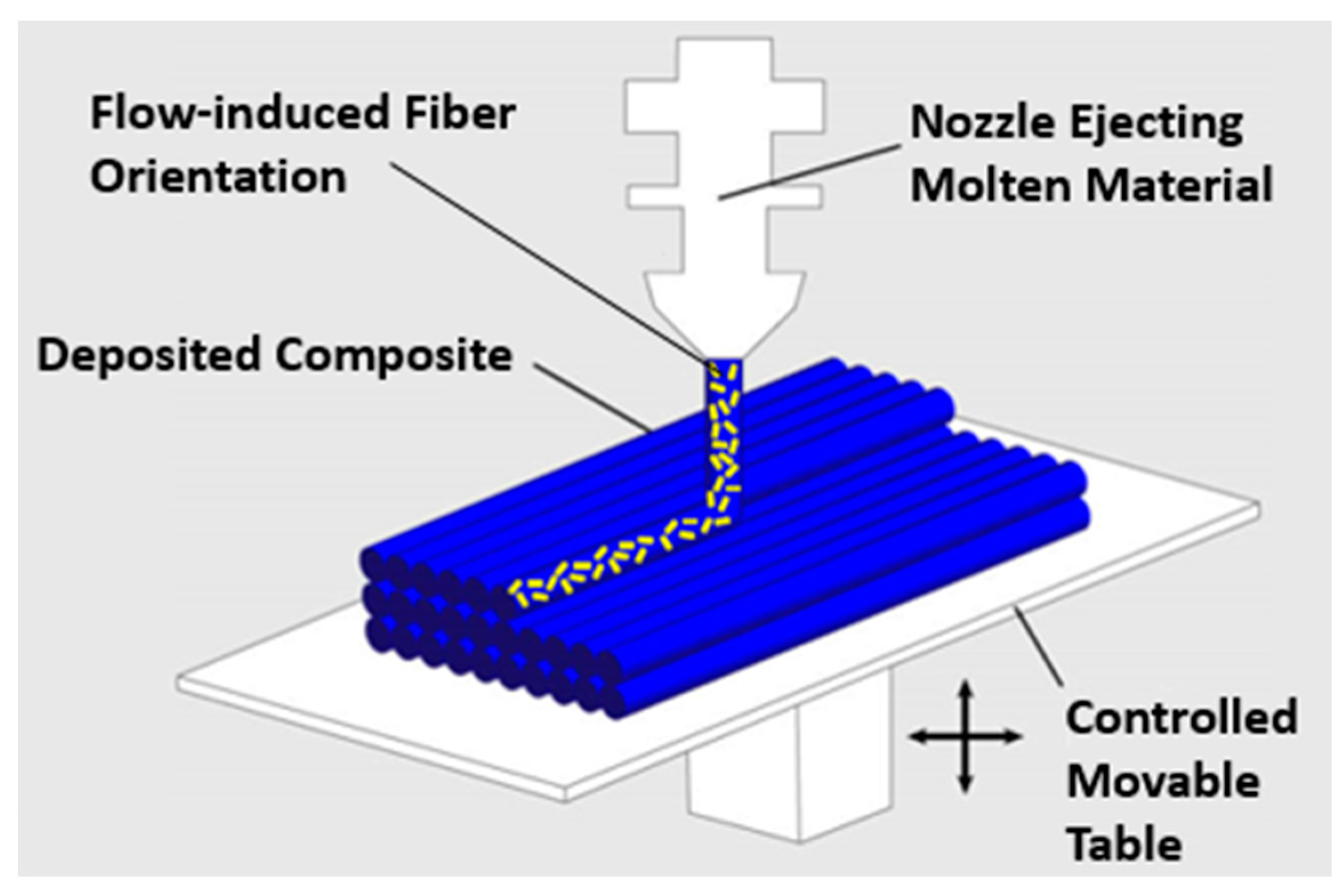
:1. Introduction
2. Materials
3. Methods
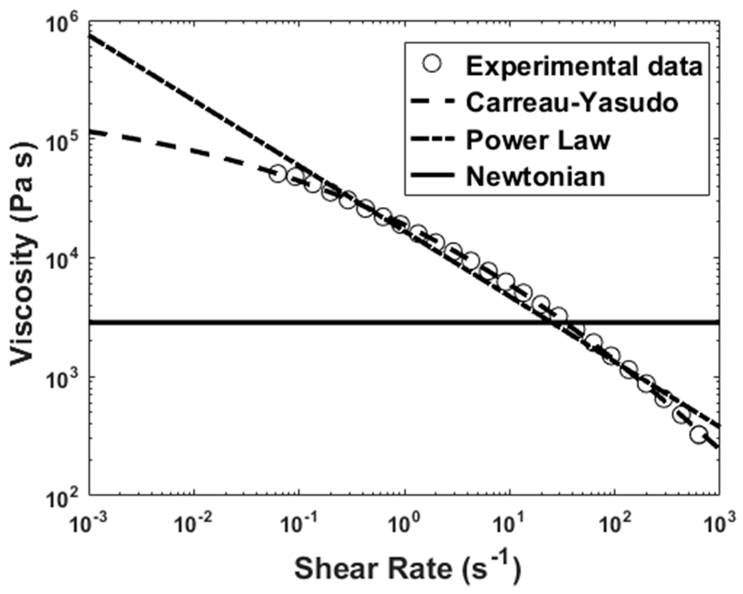
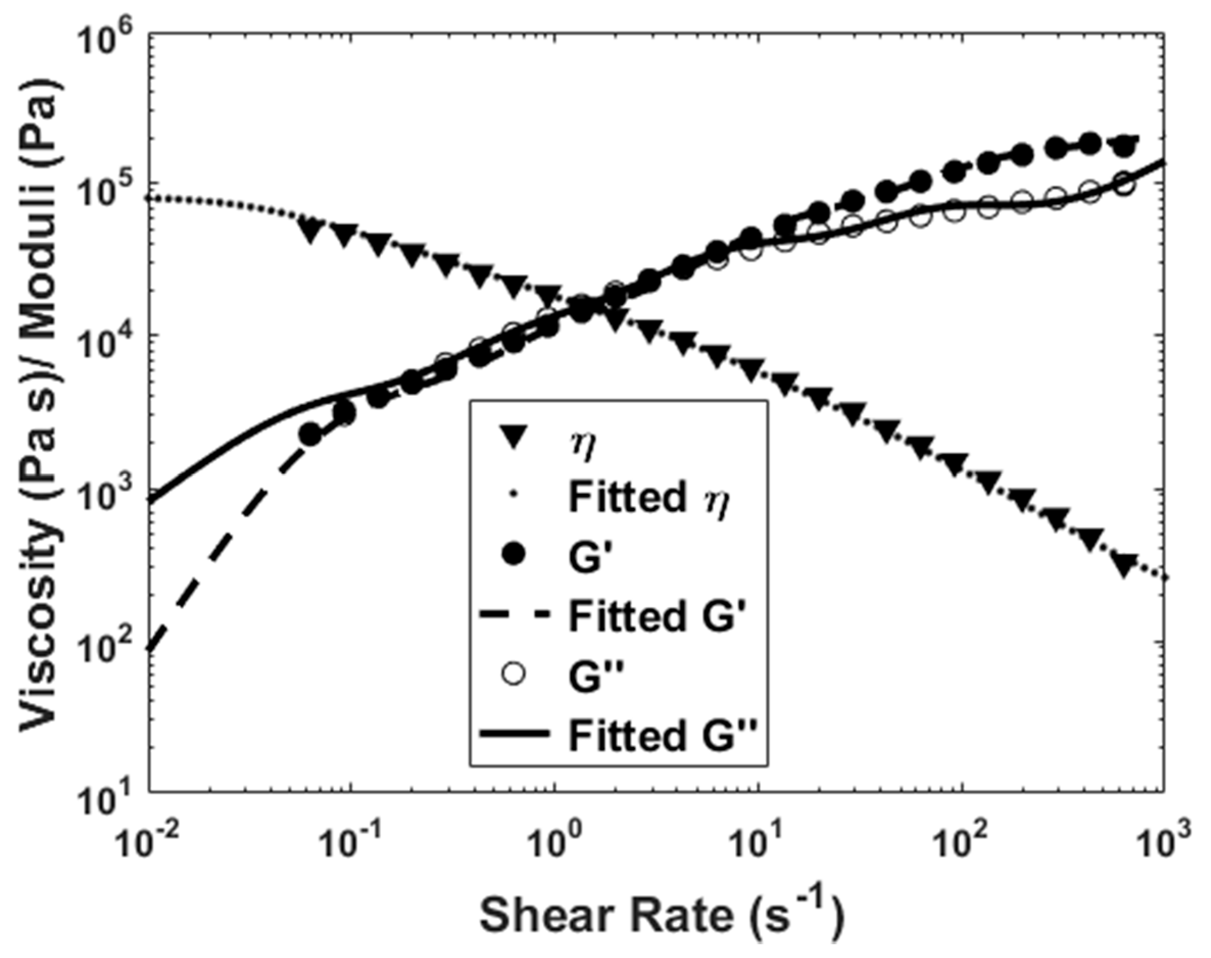
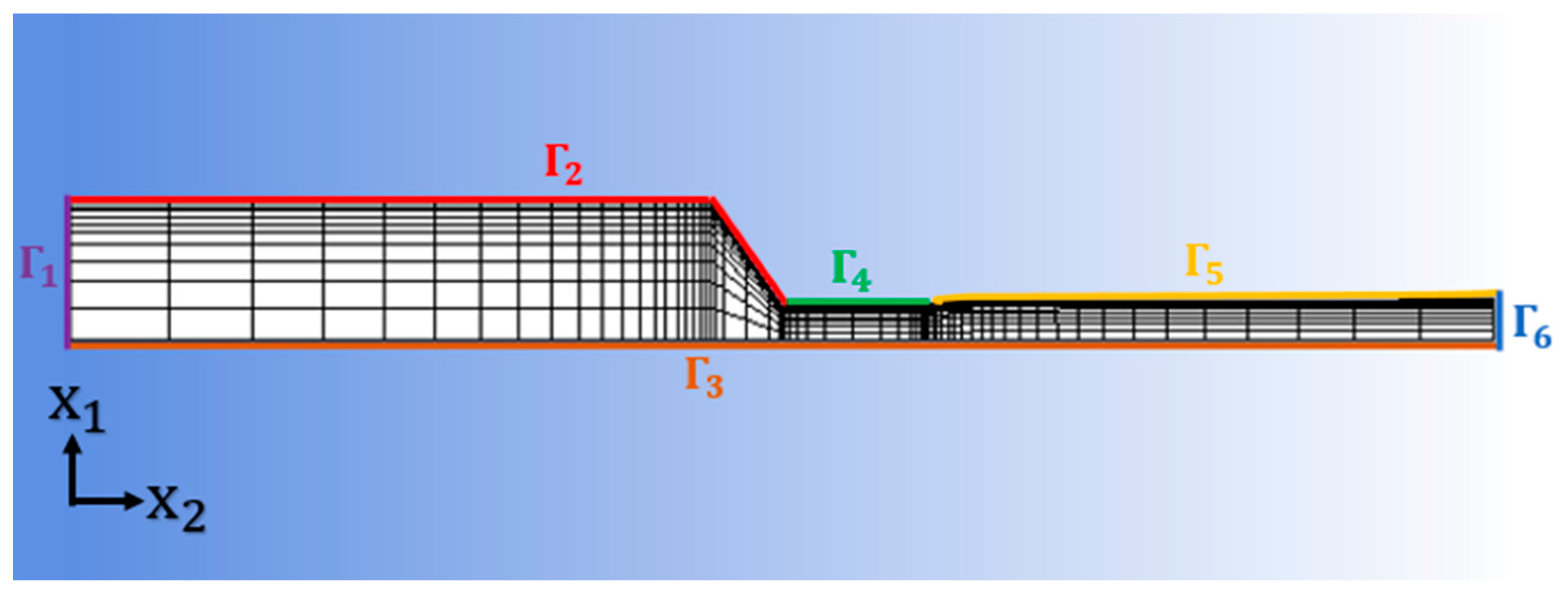
3.1. Flow Kinematics and Die Swell Evaluation
- : Flow domain inlet, where the prescribed volumetric flow rate Q is specified. In addition, a fully developed velocity profile is computed and imposed at the inlet by ANSYS-Polyflow based on Q and the selected rheology model.
- : No slip wall boundary, where .
- : Axis of symmetry, where .
- : No slip wall boundary, where .
- : Free surface, where .
- : Flow domain exit, where .
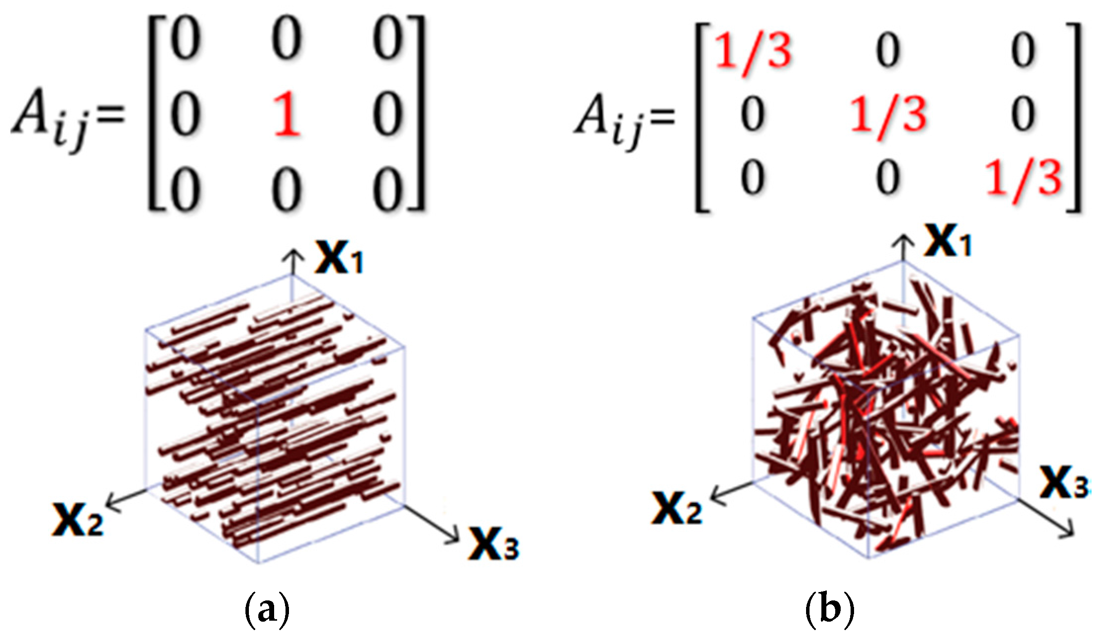
3.2. Fiber Orientation Distribution Prediction
3.3. Printed Bead Elastic Properties
4. Results and Discussions
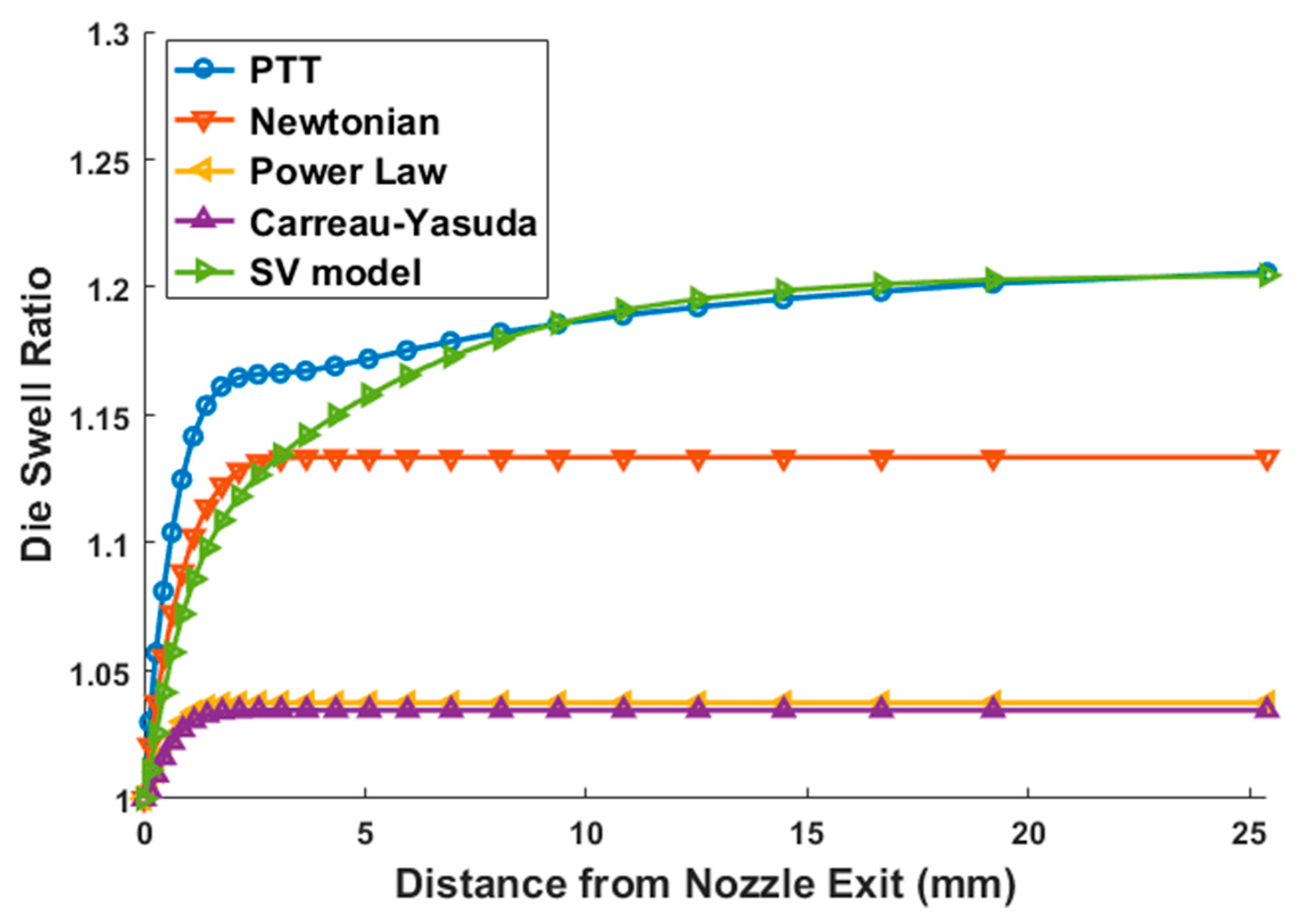
4.1. Predicted Die Swell
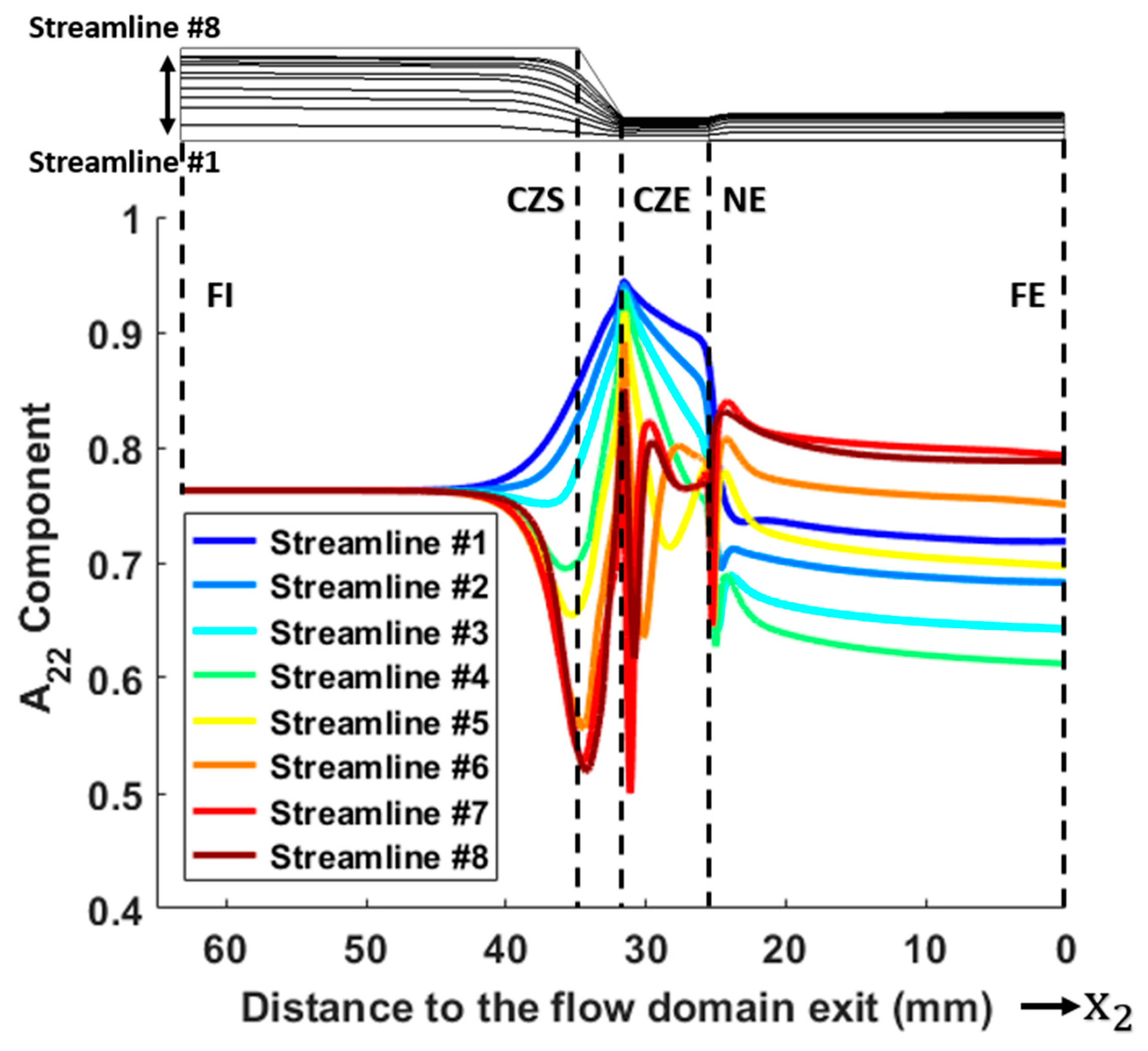
4.2. Computed Fiber Orientation Distribution
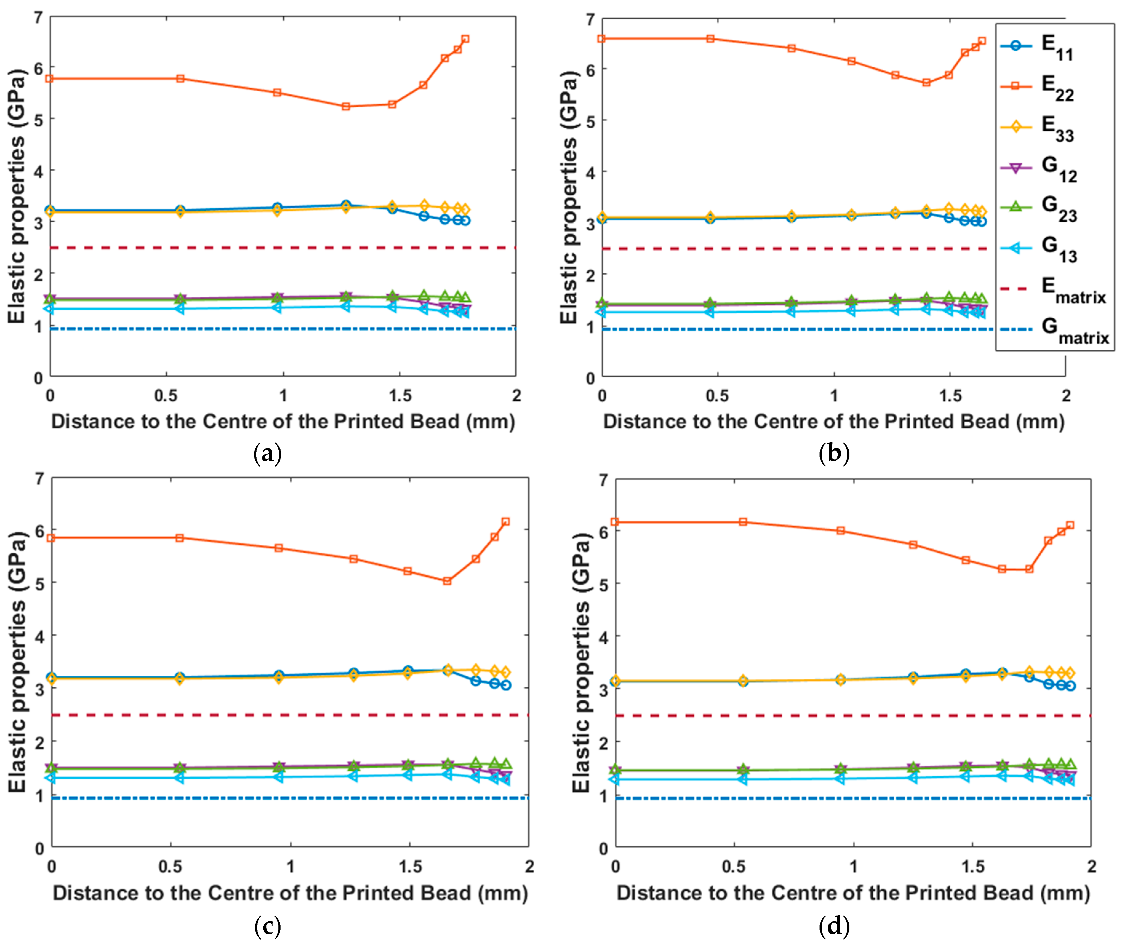
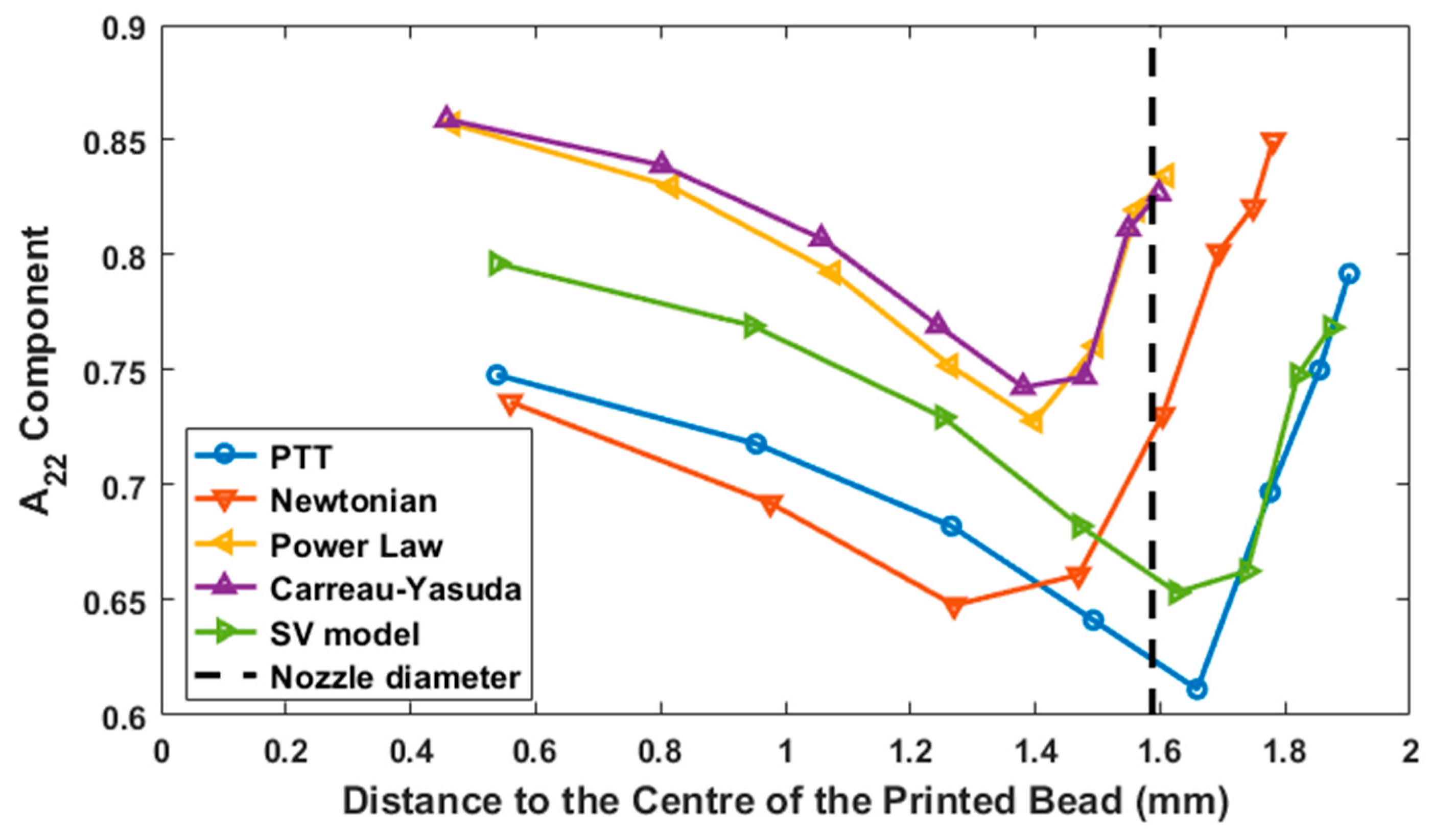
4.3. Elastic Properties across the Exrudate
5. Conclusions
Acknowledgments
Author Contributions
Conflicts of Interest
References
- Love, L.J. Utility of Big Area Additive Manufacturing (BAAM) for the Rapid Manufacture of Customized Electric Vehicles; Oak Ridge National Laboratory (ORNL); Manufacturing Demonstration Facility (MDF): Oak Ridge, TN, USA, 2015. [Google Scholar]
- Brenken, B.; Favaloro, A.; Barocio, E.; Denardo, N.; Kunc, V.; Pipes, R.B. Fused Deposition Modeling of Fiber-Reinforced Thermoplastic Polymers: Past Progress and Future Needs. In Proceedings of the American Society for Composites: Thirty-First Technical Conference, Williamsburg, VA, USA, 19–22 September 2016. [Google Scholar]
- Love, L.J.; Kunc, V.; Rios, O.; Duty, C.E.; Elliott, A.M.; Post, B.K.; Smith, R.J.; Blue, C.A. The importance of carbon fiber to polymer additive manufacturing. J. Mater. Res. 2014, 29, 1893–1898. [Google Scholar] [CrossRef]
- Duty, C.E.; Kunc, V.; Compton, B.; Post, B.; Erdman, D.; Smith, R.; Lind, R.; Lloyd, P.; Love, L. Structure and mechanical behavior of big area additive manufacturing (BAAM) materials. Rapid Prototyp. J. 2017, 23, 181–189. [Google Scholar] [CrossRef]
- Verweyst, B.E.; Tucker, C.L. Fiber suspensions in complex geometries: Flow/orientation coupling. Can. J. Chem. Eng. 2002, 80, 1093–1106. [Google Scholar] [CrossRef]
- Evans, J.G. The effect of non-Newtonian properties of a suspension of rod-like particles on flow fields. In Theoretical Rheology; Halstead Press: New York, NY, USA, 1975; pp. 224–232. [Google Scholar]
- Lipscomb, G.G.; Denn, M.M.; Hur, D.U.; Boger, D.V. The flow of fiber suspensions in complex geometries. J. Non-Newton. Fluid Mech. 1988, 26, 297–325. [Google Scholar] [CrossRef]
- Tucker, C.L. Flow regimes for fiber suspensions in narrow gaps. J. Non-Newton. Fluid Mech. 1991, 39, 239–268. [Google Scholar] [CrossRef]
- Bay, R.S.; Tucker, C.L. Fiber orientation in simple injection moldings. Part I: Theory and numerical methods. Polym. Compos. 1992, 13, 317–331. [Google Scholar] [CrossRef]
- Jackson, W.C.; Advani, S.G.; Tucker, C.L. Predicting the orientation of short fibers in thin compression moldings. J. Compos. Mater. 1986, 20, 539–557. [Google Scholar] [CrossRef]
- Nixon, J.; Dryer, B.; Lempert, I.; Bigio, D.I. Three parameter analysis of fiber orientation in fused deposition modeling geometries. In Proceedings of the PPS Conference, Cleveland, OH, USA, 8–12 June 2014. [Google Scholar]
- Phelps, J.H.; Tucker, C.L. An anisotropic rotary diffusion model for fiber orientation in short-and long-fiber thermoplastics. J. Non-Newton. Fluid Mech. 2009, 156, 165–176. [Google Scholar] [CrossRef]
- Kunc, V. Advances and challenges in large-scale polymer additive manufacturing. In Proceedings of the 15th SPE Automotive Composites Conference, Novi, MI, USA, 9–11 September 2015. [Google Scholar]
- Heller, B.; Smith, D.E.; Jack, D.A. The Effects of Extrudate Swell, Nozzle Shape, and the Nozzle Convergence Zone on Fiber Orientation in Fused Deposition Modeling Nozzle Flow. In Proceedings of the American Society of Composites—30th Technical Conference, Lansing, MI, USA, 29–30 September 2015. [Google Scholar]
- Advani, S.G.; Tucker, C.L., III. The use of tensors to describe and predict fiber orientation in short fiber composites. J. Rheol. 1987, 31, 751–784. [Google Scholar] [CrossRef]
- Crochet, M.J.; Keunings, R. Die swell of a Maxwell fluid: Numerical prediction. J. Non-Newton. Fluid Mech. 1980, 7, 199–212. [Google Scholar] [CrossRef]
- Luo, X.-L.; Tanner, R.I. A streamline element scheme for solving viscoelastic flowproblems part II: Integral constitutive models. J. Non-Newton. Fluid Mech. 1986, 22, 61–89. [Google Scholar] [CrossRef]
- Luo, X.-L.; Mitsoulis, E. An efficient algorithm for strain history tracking in finite element computations of non-Newtonian fluids with integral constitutive equations. Int. J. Numer. Methods Fluids 1990, 11, 1015–1031. [Google Scholar] [CrossRef]
- Béraudo, C.; Fortin, A.; Coupez, T.; Demay, Y.; Vergnes, B.; Agassant, J.F. A finite element method for computing the flow of multi-mode viscoelastic fluids: Comparison with experiments. J. Non-Newton. Fluid Mech. 1998, 75, 1–23. [Google Scholar] [CrossRef]
- Thien, N.P.; Tanner, R.I. A new constitutive equation derived from network theory. J. Non-Newton. Fluid Mech. 1977, 2, 353–365. [Google Scholar] [CrossRef]
- Ganvir, V.; Lele, A.; Thaokar, R.; Gautham, B.P. Prediction of extrudate swell in polymer melt extrusion using an arbitrary Lagrangian Eulerian (ALE) based finite element method. J. Non-Newton. Fluid Mech. 2009, 156, 21–28. [Google Scholar] [CrossRef]
- Limtrakarn, W.; Pratumwal, Y.; Krunate, J.; Prahsarn, C.; Phompan, W.; Sooksomsong, T.; Klinsukhon, W. Circular die swell evaluation of LDPE using simplified viscoelastic model. King Mongkut’s Univ. Technol. North Bangk. Int. J. Appl. Sci. Technol. 2013, 6, 59–68. [Google Scholar]
- Clemeur, N.; Rutgers, R.P.G.; Debbaut, B. Numerical simulation of abrupt contraction flows using the Double Convected Pom–Pom model. J. Non-Newton. Fluid Mech. 2004, 117, 193–209. [Google Scholar] [CrossRef]
- ANSYS Polyflow User’s Guide; Ansys Inc.: Canonsburg, PA, USA, 2013.
- Jack, D.A.; Smith, D.E. The effect of fibre orientation closure approximations on mechanical property predictions. Compos. Part Appl. Sci. Manuf. 2007, 38, 975–982. [Google Scholar] [CrossRef]
- Jack, D.A. Advanced Analysis of Short-Fiber Polymer Composite Material Behavior. Ph.D. Dissertation, University of Missouri, Columbia, MO, USA, 2006. [Google Scholar]
- ANSYS Polymat User’s Guide; Ansys Inc.: Canonsburg, PA, USA, 2013.
- Tadmor, Z.; Gogos, C.G. Principles of Polymer Processing; John Wiley & Sons: New York, NY, USA, 2013. [Google Scholar]
- Ajinjeru, C.; Kishore, V.; Liu, P.; Hassen, A.A.; Lindahl, J.; Kunc, V.; Duty, C. Rheological evaluation of high temperature polymer. In Proceedings of the 28th Annual International Solid Freeform Fabrication Symposium, Austin, TX, USA, 7–9 August 2017. [Google Scholar]
- Michaeli, W. Extrusion Dies for Plastics and Rubber: Design and Engineering Computations; Hanser Verlag: München, Germany, 2003. [Google Scholar]
- Reddy, J.N.; Gartling, D.K. The Finite Element Method in Heat Transfer and Fluid Dynamics; CRC Press: Boca Raton, FL, USA, 2010; Volume 32. [Google Scholar]
- Fu, S.-Y.; Yue, C.-Y.; Hu, X.; Mai, Y.-W. Characterization of fiber length distribution of short-fiber reinforced thermoplastics. J. Mater. Sci. Lett. 2001, 20, 31–33. [Google Scholar] [CrossRef]
- Verleye, V.; Couniot, A.; Dupret, F. Prediction of fiber orientation in complex injection molded parts. In Proceedings of the Ninth International Conference on Composite Materials (ICCM/9), Madrid, Spain, 12–16 July 1993; Volume 3, pp. 642–650. [Google Scholar]
- Dupret, F.; Verleye, V.; Languillier, B. Numerical prediction of the molding of composite parts. ASME-Publ.-FED 1997, 243, 79–90. [Google Scholar]
- Cintra, J.S., Jr.; Tucker, C.L., III. Orthotropic closure approximations for flow-induced fiber orientation. J. Rheol. 1995, 39, 1095–1122. [Google Scholar] [CrossRef]
- Chung, D.H.; Kwon, T.H. Improved model of orthotropic closure approximation for flow induced fiber orientation. Polym. Compos. 2001, 22, 636–649. [Google Scholar] [CrossRef]
- Meyer, K.J.; Hofmann, J.T.; Baird, D.G. Initial conditions for simulating glass fiber orientation in the filling of center-gated disks. Compos. Part Appl. Sci. Manuf. 2013, 49, 192–202. [Google Scholar] [CrossRef]
- Mase, G.T.; Smelser, R.E.; Mase, G.E. Continuum Mechanics for Engineers; CRC Press: Boca Raton, FL, USA, 2009. [Google Scholar]
- Tandon, G.P.; Weng, G.J. The effect of aspect ratio of inclusions on the elastic properties of unidirectionally aligned composites. Polym. Compos. 1984, 5, 327–333. [Google Scholar] [CrossRef]
- Reddy, K.R.; Tanner, R.I. Finite element solution of viscous jet flows with surface tension. Comput. Fluids 1978, 6, 83–91. [Google Scholar] [CrossRef]
- ANSYS CFD-Post User’s Guide; Ansys Inc.: Canonsburg, PA, USA, 2012.
- Chapra, S.C. Applied Numerical Methods with MATLAB for Engineers and Scientists; McGraw Hill Publications: New York City, NY, USA, 2012. [Google Scholar]


| Mode No. () | (s) | (Pa s) | ||
|---|---|---|---|---|
| 1 | 0.00022 | 131.7 | 0.75 | 0.18 |
| 2 | 0.0022 | 44.7 | 0.75 | 0.18 |
| 3 | 0.012 | 1180.8 | 0.75 | 0.18 |
| 4 | 0.12 | 6286.4 | 0.75 | 0.18 |
| 5 | 1.14 | 13065.7 | 0.75 | 0.18 |
| 6 | 13.82 | 61917.7 | 0.75 | 0.18 |
| Material | Young’s Modulus, E (GPa) | Shear Modulus, G (GPa) | Poisson’s Ratio, |
|---|---|---|---|
| Carbon fiber | 230 | 95.83 | 0.2 |
| ABS matrix | 2.5 | 0.93 | 0.35 |
| Model Name | Apparent Swell Ratio |
|---|---|
| Newtonian model | 1.133 |
| Power law model | 1.037 |
| Carreau–Yasuda model | 1.035 |
| PTT model | 1.199 |
| SV model | 1.197 |
| Model Name | (GPa) | (GPa) | (GPa) | (GPa) | (GPa) | (GPa) | |||
|---|---|---|---|---|---|---|---|---|---|
| PTT | 3.48 | 6.57 | 3.50 | 1.68 | 1.68 | 1.43 | 0.22 | 0.12 | 0.21 |
| Power law | 3.32 | 7.45 | 3.40 | 1.56 | 1.63 | 1.37 | 0.20 | 0.10 | 0.22 |
| Carreau-Y. | 3.31 | 7.49 | 3.40 | 1.56 | 1.62 | 1.37 | 0.20 | 0.10 | 0.22 |
| Newtonian | 3.45 | 6.66 | 3.50 | 1.65 | 1.69 | 1.42 | 0.22 | 0.12 | 0.22 |
| SV model | 3.43 | 6.86 | 3.46 | 1.64 | 1.66 | 1.41 | 0.22 | 0.11 | 0.22 |
© 2018 by the authors. Licensee MDPI, Basel, Switzerland. This article is an open access article distributed under the terms and conditions of the Creative Commons Attribution (CC BY) license (http://creativecommons.org/licenses/by/4.0/).
Share and Cite
Wang, Z.; Smith, D.E. Rheology Effects on Predicted Fiber Orientation and Elastic Properties in Large Scale Polymer Composite Additive Manufacturing. J. Compos. Sci. 2018, 2, 10. https://doi.org/10.3390/jcs2010010
Wang Z, Smith DE. Rheology Effects on Predicted Fiber Orientation and Elastic Properties in Large Scale Polymer Composite Additive Manufacturing. Journal of Composites Science. 2018; 2(1):10. https://doi.org/10.3390/jcs2010010
Chicago/Turabian StyleWang, Zhaogui, and Douglas E. Smith. 2018. "Rheology Effects on Predicted Fiber Orientation and Elastic Properties in Large Scale Polymer Composite Additive Manufacturing" Journal of Composites Science 2, no. 1: 10. https://doi.org/10.3390/jcs2010010
APA StyleWang, Z., & Smith, D. E. (2018). Rheology Effects on Predicted Fiber Orientation and Elastic Properties in Large Scale Polymer Composite Additive Manufacturing. Journal of Composites Science, 2(1), 10. https://doi.org/10.3390/jcs2010010