Author Contributions
Conceptualization, J.H. and G.F.; methodology, J.H. and Y.C.; software, J.H.; validation, J.H., G.F. and Y.C.; formal analysis, J.H.; investigation, J.H.; resources, G.F.; data curation, J.H.; writing—original draft preparation, J.H.; writing—review and editing, J.H., G.F. and Y.C.; visualisation, J.H.; supervision, G.F.; project administration, G.F.; funding acquisition, G.F. All authors have read and agreed to the published version of the manuscript.
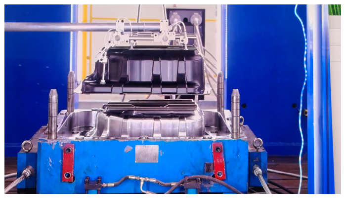
Figure 1.
Demoulding of the LFT-D PP/GF35 spare wheel well from the compression press.
Figure 1.
Demoulding of the LFT-D PP/GF35 spare wheel well from the compression press.
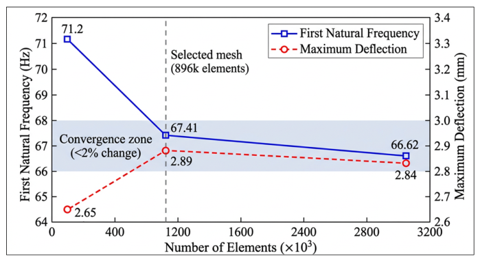
Figure 2.
Mesh convergence study showing the first natural frequency and maximum deflection under 200 N as a function of element count (five mesh densities: 48,000 to 3,024,000 elements). The 3 mm mesh (896,000 elements) was selected for production analyses, with changes of <2% between successive refinements.
Figure 2.
Mesh convergence study showing the first natural frequency and maximum deflection under 200 N as a function of element count (five mesh densities: 48,000 to 3,024,000 elements). The 3 mm mesh (896,000 elements) was selected for production analyses, with changes of <2% between successive refinements.
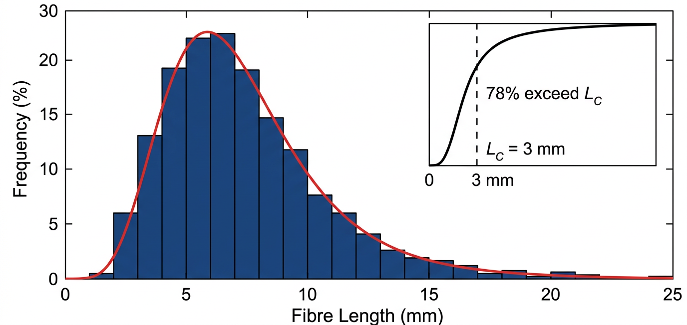
Figure 3.
Fibre length distribution histogram (n = 500). The red curve represents the fitted log-normal probability density function. Inset: cumulative distribution showing that 78% of the fibres exceed the critical length of 3 mm.
Figure 3.
Fibre length distribution histogram (n = 500). The red curve represents the fitted log-normal probability density function. Inset: cumulative distribution showing that 78% of the fibres exceed the critical length of 3 mm.
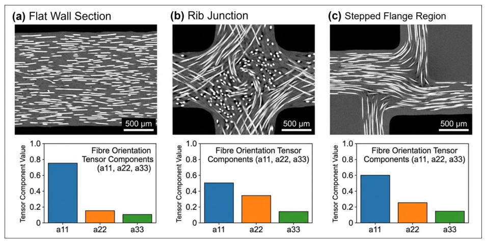
Figure 4.
Representative X-ray computed tomography (CT) cross-sections at three of nine measured locations (flat wall, rib junction, and flange) showing fibre orientation tensor components (A11, A22, A33, A12) overlaid.
Figure 4.
Representative X-ray computed tomography (CT) cross-sections at three of nine measured locations (flat wall, rib junction, and flange) showing fibre orientation tensor components (A11, A22, A33, A12) overlaid.
Figure 5.
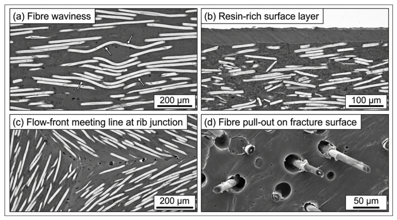
Representative micrographs of microstructural features: (a) fibre waviness at rib junction (maximum misalignment ~15°); (b) resin-rich surface layer (50–100 µm), typical of compression-moulded LFT parts; (c) flow-front meeting line at longitudinal/cross-rib junction, corresponding to elevated void content; (d) fracture surface showing limited fibre pull-out (50–150 µm), indicating good fibre–matrix adhesion.
Figure 5.
Representative micrographs of microstructural features: (a) fibre waviness at rib junction (maximum misalignment ~15°); (b) resin-rich surface layer (50–100 µm), typical of compression-moulded LFT parts; (c) flow-front meeting line at longitudinal/cross-rib junction, corresponding to elevated void content; (d) fracture surface showing limited fibre pull-out (50–150 µm), indicating good fibre–matrix adhesion.
Figure 6.
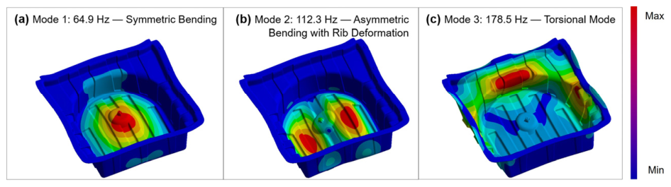
First three simulated mode shapes of the LFT-D spare wheel well: (a) Mode 1: symmetric bending of well bottom, 64.9 Hz; (b) Mode 2: asymmetric bending with rib deformation, 112.3 Hz; (c) Mode 3: torsional mode of well body, 178.5 Hz. All identified modes occur at frequencies well above the typical road excitation range (0–30 Hz).
Figure 6.
First three simulated mode shapes of the LFT-D spare wheel well: (a) Mode 1: symmetric bending of well bottom, 64.9 Hz; (b) Mode 2: asymmetric bending with rib deformation, 112.3 Hz; (c) Mode 3: torsional mode of well body, 178.5 Hz. All identified modes occur at frequencies well above the typical road excitation range (0–30 Hz).
Figure 7.
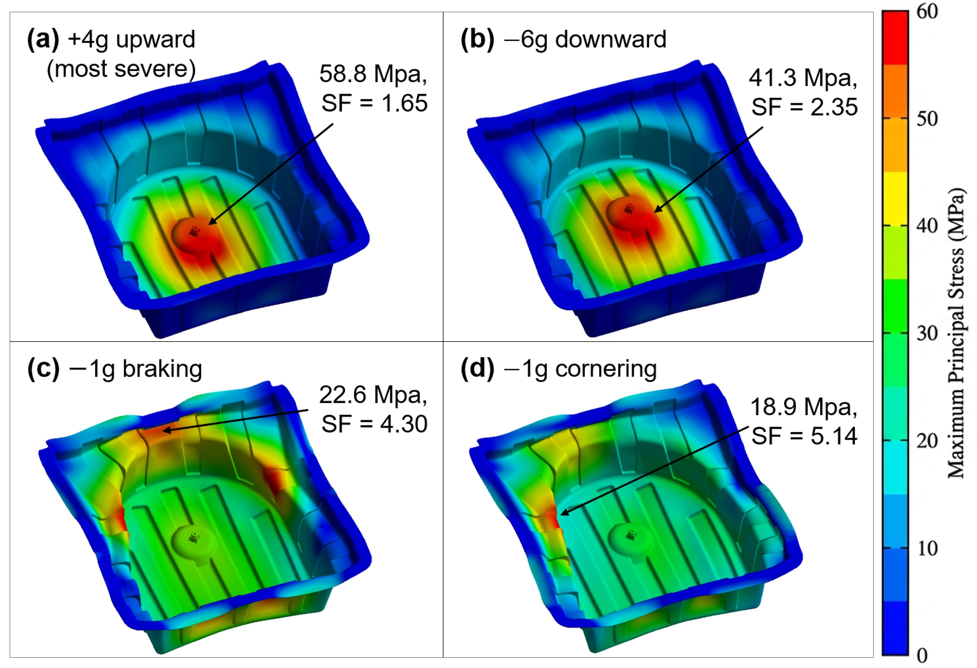
Stress distribution contour plots for all four strength load cases evaluated using the orthotropic FE model. Maximum principal stresses and corresponding safety factors are annotated. All stresses are below the material tensile strength of 97.1 MPa, with a minimum safety factor of 1.65 under the +4 g upward load.
Figure 7.
Stress distribution contour plots for all four strength load cases evaluated using the orthotropic FE model. Maximum principal stresses and corresponding safety factors are annotated. All stresses are below the material tensile strength of 97.1 MPa, with a minimum safety factor of 1.65 under the +4 g upward load.
Figure 8.
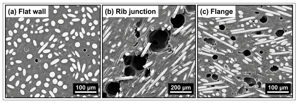
SEM images of void morphology: (a) flat wall region showing isolated micro-voids (10–40 µm); (b) rib junction cross-section showing clustered voids (20–350 µm) at the flow-front meeting line; (c) flange region showing scattered voids (20–150 µm). The higher void content at rib junctions (3.2 ± 0.8%) arises from entrapped air during fountain flow at the thickness transition, compared with 0.8 ± 0.3% at the flat wall and 1.5 ± 0.4% at the flange.
Figure 8.
SEM images of void morphology: (a) flat wall region showing isolated micro-voids (10–40 µm); (b) rib junction cross-section showing clustered voids (20–350 µm) at the flow-front meeting line; (c) flange region showing scattered voids (20–150 µm). The higher void content at rib junctions (3.2 ± 0.8%) arises from entrapped air during fountain flow at the thickness transition, compared with 0.8 ± 0.3% at the flat wall and 1.5 ± 0.4% at the flange.
Figure 9.
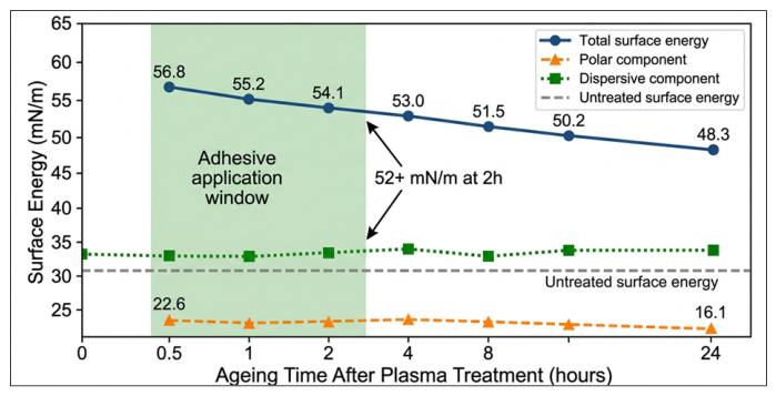
Surface energy of plasma-treated PP as a function of ageing time. Total surface energy (γ_total), dispersive component (γ_D), and polar component (γ_P) were calculated using the OWRK method. The total surface energy decreases from 56.8 mN/m to 48.3 mN/m after 24 h, indicating partial hydrophobic recovery. In production, adhesive is applied within 2 h when surface energy exceeds 52 mN/m.
Figure 9.
Surface energy of plasma-treated PP as a function of ageing time. Total surface energy (γ_total), dispersive component (γ_D), and polar component (γ_P) were calculated using the OWRK method. The total surface energy decreases from 56.8 mN/m to 48.3 mN/m after 24 h, indicating partial hydrophobic recovery. In production, adhesive is applied within 2 h when surface energy exceeds 52 mN/m.
Figure 10.
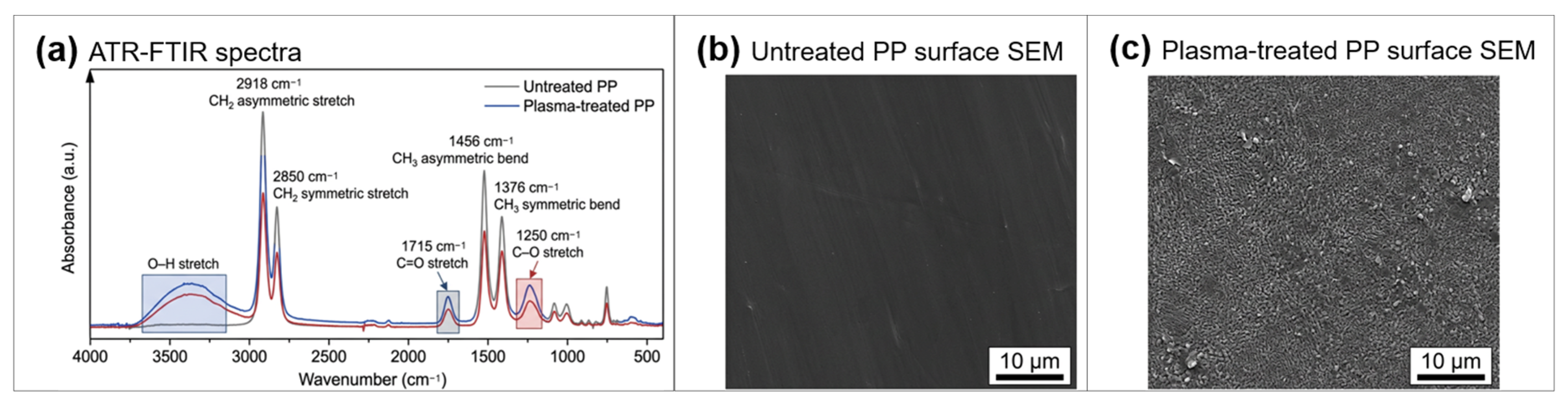
Surface characterisation of plasma-treated PP: (a) ATR-FTIR spectra of untreated PP (grey curve), plasma-treated PP (blue curve), and its smoothed spectrum (red curve) highlighting newly introduced O–H, C=O, and C–O groups (shaded boxes); (b) untreated PP surface SEM; (c) plasma-treated PP surface SEM.
Figure 10.
Surface characterisation of plasma-treated PP: (a) ATR-FTIR spectra of untreated PP (grey curve), plasma-treated PP (blue curve), and its smoothed spectrum (red curve) highlighting newly introduced O–H, C=O, and C–O groups (shaded boxes); (b) untreated PP surface SEM; (c) plasma-treated PP surface SEM.
Figure 11.
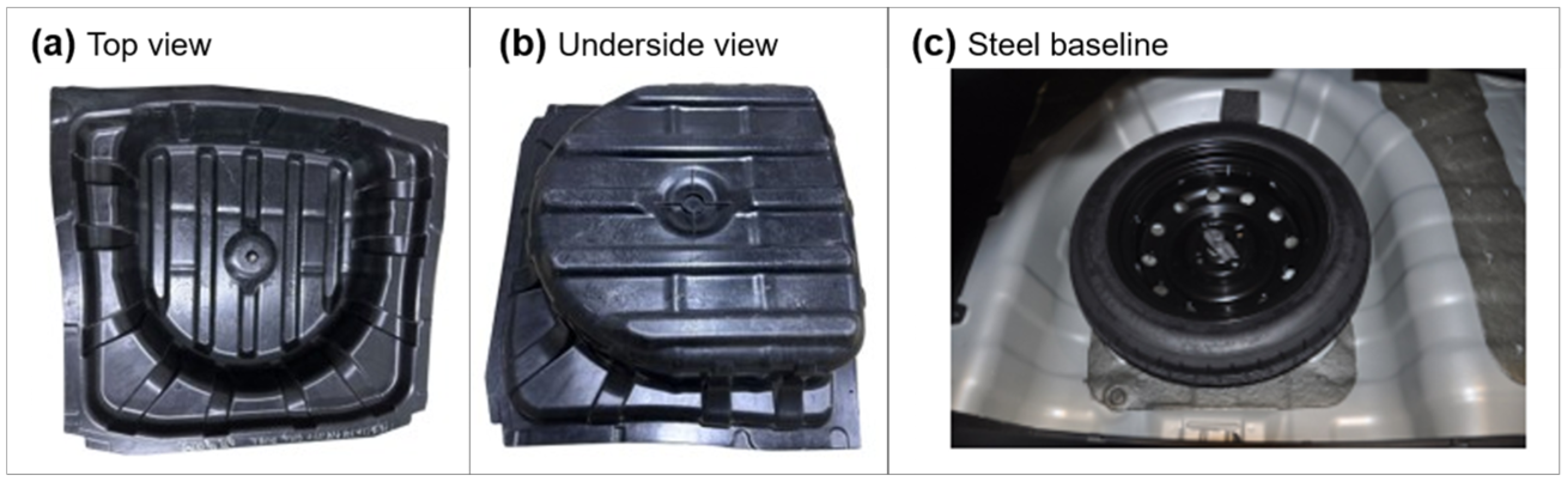
(a) Top view of the LFT-D prototype showing longitudinal ribs and central insert. (b) Underside view showing cross-shaped and radial ribs. (c) The seven-piece welded steel spare wheel well assembly.
Figure 11.
(a) Top view of the LFT-D prototype showing longitudinal ribs and central insert. (b) Underside view showing cross-shaped and radial ribs. (c) The seven-piece welded steel spare wheel well assembly.
Figure 12.
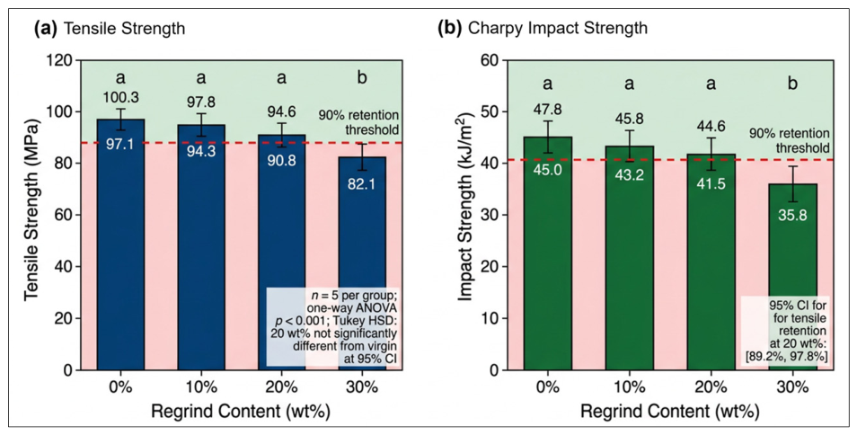
Effect of regrind content on (
a) tensile strength (MPa, blue bars) and (
b) Charpy notched impact strength (kJ/m
2, green bars) at four regrind levels (0, 10, 20, 30 wt%). Bars are means (n = 5); error bars are ± 1 standard deviation (SD). The red dashed line marks the 90% retention threshold relative to virgin material. Different letters (a/b) denote significant differences by one-way analysis of variance (ANOVA) with Tukey honestly significant difference (HSD) (
p < 0.05): 0–20 wt% (group a) are indistinguishable from virgin, while 30 wt% (group b) is significantly lower. The 95% confidence interval (CI) for tensile strength retention at 20 wt% regrind was between 89.2% and 97.8%. Numerical values are given in
Table 13.
Figure 12.
Effect of regrind content on (
a) tensile strength (MPa, blue bars) and (
b) Charpy notched impact strength (kJ/m
2, green bars) at four regrind levels (0, 10, 20, 30 wt%). Bars are means (n = 5); error bars are ± 1 standard deviation (SD). The red dashed line marks the 90% retention threshold relative to virgin material. Different letters (a/b) denote significant differences by one-way analysis of variance (ANOVA) with Tukey honestly significant difference (HSD) (
p < 0.05): 0–20 wt% (group a) are indistinguishable from virgin, while 30 wt% (group b) is significantly lower. The 95% confidence interval (CI) for tensile strength retention at 20 wt% regrind was between 89.2% and 97.8%. Numerical values are given in
Table 13.
Table 1.
Summary of LFT-D applications in automotive components.
Table 1.
Summary of LFT-D applications in automotive components.
| Technology | Material | Process | Application | Component Size (mm) | Fibre Content (wt%) | Reference |
|---|
| SMC | UP/GF (thermoset) | Compression moulding | Spare wheel well, closure panels | 1100 × 900 × 350 | 25–35 | [8,9] |
| GMT | PP/GF mat | Sheet preheat + compression | Spare wheel well | 1100 × 900 × 300 | 30–40 | [10] |
| LFT-G | PP/GF pellets | Injection/compression moulding | Small-medium semi-structural | 500 × 300 × 100 | 30–40 | [6,7] |
| LFT-D | PP/GF direct roving | In-line compounding + compression | Front-end carrier | 1200 × 400 × 150 | 30–40 | [6,16] |
| LFT-D | PP/GF direct roving | In-line compounding + compression | Battery enclosure | 1500 × 1000 × 200 | 35–45 | [6,16] |
| LFT-D | PP/GF direct roving | In-line compounding + compression | Bumper beam | 1400 × 150 × 100 | 35–45 | [6] |
| LFT-D | PP/GF direct roving | In-line compounding + compression | Spare wheel well (this work) | 1100 × 900 × 350 | 35 | Present study |
Table 2.
Key LFT-D processing parameters.
Table 2.
Key LFT-D processing parameters.
| Parameter | Value | Unit |
|---|
| Melt temperature at die | 218 ± 2 | °C |
| Screw speed | 180 | rpm |
| Barrel temperature (Zones 1–6) | 190/200/210/215/220/218 | °C |
| Fibre feed rate | 14.5 ± 0.5 | kg/h |
| Total throughput | 42.0 | kg/h |
| Average residence time | 45 ± 5 | s |
| Mould temperature (upper/lower) | 60/40 | °C |
| Compression force | 2500 | t |
| Equivalent specific pressure | 30 * | MPa |
| Holding time | 45 | s |
| Mould closing velocity | 150 | mm/s |
| Total cycle time | 58 | s |
| Charge transfer time | 3.2 ± 0.3 | s |
| Cooling time (in mould) | 45 | s |
Table 3.
Mechanical properties of the LFT-D PP/GF35 material (mean ± SD, n = 5).
Table 3.
Mechanical properties of the LFT-D PP/GF35 material (mean ± SD, n = 5).
| Property | Value | Test Standard |
|---|
| Density (g/cm3) | 1.15 ± 0.05 | ISO 1183 [20] |
| Tensile strength (MPa) | 97.1 ± 3.2 | ISO 527-2 [21] |
| Tensile modulus (GPa) | 5.82 ± 0.21 | ISO 527-2 [21] |
| Flexural strength (MPa) | 152 ± 8 | ISO 14125 [18] |
| Flexural modulus (GPa) | 5.33 ± 0.25 | ISO 14125 [18] |
| Compressive strength (MPa) | 85 ± 5 | ISO 604 [19] |
| Charpy notched impact, 23 °C (kJ/m2) | 45.0 ± 2.8 | ISO 179-1 [22] |
Table 4.
Fibre length distribution statistics (n = 500).
Table 4.
Fibre length distribution statistics (n = 500).
| Property | Value |
|---|
| Number-average length, Ln (mm) | 5.3 |
| Mass-average length, Lw (mm) | 7.2 |
| Median length (mm) | 4.6 |
| Mode (mm) | 3.4 |
| Standard deviation (mm) | 3.2 |
| Coefficient of variation (%) | 59 |
| Polydispersity index (Lw/Ln) | 1.35 |
| Minimum (mm) | 0.8 * |
| Maximum (mm) | 18.5 * |
| Skewness | 1.6 * |
| Fibres > 3 mm (critical length) (%) | 78 |
| Distribution fit | Log-normal (µ = 1.52, σ = 0.55) * |
Table 5.
Experimental test programme and acceptance criteria.
Table 5.
Experimental test programme and acceptance criteria.
| No. | Test | Standard | Acceptance Criterion | n |
|---|
| 1 | Stiffness (200 N) | Internal original equipment manufacturer (OEM) spec | Deflection ≤ 4 mm | 3 |
| 2 | Constrained modal | Internal OEM spec | First frequency ≥ 50 Hz | 3 |
| 3 | Thermal cycling (−40 to 80 °C) | ISO 16750-4 [32] | No blister or crack | 3 |
| 4 | Low-temp impact (−40 °C) | Internal OEM spec | No through-thickness crack | 3 |
| 5 | Stone impact | SAE J400 [33] | No through-thickness crack | 3 |
| 6 | Road simulation (7000 km eq.) | Internal OEM spec | No crack, no bond failure | 5 |
Table 6.
Fibre orientation tensor statistics by region (mean ± standard deviation [SD], n = 3 per region).
Table 6.
Fibre orientation tensor statistics by region (mean ± standard deviation [SD], n = 3 per region).
| Region | A11 | A22 | A33 |
|---|
| Flat wall | 0.68 ± 0.04 | 0.25 ± 0.03 | 0.07 ± 0.02 |
| Rib junction | 0.45 ± 0.06 | 0.32 ± 0.04 | 0.23 ± 0.03 |
| Flange | 0.52 ± 0.05 | 0.30 ± 0.04 | 0.18 ± 0.03 |
Table 7.
Comparison of FE predictions and experimental results.
Table 7.
Comparison of FE predictions and experimental results.
| Parameter | Isotropic FE | Orthotropic FE | Experimental (Mean ± SD, n = 3) | Target |
|---|
| Deflection at 200 N (mm) | 2.74 | 2.89 | 3.05 ± 0.12 | ≤4 |
| First natural frequency (Hz) | 69.12 | 67.41 | 64.90 ± 1.80 | ≥50 |
| Strength, min. SF (+4 g/−6 g/−1 g/−1 g) | No failure | No failure (SF = 1.65) * | No failure | No failure |
Table 8.
First three natural frequencies and mode shapes (n = 3).
Table 8.
First three natural frequencies and mode shapes (n = 3).
| Mode | Mode Shape | Experimental (Hz) | Orthotropic FE (Hz) | Error (%) |
|---|
| 1 | Symmetric bending | 64.90 ± 1.80 | 67.41 | 3.9 |
| 2 | Asymmetric bending + rib deformation | 112.3 ± 3.5 | 118.6 | 5.6 |
| 3 | Torsional | 178.5 ± 5.2 | 186.3 | 4.4 |
Table 9.
Void content by region (mean ± SD, n = 5 per region).
Table 9.
Void content by region (mean ± SD, n = 5 per region).
| Region | Void Content (%) | Void Size Range |
|---|
| Flat wall | 0.8 ± 0.3 | 10–80 µm |
| Rib junction | 3.2 ± 0.8 | 10–350 µm |
| Flange | 1.5 ± 0.4 | 10–150 µm |
Table 10.
Lap-shear strength under as-bonded and environmental exposure conditions (n = 10 per condition).
Table 10.
Lap-shear strength under as-bonded and environmental exposure conditions (n = 10 per condition).
| Condition | Strength (MPa) | Retention (%) |
|---|
| As-bonded (23 °C, 50% RH, 7 days) | 18.3 ± 1.4 | 100.0 |
| Salt spray (ISO 9227, 480 h) | 16.8 ± 1.2 | 91.8 |
| Humidity (40 °C, 95% RH, 1000 h) | 15.6 ± 1.5 | 85.2 |
| Thermal cycling (−40 to 80 °C, 10 cy.) | 15.0 ± 1.6 | 82.0 |
Table 11.
Complete component-level validation test results.
Table 11.
Complete component-level validation test results.
| No. | Test | Result | Status |
|---|
| 1 | Stiffness | 3.05 ± 0.12 mm | Pass |
| 2 | Constrained modal | 64.90 ± 1.80 Hz | Pass |
| 3 | Thermal cycling | No defects (3/3) | Pass |
| 4 | Low-temp impact | No cracks (3/3) | Pass |
| 5 | Stone impact | Superficial marks only (3/3) | Pass |
| 6 | Road simulation | No cracks or bond failure; superficial marks only; insert torque retention 87% * (5/5) | Pass |
Table 12.
Mass comparison between steel and LFT-D systems.
Table 12.
Mass comparison between steel and LFT-D systems.
| Component | Steel (kg) | LFT-D (kg) | Saving (%) | Note |
|---|
| Well body | 6.5 | 4.2 | 35.4 | — |
| Bracket & mounts * | 1.4 | 0 (integrated) | 100.0 | Moulded-in insert |
| Damping pad & coating * | 1.3 | 0 (eliminated) | 100.0 | Inherent damping |
| Total (system) | 9.2 | 4.2 | 54.3 | System-level |
Table 13.
Mechanical properties at each regrind level (mean ± SD, n = 5).
Table 13.
Mechanical properties at each regrind level (mean ± SD, n = 5).
| Regrind (wt%) | Tensile Str. (MPa) | Ret. (%) | Charpy (kJ/m2) | Ret. (%) | MFR |
|---|
| 0 (virgin) | 97.1 ± 3.2 | 100.0 | 45.0 ± 2.8 | 100.0 | 12.0 ± 0.5 |
| 10 | 94.3 ± 3.5 | 97.1 | 43.2 ± 2.6 | 96.0 | 13.8 ± 0.6 |
| 20 | 90.8 ± 3.8 | 93.5 | 41.5 ± 3.1 | 92.2 | 15.5 ± 0.7 |
| 30 | 82.1 ± 4.5 | 84.6 | 35.8 ± 3.5 | 79.6 | 18.2 ± 0.8 |
Table 14.
Cradle-to-gate LCA results by impact category.
Table 14.
Cradle-to-gate LCA results by impact category.
| Impact Category | Steel (kg CO2-eq) | LFT-D (kg CO2-eq) | Δ |
|---|
| Raw materials | 15.8 | 9.2 | −41.8% |
| Manufacturing | 4.8 | 2.6 | −45.8% |
| Transport | 1.5 | 1.0 | −33.3% |
| Total | 22.1 | 12.8 | −42.1% |
Table 15.
Preliminary cost comparison between steel and LFT-D systems (50,000 units/year).
Table 15.
Preliminary cost comparison between steel and LFT-D systems (50,000 units/year).
| Cost Element | Steel (USD) | LFT-D (USD) |
|---|
| Material | 8.20 | 6.50 |
| Processing (labour + en.) | 12.50 | 9.80 |
| Tooling amortisation | 3.20 | 4.50 |
| Scrap/rework | 1.10 | 0.80 |
| Total part cost | 25.00 | 21.60 |