
Article

Free Vibrations and Thermal Vibrations of Thick FGM Spherical Shells Triggered by Sinusoidal Temperature Field

Department of Mechanical Engineering, Hsiuping University of Science and Technology, Taichung 412406, Taiwan
J. Compos. Sci. 2026, 10(7), 360; https://doi.org/10.3390/jcs10070360
Submission received: 19 May 2026 / Revised: 21 June 2026 / Accepted: 23 June 2026 / Published: 6 July 2026
(This article belongs to the Section Composites Manufacturing and Processing)

Abstract

Studies of third-order shear-deformation theory (TSDT) and an advanced shear coefficient for thick-walled functionally graded material (FGM) spherical shells subjected to thermal vibrations triggered by sinusoidal temperature are presented. The nonlinear TSDT and linear and nonlinear shear coefficient can be converted into fully homogeneous equation algorithms under the sinusoidal form of free vibrations to obtain the fundamental natural frequency by using Newton’s numerical method. Then, the generalized differential quadrature (GDQ) method can be used to prepare dynamic discrete equations of motion triggered by sinusoidal temperature field in thick FGM spherical shells for materials SUS304 and Si3N4. The Young’s modulus expressed as a power-law function of thick FGM spherical shells is considered and subjected to applied thermal load. The response results of thermal stress and center displacement are compared for the cases of linear and nonlinear advanced shear coefficient, and simply and fully homogeneous equation algorithms, respectively. The practical insights for temperature effect considered in the calculation of stress and displacement are very clear and practical for FGM structures with geometries of spherical shells. The power-law function property of FGMs can be used under high temperature for four-sided simply supported constraints.

1. Introduction

Many kinds of applied load effects on functionally graded materials (FGMs) have been studied. Li (2023) [1] used the three-dimensional (3D) spring and rotational model of the finite element method (FEM) to study the collapse deformation and stress relaxation of brittle FGM spherical pores under impact load in manufacturing. Keibolahi et al. (2023) [2] applied the first-order shear-deformation theory (FSDT) of displacements to investigate thermally induced vibration in FGM deep spherical shells under rapid surface heating. Sorohan and Constantinescu (2023) [3] used FEM to study thick FGM spheres under internal and external pressures. Tamnar and Sayyad (2023) [4] presented the trigonometric displacements theory to study static porous FGM spherical shells. De Pascalis (2022) [5] used the finite difference method (FDM) to study the diffusion-induced stress (DIS) of FGM solid spheres under charge in lithium-ion batteries. Flis and Muc (2021) [6] used the complex hyper-geometric function analytical method to study the bending of porous FG spherical shells under uniform external pressure. Zannon et al. (2020) [7] used the third-order shear-deformation theory (TSDT) to investigate the fundamental frequencies of thick FGM spherical shells under free vibrations. Khinchi and Sharma (2019) [8] presented a review of the free vibrations of FGM spherical shells under thermal effects. Shahmohamadi and Kabir (2017) [9] used the FSDT to investigate buckling of FGM spherical shells under uniform external pressure and thermal load. Duc et al. (2017) [10] investigated the buckling and vibration of shallow FGM spherical shells with elastic foundations under uniform pressure and thermal loads.
The technical state of the art on the generalized differential quadrature (GDQ) of thick FGM shells and plates under thermal loads has been presented. The GDQ discrete equations of motion in matrix form can be obtained by converting the partial unknown continuous functions in the equations of motion into a summation of unknown discrete functions, subjected to the boundary condition used. It is advantageous for obtaining a direct computing solution with good computational accuracy and less computational time. It is a disadvantageous to prepare the GDQ discrete equations of motion in matrix form that include and depend on which boundary condition is used, e.g., if GDQ discrete equations of motion in matrix form have been used for the simply supported boundary condition, it is necessary to derive another set of GDQ discrete equations of motion in matrix form to be used for the clamp boundary condition. The GDQ numerical computation has been implemented using the high-level Lahey Fujitsu Fortran language. Hong (2023) [11] investigated GDQ results of a thick-walled FGM-plate subjected to thermal vibration by considering the TSDT model of displacements and a varied shear correction factor to obtain time-responses in center displacements and stresses of temperature dependent materials SUS304/Si3N4. The details about dynamic equation in TSDT of thick FGM-plate given in matrix expressions and GDQ method approximation have been also prepared. The GDQ approach used for advanced results of thick-walled FGM plates subjected to thermal vibration was presented by including the TSDT of displacements and advanced shear correction, which obtained the time responses of center displacements and stresses for temperature dependent materials SUS304/Si3N4. The details about the advanced nonlinear varied shear correction factor expression have been also presented for the GDQ results of a thick FGM circular cylindrical shell subjected to thermal vibration by Hong (2025) [12]. The TSDT of displacements and linear shear correction were provided to obtain time-response data of center displacement and stress of temperature dependent materials SUS304/Si3N4. The GDQ approach for a thick-walled FGM plate and FGM cylindrical shell subjected to thermal vibration has been presented with TSDT of displacements and advanced shear correction to obtain the time responses of center displacements and stresses for temperature dependent materials SUS304/Si3N4. The details about the advanced nonlinear varied shear correction factor expression, and dynamic equations have been also prepared with TSDT for thick-walled FGM plates and FGM cylindrical shells.
Hong (2021) [13] used the GDQ approach for a thick-walled FGM spherical shell subjected to sinusoidal thermal vibration of external loads. The TSDT of displacements and linear shear correction have been used to obtain the time response of center displacements and stress for temperature dependent materials SUS304/Si3N4. It is interesting at present to study the time responses of stress and displacement by using the GDQ approach and including the TSDT model of displacements and an advanced shear correction for thick FGM spherical shells under four-sided simply supported boundaries and thermal vibrations. Five parameters, given as environment temperature, nonlinear coefficient of TSDT, FGM power-law index, advanced shear correction and algorithms type of homogeneous equations on GDQ approaches for thick-walled FGM spherical shell, are provided. A broader investigation of independent literature about the numerical results of thick FGM spherical shells are listed as follows. Bagheri et al. (2024) [14] have applied the GDQ method to compute the thermal vibrations data for FGM spherical-conical shells. Kareem et al. (2024) [15] have reviewed the buckling and vibration of FGM spherical shells using analytical and numerical methods. Javani et al. (2019) [16] have presented the GDQ method to calculate the thermal vibrations data for FGM shallow spherical shells. Pang et al. (2019) [17] have provided a semi-analytical approaches to obtain free vibrations results for an FGM spherical shell. Sondhi et al. (2022) [18] have presented a generalized thermal solution for an FGM rotating hollow spherical body.

2. Material and Methods

For the geometries of spherical shells, two constituent materials are used in the thick FGM spherical shell and an arbitrary point is shown in Figure 1. This applies to a spherical shell subjected to a thermal load of temperature difference T only, with thickness h 1 of the inner layer FGM material 1 for metal property P m and metal volume fraction V m , and thickness h 2 of the outer layer FGM material 2 for ceramic property P c and ceramic volume fraction V c = 1 V m .
The FGM property P f g m is listed as follows,
P f g m = P m V m + P c V c
Equation (1) can become
P f g m = P m V m + P c ( 1 V m )
and the V c is listed as follows,
V c = ( z + h / 2 h ) R n
where the range of z is from z = h / 2 to z = h / 2 for the power-law function with a power-law index R n . For example, if P m = E 1 and P c = E 2 are used in the constituent Young’s modulus, then the FGM Young’s modulus E f g m can be obtained as follows. The mean expression is used for the other material properties of the FGM, e.g., Poisson’s ratio ν f g m = ν 1 + ν 2 2 , mass density ρ f g m = ρ 1 + ρ 2 2 , etc.
E f g m = ( E 2 E 1 ) ( z + h / 2 h ) R n + E 1
And the parameter L is the FGM shell’s length in the x-axial direction. A black point in the coordinates ( r ,   θ ,   ) corresponds to ( x ,   y ,   z ) , where r denotes radius of FGM shells, θ denotes circumferential-angle, and denotes angle between z and r axes. The constituent material properties of the FGM shells are a function of the environmental temperature T and are provided by Hong (2023) [11]. The equations and physical interpretations used in mathematical derivations for the approach methods are listed basically in the following subsections.

2.1. Displacements

The time vibration form of nonlinear vs. z3 in TSDT displacement components u , v , w of thick-walled FGM spherical shell are used in the following by Hong (2021) [13],
u = u 0 x , θ , t + z ϕ x x , θ , t c 1 z 3 ( ϕ x + w x ) ,
v = v 0 x , θ , t + z ϕ θ x , θ , t c 1 z 3 ( ϕ θ + w R θ ) ,
w = w x , θ , t ,
where u 0 and v 0 denote tangential displacements. w denotes transverse displacement. ϕ x and ϕ θ denote shear rotations. R denotes middle-surface radius. t is time and x = r sin cos θ . Coefficient of c 1 = 4 / [ 3 ( h ) 2 ] , where h denotes total thickness.
It is reasonable to assume that u 0 , v 0 , w , ϕ x and ϕ θ are expressed in time-sinusoidal form as follows for free vibrations without external loads with no temperature difference T = 0 , and for a shell subjected to a four-sided simply supported boundary to meet constraints at x = 0, L, and θ = 0 , 2 π , respectively,
u 0 = a m n c o s ( m π x / L ) s i n ( n π θ / R ) s i n ( ω m n t ) ,
v 0 = b m n s i n ( m π x / L ) c o s ( n π θ / R ) s i n ( ω m n t ) ,
w = c m n s i n ( m π x / L ) s i n ( n π θ / R ) s i n ( ω m n t ) ,
ϕ x = d m n c o s ( m π x / L ) s i n ( n π θ / R ) s i n ( ω m n t ) ,
ϕ θ = e m n s i n ( m π x / L ) c o s ( n π θ / R ) s i n ( ω m n t ) ,
where ω m n is the natural frequency which is operated by subscripts m and n mode shapes. The ω m n values can be obtained from the full algorithms without external loads. m is the number of axial half-waves, n is the number of circumferential waves, and a m n , b m n , c m n , d m n and e m n are the amplitudes of the time-sinusoidal form. Assumptions (8)–(12) for u 0 ,   v 0 ,   w ,   ϕ x and ϕ θ under boundaries shall satisfy no displacements and no bending moments with boundary constraints at x = 0, L, and θ = 0 , 2 π , respectively, as follows,
at   x = 0   and   x = L :   u 0 x = v 0 = w = ϕ x x = ϕ θ = 0 ,
at   θ = 0 and   θ = 2 π :   u 0 = v 0 θ = w = ϕ x = ϕ θ θ = 0 .

2.2. Full Algorithms for ω m n

By substituting Equations (8)–(12) into dynamic Equation (A1), which is listed in Appendix A, without external loads for the approach of free vibration, the full algorithms are provided in the following,
F C 11 F C 12 F C 13       F C 14 F C 15 F C 21 F C 22 F C 23       F C 24 F C 25 F C 31 F C 32 F C 33       F C 34 F C 35 F C 41 F C 42 F C 43       F C 44 F C 45 F C 51 F C 52 F C 53       F C 54 F C 55 a m n b m n c m n d m n e m n = 0 0 0 0 0 ,
in which [ F C m n ] with subscripts m, n = 1,2,…,5, are element parameters, e.g.,
F C 11 = F H 11 I 0 λ m n I 0 ,
F C 12 = F H 12 ,
F C 13 = F H 13 + c 1 I 3 m π L λ m n I 0 ,
λ m n = I 0 ω m n 2 .
And the detailed F C m n of (A10)–(A31) are listed in Appendix A.
These elements of [ F C m n ] are in functions of c 1 , I i , J i , and K 2 listed as follows,
I i = k = 1 N * k k + 1 ρ ( k ) z i d z , ( i = 0 , 1 , 2 , , 6 ) ,
J i = I i c 1 I i + 2 , ( i = 1 , 4 ) ,
K 2 = I 2 2 c 1 I 4 + c 1 2 I 6 ,
where N denotes the total layer number. ρ ( k ) is the superscript (k)th ply density, and F H m n with subscripts m, n = 1,2,…,5, are element parameters, e.g.,
F H 11 = A 11 ( m π / L ) 2 + A 66 ( n π / R ) 2 ,
F H 12 = ( A 12 + A 66 ) ( m π / L ) ( n π / R ) .
And the detailed F H m n of (A32)–(A44) are listed in Appendix A.
The ω m n can be solved from the determinant expression listed as follows, and using the usual Newton’s numerical method to solve it.
det   [ F C m n ] = 0
Also the integrals of stiffness Q ¯ i s j s and Q ¯ i j with subscripts i s , j s = 1,2,6 and i , j = 4,5 can be used as follows by Hong (2021) [13],
A i s j s , B i s j s , D i s j s , E i s j s , F i s j s , H i s j s = h 2 h 2 Q ¯ i s j s 1 , z , z 2 , z 3 , z 4 , z 6 d z ,
A i j , B i j , D i j , E i j , F i j , H i j = h 2 h 2 k α Q ¯ i j 1 , z , z 2 , z 3 , z 4 , z 5 d z ,
where k α denotes advanced nonlinear shear correction.

2.3. Stresses

The sinusoidal thermal vibrations forms of the normal stresses σ x , σ θ and shear-stresses σ x θ , σ θ z , σ x z for a thick-walled FGM spherical shell subjected to an applied thermal load with a temperature difference T from (A9) in linear vs. z on the (k)th layer, are used as follows,
σ x σ θ σ x θ σ θ z σ x z k = Q ¯ 11 Q ¯ 12 Q ¯ 16 0 0 Q ¯ 12 Q ¯ 22 Q ¯ 26 0 0 Q ¯ 16 Q ¯ 26 Q ¯ 66 0 0 0 0 0 Q ¯ 44 Q ¯ 45 0 0 0 Q ¯ 45 Q ¯ 55 k ε x α x z h T ¯ 1 sin π x L sin π θ sin γ t ε θ α θ z h T ¯ 1 sin π x L sin π θ sin γ t ε x θ α x θ z h T ¯ 1 sin π x L sin π θ sin γ t ε θ z ε x z k ,
where α x and α θ are thermal expansion coefficients. α x θ is thermal shear coefficient. ε x , ε θ and ε x θ denote in-plane strains. ε θ z and ε x z denote shear strains that are not negligible. γ is the frequency of the applied heat flux. T ¯ 1 denotes applied temperature-amplitude. The equation of heat conduction can be applied for T and the heat flux frequency equation for the γ value can be obtained by using the usual bisection iterative numerical method. In this preliminary thermal vibrations study, the author only considers the linear temperature rise vs. z in the thermo-elastic stress–strain relations. It would be more complicated and interesting to take the nonlinear temperature rise vs. functions of z2 or z3, for example, into account in future research.

2.4. Dynamic Equations of Motion by Using GDQ Discrete Approach

The dynamic equations of motion obtained by using the GDQ discrete approach can be provided in matrix form with the TSDT of FGM spherical shells, which are used and solved as follows,
[ A ] { W * } = { B }
where { W } is listed as follows,
{ W } = { U 2 , 2 , , U N 1 , M 1 , V 2 , 2 , ,   V N 1 , M 1 , W 2 , 2 , ,   W N 1 , M 1 , ϕ x 2 , 2 , ,   ϕ x N 1 , M 1 , ϕ θ 2 , 2 , ,   ϕ θ N 1 , M 1 } t ,
in which U , V , and W are listed in non-dimensional forms as follows,
U = u 0 / L ,
V = v 0 / R ,
W = w / h * ,
where N and M are grid points. [ A ] is an N by N order matrix, whose elements contain stiffness integrals, inertial terms and GDQ weighting parameters, in which N is listed as follows,
N = N 2 × ( M 2 ) × 5
{ B } denotes N th order external loads.

3. Numerical Results

Lahey Fujitsu Fortran was programmed and used to solve equations for numerical computation. The inner position material 1 of the FGMs is SUS304 and the outer position material 2 of the FGMs is Si3N4, which are provided in the numerical GDQ approach with L / R = 1 , h = 1.2 mm, and h 1 = h 2 = 0.6 mm under thermal sinusoidal vibration. The expression for individual properties, demonstrated by P i , e.g., P i = P m , for material SUS304 and P i = P c for material Si3N4 can be listed in the following
P i = P 0 ( P 1 T 1 + 1 + P 1 T + P 2 T 2 + P 3 T 3 ) ,
in which P 0 , P 1 , P 1 ,   P 2 , and P 3 denote the temperature coefficients. The values of Young’s modulus E 1 , E 2 , Poisson’s ratio ν 1 , ν 2 , mass density ρ 1 , ρ 2 , expansion coefficient α 1 , α 2 , thermal conductivity κ 1 , κ 2 and specific heat C v 1 , C v 2 for SUS304 and for Si3N4, respectively, depended on T as shown in Table 1. These parameters are used in calculation and the values of mechanical properties for the FGM bi-material thick shell can be obtained.
In this numerical study, the small spherical metal and ceramic FGM particles of the thick elastic shell provide a high Young’s modulus and very low value of natural frequency ω 11 , which is triggered by an applied sinusoidal temperature field and activated with a high value of vibration frequency γ in Equation (28). The ω 11 of the FGM is kept at an initial value, while the γ of the applied heat can take various values, e.g., from a lower frequency γ = 0.523599 rad/s and a low value γ = 15.707960 rad/s, to a high value γ = 785.3982 rad/s and super value γ = 284,314.1 rad/s, which are used for the possible frequency lower bound or the frequency range in the transient response of thermal vibration studies. The criterion used for thick shell can be considered with the ratio of the minor radius of curvature of the median curvilinear surface to the thickness which is less than 10. Typical vibration frequency ω 11 vs. c 1 , T and the power-law function in index R n for L / h = 5 at = 10 ° under both the simple algorithms and full algorithms, respectively, are shown in Table 2. These ω 11 values provided in approach of full algorithms are different from the values obtained from the simply homogeneous equation algorithms (simple algorithms, for short). The discussion of practical insights for vibration natural frequency of displacements is very important to avoid the resonance to use the same value with another rotational device. The physical meaning of the ω 11 numbers is the fundamental natural frequency coming from the displacement vibration frequency, the value of which can be affected by c 1 ,   T ,   R n and the algorithm type. The lower ω 11 numbers in the full algorithms can be found to be smaller than those in the simple algorithms.

3.1. Dynamic Convergence

The advanced dynamic convergence on displacement amplitude w ( L / 2 , 2 π / 2 ) (mm) is presented for the thermal sinusoidal vibration of nonlinear TSDT and linear studies under both c 1 = 0.925925/mm2 and c 1 = 0/mm2. The w ( L / 2 , 2 π / 2 ) values at t = 6 s for a thick FGM spherical shell at = 10 ° and L / h = 5 with γ = 0.261805 rad/s, T = 100 K, and T ¯ 1 = 100 K are presented in Table 3. The w ( L / 2 , 2 π / 2 ) data are provided on advanced values of k α , based on the free vibration ω 11 of full algorithms and in values of R n = 0.5, 1 and 2. Error data of 9.2 × 10⁻⁵ in accuracy is obtained on w ( L / 2 , 2 π / 2 ) amplitude in c 1 = 0.925925/mm2,   R n = 0.5, and L / h = 10 cases. Grid points of N × M = 13 × 13 are located for the steady state and applied to the numerical calculations. The discussion of practical insights on the convergence study in displacements is necessary for grid points which is used to make the correct and precise computation in data. The physical meaning of the w ( L / 2 , 2 π / 2 ) convergence study vs. grid points N × M at a steady state e.g., t = 6 s, is to see which grid point used is large enough to get a converged displacement and to use that grid point set subsequently for all analysis.

3.2. Time Responses

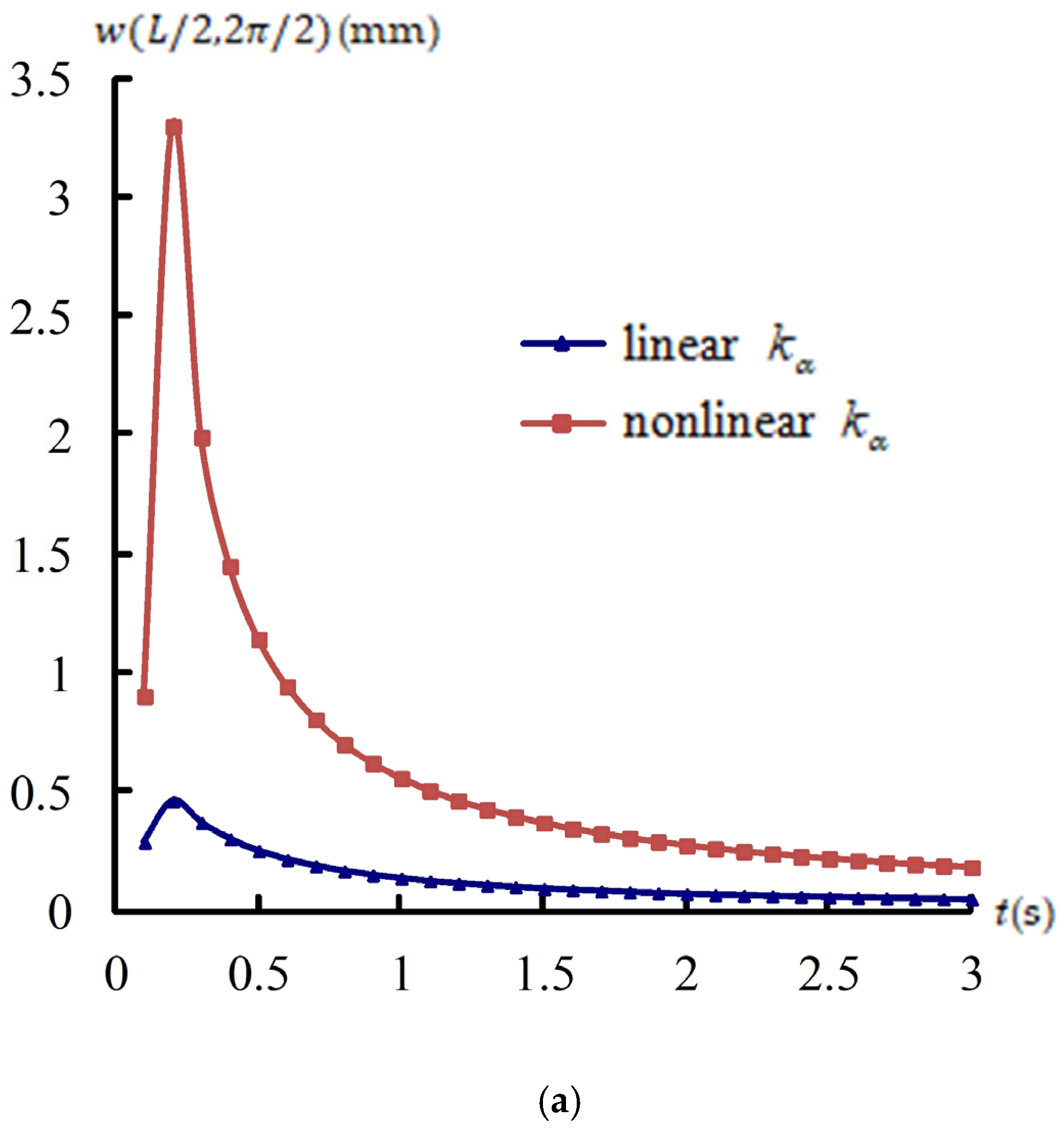
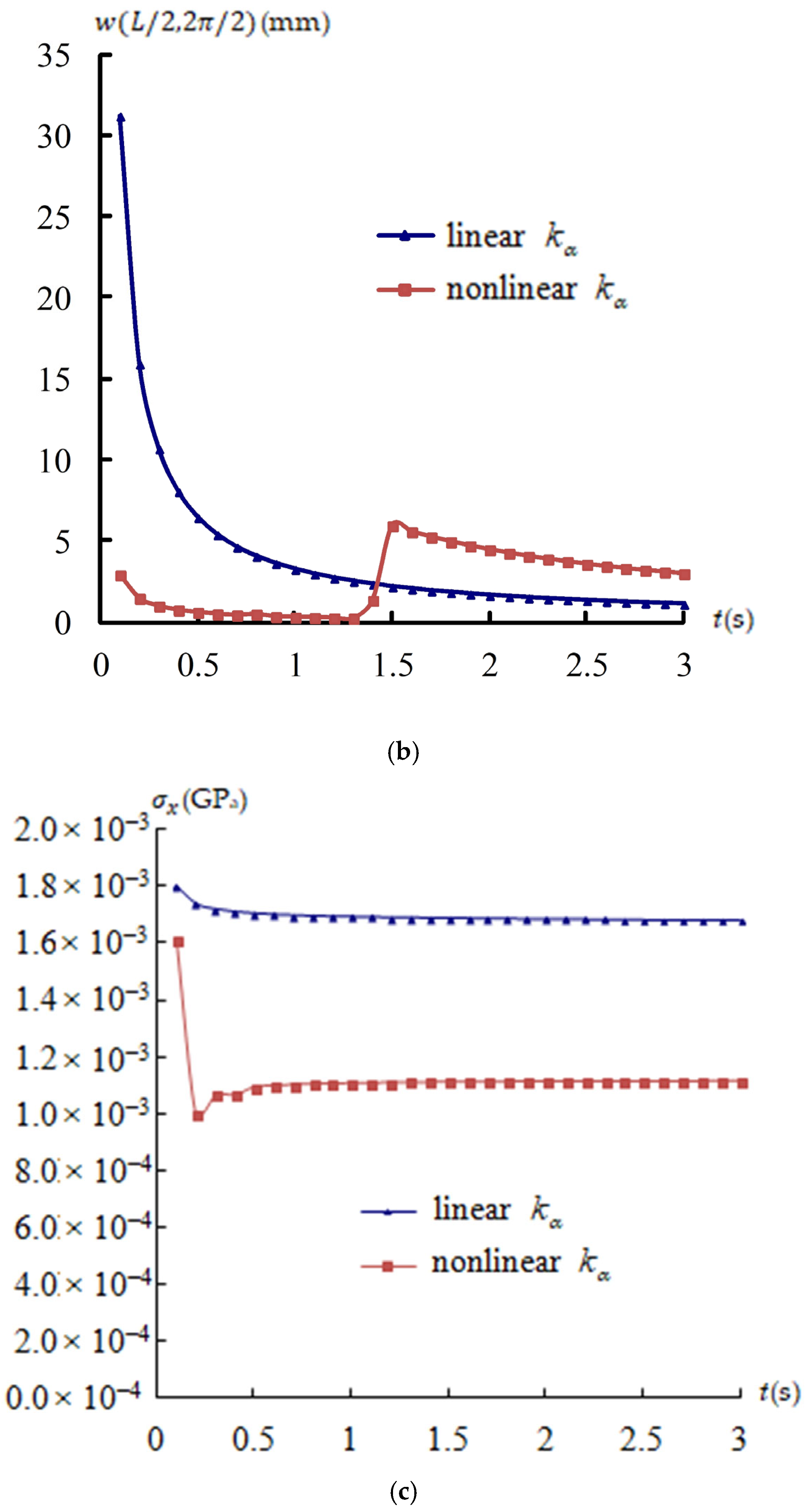
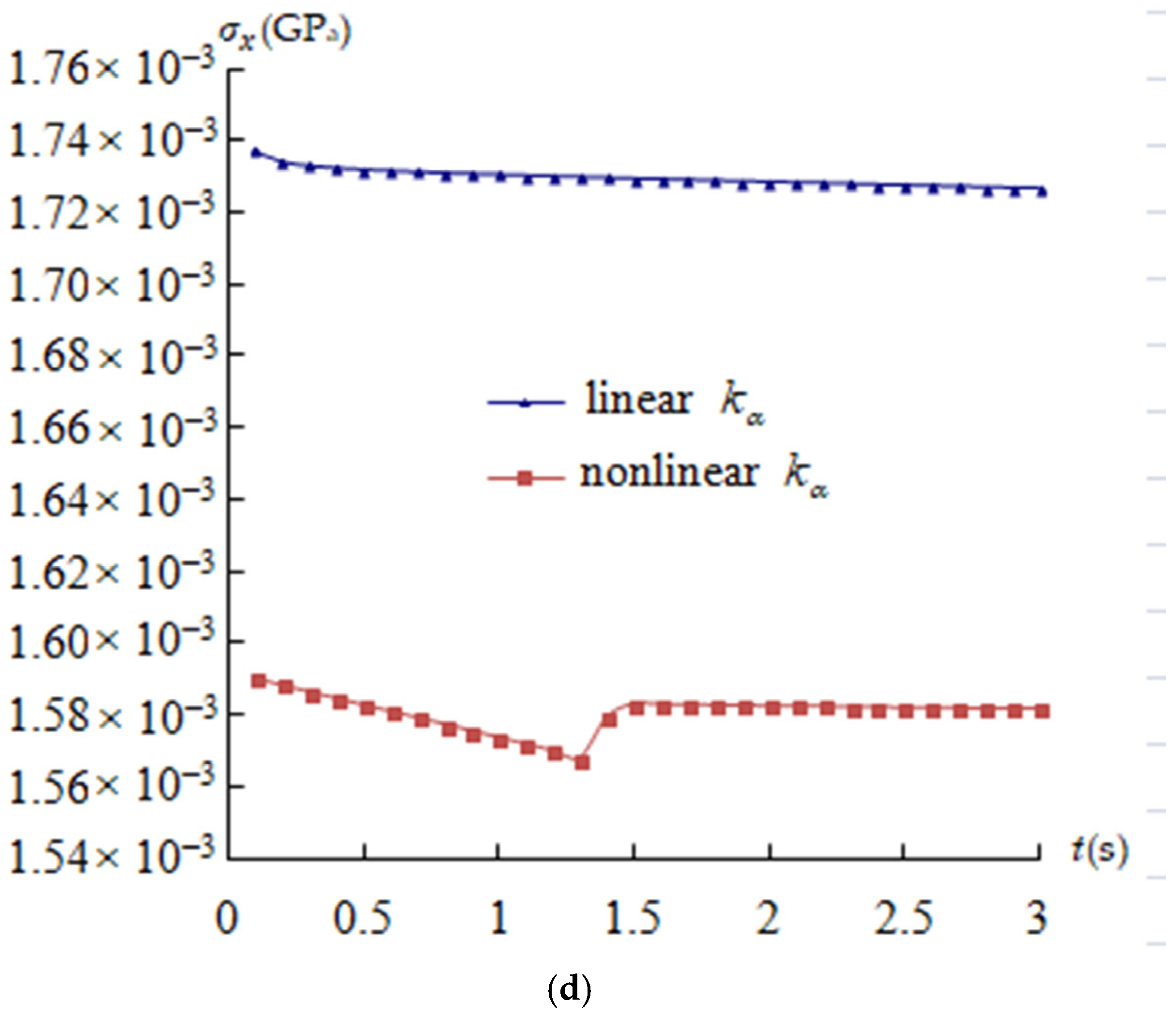
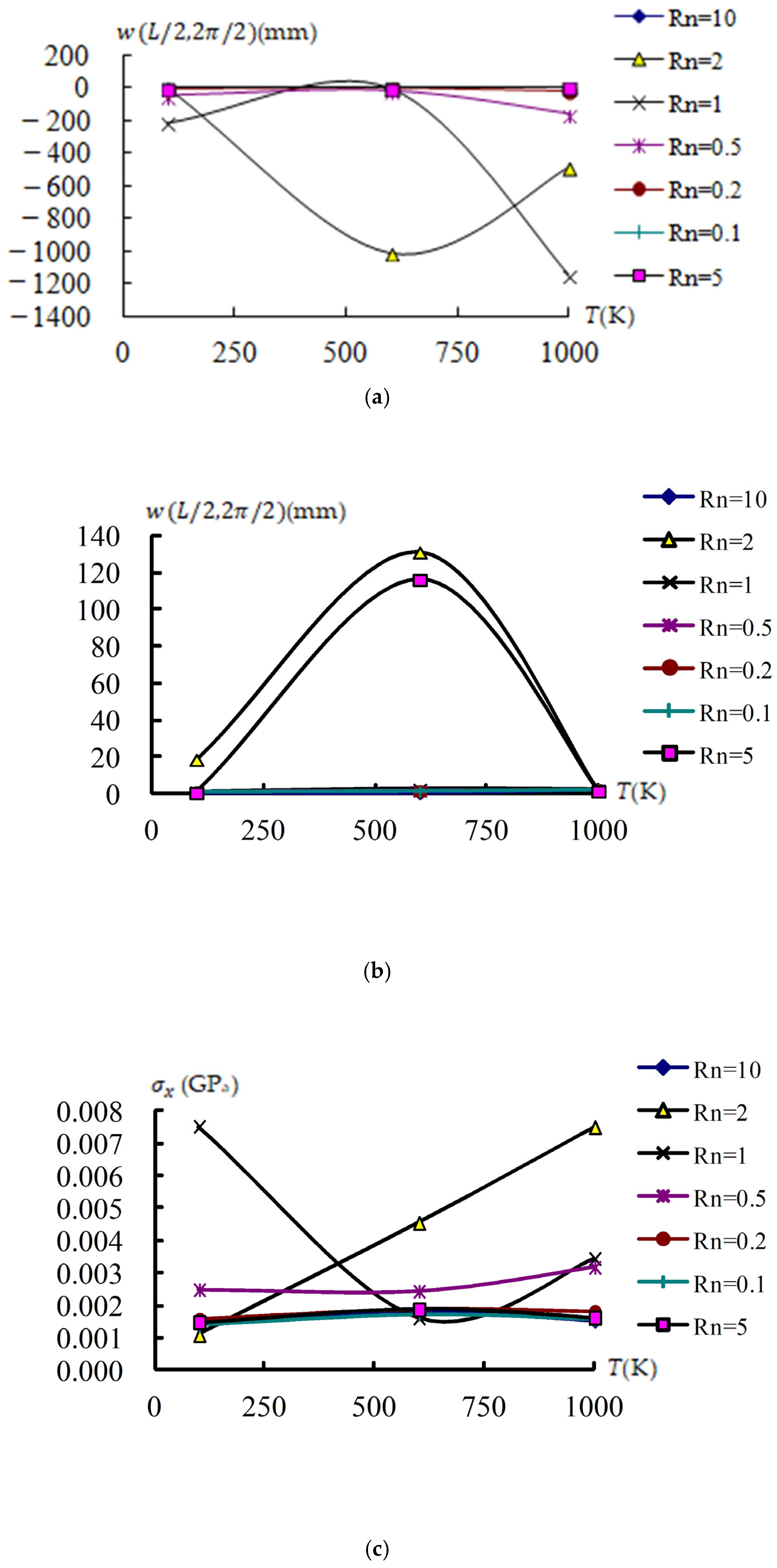
When a temperature gradient is involved in a material, then the transient thermal conduction is triggered. It is simply and ideally assumed that the temperature change follows the sinusoidal distribution for the TSDT displacements (5)–(7) and stresses (28). The response data of w ( L / 2 , 2 π / 2 ) (mm) and σ x (GPa) versus t (s) in the thermal sinusoidal vibration of TSDT for an FGM thick spherical shell on = 45 ° are calculated with advanced k α , γ and ω 11 . The γ values decrease from γ = 15.707960 rad/s at t = 0.1 s to γ = 0.523601 rad/s at t = 3.0 s for L / h = 5, and from γ = 15.707963 rad/s at t = 0.1 s to γ = 0.523599 rad/s at t = 3.0 s for L / h = 10. Figure 2 displays the data of w ( L / 2 , 2 π / 2 ) (mm) vs. t on nonlinear k α , linear k α for c 1 = 0.925925/mm2, L / h = 5, 10, R n = 1, T = 600 K, T ¯ 1 = 100 K and t = 0.1 s–3.0 s. Maximum w ( L / 2 , 2 π / 2 ) is 3.296229 mm provided on t = 0.2 s in nonlinear k α , L / h = 5, γ = 15.707964 rad/s. w ( L / 2 , 2 π / 2 ) data is in decreasing tendency vs. time for nonlinear k α , linear k α , L / h = 5. w ( L / 2 , 2 π / 2 ) data in linear k α is underestimated and smaller than that nonlinear k α on L / h = 5. Maximum w ( L / 2 , 2 π / 2 ) is 31.176647 mm provided on t = 0.1 s in linear k α , L / h = 10, γ = 15.707963 rad/s. w ( L / 2 , 2 π / 2 ) data is in decreasing tendency vs. time for linear k α , but have a jump into 5.920681 mm at t = 1.5 s in the nonlinear k α case for L / h = 10. w ( L / 2 , 2 π / 2 ) data in linear k α is overestimated and greater than that nonlinear k α during 0 s-1.5 s for L / h = 10. Also Figure 2 shows response data of dominated σ x (GPa) in center location on z = −0.5 h ,   =   45 ° , R n = 1, L / h = 5, 10, c 1 = 0.925925/mm2. The maximum σ x is 1.8011 × 10⁻³ GPa provided on t = 0.1 s in linear k α , L / h = 5. The σ x data shows a constant tendency vs. time in the nonlinear k α and linear k α cases at L / h = 5. The σ x data in the linear k α is overestimated and greater than that of the nonlinear k α for L / h = 5. The maximum σ x is 1.7368 × 10⁻³ GPa obtained at t = 0.1 s in the linear k α case at L / h = 10. The σ x data shows a constant tendency vs. time in the linear k α cases, but has a small jump into 1.5832 × 10⁻³ GPa at t = 1.5 s in the nonlinear k α case at L / h = 10. The σ x data in the linear k α case is overestimated and greater than that of the nonlinear k α case at L / h = 10. The discussion of practical insights for the nonlinear shear correction applied and considered in the computation of stress and displacement is very practical for thick-walled structures.
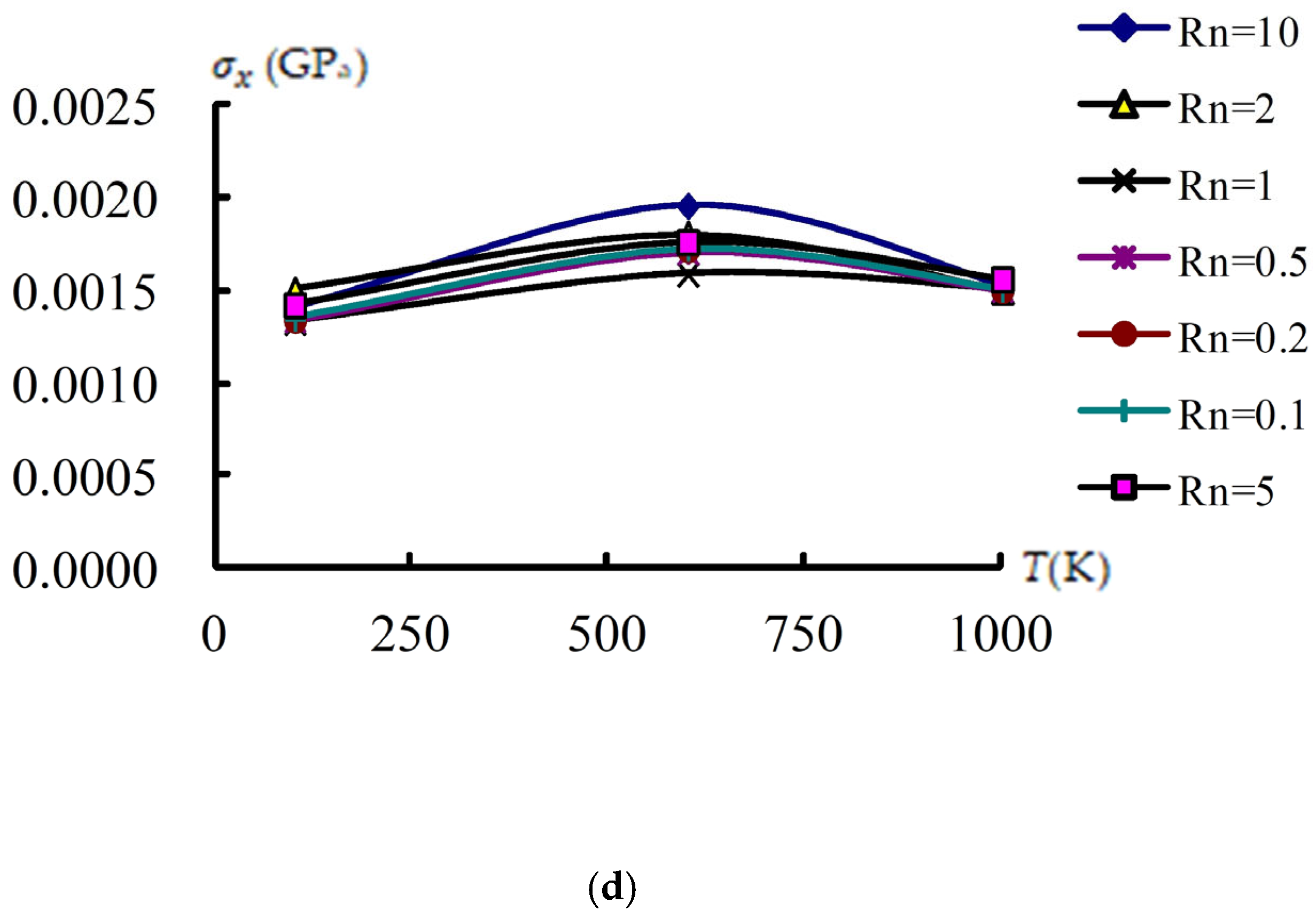
Figure 3 displays the data of w ( L / 2 , 2 π / 2 ) (mm) vs. T(K) and R n of the nonlinear TSDT under the values of c 1 = 0.925925/mm2,   =   45 ° , L / h = 5, 10 at T ¯ 1 = 100 K, ω 11 , γ and advanced k α at t = 0.1 s. The w ( L / 2 , 2 π / 2 ) data vs. T , R n , L / h = 5 case is shown; the maximum absolute w ( L / 2 , 2 π / 2 ) is −1144.055 mm, obtained at T = 1000 K, R n = 1. Large values of w ( L / 2 , 2 π / 2 ) data are provided from 600 K to 1000 K for R n = 1 and 2; w ( L / 2 , 2 π / 2 ) data at L / h = 5 can go on higher than 1000 K and R n = 2. The data of w ( L / 2 , 2 π / 2 ) vs. T , R n , L / h = 10, is in same lines except on R n = 2, 5, T = 600 K. The maximum w ( L / 2 , 2 π / 2 ) is 131.199188 mm obtained at T = 600 K, R n = 2. w ( L / 2 , 2 π / 2 ) data is in decreasing vs. T from 600 K to 1000 K on R n = 2, 5. w ( L / 2 , 2 π / 2 ) data on L / h = 10, R n = 2 and 5 can go on higher 1000 K, t = 0.1 s. Figure 3 also shows the normal stresses σ x (GPa) at the center location on z = −0.5 h vs. T , R n , = 45 ° , L / h = 5, 10. σ x data vs. T , R n , L / h = 5 is shown, σ x data vs. T is in increasing from 600 K to 1000 K on R n = 0.5, 1, 2. The maximum σ x is 7.5321 × 10⁻³ GPa obtained at T = 100 K, R n = 1. The σ x data at L / h = 5 can go on higher than 1000 K, except at R n = 0.5, 1, 2. The σ x data vs. T , R n , L / h = 10 is shown; the σ x data vs. T increases from 100 K to 600 K and decreases from 600 K to 1000 K on all R n . The maximum σ x is 1.96143 × 10⁻³ GPa obtained at T = 600 K, R n = 10. The σ x data at L / h = 10 can go on higher than 1000 K for all values of R n at t = 0.1 s. The discussion of practical insights for the temperature effect considered in the calculation of stress and displacement is very practical for FGM structures. Thus these material properties of FGMs can be used and are satisfied at higher temperatures.
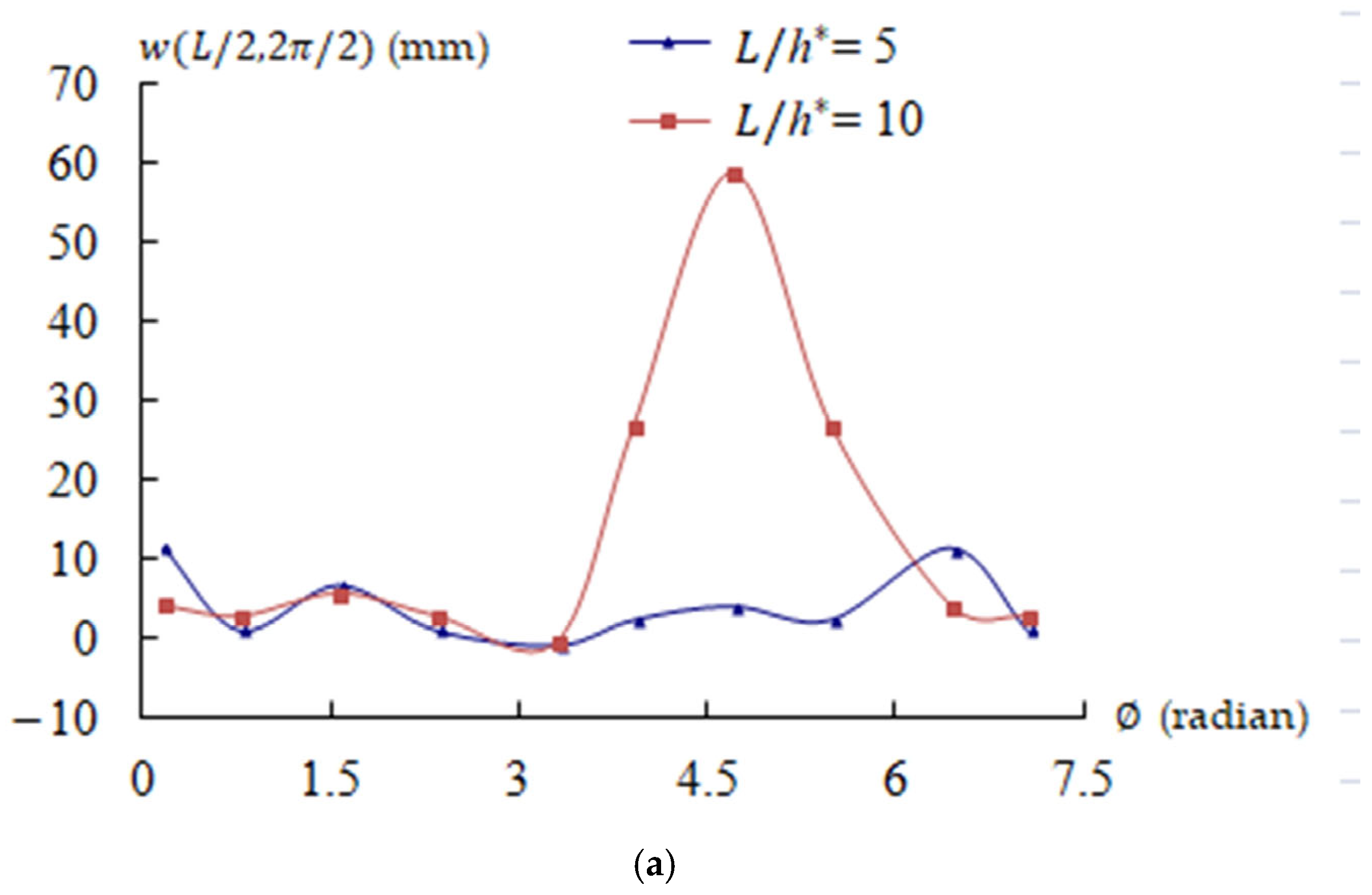
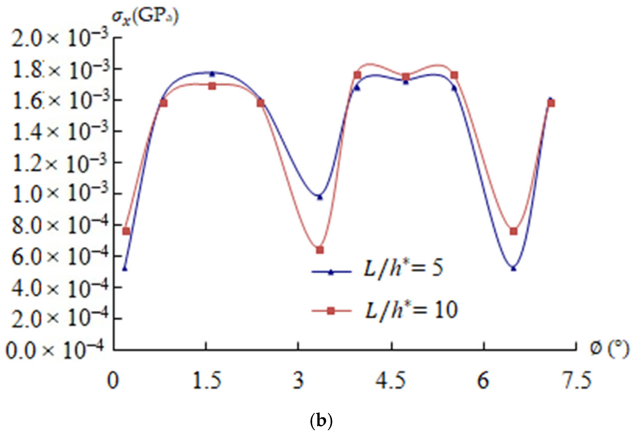
Figure 4 displays response data for w ( L / 2 , 2 π / 2 ) (mm) and σ x (GPa) vs. (radian) at L / h = 5, 10 for T = 600 K,   R n = 1, c 1 = 0.925925/mm2, T ¯ 1 = 100 K, γ values, advanced k α , and t = 0.1 s. The w ( L / 2 , 2 π / 2 ) data vs.   (radian) at L / h = 5, 10 are displayed; the w ( L / 2 , 2 π / 2 ) data at L / h = 10 oscillates sinusoidally similarly to the L / h = 5 case except for = 3.316125 radian-7.068583 radian. The response values of σ x at the center position of the inner surface vs. at L / h = 5, 10 are displayed; the σ x data at L / h = 5, 10 are sinusoidally oscillating similarly. The discussion of practical insights for the angle 0–90° between the z-axis and r considered in the calculation of stress and displacement is very practical for FGM structures.

3.3. Compared Results

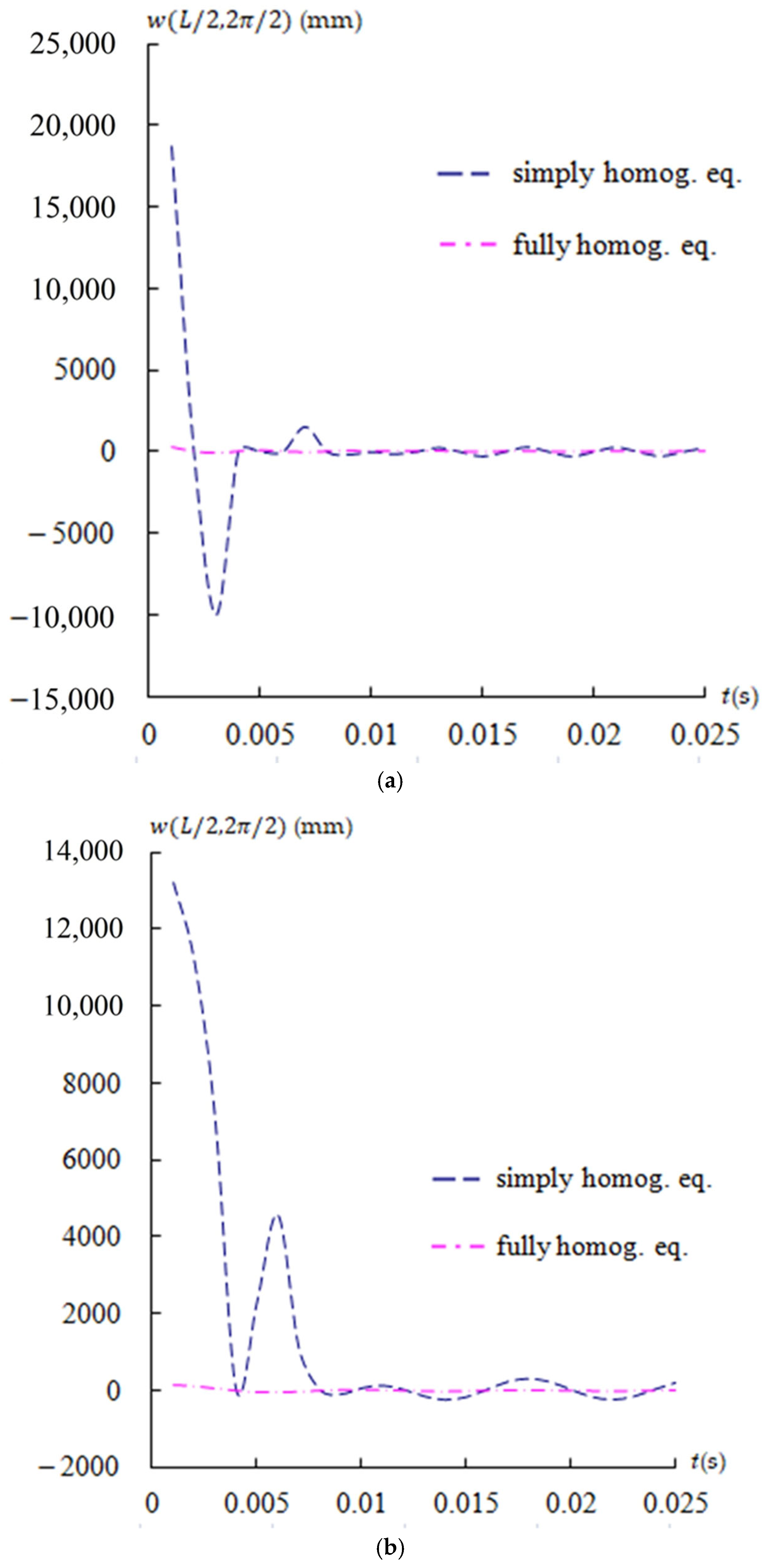
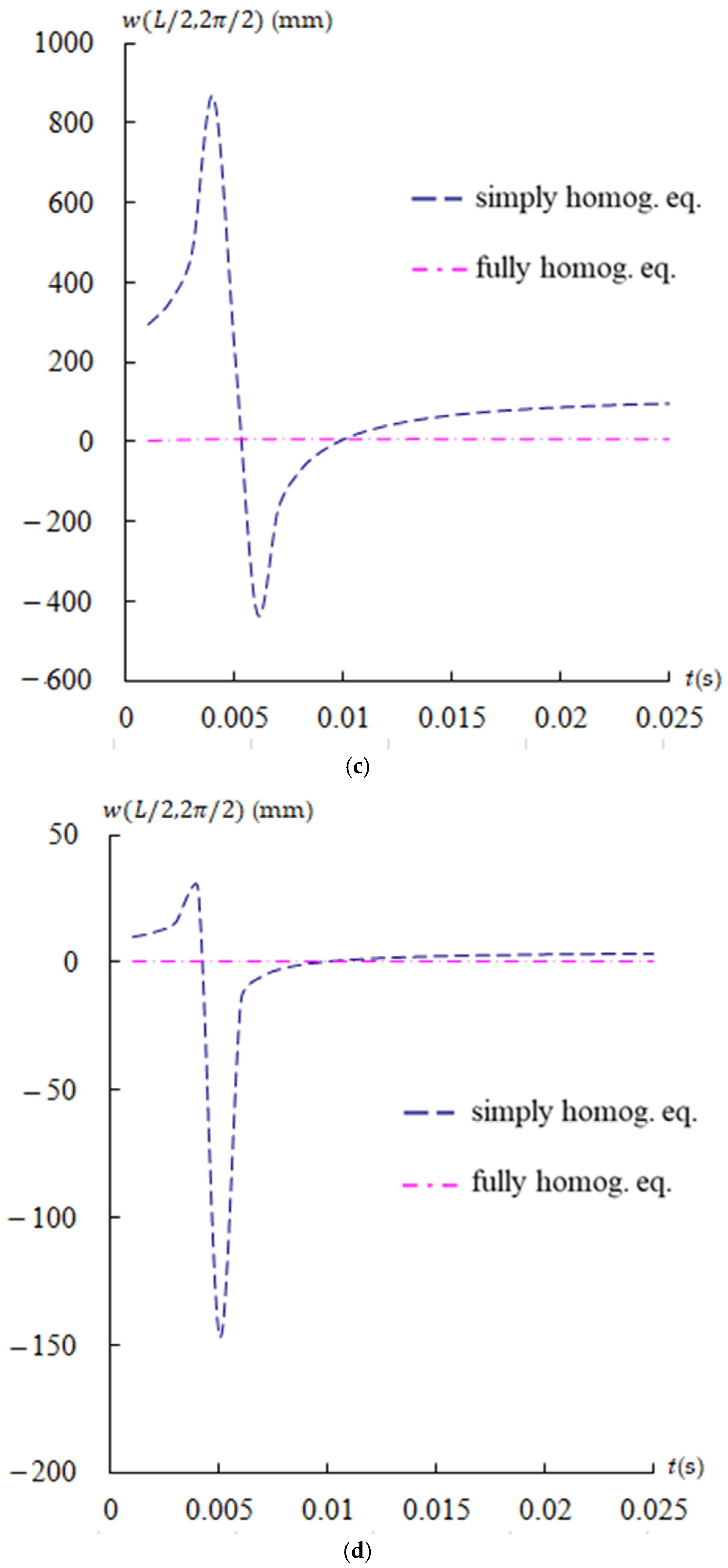
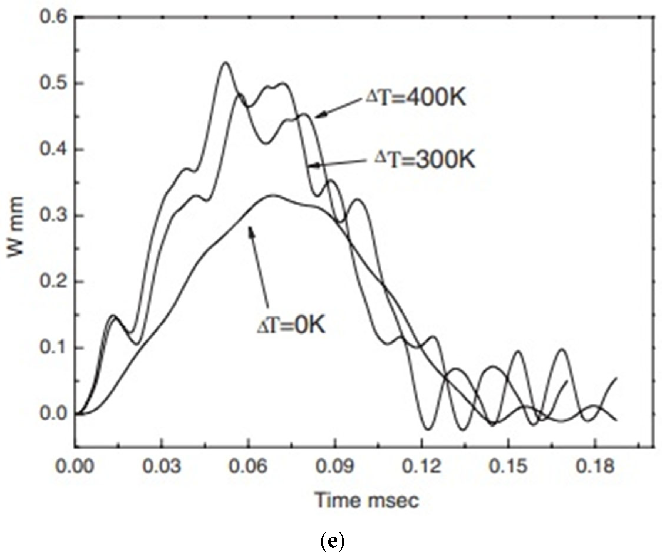
Figure 5 displays transient responses of compared w ( L / 2 , 2 π / 2 ) (mm) in FGM spherical shells for c 1 = 0.925925/mm2, L / h = 10,   =   45 ° , under the fixed ω 11 = 0.016792 rad/s approach of full algorithms and fixed ω 11 = 0.000592 rad/s approach of simple algorithms, respectively. We also used the fixed values of γ , R n = 1, advanced k α , T = 600 K and T ¯ 1 = 100 K for t = 0.001 s–0.025 s. Comparisons on w ( L / 2 , 2 π / 2 ) transient responses are shown in Figure 5a,b for full and simple algorithms with a super value of γ = 284,314.1 rad/s and with a high value of γ = 785.3982 rad/s. The transient values of center displacement amplitudes vs. higher γ are all oscillating and decreasing on L / h = 10. Comparisons on w ( L / 2 , 2 π / 2 ) transient responses are shown in Figure 5c,d for full and simple algorithms, respectively, with a lower value of γ = 15.707963 rad/s and with a less lower value of γ = 0.523599 rad/s. The transient values of center displacement amplitudes vs. γ are all greater in their values of rapidly oscillating and decreasing for the simple algorithm case than those for the full algorithm case. The numerical results are compared with similar published literature by Mao et al. (2011) [19] and displayed in Figure 5e on an FGM shallow spherical shell. The transient data of center displacement vs. t is oscillating and decreasing. The discussion of practical insights for full algorithms and simple algorithms considered in transient values of displacement is very practical for FGM structures under an applied heat flux frequency. Thus full algorithms can endure and be used for FGM structures under an applied heat flux frequency.
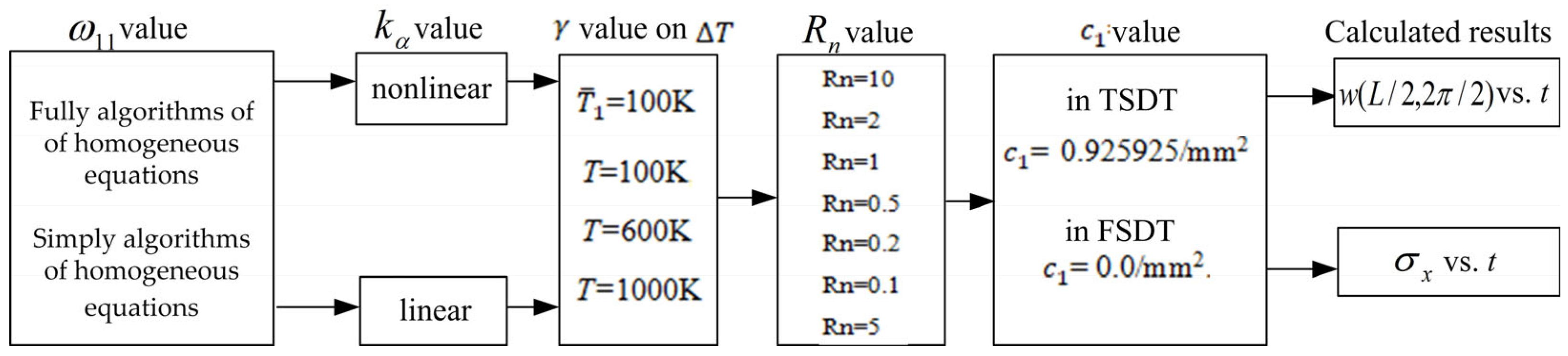
A brief graphical flow diagram is shown in Figure 6 for the computed results based on the ω 11 value in simple algorithms and full algorithms studies, and the γ value under T . The algorithms which are used for the following expressions
F H 13 = F H 14 = F H 15 = F H 23 = F H 24 = F H 25 = F H 31 = F H 32 = F H 41 = F H 42 = F H 51 = F H 52 = 0 ,
I 3 = J 1 = I 6 = J 4 = 0 ,
by substituting (36) and (37) into the elements of the fully homogeneous matrix [ F C m n ] of Equation (15) with subscripts m, n = 1,2,…,5, then the simply homogeneous matrix can be engaged. The ω 11 value is obtained from the simply and full algorithms to provide the initial vibration for FGMs. The FGMs are subjected to the thermal vibration load T with γ values. Thus the time response and transient response of w ( L / 2 , 2 π / 2 ) and σ x are computed and obtained.
Figure 6. Graphical flow diagram describing computed result based on simple and full algorithms and γ value under T .
Jcs 10 00360 g006

4. Discussions

To establish numerical validity with the data, future studies could process data from a simplified monolithic shell or an entire shell made of isotropic, linearly elastic materials. In future work, these practical applications could be applied to the fields of aircraft and missile for thick FGM spherical shells to obtain more detailed information. There is a limitation for thick FGM spherical shells under an applied thermal load T in linear vs. z on the (k)th layer in Equation (28); it would be welcomed and interesting to use an expression of nonlinear temperature rise vs. functions of z2 or z3 for the applied thermal load in next further studies to obtain more detailed information. It is reasonable to assume that expressions (36) and (37) are elements of the fully algorithmic matrix [ F C m n ] of Equation (15), thus a simplified algorithm can be obtained in Equation (38) in the following.
F H 11 λ m n F H 12 0       0 0 F H 12 F H 22 λ m n 0       0 0 0 0 F H 33 λ m n       F H 34 F H 35   0 0 F H 34       F H 44 K 2 λ m n I 0 F H 45   0 0 F H 35       F H 45 F H 55 K 2 λ m n I 0 a m n b m n c m n d m n e m n = 0 0 0 0 0 .

5. Conclusions

The computed results, which were prepared by GDQ approaches of thermal vibrations triggered by a sinusoidal temperature with frequency γ for obtaining data on the displacement and stress of a thick-walled FGM spherical shell, are presented by initially giving the natural frequency ω 11 with a fully algorithmic approach in Newton’s numerical method by using an advanced nonlinear shear correction k α and nonlinear TSDT term c 1 . Data of the center displacement and σ x in the linear k α are overestimated and greater than those in the nonlinear k α at L / h = 10. The center displacement amplitude at L / h = 5, 10 can go on higher than 1000 K of the environment at R n = 2. At t = 0.1 s, the stress σ x for the L / h = 5 case can reach temperatures higher than 1000 K of the environment, except for R n = 0.5, 1, 2; σ x for the L / h = 10 case can reach temperatures higher than 1000 K of the environment for all values of R n . The practical insights for the temperature effect considered in the calculation of stress and displacement is very clear and practical for the FGM spherical shell. The power law function property on the FGM spherical shell can be applied and is satisfied at higher temperature value environments.

Funding

This research received no external funding.

Data Availability Statement

Data are all available on request. The author declares that all the data are generated by the author, and also that data are openly available.

Acknowledgments

The author expresses his gratitude to the people helping with this work, and acknowledges the valuable suggestions from the peer reviewers.

Conflicts of Interest

The author declares no conflicts of interest.

Appendix A

The dynamic equilibrium differential equations in derivatives to u 0 , v 0 , w , ϕ x and ϕ θ of spherical shells are given as follows,
0 0 0 0 0 0 0 0 0 0 c 1 2 H 11 4 c 1 2 H 16 2 c 1 2 H 12 4 c 1 2 H 66 4 c 1 2 H 26 c 1 2 H 22 0 0 0 0 0 0 0 0 0 0 4 w x 4 1 R 4 w x 3 θ 1 R 2 4 w x 2 θ 2 1 R 3 4 w x θ 3 1 R 4 4 w θ 4 t + 0 0 0 0 0 0 0 0 c 1 E 11 3 c 1 E 16 c 1 E 12 2 c 1 E 66 c 1 E 26 0 0 0 0 0 0 0 0 c 1 E 16 c 1 E 12 2 c 1 E 66 3 c 1 E 26 c 1 E 22 c 1 E 11 3 c 1 E 16 c 1 E 12 + 2 c 1 E 66 c 1 E 26 c 1 E 16 c 1 E 12 + 2 c 1 E 66 3 c 1 E 26 c 1 E 22 0 0 0 0 0 0 0 0 0 0 0 0 c 1 F 11 + c 1 2 H 11 3 c 1 F 16 + 3 c 1 2 H 16 c 1 F 12 + c 1 2 H 12 2 c 1 F 66 + 2 c 1 2 H 66 c 1 F 26 + c 1 2 H 26 0 0 0 0 0 0 0 0 c 1 F 16 + c 1 2 H 16 2 c 1 F 66 + 2 c 1 2 H 66 c 1 F 12 + 2 c 1 2 H 12 3 c 1 F 26 + 3 c 1 2 H 26 c 1 F 22 + c 1 2 H 22 3 u 0 x 3 1 R 3 u 0 x 2 θ 1 R 2 3 u 0 x θ 2 1 R 3 3 u 0 θ 3 3 v 0 x 3 1 R 3 v 0 x 2 θ 1 R 2 3 v 0 x θ 2 1 R 3 3 v 0 θ 3 3 w x 3 1 R 3 w x 2 θ 1 R 2 3 w x θ 2 1 R 3 3 w θ 3 t + 0 0 0 0 0 0 0 0 0 0 0 0 0 0 0 0 c 1 F 11 c 1 2 H 11 3 c 1 F 16 3 c 1 2 H 16 2 c 1 F 66 2 c 1 2 H 66 + c 1 F 12 c 1 2 H 12 c 1 F 26 c 1 2 H 26 c 1 F 16 c 1 2 H 16 c 1 F 12 c 1 2 H 12 + 2 c 1 F 66 2 c 1 2 H 66 3 c 1 F 26 3 c 1 2 H 26 c 1 F 22 c 1 2 H 22 0 0 0 0 0 0 0 0 0 0 0 0 0 0 0 0 3 ϕ x x 3 1 R 3 ϕ x x 2 θ 1 R 2 3 ϕ x x θ 2 1 R 3 3 ϕ x θ 3 3 ϕ θ x 3 1 R 3 ϕ θ x 2 θ 1 R 2 3 ϕ θ x θ 2 1 R 3 3 ϕ θ θ 3 t + A 11 2 A 16 A 66 A 16 A 12 + A 66 A 26 0 0 0 A 16 A 12 + A 66 A 26 A 66 2 A 26 A 22 0 0 0 0 0 0 0 0 0 3 c 1 ( 2 D 55 3 c 1 F 55 ) + A 55 + c 1 2 I 6 2 t 2 6 c 1 ( 2 D 45 3 c 1 F 45 ) + 2 A 45 3 c 1 ( 2 D 44 3 c 1 F 44 ) + A 44 + c 1 2 I 6 2 t 2 B 11 c 1 E 11 2 B 16 2 c 1 E 16 B 66 c 1 E 66 B 16 c 1 E 16 B 12 + B 66 c 1 E 12 c 1 E 66 B 26 c 1 E 26 0 0 0 B 16 c 1 E 16 B 12 + B 66 c 1 E 12 c 1 E 66 B 26 c 1 E 26 B 66 c 1 E 66 2 B 26 2 c 1 E 26 B 22 c 1 E 22 0 0 0 2 u 0 x 2 1 R 2 u 0 x θ 1 R 2 2 u 0 θ 2 2 v 0 x 2 1 R 2 v 0 x θ 1 R 2 2 v 0 θ 2 2 w x 2 1 R 2 w x θ 1 R 2 2 w θ 2 t + B 11 c 1 E 11 2 B 16 2 c 1 E 16 B 66 c 1 E 66 B 16 c 1 E 16 B 12 + B 66 c 1 E 12 c 1 E 66 B 26 c 1 E 26 B 16 c 1 E 16 B 12 + B 66 c 1 E 12 c 1 E 66 B 26 c 1 E 26 B 66 c 1 E 66 2 B 26 2 c 1 E 26 B 22 c 1 E 22 0 0 0 0 0 0 D 11 2 c 1 F 11 + c 1 2 H 11 2 D 16 4 c 1 F 16 + 2 c 1 2 H 16 D 66 2 c 1 F 66 + c 1 2 H 66 D 16 2 c 1 F 16 + c 1 2 H 16 D 12 + D 66 2 c 1 F 12 + c 1 2 H 12 2 c 1 F 66 + c 1 2 H 66 D 26 2 c 1 F 26 + c 1 2 H 26 D 16 2 c 1 F 16 + c 1 2 H 16 D 12 + D 66 2 c 1 F 12 + c 1 2 H 12 2 c 1 F 66 + c 1 2 H 66 D 26 2 c 1 F 26 + c 1 2 H 26 D 66 2 c 1 F 66 + c 1 2 H 66 2 D 26 4 c 1 F 26 + 2 c 1 2 H 26 D 22 2 c 1 F 22 + c 1 2 H 22 2 ϕ x x 2 1 R 2 ϕ x x θ 1 R 2 2 ϕ x θ 2 2 ϕ θ x 2 1 R 2 ϕ θ x θ 1 R 2 2 ϕ θ θ 2 t 0 0 0 0 c 1 I 3 2 t 2 0 0 0 0 0 0 0 0 0 0 c 1 I 3 2 t 2 0 0 0 0 c 1 I 3 2 t 2 u 0 R ( A 55 3 c 1 D 55 ) u 0 R ( A 45 3 c 1 D 45 ) v 0 R ( A 45 3 c 1 D 45 ) c 1 I 3 2 t 2 v 0 R ( A 44 3 c 1 D 44 ) 0 0 A 55 6 c 1 D 55 + 9 c 1 2 F 55 c 1 J 4 2 t 2 A 45 6 c 1 D 45 + 9 c 1 2 F 45 A 45 6 c 1 D 45 + 9 c 1 2 F 45 A 44 6 c 1 D 44 + 9 c 1 2 F 44 c 1 J 4 2 t 2 0 0 0 0 6 c 1 D 55 9 c 1 2 F 55 A 55 + c 1 J 4 2 t 2 6 c 1 D 45 9 c 1 2 F 45 A 45 0 0 0 0 0 0 0 0 6 c 1 D 45 9 c 1 2 F 45 A 45 6 c 1 D 44 9 c 1 2 F 44 A 44 + c 1 J 4 2 t 2 0 0 0 0 u 0 x 1 R u 0 θ v 0 x 1 R v 0 θ w x 1 R w θ ϕ x x 1 R ϕ x θ ϕ θ x 1 R ϕ θ θ t + I 0 2 t 2                       0                       0                         J 1 2 t 2                           0     0                         I 0 2 t 2                   0                               0                   J 1 2 t 2   0                                 0                   I 0 2 t 2                       0                             0 J 1 2 t 2 1 R s i n       1 R s i n ( A 45     0               A 55 + 6 c 1 D 55       A 45 + 6 c 1 D 45 A 55 + 3 c 1 D 55           + 3 c 1 D 45 )                 9 c 1 2 F 55 K 2 2 t 2     9 c 1 2 F 45     1 R s i n           J 1 2 t 2 1 R s i n           0           A 45 + 6 c 1 D 45     A 44 + 6 c 1 D 44     A 45 + 3 c 1 D 45       A 44 + 3 c 1 D 44           9 c 1 2 F 45             9 c 1 2 F 44 K 2 2 t 2 u 0 v 0 w ϕ x ϕ θ = f 1 f 2 f 3 f 4 f 5 ,
in which   f 1 = N ¯ x x x + 1 R N ¯ x θ θ + p 1 ,
f 2 = N ¯ x θ x + 1 R N ¯ θ θ θ + p 2 ,
f 3 = q + c 1 ( 2 P ¯ x x x 2 + 2 R 2 P ¯ x θ x θ + 1 R 2 2 P ¯ θ θ θ 2 ) ,
f 4 = M ¯ ˜ x x x + 1 R M ¯ ˜ x θ θ c 1 ( P ¯ x x x + 1 R P ¯ x θ θ ) ,
f 5 = M ¯ ˜ x θ x + 1 R M ¯ ˜ θ θ θ c 1 ( P ¯ x θ x + 1 R P ¯ θ θ θ ) ,
N ¯ x x , M ¯ ~ x x , P ¯ x x = h 2 h 2 Q ¯ 11 α x + Q ¯ 12 α θ + Q ¯ 16 α x θ Δ T ( 1 , z , z 3 ) d z ,
N ¯ θ θ , M ¯ ~ θ θ , P ¯ θ θ = h 2 h 2 Q ¯ 12 α x + Q ¯ 22 α θ + Q ¯ 26 α x θ Δ T ( 1 , z , z 3 ) d z , N ¯ x θ , M ¯ ~ x θ , P ¯ x θ = h 2 h 2 Q ¯ 16 α x + Q ¯ 26 α θ + Q ¯ 66 α x θ Δ T ( 1 , z , z 3 ) d z ,
T = z h T ¯ 1 s i n ( π x / L ) s i n ( π θ ) s i n ( γ t ) ,
where γ is the applied heat flux frequency, T ¯ 1 is the temperature amplitude ,   p 1 and p 2 are the external in-plane distributed forces in the x and θ direction, respectively, and q is the external pressure load.
The detailed F C m n are listed as follows,
F C 14 = F H 14 J 1 λ m n I 0 ,
F C 15 = F H 15 ,
F C 21 = F H 12 ,
F C 22 = F H 22 I 0 λ m n I 0 ,
F C 23 = F H 23 + c 1 I 3 n π R λ m n I 0 ,
F C 24 = F H 24 ,
F C 25 = F H 25 J 1 λ m n I 0 ,
F C 31 = F H 13 + c 1 I 3 m π L λ m n I 0 ,
F C 32 = F H 23 + c 1 I 3 n π R λ m n I 0 ,
F C 33 = F H 33 [ I 0 + c 1 2 I 6 m π L 2 + c 1 2 I 6 n π R 2 ] λ m n / I 0 ,
F C 34 = F H 34 + c 1 J 4 m π L λ m n I 0 ,
F C 35 = F H 35 + c 1 J 4 n π R λ m n I 0 ,
F C 41 = F H 14 J 1 λ m n I 0 ,
F C 42 = F H 24 ,
F C 43 = F H 34 + c 1 J 4 m π L λ m n I 0 ,
F C 44 = F H 44 K 2 λ m n I 0 ,
F C 45 = F H 45 ,
F C 51 = F H 15 ,
F C 52 = F H 25 J 1 λ m n I 0 ,
F C 53 = F H 35 + c 1 J 4 n π R λ m n I 0 ,
F C 54 = F H 45 ,
F C 55 = F H 55 K 2 λ m n I 0 ,
The detailed F H m n are listed as follows,
F H 13 = c 1 E 11 ( m π / L ) 3 ( c 1 E 12 + 2 c 1 E 66 ) ( m π / L ) ( n π / R ) 2 ,
F H 14 = ( B 11 c 1 E 11 ) ( m π / L ) 2 + ( B 66 c 1 E 66 ) ( n π / R ) 2 ,
F H 15 = ( B 12 + B 66 c 1 E 12 c 1 E 66 ) ( m π / L ) ( n π / R ) ,
F H 22 = A 66 ( m π / L ) 2 + A 22 ( n π / R ) 2 ,
F H 23 = ( c 1 E 12 + 2 c 1 E 66 ) ( m π / L ) 2 ( n π / R ) c 1 E 22 ( n π / R ) 3 ,
F H 24 = ( B 12 + B 66 c 1 E 12 c 1 E 66 ) ( m π / L ) ( n π / R ) ,
F H 25 = ( B 66 c 1 E 66 ) ( m π / L ) 2 + ( B 22 c 1 E 22 ) ( n π / R ) 2 ,
F H 33 = A 55 ( m π / L ) 2 + A 44 ( n π / R ) 2 +   c 1 2 H 11 ( m π / L ) 4 + ( 2 c 1 2 H 12 + 4 c 1 2 H 66 ) ( m π / L ) 2 ( n π / R ) 2 +   c 1 2 H 22 ( n π / R ) 4 3 c 1 ( 2 D 55 3 c 1 F 55 ) ( m π / L ) 2   3 c 1 ( 2 D 44 3 c 1 F 44 ) ( n π / R ) 2 ,
F H 34 = A 55 m π / L ( c 1 F 11 c 1 2 H 11 ) ( m π / L ) 3   ( 2 c 1 F 66 2 c 1 2 H 66 + c 1 F 12 c 1 2 H 12 ) ( m π / L ) ( n π / R ) 2 ( 6 c 1 D 55 9 c 1 2 F 55 ) ( m π / L ) ,
F H 35 = A 44 n π / R ( c 1 F 22 c 1 2 H 22 ) ( n π / R ) 3   ( 2 c 1 F 66 2 c 1 2 H 66 + c 1 F 12 c 1 2 H 12 ) ( m π / L ) 2 ( n π / R ) ( 6 c 1 D 44 9 c 1 2 F 44 ) ( n π / R ) ,
F H 44 = ( D 11 2 c 1 F 11 + c 1 2 H 11 ) ( m π / L ) 2 + ( D 66 2 c 1 F 66 + c 1 2 H 66 ) ( n π / R ) 2 + A 55 6 c 1 D 55 + 9 c 1 2 F 55 ,
F H 45 = ( D 12 + D 66 2 c 1 F 12 + c 1 2 H 12 2 c 1 F 66 + c 1 2 H 66 ) ( m π / L ) ( n π / R ) ,
F H 55 = ( D 66 2 c 1 F 66 + c 1 2 H 66 ) ( m π / L ) 2 + ( D 22 2 c 1 F 22 + c 1 2 H 22 ) ( n π / R ) 2 + A 44 6 c 1 D 44 + 9 c 1 2 F 44

References

  1. Li, Y. Study of impact dynamics of porous brittle materials based on a three-dimensional lattice point-spring model. Appl. Math. Model. 2023, 124, 678–693. [Google Scholar]
  2. Keibolahi, A.; Kiani, Y.; Eslami, M.R. Nonlinear dynamic snap-through and vibrations of temperature-dependent FGM deep spherical shells under sudden thermal shock. Thin-Walled Struct. 2023, 185, 110561. [Google Scholar] [CrossRef]
  3. Sorohan, S.; Constantinescu, D.M. Tailoring of functionally graded spheres using a uniform stress condition. Rom. J. Tech. Sci. Appl. Mech. 2023, 68, 1. [Google Scholar] [CrossRef]
  4. Tamnar, R.B.; Sayyad, A.S. Static response of functionally graded porous spherical shells using trigonometric shear deformation theory. Mater. Res. Proc. 2023, 31, 76–85. [Google Scholar] [CrossRef]
  5. De Pascalis, R. Diffusion-induced stress in a functionally graded incompressible elastic sphere. Int. J. Non-Linear Mech. 2022, 138, 103850. [Google Scholar] [CrossRef]
  6. Flis, J.; Muc, A. Influence of coupling effects on analytical solutions of functionally graded (FG) spherical shells of revolution. Rev. Adv. Mate. Sci. 2021, 60, 761–770. [Google Scholar] [CrossRef]
  7. Zannon, M.; Abu-Rqayiq, A.; Al-bdour, A. Free vibration analysis of thick FGM spherical shells based on a third-order shear deformation theory. Eur. J. Pure Appl. Math. 2020, 13, 766–778. [Google Scholar] [CrossRef]
  8. Khinchi, A.; Sharma, P. Review on vibration analysis of functionally graded material (FGM) spherical shell. In Proceedings of the 14th International Conference on Recent trends in Engineering, Appl. Sci. and Manage (ICRTESM-19), Bundi, India, 16–17 February 2019; pp. 95–101. [Google Scholar]
  9. Shahmohamadi, M.A.; Kabir, M.Z. Effects of shear deformation on mechanical and thermo-mechanical nonlinear stability of FGM shallow spherical shells subjected to uniform external pressure. Sci. Iran. A 2017, 24, 584–596. [Google Scholar] [CrossRef][Green Version]
  10. Duc, N.D.; Quang, V.D.; Anh, V.T.T. The nonlinear dynamic and vibration of the S-FGM shallow spherical shells resting on an elastic foundations including temperature effects. Int. J. Mech. Sci. 2017, 123, 54–63. [Google Scholar] [CrossRef]
  11. Hong, C.C. GDQ computation for thermal vibration of thick FGM plates by using third-order shear deformation theory. Mater. Sci. Eng. B 2023, 294, 116208. [Google Scholar] [CrossRef]
  12. Hong, C.C. Advanced dynamic thermal vibration of thick composited FGM cylindrical shells with fully homogeneous equation by using TSDT and nonlinear varied shear coefficient. J. Compos. Sci. 2025, 9, 4. [Google Scholar]
  13. Hong, C.C. Thermal vibration of thick FGM spherical shells by using TSDT. Int. J. Mech. Mater. Des. 2021, 17, 367–380. [Google Scholar] [CrossRef]
  14. Bagheri, H.; Kiani, Y.; Eslami, M.R. Application of GDQ method to large amplitude response of FGM joined spherical-conical shells under rapid surface heating. Mech. Based Des. Struct. Mach. 2024, 52, 5. [Google Scholar]
  15. Kareem, M.G.; Al-Raheem, S.K.; Sadiq, S.E.; Alansari, L.S. Review of research on the vibration and buckling of functionally graded spherical shells. Int. J. Sci. Res. Arch. 2024, 13, 2170–2186. [Google Scholar] [CrossRef]
  16. Javani, M.; Kiani, Y.; Sadighi, M.; Eslami, M.R. Nonlinear vibration behavior of rapidly heated temperature-dependent FGM shallow spherical shells. AIAA J. 2019, 57, 9. [Google Scholar] [CrossRef]
  17. Pang, F.; Gao, C.; Cui, J.; Ren, Y.; Li, H.; Wang, H. A semianalytical approach for free vibration characteristics of functionally graded spherical shell based on first-order shear deformation theory. Shock Vib. 2019, 2019, 7352901. [Google Scholar]
  18. Sondhi, L.; Sahu, R.K.; Bhowmick, S.; Thawait, A.K. Thermo–elastic stresses and deformation analysis of FG rotating hollow spherical body. Mech. Adv. Compos. Struct. 2022, 9, 125–136. [Google Scholar]
  19. Mao, Y.Q.; Fu, Y.M.; Chen, C.P.; Li, Y.L. Nonlinear dynamic response for functionally graded shallow spherical shell under low velocity impact in thermal environment. Appl. Math. Model. 2011, 35, 2887–2900. [Google Scholar] [CrossRef]
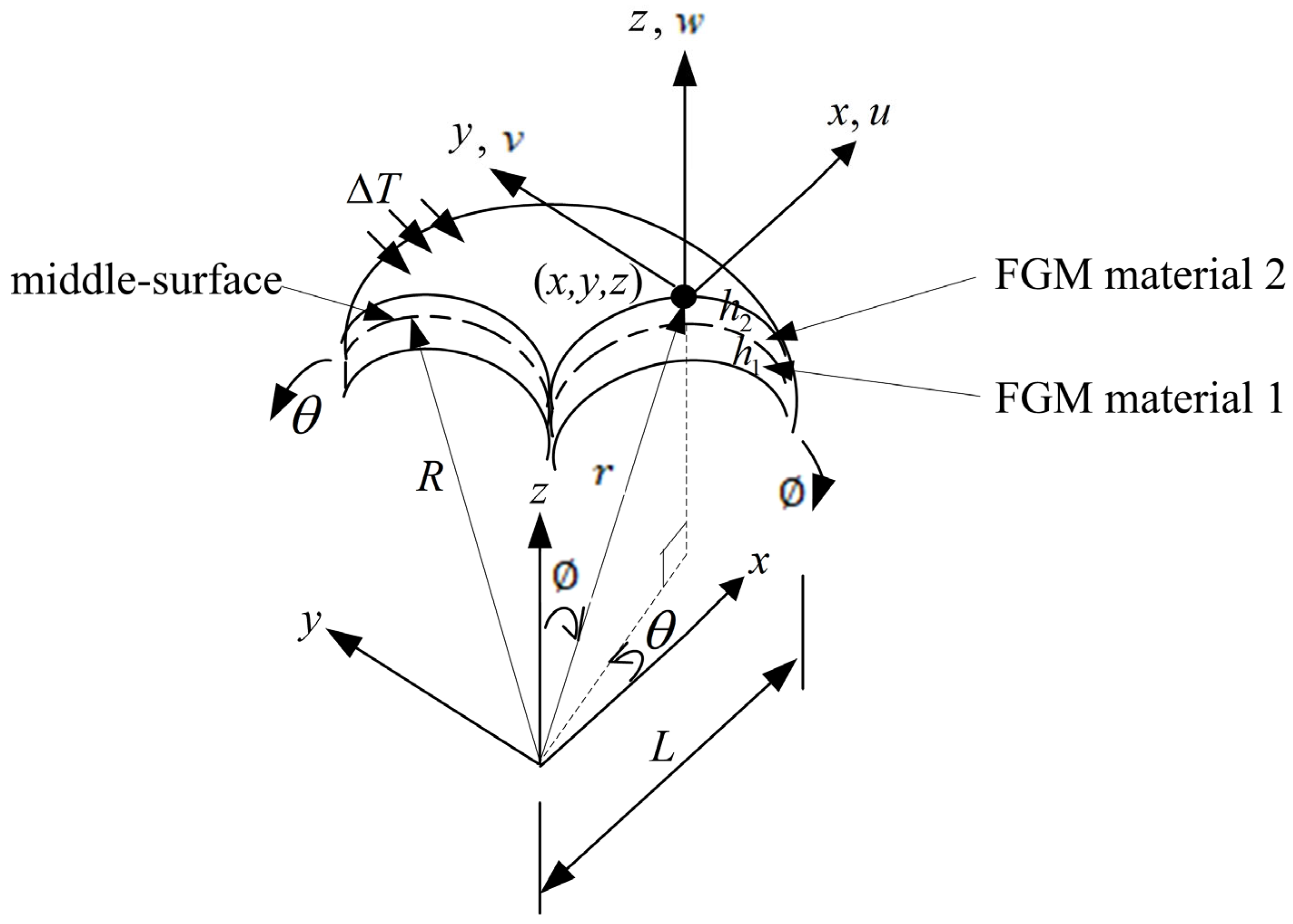
Figure 1. Constituent materials of thick-walled FGMs in L = R , θ = 0 ~ 2 π geometries of spherical shells subjected to thermal-load T .
Jcs 10 00360 g001
Figure 2. Advanced w ( L / 2 , 2 π / 2 ) (mm) and σ x (GPa) vs. t(s) on = 45 ° for: (a) w ( L / 2 , 2 π / 2 ) (mm) vs. t(s) for L / h = 5; (b) w ( L / 2 , 2 π / 2 ) (mm) vs. t(s) for L / h = 10; (c) σ x (GPa) vs. t(s) for L / h = 5; (d) σ x (GPa) vs. t(s) for L / h = 10 .
Jcs 10 00360 g002aJcs 10 00360 g002bJcs 10 00360 g002c
Figure 3. Advanced w ( L / 2 , 2 π / 2 ) (mm) versus T(K) and σ x (GPa) versus T(K) on = 45 ° for: (a) w ( L / 2 , 2 π / 2 ) (mm) versus T(K), L / h = 5; (b) w ( L / 2 , 2 π / 2 ) (mm) versus T(K), L / h = 10; (c) σ x (GPa) versus T(K), L / h = 5; (d) σ x (GPa) versus T(K), L / h = 10.
Jcs 10 00360 g003aJcs 10 00360 g003b
Figure 4. Advanced w ( L / 2 , 2 π / 2 ) (mm) and σ x (GPa) versus (radian) for: (a) w ( L / 2 , 2 π / 2 ) (mm) vs. (radian) on L / h = 5, 10; (b) σ x (GPa) versus (radian) on L / h = 5, 10.
Jcs 10 00360 g004aJcs 10 00360 g004b
Figure 5. Transient w ( L / 2 , 2 π / 2 ) (mm) versus t(s) compared under fully and simply equations of algorithms for: (a) γ = 284314.1 rad/s; (b) γ = 785.3982 rad/s; (c) γ = 15.707963 rad/s; (d) γ = 0.523599 rad/s; (e) compared numerical results by Mao et al. (2011) [19].
Jcs 10 00360 g005aJcs 10 00360 g005bJcs 10 00360 g005c
Table 1. Values of temperature coefficients P 0 , P 1 , P 1 , P 2 , P 3 for mechanical properties.
Material P i P 0 P 1 P 1 P 2 P 3
SUS304 E 1 (Pa)201.04 × 10903.079 × 10−4−6.534 × 10−70
ν 1 0.32620−2.002 × 10−43.797 × 10−70
ρ 1 (kg/m3)81660000
α 1 (K−1)12.33 × 10−608.086 × 10−400
κ 1 (W/(mK))15.3790000
C v 1 (J/(kgK))496.560−1.151 × 10−31.636 × 10−6−5.863 × 10⁻¹⁰
Si3N4 E 2 (Pa)348.43 × 1090−3.70 × 10−42.16 × 10−7−8.946 × 10⁻¹¹
ν 2 0.240000
ρ 2 (kg/m3)23700000
α 2 (K−1)5.8723 × 10−609.095 × 10−400
κ 2 (W/(mK))13.7230000
C v 2 (J/(kgK))555.1101.016 × 10−32.92 × 10⁻⁷−1.67 × 10⁻¹⁰
Table 2. Typical values of ω 11 vs. c 1 , T , R n provided on L / h = 5, = 10 ° .
c 1
(1/mm2)
T
(K)
ω 11 (rad/s)
on R n = 0.5
ω 11 (rad/s)
on R n = 2
0.9259251000.0011770.002203
6000.0008650.007157
10000.0023890.001480
01000.0163280.017524
6000.0173950.018486
10000.0187700.020655
Table 3. FGM spherical shells convergence in TSDT, advanced k α on   =   10 ° .
c 1
(1/mm2)
GDQ Grids
N × M
w ( L / 2 , 2 π / 2 )
on R n = 0.5
w ( L / 2 , 2 π / 2 )
on R n = 2
0.9259257 × 70.1769750.022818
9 × 90.1803530.022844
11 × 110.1803250.022844
13 × 130.1804050.022842
0.7 × 70.0116080.009611
9 × 90.0116110.009614
11 × 110.0116110.009614
13 × 130.0116110.009613
Disclaimer/Publisher’s Note: The statements, opinions and data contained in all publications are solely those of the individual author(s) and contributor(s) and not of MDPI and/or the editor(s). MDPI and/or the editor(s) disclaim responsibility for any injury to people or property resulting from any ideas, methods, instructions or products referred to in the content.