Machine Learning-Based Prediction of EDM Material Removal Rate and Surface Roughness

Abstract

Examining the electrical discharge machining (EDM) process is challenging in manufacturing technology due to the complexity of the physical events that take place in the gaps between electrodes. In this study, we examined the EDM process in detail and developed multiple machine learning (ML) models to describe the relationship between the EDM independent (process parameters) and dependent (responses) variables. The collected experimental data was used to train the machine learning models. According to the results, the GPR model outperformed other ML models across different materials, with average RMSE values of 0.9234 and 3.0216 for the material removal rate (MRR) and surface roughness (Sa), respectively, highlighting the effectiveness of ML tools at modeling complex machining processes, such as EDM. In addition, as a practical implication, this study opens the door to employing the developed ML models to predict the EDM process performance.

1. Introduction

The integration of machine learning algorithms can improve machine productivity and efficiency. Machine learning algorithms can be applied to both conventional and non-conventional processes to predict and improve the process parameters, tool condition monitoring, error detection, and product quality, thereby enhancing the efficiency of manufacturing processes in the industry. Machine learning applications in manufacturing have benefits when it comes to dealing with complex, massive dimensionality and identifying hidden relationships in both small and large datasets, which are common in manufacturing settings. Machine learning can also solve optimization problems relevant to intelligent manufacturing systems and more [1]. ML algorithms may differ depending on the type of machine learning approach. Artificial neural networks (ANNs), multilayer perceptron, decision trees, support vector machines (SVMs), genetic algorithms, and other machine learning methods are used to forecast and improve the process settings in industrial activities such as injection molding and machining, which is useful for parameter adjustment and real-time monitoring, improving efficiency and saving manufacturing costs. Therefore, the choice of machine learning approach is based on the description of the problem and the available data.

Many machine learning algorithms are employed to predict and optimize critical responses such as the material removal rate and surface roughness. Another work also considered Glowworm Swarm and Grey Wolf optimization and found that the latter was the most effective for minimizing surface roughness [2]. Several machine learning applications for advancing electrical discharge machining have briefly been surveyed, including for automating the parameter setting selection, predicting outcome variables such as the surface finish and material removal rate, and uncovering complex data patterns to enhance the precision and effectiveness of electrical discharge machining processes [3].

Kumar et al. [4] examined the effects of input parameters on the pearlitic SG iron 450/12 class of work material, analyzing input variables such as the gap voltage and peak current and comparing their performance with other algorithms for better machining results. The authors used teaching–learning-based parametric optimization for improving the machining performance of the EDM process. The teaching–learning-based optimization approach generates better results because less time is spent for calculations considering large improvements. Moreover, the convergence rate and accuracy achieved are satisfactory. Another study employed machine learning to predict the material removal rates of cryotreated NiTi, NiCu, and BeCu alloys. The results of the machine learning predicted that the current, gap voltage, and pulse-on time are the most influential parameters that affect the MRR. The MRR was predicted via the gradient boosting regression-based method with the best R² value [5].

Ghosh et al. [6] applied four machine learning models to study the electrical discharge machining process: SVR, EN, RF, and Bagging. A comparative performance analysis was also conducted in a statistical manner, and an additional correlation-based supervised feature selection method was used to select the important predictors. The results confirmed the effectiveness of using machine learning algorithms.

Zhao et al. [7] utilized data from a trained neural network to identify the gap discharge state in EDM, which is essential for enhancing the processing quality and efficiency in EDM applications, as well as for improving the accuracy and recognition rates. Discharge state recognition has been found to have higher consistency.

Shukla et al. [8] utilized a gradient descent algorithm as the machine learning algorithm to minimize the surface roughness in the case of wire electrical discharge machining (WEDM). The pulse-on and -off times and peak current played crucial roles in the surface roughness, as directed by the passage of the study. The authors found that the process input variables significantly influenced both the surface roughness and kerf width.

Ulas et al. [9] studied various machine learning algorithms to describe the wire electrical discharge machining processes for an aluminum alloy. In the article, the authors discuss the prediction of the surface roughness with a focus on the Al7075 aluminum alloy, examining the effects of the voltage, pulse-on time, dielectric pressure, and wire feed through a series of 81 experiments. Four machine learning models—extreme learning machine (ELM), W-ELM, support vector regression (SVR), and Q-SVR—were explored for their effectiveness at predicting the surface roughness. The most valuable model was the W-ELM model, with an R-squared value of 97%.

Kumar et al. [10] employed a deep learning technique, achieving an R-square of 0.9999 and a mean-squared error (MSE) of 0.0004 [6], exemplifying the ability of artificial intelligence to increase process efficiency. The authors expanded the study on WEDM by combining advanced experimental design methods with machine learning algorithms to optimize the process for titanium alloy [11]. In addition, a support vector regression model was constructed to optimize the Mg-SiC nanocomposite roughness using genetic algorithms and particle swarm optimization, yielding a satisfactory prediction accuracy [12].

Furthermore, another study employed machine learning approaches (such as decision tree (DT), random forest (RF), and artificial neural network models) to identify the optimal parameters for achieving targets on the Mg–Cu–RE–Zr alloy in the wire electric discharge machining operation, with accurate predictions 96.7 percent of the time. The best accuracy (96.7%) was achieved for the ANN [13]. Sarker et al. [14] applied optimized ensemble ML models to predict the responses in wire electrical discharge machining processes. The authors report that the random forest, support vector machine, and ridge regression models enhanced the accuracy in manufacturing applications. The model is characterized by higher MRSN ratios, which are associated with a better prediction performance.

The Gaussian process regression-based machine learning framework is used to determine the prediction accuracy, the amount of uncertainty, and the sensitivity of the prediction to geometrical precision [15]. Abhilash et al. [16] showed that machine learning, especially with an artificial neural network classifier, can make predictions that are 98% accurate for separating discharge pulses in the wire EDM process, and that EDM can also be optimized using machine learning.

Electrical discharge machining involves different machine settings and materials. Traditionally, experimental work provides accurate measurements of the responses; however, this is time-consuming and costly. Linear and nonlinear regression has also been widely employed in the literature; however, its performance is limited for seen and unseen data. Thus, a precise and adaptable model for measuring the EDM process in terms of the MRR and Sa for various machine settings and materials is needed.

This research developed ML models for the estimation of the material removal rate and surface roughness (Sa), integrating experimental data on the MRR using three different materials: two types of conventional alloy steels and a stainless steel. In addition, we developed an inverse model and then employed it to determine the EDM setting based on the desired material, MRR, and Sa.

2. Materials and Methods

2.1. Work Material

This research involved three materials: two types of conventional alloy steels and a stainless steel, which are used in different applications.

Table 1. Material compositions of the specimens.

Material Symbol: A 42CrMo4 Alloy Steel

C

Mn

Si

P

S

Cr

Ni

Mo

W

V

Co

Cu

N

0.38–0.45

0.4–0.7

0.17–0.37

max. 0.035

max. 0.035

0.9–1.2

max. 0.3

0.15–0.25

max. 0.2

max. 0.05

-

max. 0.25

-

Material Symbol: B S355 Alloy Steel

C

Mn

Si

P

S

Cr

Ni

Mo

W

V

Co

Cu

N

0.2

1.5

0.2–0.5

max. 0.04

max. 0.04

max. 0.3

max. 0.3

-

-

-

max. 0.02

max. 0.03

Material Symbol: C X5CrNi18-10 Stainless Steel

C

Mn

Si

P

S

Cr

Ni

Mo

W

V

Co

Cu

N

<0.07

<2

<1

<0.045

<0.015

17.5–19.5

8–10.5

-

-

<0.2

-

-

<0.11

presents the chemical compositions of the testing materials.

The two alloy steels were chosen as materials of interest for manufacturers producing components that require high strength, toughness, and resistance to wear for the automotive and aerospace industries. X5CrNi18-10 stainless steel is also recommended for the food-processing industry owing to its outstanding corrosion resistance. This study was limited to three materials, which was one of its constraints. Further research on other types of alloys is necessary to achieve a generalizable model or to test such a model for a specific group of alloy steels.

2.2. Experimental Setup

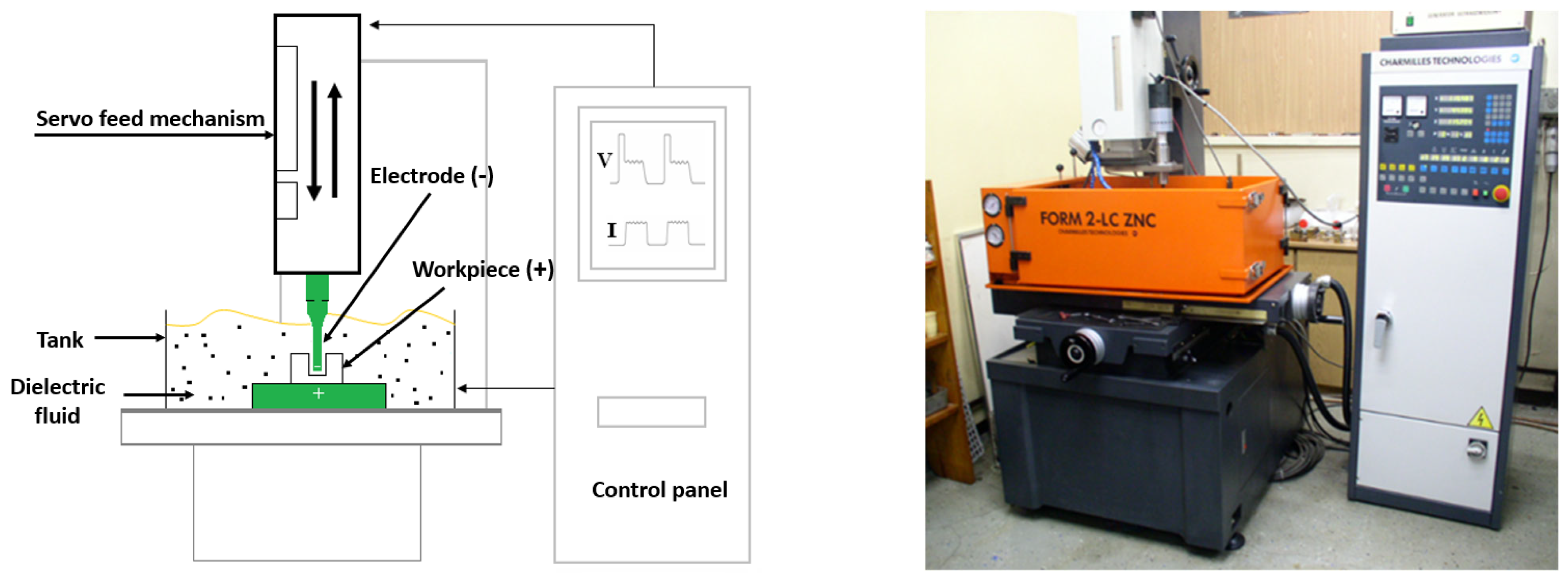
The experimental studies were conducted using the EDM machine Charmilles Form 2LC ZNC manufactured by AGIE CHARMILLES, which is located in Geneva, Switzerland. The EDM machine and the schematic of the process are shown in Figure 1. Electrolytic copper with a cross section of 8 × 5 mm and a length of 70 mm was used for this study, and kerosene Fluxelf2 was allowed to flow as the working fluid with a resistivity of 7.4 × 1010 Ω cm.

The experimental investigations were performed at a constant voltage (U = 50 V) and within different pulse current (I = 4–16 A), pulse duration (T_on = 75–200 μs), and pulse-off time (T_off = 18–75 μs) ranges, which are illustrated in

Table 2. Process parameters and their levels.

		Levels
Factor Symbol	Parameter	Low	High
I	Peak current [A]	4	16
Ton	Pulse-on time [µs]	75	200
Toff	Pulse-off time [µs]	18	75

. In each experiment, the pulse polarity was positive. The pulse current and pulse duration ranges in the selected experiment design were established based on prior preliminary tests and a review of the relevant literature, and the investigation parameters were the roughing, semi-finishing, and finishing values. The experimental layout was developed in accordance with Hartley’s experimental plan [17], the levels of which were defined to evaluate the influence of the pulse current, pulse duration, and pulse-off time on the MRR and Sa surface parameters, which reduced the number of machining runs required to obtain a statistically adequate result. No replications were performed in this study. The experimental work was designed to collect as much data as possible under varying EDM settings to ensure sufficient coverage for effective ML model training. A detailed analysis of the EDM process itself, including feature-level investigation, is beyond the scope of this work. Our main contribution lies in developing accurate ML models to predict the MRR and Sa, as well as proposing an inverse model for practical applications.

The design matrix and results are presented in

Table 3. Design matrix and results.

	Coded Factors			Response Variables
				S355 Alloy Steel		X5CrNi18-10 Stainless Steel		42CrMo4 Alloy Steel
Run	I	Ton	Toff	MRR [mm3/min]	Sa [μm]	MRR [mm3/min]	Sa [μm]	MRR [mm3/min]	Sa [μm]
1	16	200	50	21.13	17.4	20.70	18.7	21.88	14.4
2	16	100	25	22.18	9.19	20.29	13.6	22.53	20.8
3	14	200	50	22.91	12.8	17.84	11.5	23.63	27.6
4	14	150	36	20.71	10.5	19.70	12	21.95	25.2
5	14	100	25	19.37	9.42	19.16	11.1	20.74	20.9
6	14	75	18	18.64	21.4	17.81	10.4	19.36	12.7
7	12	200	50	22.01	29	19.29	12.8	21.70	19
8	12	150	36	20.76	23.8	19.23	12.3	20.15	26.5
9	12	100	25	19.45	17.9	18.25	12.7	20.14	29.3
10	12	75	18	18.14	13.2	15.90	11.9	18.29	18.1
11	10	200	50	19.10	16.8	16.32	14.6	19.90	17.9
12	10	150	36	19.11	21.4	16.68	14.5	20.15	20.9
13	10	100	25	16.86	14	15.30	11.9	16.87	9.14
14	10	75	18	16.24	7.92	14.49	14.2	17.08	9.53
15	8	200	75	12.64	11.1	10.32	8.3	16.45	9.74
16	8	150	50	13.87	7.76	12.06	8.81	14.74	10.6
17	8	100	36	13.20	7.78	10.96	8.61	13.79	9.42
18	8	75	25	14.16	6.6	11.92	9.29	15.60	9.11
19	6	200	75	6.97	7.55	8.43	9.32	7.99	8.62
20	6	150	36	9.89	8.88	9.55	7.96	11.48	11.2
21	6	100	36	11.01	8.28	9.23	8.51	12.72	9.46
22	6	75	25	7.83	13.7	6.17	6.13	9.07	8.77
23	4	100	25	2.82	5.86	2.88	7.35	3.31	8.39
24	4	75	25	2.39	8.34	2.40	6.55	2.92	7.26

. The assessment of the surface topography after the EDM was conducted using a Taylor–Hobson Form Talysurf Series 2 scan profilometer manufactured by Taylor–Hobson, which is located in Leicester, England, as shown in Figure 2. The area of each sample was measured at 6 × 4 mm, and the discretization interval for the X- and Y-axes was 10 µm.

The Sa parameter was chosen to characterize the surfaces in the electrical discharge machining. The Sa (arithmetic mean height) represents a three-dimensional parameter that is the average height deviation from the mean plane. The 2D roughness profile parameter (Ra) corresponds to the Sa parameter. The values can be computed by summing the heights and dividing the sum by the number of data points in the matrix without sign information. If M is the number of profile points, N is the number of profiles, X, Y, and Z are the heights of the profile at a given point, and the Sa can be computed using Equation (1) [18]:

$$S_a={\displaystyle \frac{a}{NM}}\sum _{x=0}^{N=1}{\sum }_{y=0}^{M=1}\left|z_{x,y}\right|$$

(1)

The material removal rate is determined by the amount of material removed from the workpiece per unit time of machining using Equation (2) [18]:

$$MRR={\displaystyle \frac{m_1-m_2}{\rho ∆t}}, \left[{\displaystyle \frac{{mm}^3}{min}}\right]$$

(2)

where m₁ is the sample weight before the process, m₂ is the sample weight after the process, ρ is the specific density, and t is the machining time, which was 5 min.

Each sample was weighed before manufacturing using a precision electronic digital balance (model: Radwag WPS 50/C/2) manufactured by Radwag, which is located in Radom, Poland, with a precision of 0.0001 g. The samples went through cleansing with compressed air after the EDM process and were subsequently reweighed.

3. Machine Learning Implementation

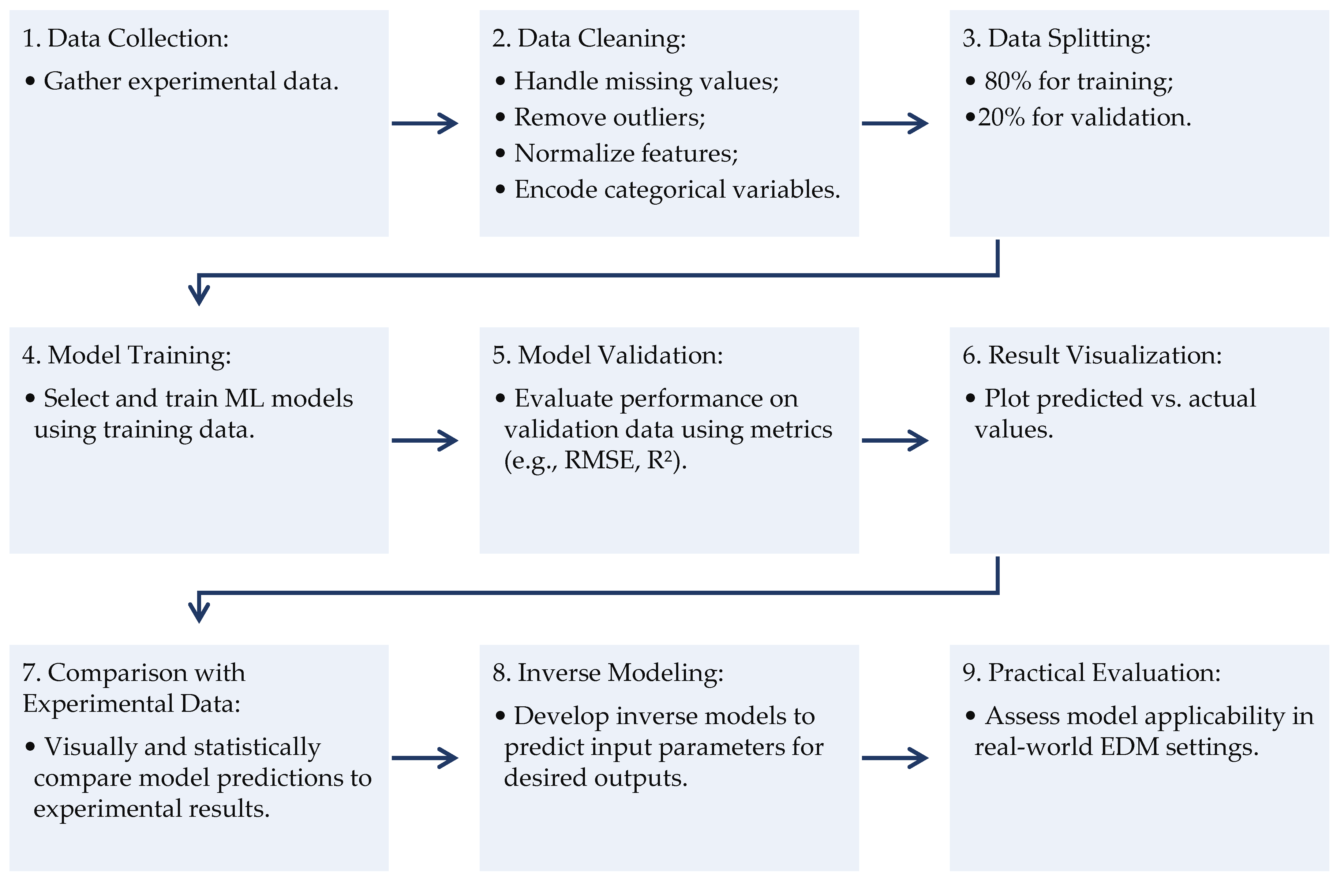
The experimental results from the experimental layout were utilized as a dataset in machine learning to predict the material removal rate and surface parameter (Sa). The work began by conducting extensive experimental work to collect the data from the experiments, which was then split into training (80% of the collected data) and validation (20% of the collected data) data.

The dataset is small, with only 72 training samples collected from three experiment plans. This constraint is due to the experimental nature of the EDM process, which is time-consuming. Regardless of the restricted sample size, several precautions to ensure the robustness and validity of the developed models have been taken. The DOE plan was used to have the best combination between factors with minimum experimental runs. The data were also split properly so that unseen data was always retained for testing to evaluate generalization and overfitting. Validation is performed on a 20% dataset, and similar performance was observed between both seen and unseen data. In general, the purpose of the study is to compare the performances of various ML models for the EDM process, focusing on which one could be more promising. This comparative reason is still applicable, even with a relatively small dataset.

In this study, the following ML techniques were employed to examine the best prediction technique for achieving the best ML model to predict the maximum material removal rate and minimum surface roughness for the EDM process: feedforward artificial neural network (FNN), support vector regression (SVR), decision tree regression (DTR), k-nearest neighbor (KNN) regression, random forest regression (RFR), and Gaussian process regression (GPR). The rationale for selecting these models was to evaluate the performance of the available models in modeling the EDM process.

Technically, the GPR and SVR models were expected to excel in this study because they are capable of handling complex and nonlinear models with small and noisy datasets. SVR is employed in the energy sector and shows an excellent performance in modeling nonlinear relationships and complex models [18,19]. Shi et al. [20] employed different ML models and reported the superiority of the GPR model over other ML models in terms of the prediction accuracy. Figure 3 shows the proposed flowchart of the ML implementation from the early stages and data collection to the creation of the final models and practical evaluation.

MATLAB Version R2021 was employed for developing these ML models, and the search gradient was employed to tune their hyperparameters. In this work, two performance metrics were utilized to evaluate the models: the root-mean-squared error (RMSE) and R-squared (R²) to assess the predictive accuracy and approximate actual outcomes.

4. Results and Discussion

In this study, we considered three factors: the EDM peak current, pulse-on time, and pulse-off time for three different materials. Two responses, the MRR and Sa, were measured across all the materials. In general, materials A (42CrMo4) and B (S355) had the highest MRRs, while material C (X5CrNi18-10) exhibited a minimal MRR under various combinations of factors, as depicted in Figure 4, which can be attributed to the nature of the material.

The thermal conductivity values at room temperature were as follows: 42CrMo4 alloy steel (material A): approximately 40 W/m·K; S355 alloy steel (material B): typically around 50 W/m·K; X5CrNi18-10 stainless steel (material C): usually around 15 W/m·K.

High thermal conductivity supports heat dissipation, which has an effect on the MRR and surface roughness in EDM.

As shown in Figure 4, the X5CrNi18-10 stainless steel (material C) with lower thermal conductivity had the lowest material removal rate, even with a larger peak current of 16 A. In general, this material absorbs less heat during machining, leading to lower material removal rates, as the heat generated in the EDM process is quickly dissipated [21]. The MRR can be further reduced due to less efficient melting and vaporization, but the electrical discharges may not provide enough power to maintain the material at the right temperature for efficient removal [22]. Additionally, the 42CrMo4 and S355 alloy steels showed similar material removal rates caused by their similar thermal conductivities. The specific electrical properties of materials play a critical role in the EDM performance; for example, the interaction between the thermal conductivity and discharge current is crucial.

The impacts of the process parameters on the surface parameter (Sa) are also shown in Figure 4. The lowest values were obtained for the S355 alloy steel (material B) and X5CrNi18-10 stainless steel (material C). The similarity in their Sa values even with different pulse-on times and its impact on the optimum parameters is a subject for further investigation. A higher parameter value was achieved for the 42CrMo4 alloy steel (material A).

In general, the surface roughness is inversely related to the thermal conductivity; lower peak currents generally yield better surface finishes, but at the cost of reduced MRRs. According to the experimental results, the optimal surface quality was achieved at lower currents with specific thermal conductivities, highlighting the trade-off between the MRR and surface quality. The 42CrMo4 alloy steel (material A) exhibited high hardness and strength [21,22,23,24]. In machine operations such as EDM, the greater the hardness of the material, the more challenging it becomes to achieve a smooth surface finish, resulting in increased surface roughness [21,22,23,24]. Graphite powder was recently added to kerosene-based dielectric fluid to enhance the EDM process [25].

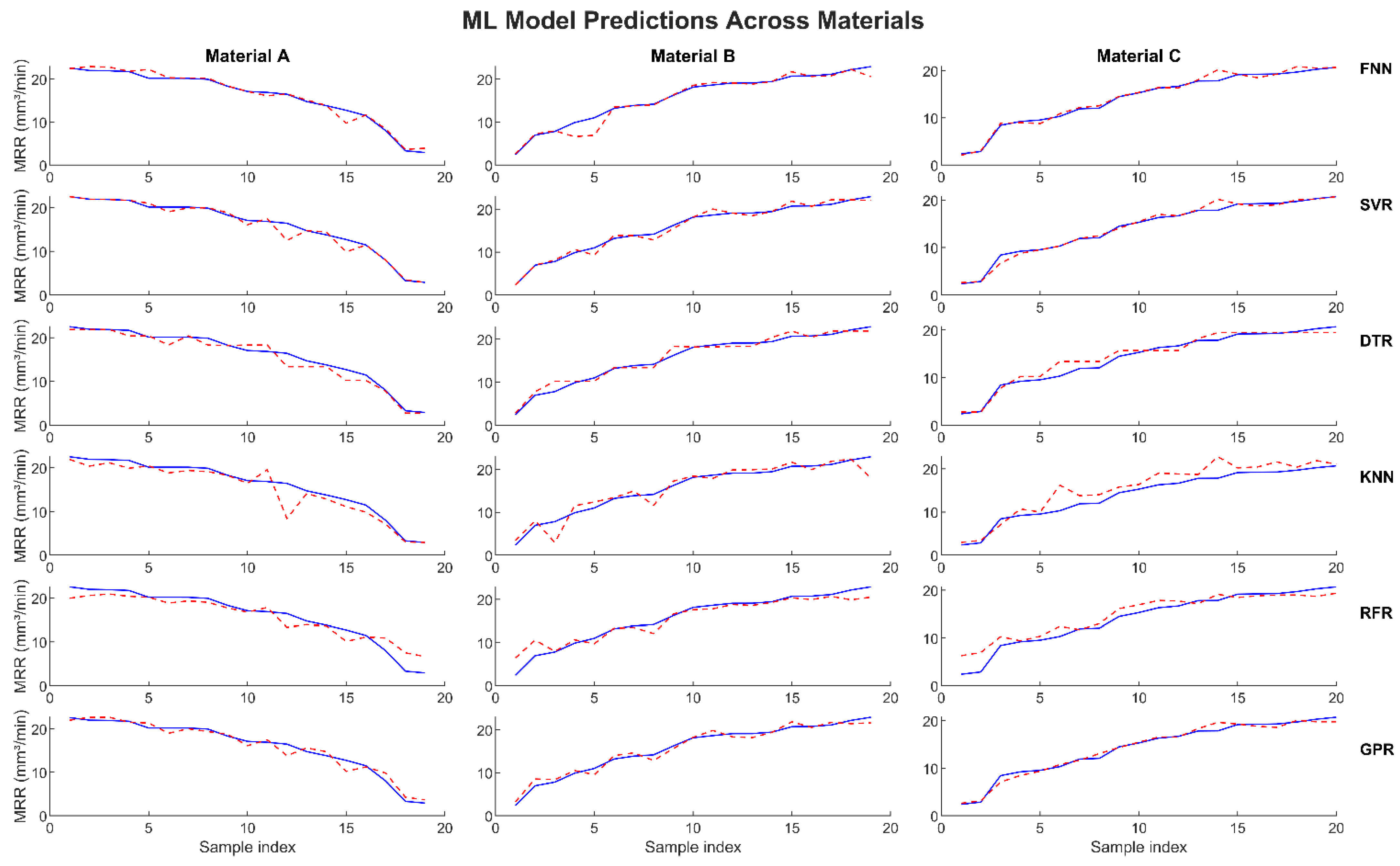
Figure 5 shows the MRR training results. The experimental data is shown as continuous blue lines, and the predicted data is represented by dashed red lines. As discussed earlier, 80% of the data (76 samples) were employed to train the developed ML models. In general, all the models showed similar trends to the experimental data. The GPR model demonstrated an excellent correlation with the experimental data across all the materials, while the KNN model exhibited some deviation at a high sample index, which could be because of its sensitivity to local noise, such that the presence of noisy data in the local neighborhood may lead to deviations in the predictions.

The first 19 samples represent material A. The DTR, KNN, and RFR models showed some deviation, while the rest of the models were in excellent correlation with the experimental data. Similar results are reported for the second and third 19 samples, which represent materials B and C, respectively, while the remaining 19 samples stand for material D. There was a large deviation using the KNN model and a small deviation using the RFR model.

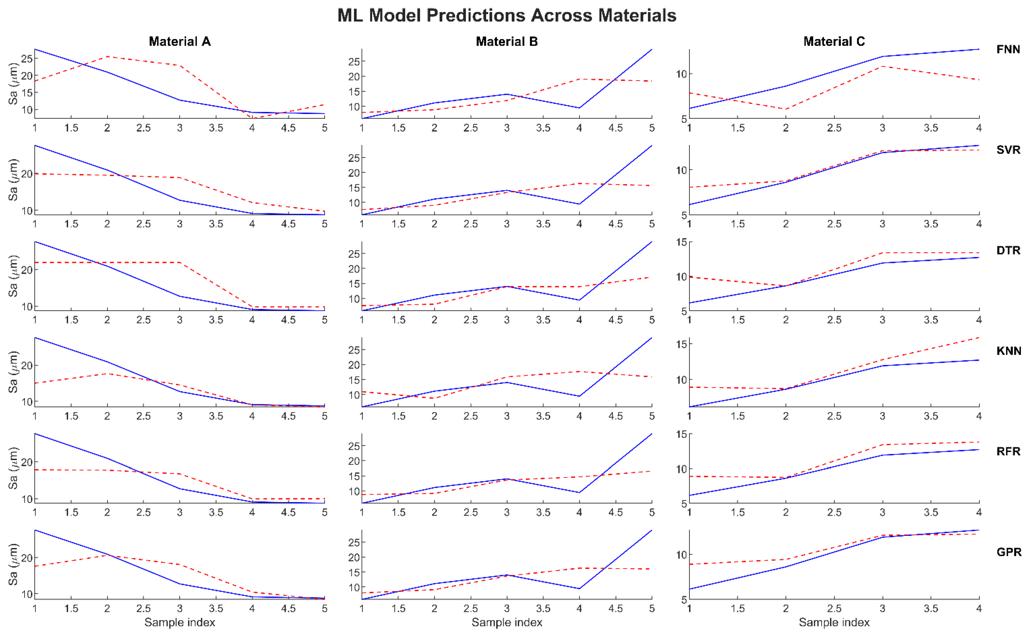
The ML models were then tested on unseen data. Figure 6 shows the ML model prediction data vs. new experimental data. A total of 19 samples representing 20% of the original dataset were employed as unseen data. We used unseen data for two reasons: (1) to validate and test the developed models on data that were not used for training them in order to prove their quality, and (2) to judge whether overfitting occurred, as similar performance on unseen data indicated no overfitting and good generalization of the model. The GPR model outperformed the other models, followed by the SVR and DTR models. The KNN model showed deviation across all the materials, even though a favorable correlation was reported for materials A, B, and C during the training phase. On the contrary, the FNN and RFR models showed some deviation for unseen data during the training phase, even though a good prediction was reported.

Figure 7 shows the surface roughness parameter (Sa) results of the training phase. Based on the results, the GPR model was the best predictor, followed by the SVR model; these results were similar to the findings reported for the MRR. The KNN model showed the poorest ability to predict the Sa across all the materials, while the RFR model showed some deviation, especially for materials A and C.

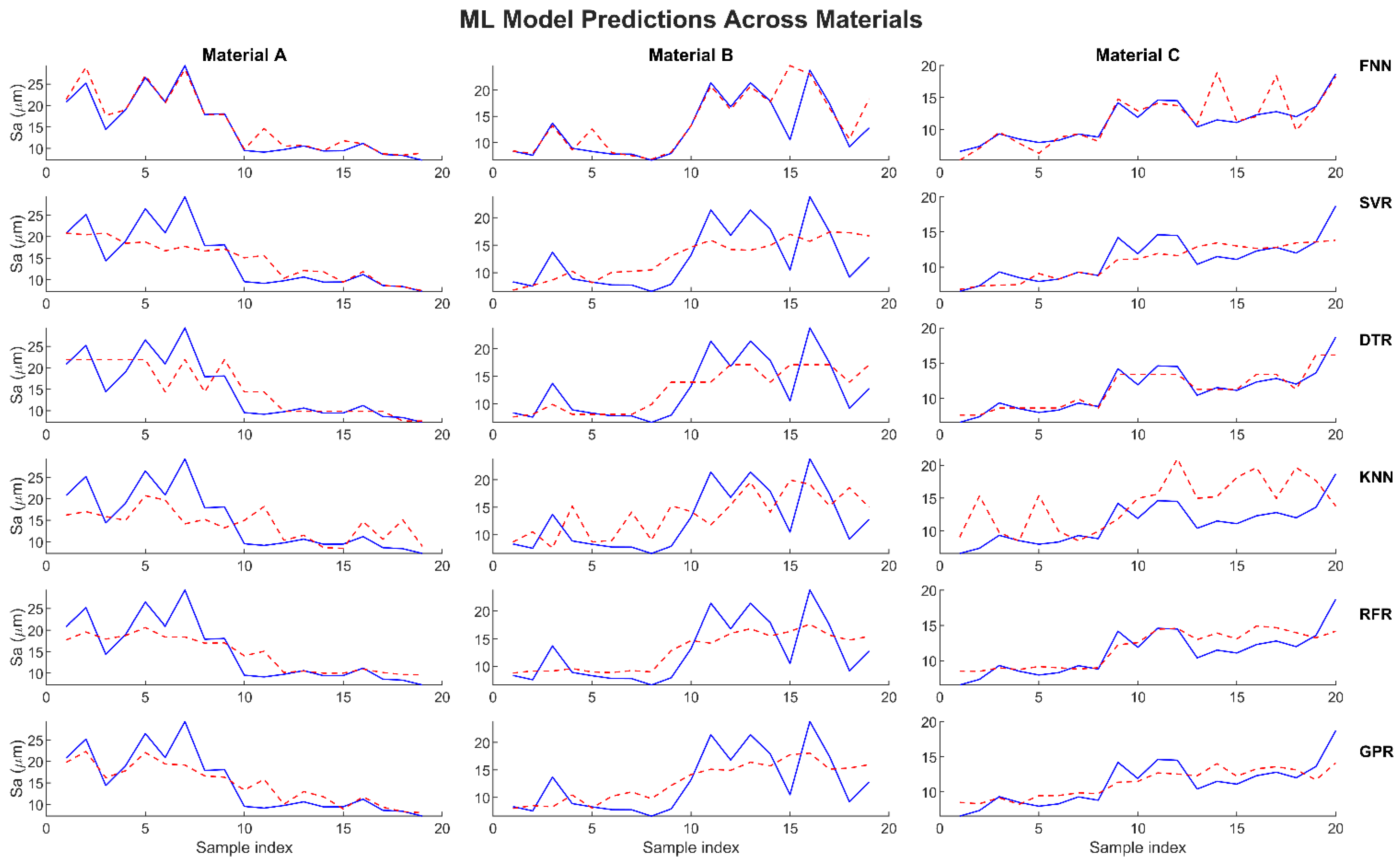
Similarly, the proposed models were tested for Sa in unseen data. Figure 8 shows the model predictions for the unseen experimental data. For all three materials, the GPR model was superior to the other models, and the SVR and DTR models were the second and third best models, respectively. The KNN model, however, showed a significant deviation across all the materials, while the RFR model only showed deviation for materials A and B. The FNN model showed a favorable prediction for material C and some deviation for materials A and B.

The results reported in Figure 6 and Figure 8 for unseen data suggest the validity of the models, in particular the GPR and SVR models, for use as reference models for studying the EDM process and its parameters.

It is worth mentioning that a grid search method was employed in this research work to optimize the hyperparameters for SVR and GPR. For the SVR, the following hyperparameters were searched: C_values (logspace (−3, 3, 5), Epsilon_values ([0.01, 0.1, 1]), and Gamma_values (logspace (−3, 2, 5)). On the other hand, the GPR kernel parameters, e.g., length scale and signal variance, and noise level, were optimized using the built-in automatic optimizer in MATLAB (fitrgp), which performs marginal likelihood maximization.

5. Evaluation of Predictive Model Effectiveness

The performance of the proposed ML models in terms of RMSE and R² was analyzed in this work. These characteristics are important for improving machining performance, for example, by predicting the surface roughness and material removal rates. The RMSE is used to measure the discrepancies between predicted and actual values, offering a straightforward indicator of the model accuracy and quantifying the model error. Meanwhile, R² indicates the percentage of variance in the dependent variable that can be described by the independent variables in the model and evaluates the goodness-of-fit [26,27].

The RMSE is essential in hyperparameter tuning and model selection and, at the same time, provides a quantitative measure to compare different models or configurations, confirming that the selected model generalizes well to unseen data [28,29,30]. Figure 9 shows the RMSEs for the training and validation data for both the MRR and Sa; similar results are listed in

Table 4. RMSE values across all materials and models of MRR datasets.

		FNN	SVR	DTR	KNN	RFR	GPR
Material A	Training	2.4689	1.2041	1.2764	2.1685	1.9472	1.1599
	Validation	3.2895	1.3959	1.5429	1.1475	2.0350	1.2285
Material B	Training	2.1517	0.7766	0.9787	1.8982	1.5277	0.9242
	Validation	2.2595	1.1076	1.5260	1.6837	2.1523	1.0672
Material C	Training	1.8071	0.6774	1.0872	2.2240	1.6159	0.6861
	Validation	1.4527	1.1760	2.7087	1.8661	1.3885	1.1740
Average	Training	2.1426	0.8860	1.1141	2.0969	1.6969	0.9234
	Validation	2.3339	1.2265	1.9259	1.5658	1.8586	1.1566

and

Table 5. RMSE values across all materials and models of Sa datasets.

		FNN	SVR	DTR	KNN	RFR	GPR
Material A	Training	2.6882	4.3676	3.8252	5.5224	3.7983	3.3698
	Validation	5.9677	4.6807	4.8951	5.8683	4.9519	5.1194
Material B	Training	5.0556	4.4135	3.8620	5.1707	3.6470	3.9045
	Validation	9.2359	6.8596	5.8948	7.4231	6.3231	6.7015
Material C	Training	2.0446	1.8687	1.0952	4.6365	1.7938	1.7905
	Validation	1.8833	1.0148	2.0375	2.1471	1.6853	1.4642
Average	Training	3.2628	3.5499	2.9275	5.1100	3.0797	3.0216
	Validation	5.6956	4.1850	4.2758	5.1462	4.3201	4.4284

for the MRR and Sa, respectively.

The GPR and SVR models outperformed the other models in terms of the MRR, with the average RMSE values of the three materials equal to 0.9234 and 0.8860, respectively, for the training data, and equal to 1.1566 and 1.2265, respectively, for the validation data. The FNN model showed the worst performance during the training and validation phases. Regarding the Sa, the GPR and DTR models showed the minimum Sa values for the training data, while the SVR and DTR models showed the minimum Sa values for the validation data. In general, the developed ML models predicted the Sa with an RMSE of 4.1850 (the SVR model for the validation data), which subsequently represents more than a 10% deviation from the actual Sa value, highlighting the need to conduct more extensive experimental work to obtain more data for training/validation.

Figure 10 shows a bar chart of the R² values across the proposed materials and models, and the same results are listed in

Table 6. R² values across all materials and models of MRR datasets.

		FNN	SVR	DTR	KNN	RFR	GPR
Material A	Training	0.9135	0.9676	0.9526	0.8632	0.8907	0.9609
	Validation	0.8922	0.9564	0.9056	0.9478	0.8184	0.9401
Material B	Training	0.8629	0.9766	0.9701	0.8876	0.9232	0.9734
	Validation	0.8461	0.9796	0.9483	0.9371	0.8946	0.9747
Material C	Training	0.8581	0.9804	0.9603	0.8339	0.9089	0.9842
	Validation	0.8365	0.9253	0.6613	0.8393	0.9234	0.9364
Average	Training	0.8782	0.9749	0.9610	0.8616	0.9076	0.9728
	Validation	0.8583	0.9538	0.8384	0.9081	0.8788	0.9504

. The achieved R² values (i.e., the MRR training dataset) for both the GPR and SVR models are more than 0.97, indicating that the model discovered around 97% of the total variation in the observed Sa values for materials A, B, and C.

Following the surface roughness (Sa) prediction, the DTR model outperformed the other models during the training phase, as shown in

Table 7. R² values across all materials and models of Sa datasets.

		FNN	SVR	DTR	KNN	RFR	GPR
Material A	Training	0.8071	0.5860	0.6824	0.3381	0.6683	0.7536
	Validation	0.0777	0.5928	0.5547	0.3600	0.5372	0.5129
Material B	Training	0.7647	0.3237	0.4822	0.0718	0.5334	0.4707
	Validation	−0.1939	0.2661	0.4580	0.1406	0.3894	0.2995
Material C	Training	0.5179	0.5999	0.8626	−1.4627	0.6354	0.6327
	Validation	0.5440	0.8513	0.4005	0.3343	0.6103	0.6904
Average	Training	-	0.5032	0.6757	-	0.6124	0.6190
	Validation	-	0.5701	0.4711	-	0.5123	0.5009

; however, it showed the lowest R² for the validation/unseen data, with the R² equal to only 0.4711. The GPR and RFR models showed similar R² values for the training and validation data: about 0.61 and 0.51, respectively. The FNN and KNN models showed negative values for some materials, which indicates the unsuitability of these models to Sa prediction in EDM processes.

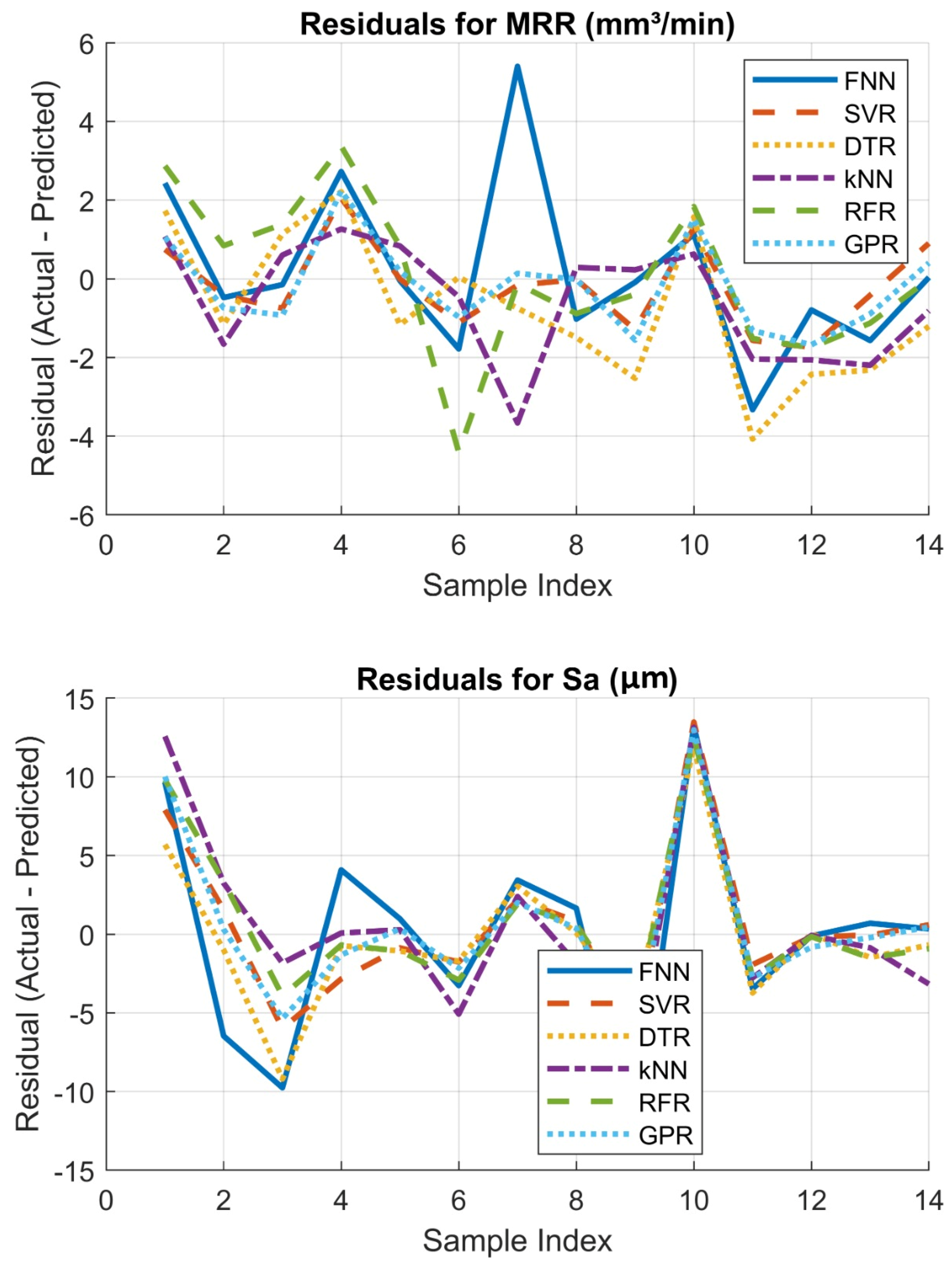
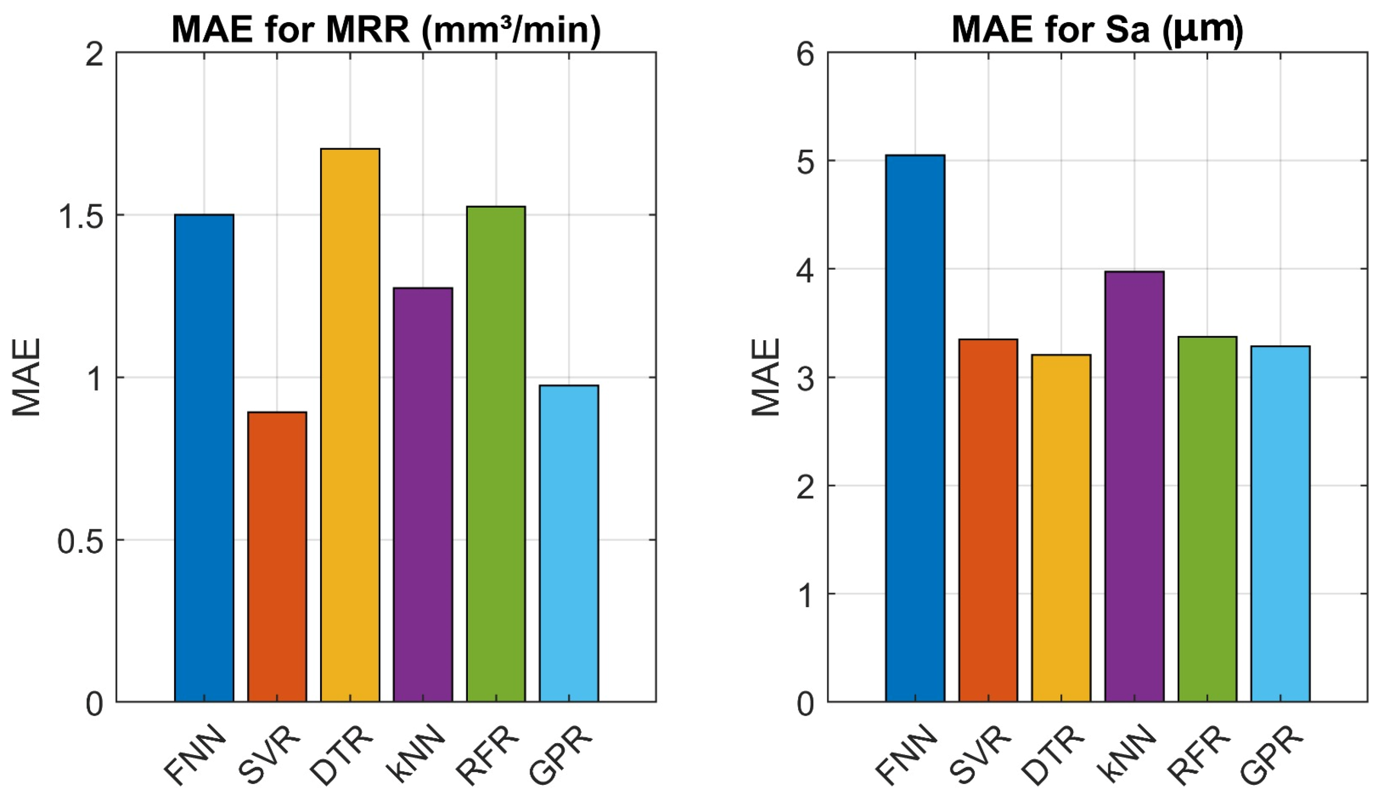
Figure 11 shows the residual plots for the predicted outputs (MRR and Sa) across all the materials using the validation dataset, revealing the validity of the GPR and SVR models with low residuals across the three materials considered, which can also be seen in Figure 12, where the MAEs are shown for all the ML models.

6. Practical Implications

This study demonstrated that the SVR and GPR models outperformed the other models in terms of seen and unseen data; in particular, the developed models connected the EDM setting with the MRR and surface roughness for three different materials. These findings can be applied in industries where the EDM setting is often used to predict the performance of the EDM process without the need to conduct any experimental work. For instance, once the EDM setting is initialized, the MRR and Sa will be known at the very beginning. Another potential practical implication is the development of inverse GPR and SVR models and their subsequent employment to determine the EDM setting based on the desired material, MRR, and Sa.

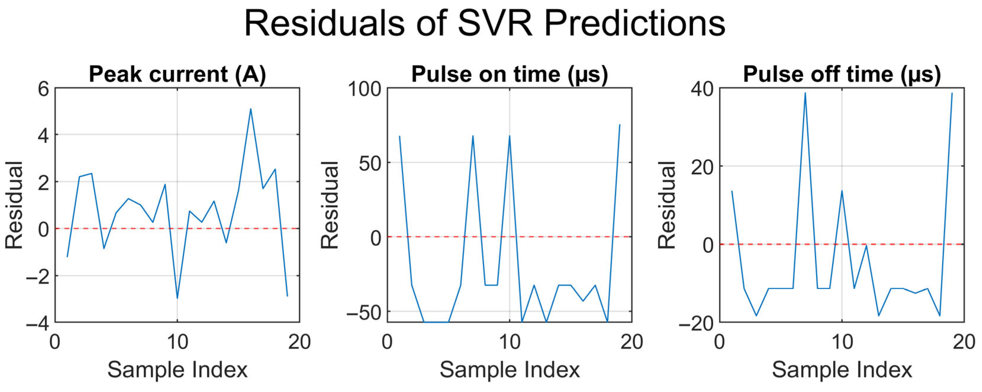
An inverse model was developed further to investigate the possibility of predicting the EDM setting per given MRR and Sa. An SVR model was developed considering the following inputs: the material, MRR, and Sa, with the peak current, pulse-on time, and pulse-off time as the outputs. The data were again divided into training data (seen data) (80%) and validation data (unseen data) (20%).

The results of the EDM setting prediction utilizing unseen data are summarized in Figure 13. Valuable predictions were demonstrated for the three materials, with better predictions for the pulse-on time, and moderate predictions for both the pulse-off time and peak current. In general, these results can be integrated with the EDM controller for real-time decision making to determine the MRR and Sa.

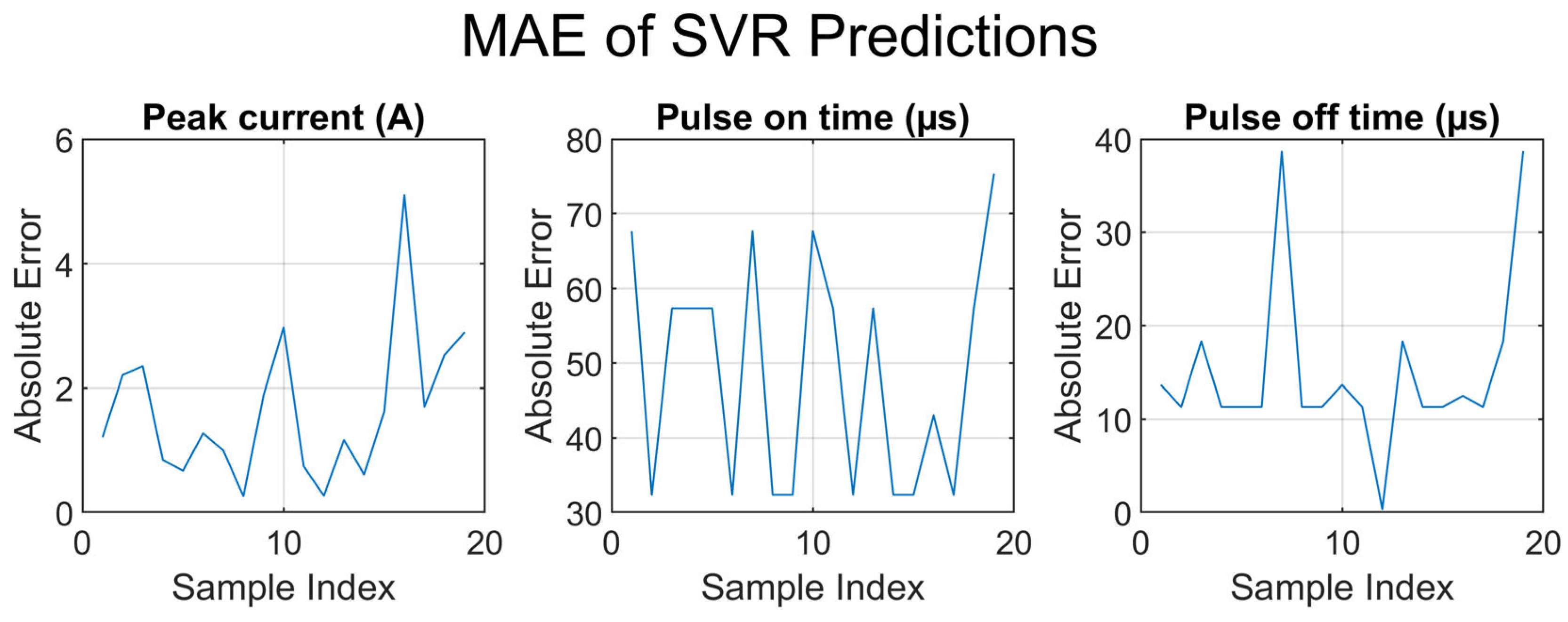
Figure 14 and Figure 15 show the MAE and residual plots of the unseen dataset of the proposed inverse model. Figure 14 shows the MAEs of the peak current, pulse-on time, and pulse-off time of the inverse model in detail. Clearly, the prediction was more accurate for the pulse-on time, followed by those for the pulse-off time and peak current. A similar trend is shown in Figure 15, where the residuals are plotted for the aforementioned outputs. These results highlight the validity of the future implementation of the proposed inverse model in EDM processes in scenarios where the target MRR and Sa values are specified, allowing the EDM system to automatically select and implement the optimal process parameters.

7. Conclusions

In this study, we developed different ML models of the EDM process under a wide range of machine settings (i.e., the peak current, pulse-on time, and pulse-off time) and materials (i.e., two types of alloy steels and a stainless steel). In addition, two outputs were considered: the material removal rate (MRR) and surface roughness (Sa). According to the results, the GPR model outperformed the other ML models in terms of the RMSE and R², followed by the SVR model. The average RMSE values of the GPR model across the different materials were 0.9234 and 3.0216 for the MRR and Sa, respectively. Similarly, the R² values were 0.9728 and 0.6190 for the MRR and Sa of the GPR model, respectively. In contrast, the KNN and FNN models showed the worst performance, which could be attributed to their sensitivity to local noise in data. The proposed ML models were able to accurately predict the EDM response, indicating that they can be used to model and simulate EDM machine predictions. In future work, the authors plan to combine the ML strategies with the additional study of the structures of materials before and after the EDM process, as well as the prediction of the effects of the parameters on a larger range of material responses. This study enhances the existing literature in the context of EDM process modeling, providing insight into EDM process optimization in industrial applications. Future work will focus on implementing an inverse model for the real-time EDM process, enabling users to specify their desired MRR and Sa values, upon which the system will automatically determine the appropriate machining settings.