Optimization of Process Parameters for Advanced High-Strength Steel JSC980Y Automotive Part Using Finite Element Simulation and Deep Neural Network

Abstract

In the stamping process of automotive parts, springback is a major problem when using Advanced High-Strength Steel (AHSS). This phenomenon significantly impacts the shape accuracy of products and is difficult to control. This study aims to optimize process parameters such as blank holder force (BHF), die clearance, and blank width to minimize springback in the workpiece. Using optimal process parameters will enhance the efficiency of die compensation processes. The study uses the Finite Element Method (FEM) simulation to predict forming behavior. The case study, Reinforcement-CTR PLR, is made from AHSS grade JSC980Y with a thickness of 1 mm. Four material model combinations were evaluated against actual experiment results to select the most accurate springback prediction model. A full factorial design was used for experiments with varied process parameters. The optimization process used regression and various Artificial Neural Networks (ANNs). From the result, a Deep Neural Network (DNN) with two hidden layers performed with the highest accuracy compared to the other models. The optimal process parameters were identified as 27.62 tons BHF, 1 mm die clearance, and a 290 mm blank width. These optimal results achieved 98.05% of the part area within a displacement tolerance of −1 to 1 mm, closely matching FEM-based validation.

1. Introduction

The automotive industry faces new challenges, especially with the use of lightweight and higher strength materials such as high-strength steel, carbon fiber composites, and alloys. These materials have significant advantages in terms of fuel efficiency, environmental impact, and passenger safety [1]. Advanced High-Strength Steel (AHSS) is a popular material in automotive body structure production due to its low cost and high strength-to-elastic modulus ratio compared to other materials. However, the AHSS forming process is likely to encounter problems, such as fracture, wrinkling, and springback. Springback is a more significant issue in the AHSS forming process compared to conventional steels. This problem is the distortion of part dimensions that deviate from the desired shape and affects assembly processes. It is caused by elastic regions inside the material that are not fully transformed into plastic regions and try to return to their original shape after forming. Many researchers and engineers are trying to solve this problem by using Finite Element Method (FEM) simulations for experimental analysis. For example, one approach involves using a counter punch with end gaps to create spring-go, which compensates for the springback effect [2]. Another method uses adjustable blank holder forces during the forming process [3]. A third technique is two-step forming, where the single upper die is separated into a pad at the top of the workpiece, and forming occurs in the final step [4]. On the other hand, the automotive parts often have complex geometries. Hence, a die compensation method has to be used for solving this problem [5]. This method adjusts the die surface by using FEM analysis. The simulation replicates the forming process to identify shape distortions and compensates the die surface to achieve the desired workpiece shape. However, the process parameters used in forming must be optimized to minimize springback first for effective compensation [6]. In the engineering field, the design of experiments (DOE) and regression are widely used for optimizing the most suitable parameters [7]. The benefit of this method is not only optimizing the parameters but also reducing the time for various experiments. For instance, Özdemir [8] used the Taguchi method and response surface methodology (RSM) to optimize the parameters for reducing springback with only 16 experiments. Ingarao et al. [9] employed FEM and RSM to investigate the effect of friction and blank holder force on DP600 and DP1000 workpieces and parameters to minimize springback and thinning.

Currently, Artificial Intelligence (AI) [10] has gained in popularity and seen a significant increase in performance [11]. As a result, AI is increasingly used in several fields, including healthcare, education, language technology, economics, commerce, and industrial manufacturing [12]. The most popular algorithm is the Artificial Neural Network (ANN). ANN is a learning technique in the field of machine learning (ML) that mimics the human brain system’s learning process. In 2006, ANN gained popularity with the introduction of deep learning (DL) [13]. DL enhances ANN performance by using multiple hidden layers in the ANN model to train on complex data, especially in the manufacturing industry for analyzing defects in sheet metal forming, particularly the springback phenomenon [14,15,16]. A common and effective strategy in such research is to develop a highly accurate predictive model. This model aims to map the complex non-linear relationships between process inputs and the resulting manufacturing outcome. ANN and Deep Neural Network (DNN) are exceptionally suited for this predictive task due to their ability to learn intricate patterns from data generated by experiments or FEM simulations.

Once such an accurate model is established, it can then be leveraged by various optimization algorithms to identify the optimal process parameters. While other AI driven optimization techniques, such as Genetic Algorithms (GAs) [17] or Particle Swarm Optimization (PSO) [18], are powerful for searching large parameter spaces and have been effectively used with ANN models, the initial development of a robust predictive model is a critical foundational step. Similarly, reinforcement learning (RL) [19], another advanced AI technique, is typically more suited for sequential decision making or learning control policies in dynamic environments rather than for directly creating a static predictive map of the process parameters to springback. Therefore, for studies aiming to optimize processes based on accurate predictions, a strong focus on developing ANN/DNN-based models is a well-justified approach. Indeed, several studies have demonstrated the effectiveness of ANNs in springback analysis for solving or decreasing this problem. For instance, Spathopoulos and Stavroulakis [14] developed an ANN model to predict springback at different locations on a S-rail part. The model yielded results that showed good agreement with those obtained from the FEM simulation, particularly in predicting springback trends and magnitudes. Narayanasamy and Padmanabhan [15] compared the performance of regression and ANN models to predict springback angles. Their study showed that the ANN outperformed the regression model in terms of prediction accuracy. El Mrabti et al. [16] simulated a deep drawing process using FEM simulation and conducted DOE experiments to collect data to train an ANN model. After training the ANN model, PSO was used to optimize the process parameters. Finally, by using the optimized parameters, they found that springback was reduced significantly.

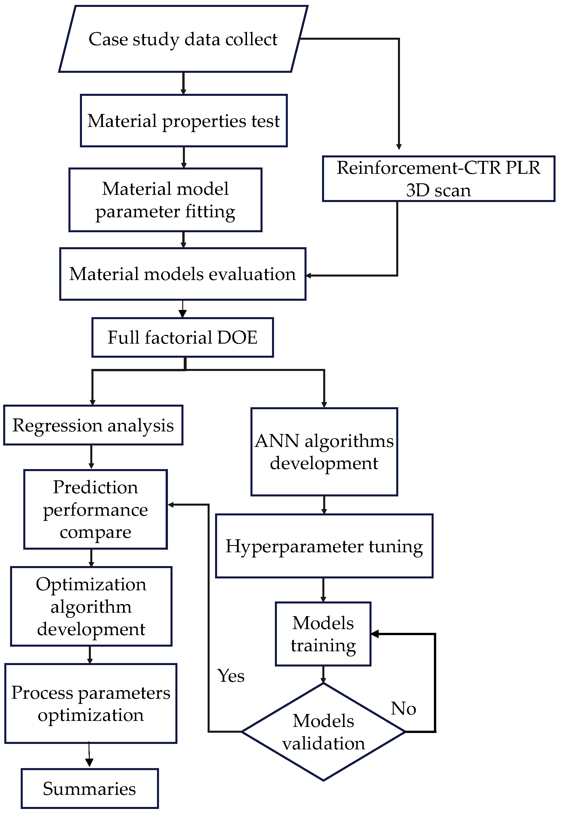
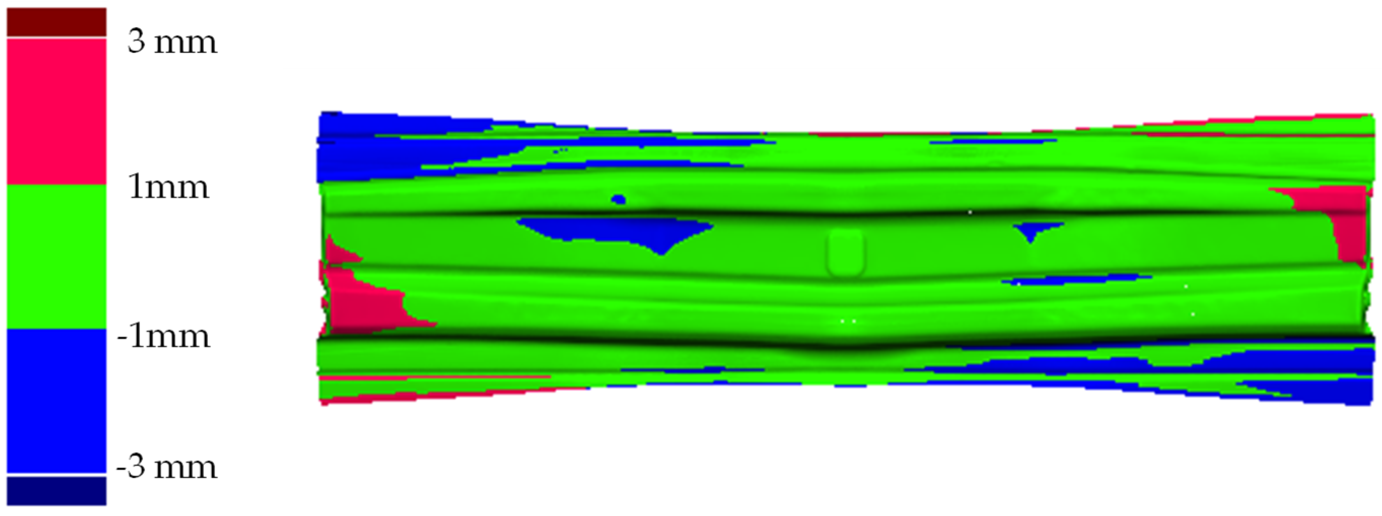
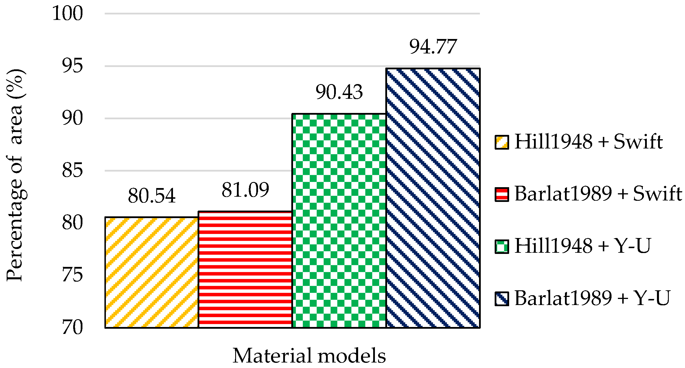
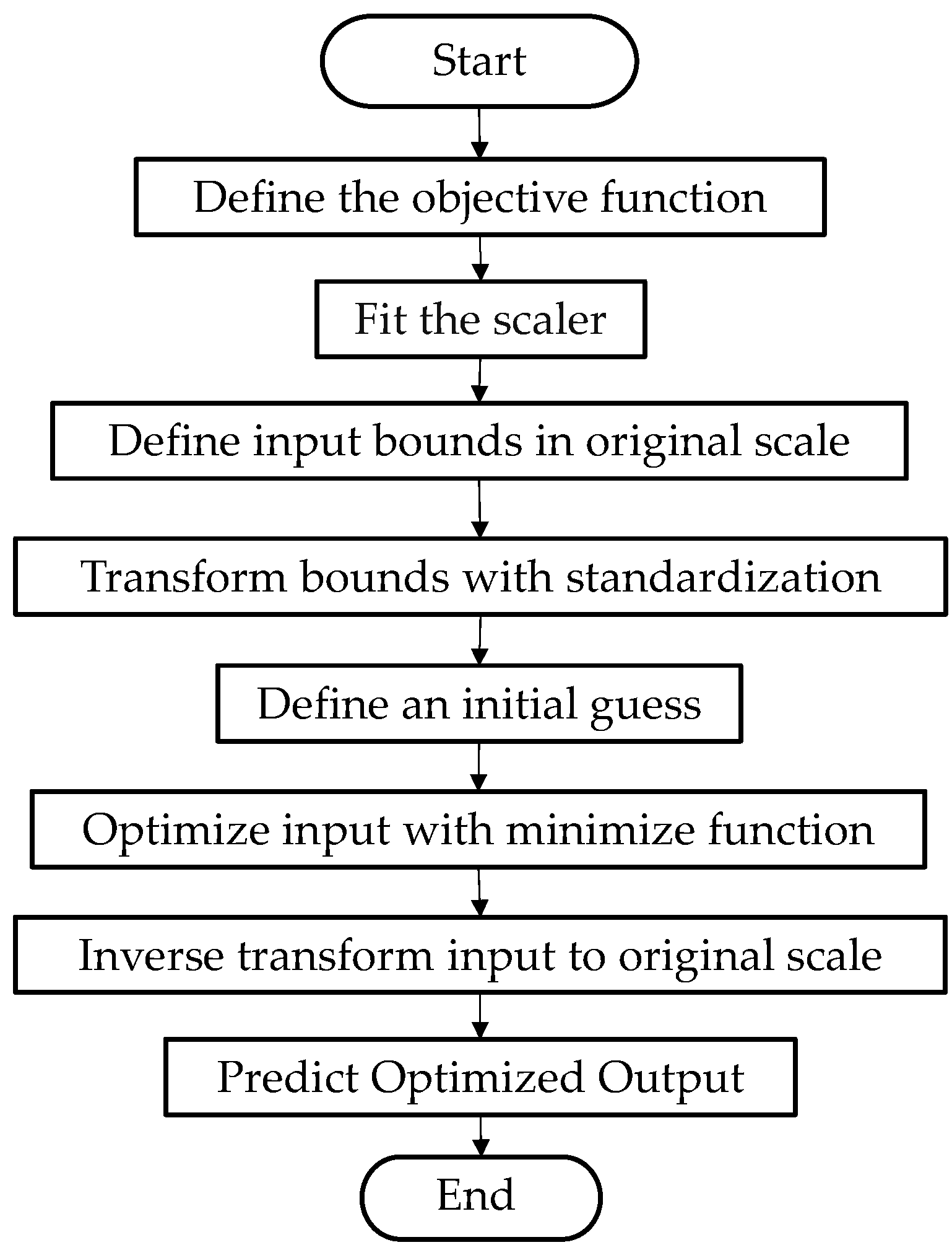
However, while FEM and traditional optimization methods are common, a comparison of various ANN architectures, particularly DNN with multiple hidden layers, for optimizing these process parameters to maximize the conforming area of a complex AHSS automotive part like the Reinforcement-CTR PLR remains an area requiring more detailed investigation. Specifically, the efficacy of different ANN complexities in capturing the springback behavior and their direct application to achieve strict dimensional tolerances over a large part area needs further exploration. Consequently, this research aims to use FEM simulation to predict the forming process of an industrial automotive part, the Reinforcement-CTR PLR. Four combinations of material models were compared in terms of prediction accuracy performance to select the most accurate springback prediction for use in optimization experiments. For the optimization experiments, a full factorial design was employed where three process parameters: blank holder force, die clearance, and blank width were varied. The springback result was obtained by measuring the percentage of area where the displacement between the predicted shape before and after springback occurred within the range of −1 to 1 mm. After the experiment, regression was used to create a prediction model. Meanwhile, different types of ANN algorithms were created and trained with data from simulation results, and all ANN models were compared to the regression model in terms of accuracy with data validation. The most accurate model was selected for use in optimizing the process parameters to minimize springback with an optimizing algorithm. Finally, the FEM simulation was conducted to verify the predicted result from the optimized procedure. For ease of understanding, the overall procedure workflow is shown in Figure 1.

2. Materials and Methods

2.1. Workpiece

The case study in this work is a component of a car structure’s B-Pillar “Reinforcement-CTR PLR” made from JSC980Y AHSS. The production process consists of five steps: drawing, trimming, CAM trimming, resting, and piercing. This study focuses only on the drawing process, as it is where springback occurs after forming. This process was conducted with a SIMPAC hydraulic press with a press capacity of 800 tons. Figure 2 depicts the automotive part Reinforcement-CTR PLR after the drawing process with the forming tools.

2.2. Material Properties and Testing

In this study, Finite Element simulation was used to investigate the springback of the Reinforcement-CTR PLR. The material model parameters were determined using data from uniaxial tensile testing and tension–compression testing.

2.2.1. Uniaxial Tensile Testing

In this work, uniaxial tensile testing was used to characterize the basic mechanical properties of the material with a universal testing machine, “INSTRON 8801”. The testing specimen was prepared according to a standard testing subsize shape, ASTM E8/E8M [20]. ARAMIS Digital Image Correlation (DIC) was used as the measurement tool to calculate the deformation. Three orientations related to the rolling direction (0°, 45°, and 90°) were investigated to capture the material properties in each direction with a crosshead velocity of 0.01 mm/s and a strain rate of 0.0002 s⁻¹. True stress–strain curves of JSC980Y AHSS obtained from uniaxial tensile tests at 0°, 45°, and 90° to the rolling direction, demonstrating the material’s anisotropic behavior, are presented in Figure 3. The main mechanical properties, including Young’s modulus (E), yield strength (YS), ultimate tensile strength (UTS), uniform elongation ${\epsilon }_u$, and r-value for each direction, are summarized in

Table 1. Mechanical properties of JSC980Y.

Directions	E (GPa)	YS (MPa)	UTS (MPa)	${\mathit{\epsilon }}_{\mathit{u}}$ (%)	r-Value
0°	189	589	946	9.78	0.81
45°	189	647	1073	10.39	0.79
90°	204	635	1036	10.04	0.84

.

2.2.2. Tension–Compression Testing

Tension–compression testing was used to determine the Yoshida–Uemori mixed kinematic hardening rule parameters. The testing specimen was prepared and tested according to the SEP1240 standard shape [21]. The cyclic loading test operates by applying tensile and compressive loads on a single axis to the specimen in cycles. In this work, the universal testing machine INSTRON 8801 was used to perform the cyclic testing. This testing was performed for only one cycle because of the limitations of the testing machine. This testing is essential for capturing the Bauschinger effect and predicting springback accurately [22]. A specimen fixture was used to avoid buckling during testing. To minimize the errors from friction, the contact surfaces between the specimen and the fixture were coated with a dry film lubricant. The fixture held the specimen using a coil spring force [23]. A DIC camera captured the local displacement of the specimen during testing. The obtained cyclic true stress–strain curve of JSC980Y AHSS from a single cycle tension–compression test that is used for calibrating the Yoshida–Uemori hardening model parameters is presented in Figure 4.

2.3. Material Models

In the initial stages of this work, a comparison of different material models was conducted with Finite Element simulation. A material model is a mathematical equation used to describe the behavior of a material under stresses and strains. The common model is divided into two parts. First, the yield criterion is a model that describes the behavior of a material under stress during elastic deformation. Second, the hardening model describes the behavior of a material after plastic deformation occurs. In this study, a total of four pairs of material models were compared.

2.3.1. Hill 1948 Yield Criterion

The anisotropic Hill 1948 yield criterion [24] is popular for use in simulating plastic deformation in anisotropic sheet metals. This model was developed based on the Huber–Mises–Hencky criterion [25] and used a quadratic equation to account for the material properties in each direction. This approach assumes that the material exhibits anisotropy with three orthogonal planes of symmetry. The equations of the Hill 1948 yield criterion model can be written as Equation (1):

$$\begin{array}{c}2f\left({\sigma }_{ij}\right)\equiv F{\left({\sigma }_{yy}-{\sigma }_{zz}\right)}^2+G{\left({\sigma }_{zz}-{\sigma }_{xx}\right)}^2+H{\left({\sigma }_{xx}-{\sigma }_{yy}\right)}^2+2L{{\sigma }^2}_{yz}+\\ 2M{{\sigma }^2}_{zx}+2N{{\sigma }^2}_{xy}=1\end{array}$$

(1)

where $f$ is the yield function, and the parameters $F$, $G$, $H$, $L$, $M$, and $N$ are material constants representing the state of anisotropy. $x,y,$ and $z$ correspond to the principal anisotropic axes. In the case of sheet metal forming, the $x$-axis aligns with the rolling direction, the $y$-axis aligns with the transverse direction, and the $z$-axis aligns with the thickness of the material. Under plane stress conditions $\left({\sigma }_{zz}={\sigma }_{zx}={\sigma }_{yz}=0\right),$ the equation can be expressed as Equation (2):

$$2f\left({\sigma }_{ij}\right)\equiv \left(G+H\right){{\sigma }^2}_{xx}-2H{\sigma }_{xx}{\sigma }_{yy}+\left(H+F\right){{\sigma }^2}_{yy}+N{{\sigma }^2}_{xy}=1$$

(2)

When using the Hill 1948 yield criterion in sheet-forming simulations, an r-value-based method was chosen to identify the yield criterion material parameters. Lankford coefficients $(r_0, r_{45,}$ and $r_{90})$ are used based on the relationship between the constants $F$, $G$, $H,$ and $N$. This relationship, derived from the flow rule, is presented in the following Equations (3)–(6):

$$F={\displaystyle \frac{r_0}{r_{90}(1+r_{90})}}$$

(3)

$$G={\displaystyle \frac{1}{(1+r_0)}}$$

(4)

$$H={\displaystyle \frac{r_0}{(1+r_0)}}$$

(5)

$$N={\displaystyle \frac{(r_0+r_{90})(1+2r_{45})}{2r_{90}(1+r_0)}}$$

(6)

In several simulation software programs, this model’s parameters can be determined using the simple testing results from uniaxial tensile testing and r-values in different directions. The material parameters of the Hill 1948 model used in this research were directly obtained from the material testing results presented in Table 1.

2.3.2. Barlat 1989 Yield Criterion

The non-quadratic Barlat–Lian 1989 yield criterion [26] is a non-orthogonal coordinate model that extends Hosford’s criterion [27] for enabling a more accurate description of material behavior under stress. In normal anisotropy form, this yield function is defined by specific coefficients in Equation (7):

$$f=a{\left|k_1+k_2\right|}^M+a{\left|k_1-k_2\right|}^M+c{\left|{2k}_2\right|}^M={2{\sigma }_e}^M$$

(7)

where $k_1$ and $k_2$ are given by Equations (8) and (9):

$$k_1={\displaystyle \frac{{\sigma }_{xx}+h{\sigma }_{yy}}{2}}$$

(8)

$$k_2=\sqrt{{\left({\displaystyle \frac{{\sigma }_{xx}-h{\sigma }_{yy}}{2}}\right)}^2+p^2{{\sigma }_{xy}}^2}$$

(9)

Material parameters $a$, $c$, $h$, and $p$ are identified by Equations (10)–(12):

$$a=2-c={\displaystyle \frac{2{\left(\frac{{\sigma }_e}{{\tau }_{s2}}\right)}^M-2{\left(1+\frac{{\sigma }_e}{{\sigma }_{90}}\right)}^M}{1+{\left(\frac{{\sigma }_e}{{\sigma }_{90}}\right)}^M-{\left(1+\frac{{\sigma }_e}{{\sigma }_{90}}\right)}^M}}$$

(10)

$$h={\displaystyle \frac{{\sigma }_e}{{\sigma }_{90}}}$$

(11)

$$p={{\displaystyle \frac{{\sigma }_e}{{\tau }_{s1}}}\left({\displaystyle \frac{2}{2a+2^{M}c}}\right)}^{{\displaystyle \frac{1}{M}}}$$

(12)

where ${\tau }_{s1}$ and ${\tau }_{s2}$ are the yield stresses in two different shear tests. While $M$= 6 for Body-Centered Cubic (BCC) materials and $M$ = 8 for Face-Centered Cubic (FCC) materials, an alternative, simpler procedure relies on r-values obtained through Equations (13) and (14):

$$a=2-c=2-2\sqrt{{\displaystyle \frac{r_0}{1+r_0}}.{\displaystyle \frac{r_{90}}{1+r_{90}}}}$$

(13)

$$h=\sqrt{{\displaystyle \frac{r_0}{1+r_0}}.{\displaystyle \frac{{1+r}_{90}}{r_{90}}}}$$

(14)

The Barlat 1989 yield criterion material parameters used in this study are summarized in

Table 2. Material parameters for Barlat 1989 yield criterion model.

$\mathit{a}$	$\mathit{c}$	$\mathit{h}$	$\mathit{p}$	$\mathit{M}$
1.09	0.91	0.98	0.96	6

. These parameters were calculated from the material testing results.

2.3.3. Swift Hardening Model

The Swift or Krupkowski hardening law is a non-linear hardening equation that is popularly used to describe the plastic behavior in sheet metal forming simulations. It is easy to use and has satisfactory simulation results. The hardening curve can be described by Equation (15) [28]:

$$\sigma =K{\left({\epsilon }_p+{\epsilon }_0\right)}^n$$

(15)

where $K$ is a material constant, ${\epsilon }_p$ is the plastic strain, ${\epsilon }_0$ is the offset true strain, and $n$ is the strain hardening exponent. The fitted material parameters of this model are listed in

Table 3. Material parameters for the Swift hardening model.

$\mathit{K}$	${\mathit{\epsilon }}_0$	$\mathit{n}$
1371.12	0.000638	0.1168

.

2.3.4. Yoshida–Uemori Hardening Model

The Yoshida–Uemori (Y–U) hardening model [22] was developed by Yoshida and Uemori by expanding the Chaboche model [29] to describe the cyclic deformation behavior of materials when experiencing large-strain cyclic plasticity with greater accuracy. This model is defined in two-surface frameworks with a yield surface and a bounding surface that can evolve in size and position. The yield surface is assumed to exhibit kinematic hardening, and the bounding surface is assumed to exhibit mixed isotropic–kinematic hardening. This allows the Y–U model to accurately capture the transient Bauschinger effect and some of the cyclic hardening characteristics, such as dependence on the strain range and work hardening stagnation. The specific mathematical formulation of the yield surface function $f$ is presented as Equation (16):

$$f=\sqrt{{\displaystyle \frac{3}{2}}}‖s-\alpha ‖-Y=0$$

(16)

where $s$ represents the Cauchy stress tensor, $\alpha$ denotes the backstress tensor of the yield surface, and $Y$ is the initial yield stress, which essentially acts as the radius of the yield surface. The bounding surface function $F$ is expressed mathematically as Equation (17):

$$F=\sqrt{{\displaystyle \frac{3}{2}}}‖s-\beta ‖-R-B=0$$

(17)

In the Y–U model, the bounding surface has its center, defined by the backstress tensor ($\beta$). This backstress essentially dictates the bounding surface’s position in stress space. Additionally, $B$ is the initial size of the bounding surface. While the material undergoes hardening, the bounding surface expands through an isotropic hardening term ($R$). The kinematic hardening of the model describes the movement of the yield surface relative to the bounding surface as expressed by Equation (18):

$${\mathsf{\alpha }}_{*}=\mathsf{\alpha }-\mathsf{\beta }$$

(18)

The Y–U model captures the hardening behavior when materials undergo plastic deformation by describing the evolution of the yield surface, which is presented by the following Equation (19):

$${\dot{\mathsf{\alpha }}}_{*}=C\left[\left({\displaystyle \frac{a}{Y}}\right)\left(\mathsf{\sigma }-\mathsf{\alpha }\right)-\sqrt{{\displaystyle \frac{a}{\overline{{\mathsf{\alpha }}_{*}}}}}{\mathsf{\alpha }}_{*}\right]\dot{p}$$

(19)

This equation includes a material parameter ($C$) that controls the rate of kinematic hardening. Additionally, it considers the Cauchy stress at the yield surface $\left(\sigma \right)$, the effective plastic strain rate $\dot{\left(p\right)}$, and the size deviation between the yield surface and the bounding surface $\left(a\right)$. This relationship is expressed in Equation (20):

$$a=B+R-Y$$

(20)

In terms of mixed isotropic kinematic hardening of the bounding surface section, Equation (21) describes how the bounding surface evolves due to isotropic hardening.

$$\dot{R}=m\left(R_{sat}-R\right)\dot{p}$$

(21)

In this equation, $m$ is a material parameter that controls the rate of isotropic hardening, while $R_{sat}$ denotes the saturated parameter of the $R$-value. Equation (22) describes how the bounding surface evolves during kinematic hardening.

$$\dot{\beta }=m\left[\left({\displaystyle \frac{b}{Y}}\right)\left(\mathsf{\sigma }-\mathsf{\alpha }\right)-\mathsf{\beta }\right]\dot{p}$$

(22)

where the parameter $b$ is the saturated value of $\beta$. However, this equation has limitations when dealing with large plastic strain ranges. To overcome this, the original model was modified to accurately model the work hardening behavior at high strains and avoid premature saturation. The modified equation is presented as Equation (23):

$$R=R_{\mathrm{sat} }\left[{\left(C_1+p\right)}^{C_2}-C_1^{C_2}\right]$$

(23)

The material parameters $C_1$ and $C_2$ directly influence the rate of kinematic hardening. Additionally, the parameter $h$ represents the stagnation in work hardening that occurs during reverse loading. To ensure accuracy, the value of $h$ is calibrated using numerical simulations that replicate cyclic stress–strain behavior, aligning it with experimental findings. Following the calculation of the Y–U parameters, the findings suggest that the model does not appropriately describe the early re-plastification phenomena. To account for elastic degradation, the model was refined by including an additional elastic modulus parameter, based on the principles in Equation (24) [30]:

$$E=E_0-\left(E_0-E_a\right)\left[1-exp\left(-\xi p\right)\right]$$

(24)

This equation defines the parameter $E_0$ as the initial Young’s modulus, $E_a$ as the Young’s modulus after pre-straining, and $\xi$ as a material constant relevant to degradation modeling. This study identified the Y–U parameters $\left(Y,{B, m, b, R_{\mathrm{sat}}, C}_1,C_2,\mathrm{a}\mathrm{n}\mathrm{d} h\right)$ and the elastic modulus parameters [23,30], which are presented in

Table 4. Material parameters for the Yoshida–Uemori hardening model.

$\mathit{Y}$ (MPa)	$\mathit{B}$ (MPa)	$\mathit{m}$	$\mathit{b}$ (MPa)	${\mathit{R}}_{\mathit{s}\mathit{a}\mathit{t}}$ (MPa)	${\mathit{C}}_1$	${\mathit{C}}_2$	$\mathit{h}$	${\mathit{E}}_0$ (GPa)	${\mathit{E}}_{\mathit{s}\mathit{a}\mathit{t}}$ (GPa)	$\mathit{\xi }$
669	976.25	6.60	145.10	270.10	200	145	0.5	189	128.40	14.19

.

2.4. Finite Element Simulation

This study used the commercial sheet-forming software PAM-STAMP 2022 to simulate the forming process. The simulations analyzed the forming behavior and identified defects during the forming process. For accurate results, the tooling components were specified as rigid bodies. An adaptive meshing strategy was used with element sizes ranging from a minimum of 0.625 mm to a maximum of 20 mm. The maximum remeshing level was set to 6 levels. The simulation process was divided into four stages, such as gravity, closing, forming, and springback. Figure 5 illustrates the setup of the forming tools, such as punch, die, and blank holder, in the PAM-STAMP FEM software environment for the drawing process.

2.5. Measurement Method

2.5.1. Material Model Evaluation

To evaluate the accuracy of the material models, the simulation results obtained after the springback stage using the four material models, as presented in

Table 5. A combination of yield criterion and hardening models.

Yield Criterion	Hardening Model
Hill 1948	Swift
Barlat 1989	Swift
Hill 1948	Yoshida–Uemori
Barlat 1989	Yoshida–Uemori

, were compared to the 3D scanned model of the actual workpiece. For an accurate comparison, the constant process parameters in the simulation were used with the same parameters as the actual experiment, as presented in

Table 6. The constant process parameters.

Blank Holder Force (tons)	Die Clearance (mm)	Blank Width (mm)
35	1	300

.

The handheld 3D scanner “Go!SCAN 3D” was used to scan the actual workpiece and create a 3D CAD file. This 3D scanner works by projecting structured light on the object and using dot stickers that are used to mark reference points for tracking, as depicted in Figure 6. Finally, the 3D scanned file was imported into PAMSTAMP software and aligned using the “Bestfit” transformation. This moved the scanned part to the same position as the simulation result model, as shown in Figure 7. The figure depicts the 3D scanned actual part (green) and the FEM simulation result (gray) after alignment. This visual comparison helps in assessing the geometric deviations between the actual formed part and the simulation prediction.

The signed distance between the actual part and the simulation result was used to evaluate the material model’s prediction accuracy. The displacement values were categorized into different ranges represented by a different color: the green zone is −1 to 1 mm, the red zone is 1 to 3 mm, the blue zone is −1 to −3 mm, the dark red zone is greater than 3 mm, and the dark blue zone is less than −3 mm. The percentage of the workpiece area in each range was calculated and displayed in Figure 8. The model’s performance was measured by the percentage of the workpiece area within the displacement range of −1 to 1 mm. This range was chosen based on typical automotive industry tolerances for such structural components, ensuring functional integrity and ease of assembly.

2.5.2. Springback Measurement

In the simulation experiment for the optimization stage, the springback effect result was measured by comparing the simulated shape before and after springback occurred. The mesh models of both shapes were aligned, similar to the material model evaluation. Only the −1 to 1 mm range was analyzed, as this represents the acceptable displacement range. The shape measurement result is presented in a color map model as Figure 9. The green area indicates regions within the −1 to 1 mm acceptable displacement. The red area indicates regions within 1 to 3 mm, and the blue area indicates regions within −1 to −3 mm.

2.6. Experiment Design

For the experiment with varied process parameters, a full factorial design [31] was used for the experiment design. This method involves testing all combinations of levels for each process parameter. An advantage of this method is the ability to examine the influence of individual factors, as well as interactions between factors. The process parameters investigated in this work include blank holder force, die clearance, and blank width, selected due to their significant impact on springback. Each parameter was assigned three levels, as shown in

Table 7. Process parameters and values at each level.

Process Parameter	Units	Levels
		Low	Mid	High
Blank holder force	Tons	20	35	50
Die clearance	mm	1	1.1	1.2
Blank width	mm	290	300	310

. These levels were determined based on several considerations, such as typical manufacturing ranges for AHSS JSC980Y, the capabilities of the forming press, and insights from preliminary FEM simulation studies. Crucially, these specific ranges were also carefully chosen to ensure that the Reinforcement-CTR PLR part could be formed without severe defects, such as cracking or excessive wrinkling. By completing this, our study could focus only on reducing springback in parts that were already formed correctly instead of trying to prevent other defects. Consequently, the total number of experiments was 27. The experimental response was the percentage of the workpiece area within the displacement range of −1 to 1 mm between the shape before and after springback occurred.

2.7. Regression Analysis

In this work, regression analysis [32,33] was employed as the prediction tool. A quadratic regression with interaction terms model was developed to predict springback based on the experimental data because of its ability to capture the complex relationships between process parameters and the resultant springback. This analysis was performed using statistical software Minitab21. The predicted results from the regression model were compared to the results of other methods.

2.8. Artificial Neural Network

This study focused on the performance of four ANN [34,35] or DNN models [13], which differed according to the number of hidden layers. The models were developed in Python using the open-source libraries TensorFlow2 [36] and Keras [37]. Hyperparameter optimization was performed using Hyperband tuning [38] before training. The Adam optimizer [39], SELU activation function [40], and MAE loss function [41] were used due to their suitability for the task. Adam is a popular optimizer that can optimize weight and bias with adaptive learning rates, SELU is a function with self-normalizing properties that are beneficial in deeper networks, and MAE was chosen for its robustness to outlier data. The data obtained from the experiment were divided into 80% training, 10% validation, and 10% test sets. All models were evaluated using the 27 experimental results and compared against the regression models. The best model, determined by the highest prediction accuracy, was selected for use in identifying the optimal process parameters to minimize springback.

2.9. Hyperparameter Optimization

This research used Hyperband tuning to find the optimal hyperparameters. This algorithm builds upon the Successive Halving algorithm [38] and separates the hyperparameter sets into brackets and randomly evaluates parameter combinations within each bracket. The low-performing combinations are eliminated, and the best combination is upgraded and chosen for the next round. This process iterates until a single optimal combination remains. In this study, the hyperparameter investigation included the number of neurons in each hidden layer, the learning rate, and the batch size. The optimization criteria for each hyperparameter are summarized in

Table 8. Hyperparameter settings and search spaces used for model optimization.

Hyperparameter	Min Value	Min Value	Max Value	Step Value
Number of neurons	32	-	512	32
Batch size	16	-	512	16
Learning rate	0.1	0.01	0.001	-

. The number of neurons and batch sizes were optimized by increasing them, starting from an initial value to a maximum value, while the learning rate was optimized by defining three different values.

3. Experiment Results and Discussion

3.1. Comparison of Material Models Accuracy

Four combinations of material models were evaluated. The most accurate model, which gave the closest results compared to the actual experiment, was selected for use in the process parameter optimization experiment. The comparison of material model prediction accuracy, showing the percentage of part area within the −1 to 1 mm displacement range for four different material model combinations, is presented in a histogram, as shown in Figure 10.

As a result, in the acceptable distance deviation range, −1 to 1 mm, the use of the Barlat 1989 combined with the Y–U model showed the highest percentage of area at 94.77%, followed by the Hill 1948 combined with the Y–U model at 90.43%, then the Barlat 1989 combined with the Swift model at 81.09, and, finally, the Hill 1948 combined with the Swift model at 80.54. From this result, it can be interpreted that the most accurate material model is the Barlat 1989 combined with the Y–U model. Therefore, this model was selected for use in the experimental design and optimization.

3.2. Finite Element Simulation Results and Full Factorial Design Data

Data collection for analysis in this work used data obtained from FEM simulations in a total of 27 experiments. The complete set of simulation results is presented in

Table 9. Results data set from the FEM.

Blank Holder Force	Die Clearance	Blank Width	Percentage
50	1	300	92.8
50	1.1	300	93.25
35	1	310	97.36
35	1.1	290	94.49
50	1	310	92.05
35	1.2	290	91.47
20	1.1	310	93.4
35	1.1	310	95.47
50	1.1	290	93.93
35	1.2	300	92.08
20	1.1	300	93.81
35	1	300	96.95
20	1.2	290	91.41
50	1.1	310	93.12
35	1.2	310	93.6
20	1.2	300	92.44
35	1	290	97.39
50	1	290	93.82
50	1.2	300	92.27
20	1.2	310	94.94
20	1.1	290	96.11
50	1.2	310	92.32
20	1	290	97
35	1.1	300	94.72
20	1	310	95.24
20	1	300	95
50	1.2	290	92.47

.

3.3. Regression Analysis Results

This research developed a regression model to optimize the process parameters to achieve the maximum percentage of area within the acceptable range. Before the analysis, all the data were rescaled using the standardization method. For validating the data, the residual plots were used. First, the normal probability plot depicted in Figure 11 shows that all residual values exhibit a linear trend of data points, which suggests that the residuals are approximately normally distributed, satisfying a key assumption of regression analysis.

In a similar way, the plot of residuals versus fitted values and the plot of residuals versus observation order were used to assess the assumptions of the regression model, such as constant variance and independence of errors. Figure 12 shows the versus fits result, illustrating the relation between residual values and fitted data. It illustrates that all data points have a random scatter of points around zero, which indicates a constant variance of errors and no systematic patterns.

The third graph is the versus order plot. It shows that the relationship between the observation order and residual values has data points distributed around zero and does not exhibit any certain pattern, as shown in Figure 13. It can be summarized that the data are independent and do not have any pattern.

Each process parameter is represented by a variable as follows: blank holder force (A), die clearance (B), and blank width (C). Finally, the regression model effectively captured the variability in the percentage of area with an R-square value of 76.22%. The regression model equation obtained from the analysis is Equation (25):

$$\begin{array}{ll}Percentage of Area& \\ & =767+0.206A-181B-3.78C-0.00535A^2-33.3B^2\\ & +0.00497C^2+0.380AB-0.00099AC+0.756BC\end{array}$$

(25)

3.4. Hyperparameter Tuning

Before building the ANN model, it was necessary to optimize the hyperparameters to optimal values. In this work, three hyperparameters were optimized using the Hyperband tuning algorithm. The optimization process was conducted for models with one to four hidden layers. The optimized hyperparameter values are provided in

Table 10. Hyperparameter tuning results.

Models	Learning Rate	Batch Size	1st Layer (Neurons)	2nd Layer (Neurons)	3rd Layer (Neurons)	4th Layer (Neurons)
ANN	0.1	16	64	-	-	-
DNN 2 layers	0.01	288	352	384	-	-
DNN 3 layers	0.01	176	512	128	160	-
DNN 4 layers	0.01	256	320	224	192	32

below.

3.5. ANN Prediction Results

After constructing the different ANN models and training them using the training datasets with 800 epochs. Figure 14 represents the training and validation loss curves for the ANN models. The models exhibited excellent learning and accurate prediction performance when validated with the validation datasets. Both training (blue) and validation loss (red) curves converged as very low values, with the validation loss closely tracking the training loss, indicating effective learning without significant overfitting [42]. Finally, the ANN model with a single hidden layer and the DNN models with two to four hidden layers were used for prediction using input data from all 27 experiments. The predicted values from the models were compared to the complete set of 27 experimental results obtained from the FEM simulations and the predicted values from the regression model. The R-square value of each model was compared to measure its accuracy. The comparative accuracy results are presented in

Table 11. Model comparison results.

Models	R-Square
Regression	76.22
ANN	90.43
DNN 2 hidden layers	99.31
DNN 3 hidden layers	98.04
DNN 4 hidden layers	96.33

, while the graphical comparison is illustrated in Figure 15.

The analysis of the predictive performance of each model found that the DNN model with two hidden layers was the most accurate predictor, achieving an R-square value of 99.31%, followed by the DNN model with three hidden layers (98.04%), the DNN model with four hidden layers (96.33%), the ANN model (90.43%), and the regression model (76.22%). The results show that DNN models, particularly the architecture with two hidden layers, have superior capabilities for capturing the complex relationship between the process parameters and the percentage of area.

3.6. Optimization of the Process Parameters

After comparing the model predictive accuracy with the regression results and the experiments, the two hidden layers DNN model was selected for use in the optimization process to identify the optimal combination of process parameters. The optimization was performed using a Python-based algorithm, following the flowchart in Figure 16. The procedure began with defining the objective function to maximize the output value. Subsequently, a range was defined for each input, and the data were rescaled using standardization. Additionally, an initial guess was defined, and the input values were optimized to predict the maximum output from the DNN model using the Nelder–Mead algorithm (by minimizing the negative of the objective function) [43]. Finally, the optimized inputs were transformed to the original scale and used to predict the maximum output value.

From the optimization procedure, the results showed in

Table 12. The optimization and prediction results.

Blank Holder Force	Die Clearance	Blank Width	Percentage
27.62	1	290	98.05

that the maximum output or percentage of area prediction result from the two hidden layers DNN model was 98.05%. The optimal combination of process parameters that maximized the percentage of area was a blank holder force of 27.62 tons, die clearance of 1 mm, and blank width of 290 mm.

To validate the optimization accuracy, FEM experimental confirmation was conducted. The experiment using the optimal process parameters had a result of 98.11% of the part area being within the −1 to 1 mm tolerance, as presented in Figure 17. From this result, the deviation of the experimental result was only 0.06% from the predicted result. A comparison of the DNN model predictions and the confirmation experimental results obtained through FEM analysis is presented in

Table 13. Prediction results confirmation.

Result	Percentage of Area
Predict with DNN with 2 hidden layers	98.05
Experiment with FEM	98.11

.

4. Conclusions

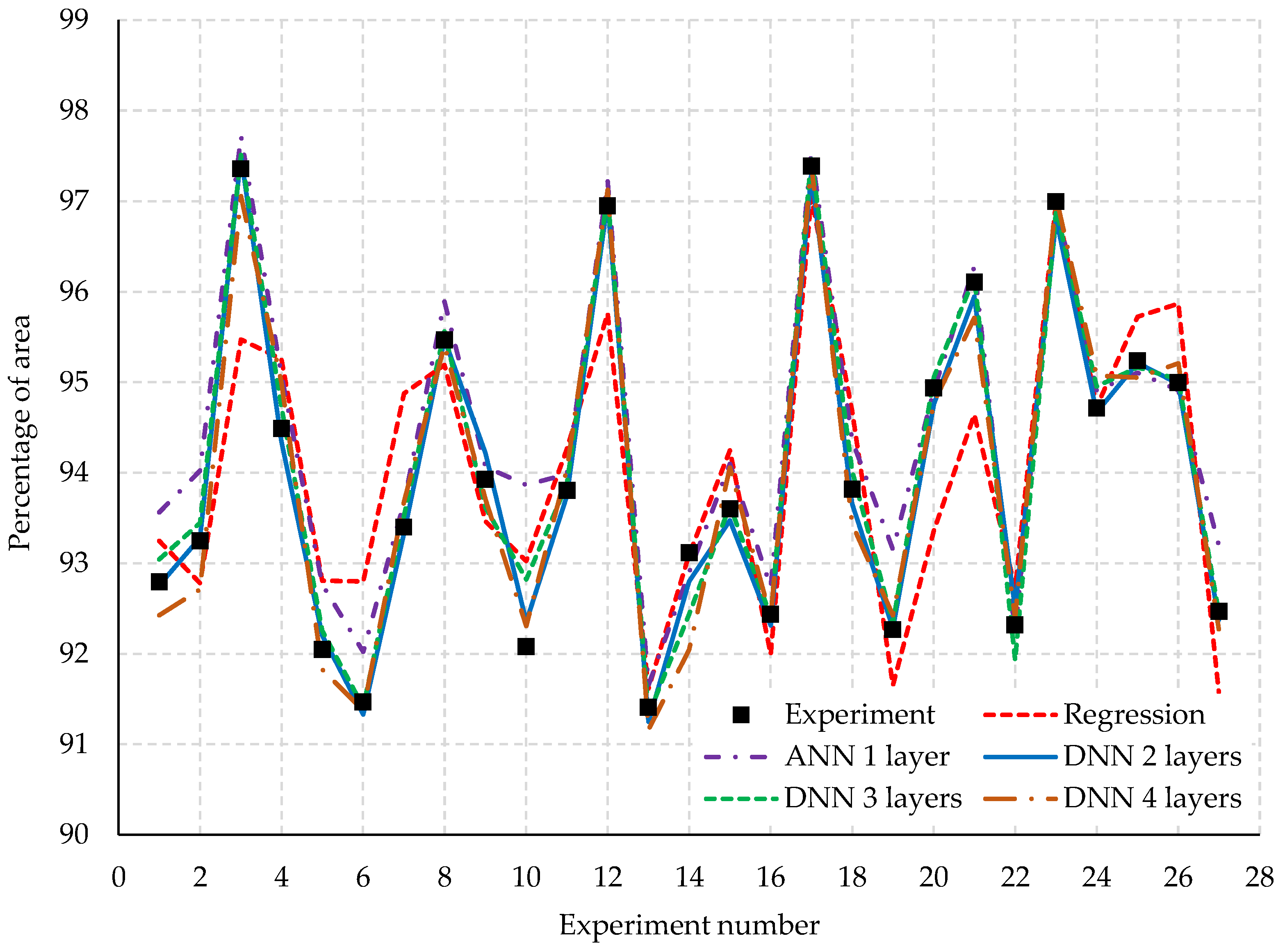
This research investigated the optimization of the process parameters to minimize springback in the Reinforcement-CTR PLR forming process. The automotive part was produced from AHSS grade JSC980Y. The four material models’ prediction performance was compared. Three process parameters: blank holder force, die clearance, and blank width were optimized. The optimization objective maximized the percentage of area within a specific displacement range between the desired shape and the predicted shape after springback occurred. In the simulation stage, the Barlat 1989 combined with the Y–U model was used in FEM simulation as the most accurate material model. The experiment was conducted with a full factorial design. Each process parameter varied with three levels. The experiment data were used for analysis with statistical regression. Additionally, the four types of ANN models were developed to compare the accuracy prediction performance with the regression model and the experimental results. Finally, the DNN with two hidden layers was selected to predict and optimize the process parameters to reach the maximum percentage of the area. The experimental results can be summarized as follows:

• The use of the Y–U hardening model is more accurate than the isotropic hardening model.
• The most accurate material model in the FEM simulation for this work is the Barlat 1989 combined with Y–U model.
• The DNN with two hidden layers is the most accurate predictive tool compared to regression and other ANN models.
• The ANN model can significantly exceed the regression models in terms of prediction accuracy.
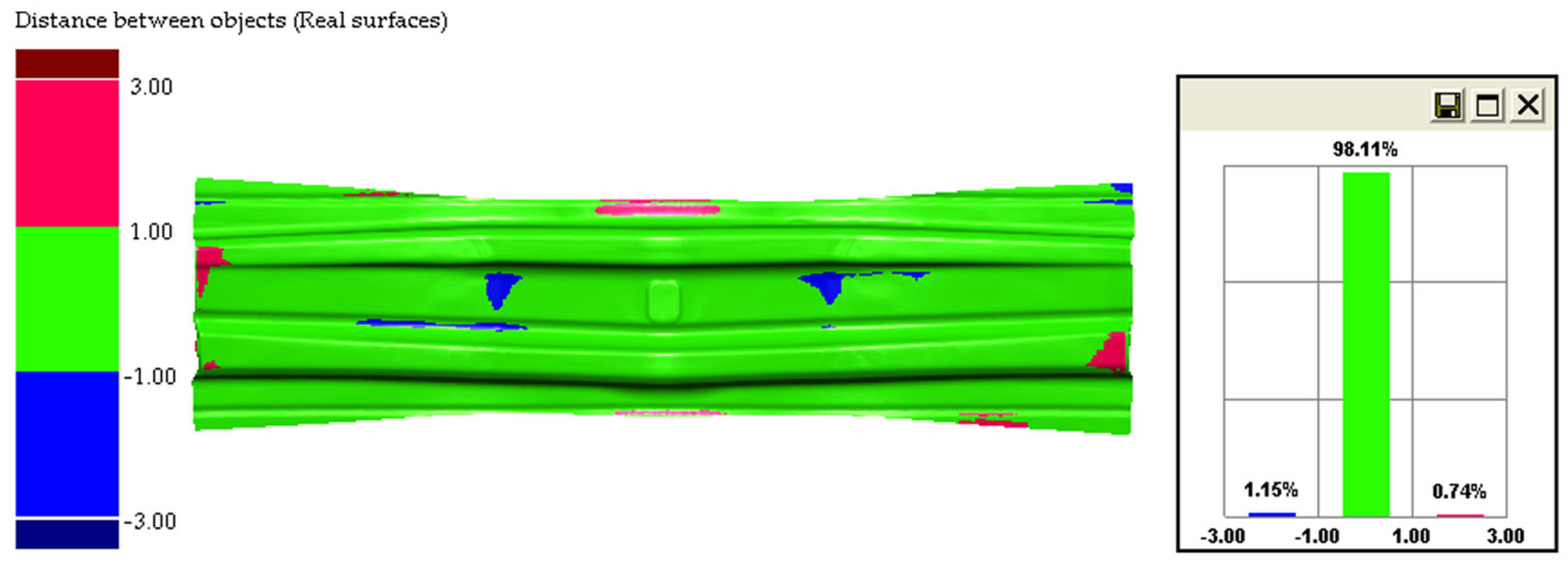
• The optimal process parameters of this work are a blank holder force of 27.62 tons, die clearance of 1 mm, and blank width of 290 mm, which achieved the percentage of area of 98.05% when optimized with an optimization algorithm and predicted by the two hidden layers DNN model at 98.11%, as obtained from the experiment.

These determined results suggest that DNN models offer a powerful and adaptable tool for optimizing complex forming processes. The method we presented is not just for this specific part or material. It combines accurate material modeling, FEM simulation, and DNN-based prediction for optimization. This creates a general approach that can be used for many different automotive parts and other AHSS types to reduce springback. As we showed, being able to accurately predict and reduce springback helps manufacturers achieve very precise shapes and, as demonstrated, can significantly improve manufacturing efficiency, reduce costly trial and error in die compensation, and enhance overall product quality. This contributes to faster development cycles and cost savings in the production of lightweight and safe vehicle structures in the automotive industry.

While the results of this study are promising, it is important to acknowledge certain limitations and highlight avenues for future research. The findings presented are specific to the AHSS grade JSC980Y and the Reinforcement-CTR PLR automotive part geometry.

For training and testing our ANN/DNN models, we split our data (80% for training, 10% for validation, and 10% for testing). This is a common way to start, especially when comparing several model designs. However, our dataset only had 27 experimental points. With such a small dataset, the way data are split can greatly affect the results. A method called K-fold cross-validation [44] is often better for small datasets. It uses all data for both training and testing in different rounds, which shows a more reliable measure of how well the model performs with new data. K-fold does take more computing time, especially if we also need to adjust many model settings (hyperparameters) for different ANN designs. For future studies that need the most thorough model checking, using K-fold would be very helpful.

Furthermore, the Yoshida–Uemori hardening model was calibrated using single-cycle tension–compression data due to equipment limitations, as mentioned in Section 2.2.2. While this provided the most accurate springback prediction among the models tested for the primarily monotonic loading conditions in critical regions of our specific forming process, incorporating multi-cycle test data for Y–U model calibration would undoubtedly enhance its predictive reliability for forming processes involving more complex cyclic loading paths.

Future research could therefore focus on (1) applying and validating this methodology with other AHSS grades and diverse automotive part complexities; (2) expanding the range and types of process parameters investigated, potentially exploring regions beyond the specific parameters established in this study; (3) incorporating more comprehensive material characterization data, including multi cycle tension–compression tests; (4) implementing K-fold cross-validation for more rigorous model evaluation and comparisons across all predictive techniques; and (5) exploring hybrid AI models or alternative machine learning techniques to potentially achieve further improvements in prediction and optimization accuracy for springback.

References

1. Lai, M.; Brun, R. Latest Developments in Sheet Metal Forming Technologies and Materials for Automotive Application: The Use of Ultra High Strength Steels at Fiat to Reach Weight Reduction at Sustainable Costs. Key Eng. Mater. 2007, 344, 1–8. [Google Scholar] [CrossRef]
2. Komgrit, L.; Hamasaki, H.; Hino, R.; Yoshida, F. Elimination of Springback of High-Strength Steel Sheet by Using Additional Bending with Counter Punch. J. Mater. Process Technol. 2016, 229, 199–206. [Google Scholar] [CrossRef]
3. Lawanwong, K.; Hamasaki, H.; Hino, R.; Yoshida, F. Double-Action Bending for Eliminating Springback in Hat-Shaped Bending of Advanced High-Strength Steel Sheet. Int. J. Adv. Manuf. Technol. 2020, 106, 1855–1867. [Google Scholar] [CrossRef]
4. Julsri, W.; Suranuntchai, S.; Uthaisangsuk, V. Finite Element Based Analysis of Two-Stage Forming for Advanced High Strength Steel Part. Procedia Manuf. 2018, 15, 668–675. [Google Scholar] [CrossRef]
5. Gan, W.; Wagoner, R.H. Die Design Method for Sheet Springback. Int. J. Mech. Sci. 2004, 46, 1097–1113. [Google Scholar] [CrossRef]
6. Lingbeek, R.; Huétink, J.; Ohnimus, S.; Petzoldt, M.; Weiher, J. The Development of a Finite Elements Based Springback Compensation Tool for Sheet Metal Products. J. Mater. Process Technol. 2005, 169, 115–125. [Google Scholar] [CrossRef]
7. Montgomery, D.C. Design and Analysis of Experiments; John Wiley & Sons: Hoboken, NJ, USA, 2017; ISBN 1119113474. [Google Scholar]
8. Özdemir, M. Optimization of Spring Back in Air V Bending Processing Using Taguchi and RSM Method. Mechanics 2020, 26, 73–81. [Google Scholar] [CrossRef]
9. Ingarao, G.; Lorenzo, R.D.; Micari, F. Analysis of Stamping Performances of Dual Phase Steels: A Multi-Objective Approach to Reduce Springback and Thinning Failure. Mater. Des. 2009, 30, 4421–4433. [Google Scholar] [CrossRef]
10. Moor, J. The Dartmouth College Artificial Intelligence Conference: The Next Fifty Years. AI Mag. 2006, 27, 87. [Google Scholar]
11. Michalski, R.S.; Carbonell, J.G.; Mitchell, T.M. Machine Learning: An Artificial Intelligence Approach; Springer Science & Business Media: Berlin/Heidelberg, Germany, 2013; ISBN 366212405X. [Google Scholar]
12. Haenlein, M.; Kaplan, A. A Brief History of Artificial Intelligence: On the Past, Present, and Future of Artificial Intelligence. Calif. Manag. Rev. 2019, 61, 5–14. [Google Scholar] [CrossRef]
13. LeCun, Y.; Bengio, Y.; Hinton, G. Deep Learning. Nature 2015, 521, 436–444. [Google Scholar] [CrossRef] [PubMed]
14. Spathopoulos, S.C.; Stavroulakis, G.E. Springback Prediction in Sheet Metal Forming, Based on Finite Element Analysis and Artificial Neural Network Approach. Appl. Mech. 2020, 1, 97–110. [Google Scholar] [CrossRef]
15. Narayanasamy, R.; Padmanabhan, P. Comparison of Regression and Artificial Neural Network Model for the Prediction of Springback during Air Bending Process of Interstitial Free Steel Sheet. J. Intell. Manuf. 2012, 23, 357–364. [Google Scholar] [CrossRef]
16. El Mrabti, I.; Touache, A.; El Hakimi, A.; Chamat, A. Springback Optimization of Deep Drawing Process Based on FEM-ANN-PSO Strategy. Struct. Multidiscip. Optim. 2021, 64, 321–333. [Google Scholar] [CrossRef]
17. Mirjalili, S.; Mirjalili, S. Genetic Algorithm. In Evolutionary Algorithms and Neural networks: Theory and Applications; Springer: Berlin/Heidelberg, Germany, 2019; pp. 43–55. [Google Scholar]
18. Kennedy, J.; Eberhart, R. Particle Swarm Optimization. In Proceedings of the ICNN’95-International Conference on Neural Networks, Perth, Australia, 27 November–1 December; IEEE: New York, NY, USA, 1995; Volume 4, pp. 1942–1948. [Google Scholar]
19. Kaelbling, L.P.; Littman, M.L.; Moore, A.W. Reinforcement Learning: A Survey. J. Artif. Intell. Res. 1996, 4, 237–285. [Google Scholar] [CrossRef]
20. Committee, E. Test Methods for Tension Testing of Metallic Materials; ASTM International: West Conshohocken, PA, USA, 2011. [Google Scholar]
21. Sanrutsadakorn, A.; Jhonthong, N.; Julsri, W. Finite Element Modeling for Analyzing the Production of High-Strength Steel Sheets for Automobile Parts. Mater. Res. Express 2024, 11, 106524. [Google Scholar] [CrossRef]
22. Yoshida, F.; Uemori, T. A Model of Large-Strain Cyclic Plasticity Describing the Bauschinger Effect and Workhardening Stagnation. Int. J. Plast. 2002, 18, 661–686. [Google Scholar] [CrossRef]
23. Julsri, W.; Suranuntchai, S.; Uthaisangsuk, V. Study of Springback Effect of AHS Steels Using a Microstructure Based Modeling. Int. J. Mech. Sci. 2018, 135, 499–516. [Google Scholar] [CrossRef]
24. Hill, R. A Theory of the Yielding and Plastic Flow of Anisotropic Metals. Proc. R. Soc. Lond. A Math. Phys. Sci. 1948, 193, 281–297. [Google Scholar]
25. Hencky, H. Zur Theorie Plastischer Deformationen Und Der Hierdurch Im Material Hervorgerufenen Nachspannungen. ZAMM-J. Appl. Math. Mech. 1924, 4, 323–334. [Google Scholar] [CrossRef]
26. Barlat, F.; Richmond, O. Prediction of Tricomponent Plane Stress Yield Surfaces and Associated Flow and Failure Behavior of Strongly Textured Fcc Polycrystalline Sheets. Mater. Sci. Eng. 1987, 95, 15–29. [Google Scholar] [CrossRef]
27. Hosford, W.F. On Yield Loci of Anisotropic Cubic Metals. In Proceedings of the Seventh North American Metal Working Conference SME, Dearborn, MI, USA, 15 May 1979; pp. 191–197. [Google Scholar]
28. Koreček, D.; Solfronk, P.; Sobotka, J. Analysis of TRIP Steel HCT690 Deformation Behaviour for Prediction of the Deformation Process and Spring-Back of the Material via Numerical Simulation. Materials 2024, 17, 535. [Google Scholar] [CrossRef] [PubMed]
29. Chaboche, J.L.; Rousselier, G. On the Plastic and Viscoplastic Constitutive Equations—Part I: Rules Developed With Internal Variable Concept. J. Press. Vessel. Technol. 1983, 105, 153–158. [Google Scholar] [CrossRef]
30. Yoshida, F.; Uemori, T.; Fujiwara, K. Elastic–Plastic Behavior of Steel Sheets under in-Plane Cyclic Tension–Compression at Large Strain. Int. J. Plast. 2002, 18, 633–659. [Google Scholar] [CrossRef]
31. Mukerjee, R.; Wu, C.F.J. A Modern Theory of Factorial Design; Springer Science & Business Media: Berlin/Heidelberg, Germany, 2007; ISBN 0387373446. [Google Scholar]
32. Draper, N.R.; Smith, H. Applied Regression Analysis; John Wiley & Sons: Hoboken, NJ, USA, 1998; Volume 326, ISBN 0471170828. [Google Scholar]
33. Ryan, T.P. Modern Regression Methods; John Wiley & Sons: Hoboken, NJ, USA, 2008; Volume 655, ISBN 0470081864. [Google Scholar]
34. Aggarwal, C.C. Neural Networks and Deep Learning; Springer: Berlin/Heidelberg, Germany, 2018; Volume 10, ISBN 3030068560. [Google Scholar]
35. Nielsen, M.A. Neural Networks and Deep Learning; Determination Press: San Francisco, CA, USA, 2015; Volume 25. [Google Scholar]
36. Abadi, M.; Agarwal, A.; Barham, P.; Brevdo, E.; Chen, Z.; Citro, C.; Corrado, G.S.; Davis, A.; Dean, J.; Devin, M. Tensorflow: Large-Scale Machine Learning on Heterogeneous Distributed Systems. arXiv 2016, arXiv:1603.04467. [Google Scholar]
37. Gulli, A.; Pal, S. Deep Learning with Keras; Packt Publishing Ltd.: Birmingham, UK, 2017; ISBN 1787129039. [Google Scholar]
38. Li, L.; Jamieson, K.; DeSalvo, G.; Rostamizadeh, A.; Talwalkar, A. Hyperband: A Novel Bandit-Based Approach to Hyperparameter Optimization. J. Mach. Learn. Res. 2018, 18, 1–52. [Google Scholar]
39. Kingma, D.P.; Ba, J. Adam: A Method for Stochastic Optimization. arXiv 2014, arXiv:1412.6980. [Google Scholar]
40. Klambauer, G.; Unterthiner, T.; Mayr, A.; Hochreiter, S. Self-Normalizing Neural Networks. In Proceedings of the Neural Information Processing Systems, Long Beach, CA, USA, 4–9 December 2017; Volume 30. [Google Scholar]
41. Willmott, C.J.; Matsuura, K. Advantages of the Mean Absolute Error (MAE) over the Root Mean Square Error (RMSE) in Assessing Average Model Performance. Clim. Res. 2005, 30, 79–82. [Google Scholar] [CrossRef]
42. Hawkins, D.M. The Problem of Overfitting. J. Chem. Inf. Comput. Sci. 2004, 44, 1–12. [Google Scholar] [CrossRef]
43. Olsson, D.M.; Nelson, L.S. The Nelder-Mead Simplex Procedure for Function Minimization. Technometrics 1975, 17, 45–51. [Google Scholar] [CrossRef]
44. Nti, I.K.; Nyarko-Boateng, O.; Aning, J. Performance of Machine Learning Algorithms with Different K Values in K-Fold Cross-Validation. Int. J. Inf. Technol. Comput. Sci. 2021, 13, 61–71. [Google Scholar]
Figure 1. Workflow diagram of this research.
Jmmp 09 00197 g001
Figure 2. The Reinforcement-CTR PLR automotive part.
Jmmp 09 00197 g002
Figure 3. True stress–strain curves of JSC980Y for each direction.
Jmmp 09 00197 g003
Figure 4. Cyclic true stress–strain curve of JSC980Y AHSS.
Jmmp 09 00197 g004
Figure 5. Setup of the forming tools within the FEM software environment.
Jmmp 09 00197 g005
Figure 6. The Reinforcement-CTR PLR automotive part prepared for 3D scanning.
Jmmp 09 00197 g006
Figure 7. Superimposition of the 3D scanned actual part (green) and the FEM simulation results (gray) after alignment using the Bestfit transformation.
Jmmp 09 00197 g007
Figure 8. Color map model of displacement between the simulated result and actual workpiece.
Jmmp 09 00197 g008
Figure 9. Color map model of displacement between before and after springback occurred.
Jmmp 09 00197 g009
Figure 10. Material models comparison results within displacement range of −1 to 1 mm.
Jmmp 09 00197 g010
Figure 11. Normal probability plot of residuals for the regression model.
Jmmp 09 00197 g011
Figure 12. Plot of residuals versus fitted values for the regression model.
Jmmp 09 00197 g012
Figure 13. Plot of residuals versus observation order for the regression model.
Jmmp 09 00197 g013
Figure 14. Training and validation loss curves: (a) 1 hidden layer, (b) 2 hidden layers, (c) 3 hidden layers, and (d) 4 hidden layers.
Jmmp 09 00197 g014
Figure 15. Comparative prediction accuracy of the regression, ANN, and DNN models.
Jmmp 09 00197 g015
Figure 16. Process parameters optimization flowchart.
Jmmp 09 00197 g016
Figure 17. FEM prediction confirmation results.
Jmmp 09 00197 g017