Abstract
Defect detection in acoustically matched media remains a significant challenge, particularly when defects, such as fiberglass and polyamide residues, exhibit properties that match those of fiber-reinforced composite laminates as the base material. Techniques, such as through-transmission ultrasound (TTU), often miss subtle residues as defects with the use of conventional amplitude-based TTU detection alone. There is a noticeable research gap in properly identifying such subtle residues in composites using TTU inspection. This study investigated the use of neural networks (NNs) to identify subtle defects in composites based on domain-specific feature extraction from TTU signals. Each signal waveform of each spatial TTU inspection is used as a discrete sample to obtain a larger dataset for each specimen. Domain-specific features were extracted separately from the time, frequency, and wavelet domains, resulting in independent feature vectors to emphasize the signal characteristics. The NN classification used 70% of the overall dataset for training and 30% for testing. Results reveal the features of the time- and frequency domains perform well, achieving macro-F1 scores of 0.96 and 0.97, respectively, while wavelet domain features perform lower with a macro-F1 score of 0.62. Wavelet-domain features perhaps need machine learning methods like recurrent NNs to correctly recognize subtle time-dependent signal variations.
1. Introduction
1.1. Nondestructive Evaluation (NDE) with Ultrasound
Ultrasonic evaluation uses piezoelectric ceramic materials to convert electrical energy into mechanical-strain waves. The high sensitivity of these materials makes them well-suited for detecting strain oscillations at ultrasonic frequencies. The evaluation was conducted by emitting a controlled ultrasonic pulse into the test article. If the same emitting transducer receives the reflected signal, the method is referred to as the echo-mode. Alternatively, when a second opposing transducer is used to receive the transmitted signal on the opposite side, this technique is called through-transmission ultrasound (TTU). The ultrasonic signal transmitted through the article consists of pulse waves, that is, short bursts of longitudinal compression waves centered around a certain frequency. In the echo-mode setup illustrated in Figure 1a, the pulse reflects off boundaries, such as the front surface, internal defects, and back surface, returning as time-separated echoes. In the defect-free regions, waves pass through the material without reflection. When a defect is present, part of the wave is reflected, and the strength of this reflection is related to the acoustic impedance mismatch between the defect and the surrounding material of the test article. Echo-mode evaluation does not require manual thresholding across varying counts, as time-corrected gain (TCG) can be applied to automatically compensate for attenuation and geometric effects at each depth.
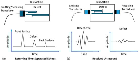
Figure 1.
Schematic comparison of (a) echo-mode and (b) through-transmission (TTU) ultrasonic evaluation methods. In the echo-mode, a pulse is reflected off the internal interfaces and surfaces based on acoustic impedance differences, returning time-separated echoes. In the TTU mode, a pulse travels through the material, with defects causing attenuation or absence of the signal on the opposite side, as received echoes, owing to the impedance mismatch.
By contrast, in the TTU system shown in Figure 1b, a transducer emits a pulse through the test article to the receiving transducer on the opposite side. In defect-free regions, waves pass through with minimal attenuation. When a defect is present, the wave may be partially or completely blocked because of the impedance difference, leading to a weak or absent signal on the received side. TTU systems must rely on conventional manual thresholding of transmitted amplitude, which becomes increasingly difficult when inspecting materials with varying counts and subtle impedance differences.
Figure 2 illustrates the acoustic impedance mismatch between the typical evaluation media and its significant effect on wave propagation. When an ultrasonic wave travels from water into an FRC laminate, approximately 26% of the wave is reflected by impedance mismatch. However, when the wave transitions from the FRC laminate to air, 99.93% of the wave energy is reflected, indicating a large acoustic impedance difference.
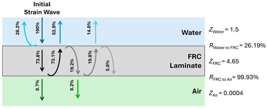
Figure 2.
Reflection and transmission coefficients for ultrasonic waves interacting with water, FRC laminate, and air. The reflection coefficient at the water–FRC laminate interface was 26.19%, whereas complete reflection (99.93%) occurred at the FRC–air interface owing to the significant impedance mismatch [1].
In contrast, residual materials, such as fiberglass and polyamide release fabrics, transmit approximately 97.94% and 92.78% of the signal, respectively, when paired with the FRC laminate as the base material. This results in a difference of only 2% and 7% in the received signal, leading to attenuation differences that are too subtle for conventional amplitude-based TTU systems to reliably detect, given the small acoustic impedance difference [1].
This subtlety creates a significant challenge for TTU evaluation in production environments, where the echo-mode may be impractical owing to a variety of constraints emphasized in the following literature review. Consequently, identifying such defects, particularly when embedded within acoustically matched FRC laminates, remains one of the most difficult challenges in nondestructive evaluation (NDE). In such cases, conventional TTU, which lacks echo-mode, advanced classification thresholds that would otherwise require manual thresholding, may fail to detect subtle anomalies [1].
The preceding TTU limitations highlight the need for automated machine learning approaches, such as neural networks, to aid in improving defect detection reliability and consistency in TTU inspections of acoustically matched media across varying counts.
1.2. Neural Network Classification
The accurate classification of ultrasound waveforms is critical in the field of NDE ultrasound testing, particularly for identifying internal defects in FRC laminates [2]. An accurate interpretation of ultrasonic wave behavior requires a thorough understanding of advanced signal processing techniques to analyze complex waveforms, extract relevant features, and apply appropriate machine learning models. Feature extraction methods reduce data complexity to relevant information, highlighting patterns to improve classification performance in machine learning models, such as neural networks. This process helps to detect defects, characterize materials, and identify underlying signal behaviors that might otherwise remain hidden.
Distinctive features can be extracted for further analysis. In this study, engineering features were extracted independently from the time-, frequency-, and wavelet-domains. The time-domain features reflect how the signal changes over time, whereas the frequency-domain features, typically obtained through Fourier analysis, reveal the periodic components and energy content. In addition, wavelet-domain features combine both time- and frequency-domain information, which is valuable for TTU signal analysis where subtle localized anomalies may be missed when analyzed in either domain alone [3].
Neural networks (NNs) were selected as the classification model owing to their ability to learn and generalize complex nonlinear relationships within rich feature datasets. They have been applied in ultrasonic evaluation tasks such as evaluating the health of ceramic insulators using ultrasonic signals [4].
1.3. Advancing TTU in Acoustically Matched Media
The focus of this study addresses the specific challenge of detecting acoustically matched foreign materials in FRC laminates. In contrast, defect types, such as porosity or delamination, which produce strong acoustic impedance mismatches, can typically be detected using standard TTU techniques without the need for machine learning classification [2].
To advance TTU-based evaluations for detection of acoustically matched media, this study evaluated the use of NNs to classify such defects in FRC laminates. Instead of combining all features into a single vector, the feature sets were separated by domain (time, frequency, and wavelet) to independently assess their discriminative power. Each pixel-level waveform provided an individual sample of 1764 pixels as the dataset, split randomly into 70% training and 30% testing sets to evaluate the model performance without data leakage.
The results showed that the time- and frequency-domain features enabled high defect classification accuracy, achieving macro-F1 scores of 0.96 and 0.97 respectively. The wavelet-domain features provided lower performance, with a macro-F1 score of 0.62, suggesting that mid-frequency localized information alone may be insufficient for this application. These findings demonstrate the importance of domain-specific feature engineering and confirm that time- and frequency-domain representations are particularly effective for the TTU inspection of acoustically matched defects in composites. Artificial neural networks offer a scalable and reliable solution where traditional methods lack sensitivity for industrial based NDE.
Future work will explore feature fusion strategies combining time-, frequency-, and wavelet-domain features into integrated representations as well as the use of convolutional neural networks (CNNs) and spiking neural networks (SNNs) to enhance automated defect detection in more complex materials and evaluation scenarios.
2. Motivation
2.1. Background: Ultrasound Evaluation and Waveform Classification
Ultrasound evaluation and waveform classification play key roles in NDE because of their ability to accurately detect internal defects across a wide range of materials [5]. Echo-mode techniques are well established for defect localization and depth detection [6]. However, these techniques present a challenge when inspecting thin materials, excessive ramps, tapered structures, and areas with limited front surface access [7,8].
TTU is a viable alternative that provides consistent signal transmission when reflections are diminished or unreliable [9]. However, its effectiveness depends heavily on the acoustic contrast between the materials. For example, in FRC laminates with acoustically matched defects, the lack of a significant acoustic impedance mismatch reduces the contrast in the transmitted waveforms, with only small differences (approximately 2% and 7%, respectively) in signal transmission. This subtle attenuation makes it challenging for conventional TTU systems to reliably detect anomalies, particularly when the impedance differences are too small to produce a noticeable contrast in the received signals. Echo-mode time-of-flight techniques are well-suited to minor impedance differences [5,6]. Therefore, the use of TTU must be explored further to improve defect recognition in acoustically matched media in FRC laminates.
2.2. Feature Extraction: Time, Frequency, and Wavelet Domains
Reliable classification of the received ultrasonic signals depends on accurate feature extraction. Time-domain features such as the peak amplitude, root mean square (RMS), signal energy, and signal duration capture variations in amplitude over time and are valued for their simplicity and speed [10]. Signal processing methods with Fourier analysis can reveal subtle spectral deviations associated with internal structural changes and can serve as model-based approaches for ultrasonic echo analysis [11,12]. More recently, specific wavelet shapes and parameters have been studied and developed for signal analysis, and wavelet transforms have gained traction owing to their ability to capture transient and nonstationary features that are often critical in NDE applications [13,14,15]. Despite advancements in signal processing, it is uncommon to separately evaluate and compare the time-, frequency-, and wavelet-domain features in TTU data, particularly for detecting subtle defects in acoustically matched fiber-reinforced composite (FRC) laminates.
2.3. Machine Learning: Neural Network Classification
Recent advances in machine learning have provided more sophisticated approaches that move beyond traditional thresholding and signal processing methods. Traditional NNs, a class of feedforward neural networks or multi-layer perceptrons, have been widely adopted because of their ability to model complex nonlinear relationships and classify subtle patterns within rich feature datasets. NNs have been widely adopted because of their flexibility in modeling ultrasonic signals, classifying various defect types, using backpropagation for accuracy, and effectively modeling complex nonlinear relationships [16,17,18].
For example, Chen et al. [19] used TTU-acquired ultrasonic data and neural networks to classify the porosity of CFRP composites. Similarly, Huang et al. [20] employed deep learning models to analyze TTU data from air-coupled transducers to improve defect detection. Although these studies have confirmed that neural networks can be applied to TTU data, such work remains an exception rather than a rule. In this study, NNs were developed to classify ultrasonic waveform signals based on domain-specific feature sets extracted independently from time, frequency, and wavelet domains. Each pixel-level waveform is treated as an individual sample to enable a more detailed and rich classification framework. Therefore, this research addresses a critical gap by applying domain-specific pixel-level feature extraction and NN classification to TTU inspection of acoustically matched media, thereby improving sensitivity to subtle signal variations.
2.4. Bridging Research Gaps
Although machine learning models, such as NNs, have been applied in ultrasonic research, their use remains relatively limited for TTU. Furthermore, domain-specific feature extraction for TTU inspection has not been systematically investigated, particularly in acoustically matched media where baseline and defect signals are difficult to distinguish using conventional amplitude-based TTU methods. Additionally, there has been little work at the pixel level, where more granular signal variations can be captured and analyzed. There is a need for systematic evaluation of how features from different domains independently contribute to defect classification performance. Addressing these gaps is essential for improving acoustically matched defect recognition using TTU.
This study addresses these challenges by evaluating NN classifiers trained on domain-specific feature sets extracted separately from time, frequency, and wavelet domains. Rather than combining all the features into a single vector, independent feature extraction and classification were performed to better understand the discriminative power of each domain. Each pixel-level waveform was treated as an individual sample, and the NN classification performance was assessed using domain-specific feature sets. The results highlight that time and frequency-domain features provide high classification performance for TTU inspection of acoustically matched media in FRC laminates, while wavelet-domain features perform lower and less discriminative in isolation. This study offers a novel domain-specific machine learning framework that noticeably improves the sensitivity of TTU inspection to detect subtle defects in acoustically matched media, providing an alternative to conventional amplitude-based TTU methods.
3. Materials and Methods
3.1. Dataset Description
Ultrasonic waveform data were collected using a TTU setup with a 5 MHz transducer operating at a normal incidence angle (0°) with a 4.00-inch water column standoff. The representative reference standard, designed to reflect aerospace thin-wall structural properties, was an FRC laminate containing known baseline regions, classified as having no defects, and regions with embedded fiberglass and polyamide inserts serving as artificial acoustically matched defects. The TTU setup parameters are summarized in Table 1, and the representative reference standards are illustrated in Figure 3. The dataset was balanced, ensuring an equal distribution of the baseline and defect classes to facilitate reliable performance assessment.

Table 1.
TTU Method Setup for Pixel-Level TTU of FRC Laminates.
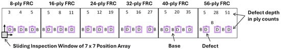
Figure 3.
Representative standard drawing illustrating the 18 baselines (B) and defects (D), with 36 total waveforms of 49 pixels, equaling 1764 points [1]. Defects are highlighted in purple.
The reference standard was scanned using a spatial grid of 0.08 × 0.08 inches with a sampling period of 0.02 microseconds. Waveform data were collected and stored as a function of the scan (m), index (n) position, and time (t), with an acquisition gate used to capture the peak amplitude values within each A-scan signal. Each extracted sample was arranged in a 7 × 7 matrix array, yielding 49 pixel-level waveform signals per region.
The final dataset consisted of 1764 pixel-level waveforms distributed equally between the baseline and defect classes. Each baseline and defect area were extracted across six different ply counts (8, 16, 24, 32, 40, and 56 plies) to ensure a balanced distribution across geometry configurations. Pixel-level analysis allows high-resolution defect detection without averaging across large regions.
Voltage-to-color mapping was applied to enhance the visual contrast between the baseline and defect signals. The peak signal amplitude (Vhigh) was set to white, amplitudes between the threshold (Vthreshold) and the lowest signal amplitude (Vlow) were set to red, and signal amplitudes above the threshold (Vthreshold) were mapped to a color pallet using 256 shades of grey gradient.. This mapping maximized the contrast within the acquired C-scan images, helping to visually differentiate between baseline regions (typically exhibiting higher amplitudes) and defect regions (typically exhibiting lower amplitudes). Figure 4 illustrates the pixel-level extraction process based on this mapping.
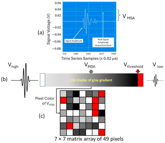
Figure 4.
This figure illustrates the generation of a pixel-level dataset using the TTU scanning process. (a) shows the TTU signal amplitude (VMSA) at a position in volts and peak acquisition gate, (b) corresponding voltage-to-color mapping illustrating that the peak signal amplitude (Vhigh) was set to white, amplitudes between the threshold (Vthreshold) and the lowest signal amplitude (Vlow) were set to red, and signal amplitudes above the threshold (Vthreshold) were mapped to a color pallet using 256 shades of grey gradient, and (c) shows the resulting two-dimensional position array, where each 7 × 7 matrix array of 49 pixels was extracted as an individual sample from either the baseline or defect regions, resulting in a total of 1764 pixel-level waveforms across the dataset [1].
3.2. Feature Extraction
Accurate classification of ultrasonic signals depends on the extraction of discriminative features from each waveform, which captures essential signal characteristics. In this study, feature extraction was performed independently at the pixel level to preserve localized variation across the scanned regions. Each pixel waveform is processed to extract domain-specific features separately from the time-, frequency-, and wavelet-domains.
Sixteen features were extracted across the three domains to provide a comprehensive representation of the ultrasonic waveform: 6 from the time-domain, 5 from the frequency domain, and 5 from the wavelet domain. Separate NN models were trained for each domain independently, with the number of input neurons corresponding to the number of features from that domain. The selected features describe key properties, such as signal intensity, energy dispersion, asymmetry, spread, and oscillatory behavior, forming the foundation for the classification models developed in this study. The specific features extracted from each domain along with their physical units are summarized in Table 2.
Table 2.
Summary of extracted feature descriptions and units categorized by domain.
3.2.1. Time Domain
The time domain describes how ultrasonic signals vary as a function of time. The time-domain features capture the amplitude-based characteristics and statistical properties of the waveform, which can reflect the presence of internal discrepancies that can be further characterized as defects. Common domain metrics include peak amplitude, mean amplitude, root mean square (RMS) amplitude, and statistical descriptors such as variance, skewness, and kurtosis.
Figure 5 presents a representative ultrasonic waveform signal (black line) annotated with key time-domain features, including the mean signal level (dotted green line), peak amplitude (maximum signal as red dot), trough amplitude (minimum signal as blue dot), and ± RMS amplitude boundaries (dotted blue horizontal lines). These features were directly extracted from each pixel-level waveform and served as inputs for subsequent classification.
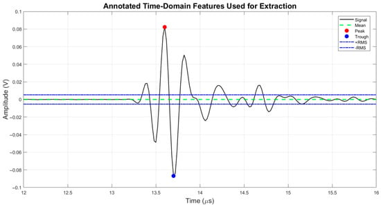
Figure 5.
The annotated time-domain features were extracted from a representative ultrasonic waveform, highlighting the mean amplitude, peak-to-peak values (peak and trough), and RMS amplitude boundaries. The variance, skewness, and kurtosis were computed based on the overall signal shape and dispersion.
In this study, time-domain features were extracted directly from the raw ultrasound waveforms to quantify the amplitude characteristics and temporal signal patterns. The peak amplitude was derived from the maximum absolute value, capturing the maximum instantaneous amplitude , as defined by (1), where is the discrete time-domain signal.
The , shown in (2), estimates the waveform energy over time, where represents the amplitude at time , and is the number of samples, where ranges from 1 to N [21].
Statistical descriptors such as the mean and variance in (3) and (4), respectively, were also computed to capture the average signal intensity and spread, providing basic statistical measures of central tendency and dispersion [21].
In addition, skewness and kurtosis were used to describe the shape of the amplitude distribution to capture the asymmetry and peak amplitude, respectively, and to further characterize the signal shape for defect detection. These extracted time-domain features were used as inputs for subsequent machine learning classification models.
3.2.2. Frequency Domain
Frequency domain analysis involves transforming ultrasonic signals from the into their constituent frequency components, revealing frequency-specific characteristics that are often not visible in raw waveforms. In this study, a Fast Fourier Transform (FFT) was applied to each pixel-level waveform to enable spectral analysis and extraction of key frequency domain features.
The commonly extracted spectral features include the spectral centroid, spectral spread (standard deviation), spectral skewness, spectral kurtosis, dominant frequency, and spectral roll-off (85% cumulative energy). These features quantify the distribution, dispersion, and shape of energy across different frequency components, providing critical information for distinguishing between the baseline and defect conditions. These features are critical for detecting subtle differences between baseline and defect conditions, which are often more pronounced in the frequency domain than in the time-domain. In this study, a Fast Fourier Transform (FFT) was applied to each ultrasound waveform to enable further spectral analysis, focusing on frequency-specific information such as the spectral centroid and spectral spread.
To visualize these frequency domain features, Figure 6 presents the magnitude spectrum of a representative ultrasonic waveform annotated with the dominant frequency (peak magnitude) and spectral centroid (energy-weighted average frequency). The spectral centroid reflects where most of the spectral energy is concentrated, whereas the spectral spread characterizes how widely the frequency components are dispersed around the centroid. The dominant frequency captured the strongest oscillatory component, and the spectral roll-off indicated a frequency below which 85% of the total spectral energy was contained. A frequency range of 0–10 MHz was used for all analyses, consistent with the 5 MHz transducer bandwidth and acquisition settings.
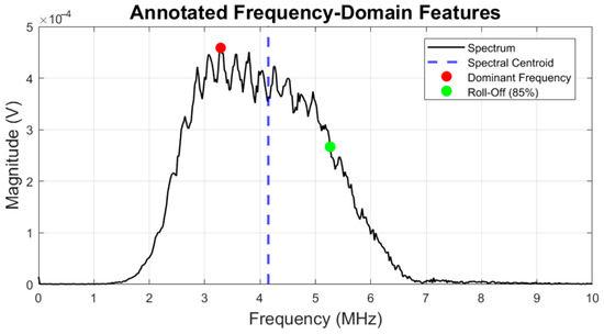
Figure 6.
Annotated frequency-domain features were extracted from a representative ultrasonic waveform, highlighting the spectral centroid, dominant frequency, and spectral roll-off (85% cumulative energy). The spectral spread, skewness, and kurtosis were computed based on the overall spectral distribution.
The frequency-domain components were computed using conventional signal processing definitions. Key spectral components were extracted using the Discrete Fourier Transform (DFT) in (5), the magnitude spectrum in (6), and centroid in (7), as defined in [22].
where represents the complex frequency coefficients at the frequency bin, is the time domain signal, is the imaginary unit, and is the number of samples.
These extracted frequency-domain features were used as inputs for subsequent machine-learning classification models.
3.2.3. Wavelet Domain
A wavelet transform is a math function that allows analyzing signals with frequency contents that evolve over time. Wavelet analysis offers a significant advantage over the traditional time- and frequency-domain methods. Unlike the sine and cosine functions used in Fourier transforms, wavelets are compact zero-mean functions that offer precise localization in both time and frequency domains. This property makes wavelets particularly suited for analyzing ultrasonic signals that exhibit transient or nonstationary characteristics, owing to their internal defects. Figure 7 illustrates the wavelet transform process, where a short-duration wavelet is convolved with the input signal over time to produce localized coefficients that reflect dynamic signal changes to produce localized coefficients reflecting time-frequency signal dynamics.
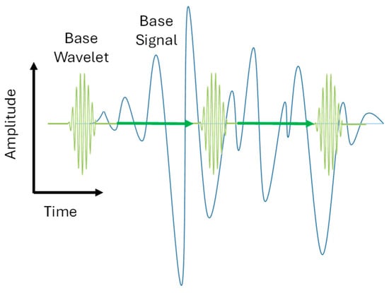
Figure 7.
Schematic representation of the wavelet transform process. A compact base wavelet with the green color is convolved with an ultrasonic base signal with the blue color to produce localized coefficients reflecting the time-frequency signal dynamics. The convolution operation is indicated by the green arrows.
In this study, wavelet domain features were extracted using a four-level Discrete Wavelet Transform (DWT) applied to each pixel-level ultrasonic waveform using the energy distribution shown in (8) and derived using a Daubechies-4 (db4) basis, as described in [14]. The sum of the squared detail coefficients, where are the detail coefficients at level . This provides a localized measure of signal activity across frequency bands.
In (8), is the energy level at and are the detail coefficients at level j, representing the decomposition at that level.
The db4 basis was selected because it is suitable for capturing the sharp transitions and oscillatory patterns that are common in ultrasonic waveforms. Figure 8 presents the distribution of the combined D3 + D4 detail coefficients from a representative waveform with the mean value and total energy annotated. Five statistical features were extracted from the combined coefficients, which are the mean, variance, skewness, kurtosis, and energy.
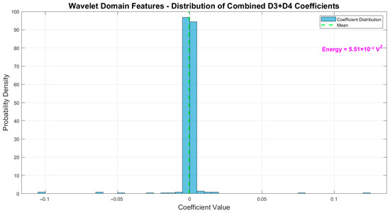
Figure 8.
DWT wavelet decomposition histogram of the combined D3 + D4 coefficients of the db4 wavelet coefficient distribution. The mean is indicated by the dashed green line, and the total energy of the detailed coefficients is annotated, highlighting the concentration of the signal energy in the mid-frequency bands.
This approach leverages time-frequency component localization using wavelet transforms utilizing feature extraction to obtain the most informative spectral region for improved defect detection. These extracted wavelet domain features were used as inputs for subsequent machine-learning classification models.
3.3. Neural Network (NN) Models
Neural networks have emerged as powerful tools for ultrasound waveform classification primarily because of their ability to automatically learn complex data patterns [23,24]. This study used a neural network classifier for comparative analysis.
NNs are first-generation feedforward neural networks comprising the input, hidden, and output layers. They used backpropagation and gradient descent to minimize classification errors. NNs have demonstrated impressive performance in ultrasonic evaluations, particularly when trained on diverse feature sets, and are considered a benchmark for signal-based classification tasks [25].
Each NN model used in this study consists of an input layer with 6-or-5-neurons corresponding to the extracted feature vector, followed by a fully connected single hidden layer with 32 neurons. The input layer of the time-domain NN model consists of 6 neurons. The input layer of the frequency or wavelet domain NN model consists of 5 neurons. A Rectified Linear Unit (ReLU) activation function was applied to the hidden layer to introduce nonlinearity. The output layer consists of a single neuron with a sigmoid activation function to perform binary classification between the baseline and defect classes.
The training algorithm used was Levenberg–Marquardt backpropagation, with a maximum of 100 training epochs and early stopping enabled after six consecutive validation failures. This algorithm uses full-batch optimization and does not require a manually specified learning rate or batch size. The architecture of NN models is summarized in Table 3 and illustrated in Figure 9.
Table 3.
NN architectures for defect classification.
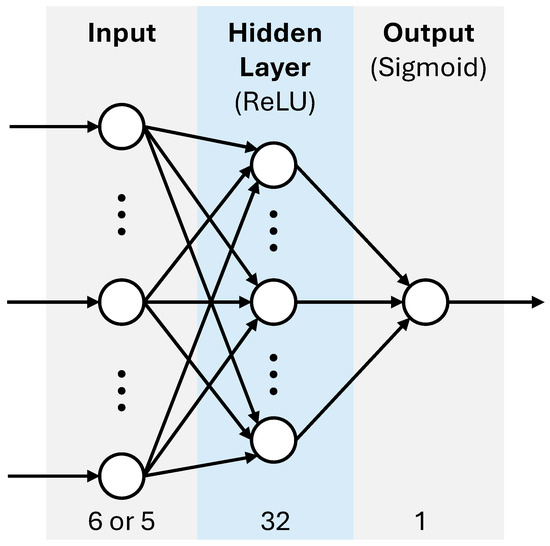
Figure 9.
This NN architecture is used for the binary classification of ultrasonic signal waveform features. The model included a 6-or-5-neuron input layer corresponding to the domain-specific input features, a fully connected hidden layer with 32 neurons using ReLU activation, and a final output layer with sigmoid activation for binary classification. The input layer of the time-domain NN has 6 neurons, but the input layer of the frequency- or wavelet domain NN has 5 neurons. The arrows are feedforward signal transmission. A multitude of neurons is represented by an ellipsis in each NN layer.
Each NN model maps the domain-specific feature vector directly onto a binary output prediction. The input features were passed through the hidden layer with the Rectified Linear Unit (ReLU) activation, as defined in (9), where x is an argument.
This activation enables the network to learn the complex nonlinear relationships between features. The output layer uses a sigmoid activation function to generate a probability output defined by (10), where x is an argument.
A binary decision was made to apply a threshold of 0.5, where probabilities greater than 0.5 were classified as defects (Class 2), and those less than or equal to 0.5, were classified as baseline (Class 1). Although class labels were mapped to 1 (baseline) and 2 (defect) for processing consistency, the binary thresholding logic remained consistent with the conventional 0/1 classification approaches.
This lightweight architecture supports efficient training and strong generalization, making it well-suited for feature-based ultrasonic defect classification. When combined with appropriate regularization techniques, it provides robust performance across pixel-level datasets. As shown in Figure 9, each NN model consists of a 6-or-5-dimensional input layer, a single hidden layer with 32 neurons using ReLU activation, and a final output neuron with sigmoid activation to produce binary results.
3.4. Experimental Design
The feature data were initially standardized using z-score normalization, which adjusts each feature such that it has a mean of zero and standard deviation of one. This approach was preferred over simple min-max scaling because it is better at handling outliers and helps neural networks learn more efficiently.
The dataset was split into 70% for training and 30% for testing, while maintaining the original balance between the baseline and defect waveform samples. During training, the training set was internally divided, with 80% used for weight updates and 20% used for internal validation to monitor model performance and prevent overfitting. Table 4 summarizes the key experimental parameters and training configurations used for NNs.
Table 4.
Summary of key experimental parameters and training configurations used for NNs.
The following metrics were used to assess the model performance:
- Accuracy: Proportion of correctly classified instances across all samples.
- Precision: Proportion of predicted defects that were true, reflecting the model’s ability to avoid false positives.
- Recall (Sensitivity): The proportion of actual defects correctly identified, which measures how effectively the model detects the true defects.
- F1-score: The harmonic mean of precision and recall is useful for balanced performance evaluation.
- Confusion Matrix: A visual representation of classification outcomes, helping to identify misclassifications and class-specific accuracy.
To ensure a balanced evaluation across the baseline and defect classes, macro averaged metrics were reported, where each class contributed equally to the overall metric calculations. This approach ensures that the classification performance is not biased toward one class, even when subtle signal differences exist between the baseline and defect conditions. Together, the feature extraction methods and classification architectures described in this section form the foundation for evaluating defect detection performance. as detailed in Section 4.
4. Results
4.1. Domain-Specific Exploratory Analysis
Acoustic detection methods, which use conventional amplitude thresholding in TTU, are known to be inadequate for reliably detecting subtle defects in acoustically matched materials, particularly when signal variability from ply count or material heterogeneity exceeds the minimal impedance contrast [6,9]. Summary statistics, including mean, variance, and skewness, were calculated for each feature within the time-, frequency-, and wavelet domains to provide a comprehensive view of the signal characteristics, highlighting the differences between the baseline and defect conditions. The exact p-values for these comparisons were calculated using paired two-sample t-tests and are summarized in Table 5. Each feature reveals important characteristics of signal behavior as the ply count changes.
Table 5.
Domain specific p-values based on t-test.
4.1.1. Time Domain Exploratory Results
Figure 10 shows the zoomed and rectified mean waveforms, comparing the baseline and defect conditions across the six ply counts. Variations in shape across the amplitude and waveform samples are typical conventional amplitude-based time-domain features used for detecting internal defects.
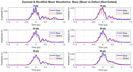
Figure 10.
Mosaic of the mean waveforms in the time-domain comparing baseline (solid blue) and defect (dashed red) across six different ply counts.
The time-domain features (a) mean, (b) variance, and (c) skewness) were calculated for both the baseline and defect across the different ply counts shown in Figure 11, highlighting the differences between the baseline and defect conditions. Each feature reveals important characteristics of signal behavior as the ply count changes.
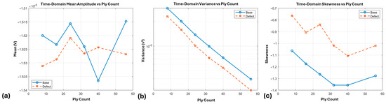
Figure 11.
Time-domain features: (a) mean amplitude vs. ply count, (b) variance vs. ply count, and (c) skewness vs. ply count for baseline and defect conditions.
The time-domain statistics, including mean, variance, and skewness, revealed p-values greater than 0.05, indicating no significant statistical distinction between the baseline and defect conditions. The mean amplitude changed slightly across ply counts, but the variations were subtle and not large enough to clearly separate defects from baseline conditions, with subtle variations observed. The variance decreased with increasing ply count, indicating more stable signals in thicker materials. The skewness values become less negative under defect conditions, indicating that defects lead to more symmetrical signal distributions in thicker materials. These findings underscore the need for neural networks to capture subtle, nonlinear patterns in which basic features such as these cannot be differentiated.
4.1.2. Frequency Domain Exploratory Results
Figure 12 compares the baseline and defect spectra across the six ply counts, depicting the spectral shifts. The differences in the spectral shifts, including the magnitude and shape, highlight the value of the frequency-domain feature for capturing defect-induced changes.
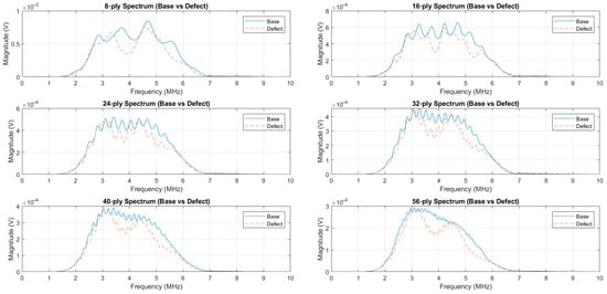
Figure 12.
Mosaic frequency spectrum comparing baseline (solid blue) and defect (dashed red) across six ply counts.
The frequency-domain spectral features (a) mean, (b) variance, and (c) skewness) were calculated for both the baseline and defect across the different ply counts shown in Figure 13, highlighting the differences between the baseline and defect conditions from a spectral analysis. Each spectral feature reveals important characteristics of the signal behavior as the ply count changes.
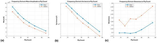
Figure 13.
Frequency-domain features: (a) mean amplitude versus ply count, (b) variance versus ply count, and (c) skewness versus ply count for baseline and defect conditions.
The p-values for the frequency-domain statistics (mean, variance, skewness) are greater than 0.05 across all ply counts, indicating no significant statistical distinction between the baseline and defect conditions. This suggests that the frequency-domain alone cannot clearly differentiate between the two conditions. The mean values remained consistent with the slight variations observed. The variance decreased with increasing ply count, indicating that thicker materials resulted in more stable frequency components. Skewness values remained positive for both conditions, becoming slightly higher as ply count increased, suggesting that defects lead to a more balanced frequency distribution in thicker materials. These findings underscore the need for neural networks to capture subtle, nonlinear patterns in which basic features such as these cannot be differentiated.
4.1.3. Wavelet Domain Exploratory Results
Figure 14 shows the wavelet decompositions across the six ply counts using db4 to illustrate how the wavelet-domain features differentiated between the baseline and defect conditions. Noticeable shifts in the energy concentration, spectral magnitude, and distribution validate the discriminative power of the mid-frequency wavelet bands, and wavelet-based analysis captures subtle anomalies that may otherwise be missed.
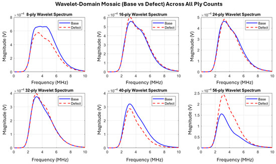
Figure 14.
Mosaic wavelet-domain comparing baseline (solid blue) and defect (dashed red) across six ply counts using db4 decomposition.
The wavelet-domain spectral features (a) mean, (b) variance, and (c) skewness were calculated for both the baseline and defect across different ply counts, as shown in Figure 15, highlighting the differences between the baseline and defect conditions. Each feature reveals important characteristics of signal behavior as the ply count changes.
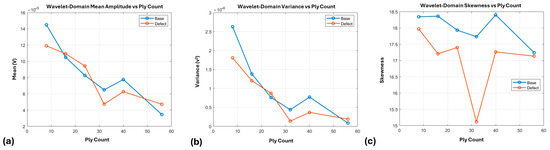
Figure 15.
Wavelet-domain features: (a) mean amplitude versus ply count, (b) variance versus ply count, and (c) skewness versus ply count for the baseline and defect conditions.
The wavelet-domain statistical analysis revealed significant differences between the baseline and defect conditions for all ply counts except 16-ply, where the p-value was 0.2317. For the other ply counts, the p-values were less than 0.05, indicating a statistically significant difference. Generally, the mean and variance values were lower for defect conditions compared to the baseline; however, this trend was not perfectly consistent across all counts. Variations were observed, with specific counts showing comparable or even slightly higher values for defect signals, reflecting the complexities inherent in the ultrasonic signal behavior across different material configurations.
These results highlight the value of wavelet-domain features in capturing localized, mid-frequency signal variations that traditional time- and frequency-domain methods might overlook. Although the time- and frequency-domain features exhibited subtle changes, they showed limited separability between the baseline and defect conditions with no statistically significant differences across ply counts.
Overall, the exploratory statistical analysis emphasized that simple feature measures alone are insufficient for reliable defect detection in acoustically matched media. These results provide motivation to take advantage of machine learning models to capture the complex nonlinear relationships needed for improved classification performance.
4.2. Neural Netowrk Classification Results
Each pixel-level waveform provided an individual sample of 1764 TTU inspection pixels as the overall dataset that was split randomly into 70% training and 30% testing sets to evaluate the NN classification without data leakage, ensuring that there was no overlap between the training and testing sets for evaluating the generalization capabilities of NNs.
4.2.1. Overview of Neural Network Training
To evaluate the effectiveness of domain-specific feature extraction, three separate NN classifiers were trained using features extracted independently from the time, frequency, and wavelet domains. Each pixel-level waveform of 1764 pixels served as an individual sample, allowing for detailed defect recognition without spatial averaging. Model performance was assessed using macro-averaged metrics, including F1-score, accuracy, precision, and recall. Macro-averaging ensured equal weighting of the baseline and defect classes regardless of the sample size.
To ensure generalization and prevent overfitting, each NN model was trained using the training set, from which a 20% validation set was further extracted to tune NN hyper-parameters like a learning rate or momentum during NN training with early stopping based on validation loss monitoring. Although a maximum of 50 training epochs was permitted, training automatically terminated once the validation loss plateaued. As a result, the models converged rapidly: the time-domain NN completed training in 4 epochs, the frequency-domain NN in 5 epochs, and the wavelet-domain NN in 3 epochs. This behavior reflects efficient learning and generalization without undertraining while utilizing the actual number of epochs completed. This early stopping protocol aligns with best practices in neural network training and provides a realistic assessment of convergence and stability than arbitrarily fixed training lengths.
The training and validation loss curves (Mean Square Error) decreased quickly across all domain-specific NN models, showing minimal divergence between training and validation sets and indicating strong generalization. Final validation loss values remained low: approximately 0.06 (time), 0.01 (frequency), and 0.14 (wavelet), respectively, confirming that each model successfully captured the relevant signal patterns without overfitting. These results demonstrate that NNs effectively learned meaningful feature relationships between baseline and defect signals during training, prior to evaluation of the independent 30% testing set. Figure 16 presents the training and validation performance curves for all three domains.
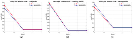
Figure 16.
Training and validation loss curves for each domain-specific NN classifier. Subplots (a), (b), and (c) correspond to the time, frequency, and wavelet domains, respectively. The NN models converged rapidly with minimal divergence between training and validation performance, indicating strong generalization and effective learning.
Figure 17 presents the confusion matrices for the pixel-level NN classifiers performed on the training set, which is 70% of the overall dataset, using the (a) time-domain, (b) frequency-domain, and (c) wavelet-domain features. Table 6 summarizes the pixel-level NN classification performance across time, frequency, and wavelet domains. The Macro-F1 score, accuracy, and confusion matrix elements (true positives, true negatives, false positives, and false negatives) are reported to illustrate the overall model behavior for each feature set.
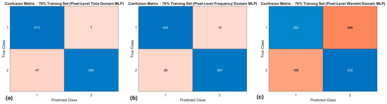
Figure 17.
Confusion matrices showing the training set performance of pixel-level NN classifiers performed on the training set: (a) time-domain, (b) frequency-domain, and (c) wavelet-domain features. True class labels are shown along the y-axis and predicted classes along the x-axis. The levels of true positive (TP) and true negative (TN) are mapped to a blue color palette, where a lighter blue color is associated with a lower level. Likewise, the levels of false positive (FP) and false negative (FN) are mapped to a red color palette, where a lighter red color is associated with a lower level.
Table 6.
NN classification performance across time, frequency, and wavelet domains, based on the training set.
4.2.2. Overview of Neural Network Testing
Figure 18 presents the confusion matrices for the pixel-level NN classifiers performed on the testing set, which is the 30% of the overall dataset, using the (a) time-domain, (b) frequency-domain, and (c) wavelet-domain features. Table 7 summarizes the pixel-level NN classification performance across time, frequency, and wavelet domains. The Macro-F1 score, accuracy, and confusion matrix elements (true positives, true negatives, false positives, and false negatives) are reported to illustrate the overall model behavior for each feature set.
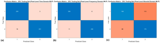
Figure 18.
Confusion matrices showing the testing set performance of pixel-level NN classifiers performed on the testing set: (a) time-domain, (b) frequency-domain, and (c) wavelet-domain features. True class labels are shown along the y-axis and predicted classes along the x-axis. The levels of true positive (TP) and true negative (TN) are mapped to a blue color palette, where a lighter blue color is associated with a lower level. Likewise, the levels of false positive (FP) and false negative (FN) are mapped to a red color palette, where a lighter red color is associated with a lower level.
Table 7.
NN classification performance across time, frequency, and wavelet domains, based on the testing set.
With the established training, validation, and testing, the following sections present further insights into the classification results for each feature domain, beginning with the time-domain.
4.2.3. Time-Domain NN Results
The NN classifier trained on the time-domain features achieved a macro-F1 score of 0.96, indicating strong performance differentiation between baseline and defect waveforms based solely on time-based features. Figure 18a shows the confusion matrix testing set at the pixel level for the time-domain NN. The results showed high, true positive and true negative rates with minimal misclassification between the classes. The results indicate that the time-domain features, despite their simplicity, capture appropriate signal variations enabling robust classification, demonstrating their importance in defect detection.
4.2.4. Frequency-Domain NN Results
The NN classifier trained on the frequency-domain features yielded the highest overall performance, achieving a macro-F1 score of 0.97, indicating an excellent performance in differentiating between the baseline and defect waveforms based solely on frequency-based features. Figure 18b shows the confusion matrix testing set at the pixel level for the frequency-domain NN. The results illustrate a strong classification capability, with even fewer misclassifications compared with the time-domain model. Frequency-domain features such as the spectral centroid, spread, and roll-off provide strong discriminative power while capturing subtle spectral shifts induced by the defects. The results validate the significance of the frequency analysis in the TTU evaluation of acoustically matched media.
4.2.5. Wavelet-Domain NN Results
In contrast to the time- and frequency-domains, NN training on the wavelet-domain features achieved a lower macro-F1 score of 0.62, indicating more difficulty in separating the baseline and defects. The confusion matrix shown in Figure 18c illustrates higher rates of misclassification relative to the time and frequency models. While wavelet decomposition captures localized time and frequency variations, the greater variability across counts and defect locations may have hindered the ability of the model to generalize when using wavelet-domain features alone. This illustrates the challenges for classification and reliance on mid-band wavelet-domain features, despite demonstrating value in the exploratory statistical analysis.
It is important to note that the wavelet-domain features in this study were implemented using a conventional first-pass approach. The db4 basis and D3 + D4 detail levels were selected based on alignment with the transducer bandwidth (centered at 5 MHz), consistent with prior ultrasonic NDE studies [13,14]. However, no optimization of the wavelet parameters or deeper feature engineering was performed in this first pass. The lower macro-F1 score (0.62) observed here reflects these factors and highlights opportunities for further refinement in future work.
4.2.6. Domain Comparison Summary
A comparison of the macro-F1 scores across domain-specific features is shown in Figure 19, where the frequency domain features provide the highest classification performance, followed closely by the time-domain features. Although the wavelet-domain features showed lower performance, they still captured meaningful localized differences between the baseline and defects.
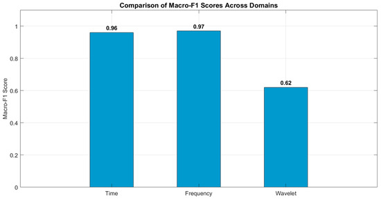
Figure 19.
Testing macro-F1 bar chart comparing scores across the time, frequency, and wavelet domains.
The results underscore the value of domain-specific feature extraction, and properly engineered feature sets classified by appropriate neural network frameworks substantially improve TTU defect detection of acoustically matched media, providing an alternative to conventional amplitude-based TTU methods. These findings confirm that domain-specific NN models, even with conventional features, can reliably detect subtle variations in acoustically matched composites, demonstrating direct applicability to industrial TTU systems where manual thresholding is insufficient.
5. Discussion
This study evaluates the use of a neural network framework for classifying acoustically matched defects in fiber-reinforced composite (FRC) laminates using through-transmission ultrasound (TTU). The NN models were independently trained using domain-specific features extracted separately from the time, frequency, and wavelet domains. The results demonstrated that both the time- and frequency-domain features enable strong defect recognition performance, achieving macro-F1 scores of 0.96 and 0.97, respectively, evaluated on an independent 30% training set. Wavelet-domain features yielded a lower macro-F1 score of 0.62, indicating more difficulty in separating the baseline from the defect conditions when using mid-band localized wavelet-domain features alone. Wavelet-domain features perhaps need machine learning methods like recurrent NNs to correctly recognize subtle time-dependent signal variations.
Time- and frequency-domain features provide signal characteristics related to amplitude, energy distribution, and spectral shifts, which proved discriminative even when acoustic impedance differences were minimized. The NN single hidden layer with ReLU activation was sufficient to model subtle nonlinear features that contributed to high classification performance. Exploratory statistical analysis confirmed that simple features evaluated alone (mean, variance, and skewness) were insufficient for accurate defect recognition across domain features that exhibited subtle changes. The results showed limited separability between the baseline and defect conditions, with the time- and frequency-domains exhibiting no statistically significant differences across ply counts. Overall, the exploratory statistical analysis emphasized that simple feature measures alone are insufficient for reliable defect detection in acoustically matched media. These findings are also consistent with prior studies showing that conventional acoustic detection methods, such as amplitude-based TTU thresholding, lack the ability to reliably detect subtle defects in acoustically matched materials, particularly when variability in ply count and material properties exceed the small impedance contrast introduced by such defects [6,9]. This further validates the need for machine learning models to capture the complex nonlinear relationships required for improved classification performance.
Although the wavelet-domain features captured localized time-frequency variations, they exhibited lower classification performance, illustrating the challenges of relying solely on mid-frequency band energy distributions without broader signal information. However, wavelet-domain features still captured meaningful localized differences between the baseline and defects and could prove to be more effective when combined with time- and frequency-domain features in future studies. This is expected, given that the wavelet-domain implementation in this study used a conventional first-pass approach. The db4 basis and D3 + D4 detail levels were selected to match the transducer bandwidth, but no parameter optimization or feature fusion was performed. Wavelet transforms often achieve better results when tuned for the specific signal characteristics or combined with other domains, as suggested. This highlights clear opportunities for future enhancement of wavelet-based classification.
The lightweight NN model architecture proved to be effective for pixel-level signal classification of ultrasound waveforms with minimal risk of overfitting. This was confirmed by a low final validation loss of approximately (0.14–0.18) across training runs.
These results demonstrate that domain feature extraction combined with NN classification can significantly improve the TTU defect detection of acoustically matched media as an alternative when conventional amplitude-based TTU methods fall short. The strong classification performance achieved across multiple ply counts further validates the potential of domain-specific AI models to aid in reliable defect detection for TTU inspections of acoustically matched media to address a key limitation of conventional manual thresholding in industrial NDE systems.
It is important to note that this study addresses the specific challenge of detecting acoustically matched foreign materials in FRC laminates. In contrast, defect types, such as porosity or delamination, which produce strong acoustic impedance mismatches, can typically be detected using standard TTU techniques without the need for machine learning classification [2].
6. Conclusions and Future Work
This study presented a novel NN classification method with domain-specific feature extraction for improved defect recognition in the TTU inspection of FRC laminates with subtle acoustically matched defects. Domain-specific features are extracted separately from the time, frequency, and wavelet domains, resulting in independent feature vectors that emphasize the signal characteristics. Independent NN classifiers were developed and evaluated, in which each waveform of each spatial TTU inspection was used as a discrete sample to obtain a larger detailed dataset of overall inspection. The NN classification performance was evaluated using the dataset that was split into 70% training and 30% testing sets. Results reveal the time- and frequency-domain features perform well, achieving macro-F1 scores of 0.96 and 0.97, respectively, while wavelet-domain features achieved lower performance scores. Wavelet-domain features perhaps need machine learning methods like recurrent NNs to correctly recognize subtle time-dependent signal variations.
These findings demonstrate the feasibility of domain-specific feature extraction combined with NN classification for acoustically matched defect recognition via TTU inspection. The use of shallow learning NN models with fully connected architectures and ReLU activation was effective in modeling the relationships inherent to the ultrasonic waveform features, providing an important capability for industrial NDE systems where traditional methods remain limited.
The method presented here is specifically intended for use in detecting subtle acoustically matched defects, such as foreign materials with near-matching impedance to the FRC base laminate, where conventional amplitude-based TTU is insufficient.
Future work will focus on expanding the dataset across more configurations to validate the generality of the machine learning model further. Additionally, the integration of time-, frequency-, and wavelet-domain features through feature fusion strategies can be explored to improve classification and robustness. Convolutional NNs (CNNs), recurrent NNs (RNNs), and spiking NNs (SNNs) with deep learning structures will be instrumental in recognizing subtle time-dependent variations in TTU signals. The wavelet transform configuration will also be optimized, including selection of alternative wavelet bases, decomposition depths, and wavelet packet analysis, as well as combining wavelet-domain features with time- and frequency-domain features to further enhance classification performances for acoustically matched materials.
Author Contributions
Conceptualization, G.L. and E.B.; methodology, G.L. and E.B.; validation, G.L.; formal analysis, G.L.; investigation, G.L.; writing—original draft preparation, G.L.; writing—review and editing, E.B.; supervision, E.B. and G.L.; and funding acquisition, G.L. and E.B. All authors have read and agreed to the published version of the manuscript.
Funding
This research received no external funding.
Data Availability Statement
The data presented in this study are available upon request.
Acknowledgments
The authors express their gratitude to the Department of Industrial Systems and Manufacturing Engineering, Wichita State University, for their administrative support.
Conflicts of Interest
The authors declare no conflict of interest.
Abbreviations
The following abbreviations are used in this manuscript:
| TTU | Through Transmission Ultrasound |
| FRC | Fiber Reinforced Composite |
| NN | Neural Network |
| NDE | Nondestructive Evaluation |
| RMS | Root Mean Square |
| FFT | Fast Fourier Transform |
| DFT | Discrete Fourier Transform |
| DWT | Discrete Wavelet Transform |
| db4 | Daubechies-4 Wavelet |
| ReLU | Rectified Linear Unit |
| CNN | Convolutional Neural Network |
| RNN | Recurrent Neural Network |
| SNN | Spiking Neural Network |
| D3 + D4 | 3rd-and-4th-Level Detail Coefficients of Wavelet |
| TP | True Positive |
| TN | True Negative |
| FP | False Positive |
| FN | False Negative |
References
- LeMay, G.; Boldsaikhan, E. Detection of Release Fabric Defects in Fiber-Reinforced Composites Using Through-Transmission Ultrasound. J. Manuf. Mater. Process. 2025, 9, 94. [Google Scholar] [CrossRef]
- LeMay, G.S.; Askari, D. A new method for ultrasonic detection of peel ply at the bondline of out-of-autoclave composite assemblies. J. Compos. Mater. 2019, 53, 245–259. [Google Scholar] [CrossRef]
- Vejdannik, M.; Sadr, A.; Albuquerque, V.H.C.; Tavares, J. Signal processing for NDE. In Handbook of Advanced Nondestructive Evaluation; Springer: Berlin/Heidelberg, Germany, 2018. [Google Scholar]
- Sopelsa Neto, N.F.; Stefenon, S.F.; Meyer, L.H.; Bruns, R.; Nied, A.; Seman, L.O.; Gonzalez, G.V.; Leithardt, V.R.Q.; Yow, K.-C. A Study of Multilayer Perceptron Networks Applied to Classification of Ceramic Insulators Using Ultrasound. Appl. Sci. 2021, 11, 1592. [Google Scholar] [CrossRef]
- Schmerr, L.W. Fundamentals of Ultrasonic Nondestructive Evaluation: A Modeling Approach; Springer: Berlin/Heidelberg, Germany, 1998. [Google Scholar]
- Rose, J.L. Ultrasonic Waves in Solid Media; Cambridge University Press: Cambridge, UK, 1999. [Google Scholar]
- Howell, P.A. (Ed.) Nondestructive Evaluation (NDE) Methods and Capabilities Handbook; NASA: Washington, DC, USA, 2020; NASA Technical Memorandum NASA/TM-2020-220568.
- Green, R.E. Non-contact ultrason techniques. Ultrasonics 2004, 42, 9–16. [Google Scholar] [CrossRef] [PubMed]
- Zhang, Z.; Li, Q.; Liu, M.; Yang, W.; Ang, Y. Through transmission ultrasonic inspection of fiber waviness for thickness-tapered composites using ultrasound non-reciprocity: Simulation and experiment. Ultrasonics 2022, 123, 106716. [Google Scholar] [CrossRef] [PubMed]
- Constantinescu, C.; Brad, R. An overview of sound features in time and frequency domain. Int. J. Adv. Stat. ITC Econ. Life Sci. 2023, 13, 45–58. [Google Scholar] [CrossRef]
- Bilgutay, N.M.; Saniie, J. Model-based approach to ultrasonic signal processing. IEEE Trans. Acoust. Speech Signal Process. 1984, 32, 396–402. [Google Scholar]
- Demirli, R.; Saniie, J. Model-based estimation of ultrasonic echoes: Part I. Analysis and algorithms. IEEE Trans. Ultrason. Ferroelectr. Freq. Control 2001, 48, 787–802. [Google Scholar] [CrossRef] [PubMed]
- Abbate, A.; Koay, J.; Frankel, J.; Schroeder, S.; Das, P. Signal detection and noise suppression using a wavelet transform signal processor. IEEE Trans. Ultrason. Ferroelectr. Freq. Control 1997, 44, 14–26. [Google Scholar] [CrossRef] [PubMed]
- Mallat, S. A Wavelet Tour of Signal Processing; Academic Press: Cambridge, MA, USA, 1999. [Google Scholar]
- Abbate, J.; Frankel, J.; Das, P. Wavelet Transform Signal Processing for Dispersion Analysis of Ultrasonic Signals. In Proceedings of the IEEE Ultrasonics Symposium, Seattle, WA, USA, 7–10 November 1995. [Google Scholar]
- Sambath, S.; Nagaraj, P.; Selvakumar, N. Automatic defect classification in ultrasonic NDT using artificial intelligence. J. Nondestruct. Eval. 2011, 30, 20–28. [Google Scholar] [CrossRef]
- Sambath, S.; Nagaraj, P.; Selvakumar, N.; Arunachalam, S.; Page, T. Automatic detection of defects in ultrasonic testing using artificial neural network. Int. J. Microstruct. Mater. Prop. 2010, 5, 561–574. [Google Scholar] [CrossRef]
- Boldsaikhan, E.; Corwin, E.; Logar, A.; Arbegast, W. Neural Network Evaluation of Weld Quality using FSW Feedback Data. In Proceedings of the 6th International Friction Stir Welding Symposium, Saint-Sauveur, Nr Montreal, Canada, 10–12 October 2006. [Google Scholar]
- Chen, D.; Zhou, Y.; Wang, W.; Zhang, Y.; Deng, Y. Ultrasonic signal classification and porosity testing for CFRP materials via artificial neural network. Mater. Today Commun. 2022, 30, 103021. [Google Scholar] [CrossRef]
- Huang, M.; Liu, J.; Tang, H. Deep neural network-based defect detection using air-coupled through-transmission ultrasound. J. Nondestruct. Eval. 2023, 42, 43. [Google Scholar] [CrossRef]
- Smith, S.W. The Scientist and Engineer’s Guide to Digital Signal Processing; California Technical Publishing: San Diego, CA, USA, 1997. [Google Scholar]
- Oppenheim, A.V.; Schafer, R.W. Discrete-Time Signal Processing, 3rd ed.; Pearson: London, UK, 2009. [Google Scholar]
- Boldsaikhan, E.; Corwin, E.M.; Logar, A.M.; Arbegast, W.J. The use of neural network and discrete Fourier transform for real-time evaluation of friction stir welding. Applied Soft Computing. 2011, 11, 4839–4846. [Google Scholar] [CrossRef]
- Kim, J.-G.; Jang, C.; Kang, S.-S. Classification of ultrasonic signals of thermally aged cast austenitic stainless steel (CASS) using machine learning (ML) models. Nucl. Eng. Technol. 2022, 54, 1167–1174. [Google Scholar] [CrossRef]
- Meduri, S. Activation functions in neural networks: A comprehensive overview. Int. J. Res. Comput. Appl. Inf. Technol. 2024, 7, 2. [Google Scholar]


Disclaimer/Publisher’s Note: The statements, opinions and data contained in all publications are solely those of the individual author(s) and contributor(s) and not of MDPI and/or the editor(s). MDPI and/or the editor(s) disclaim responsibility for any injury to people or property resulting from any ideas, methods, instructions or products referred to in the content. |
© 2025 by the authors. Licensee MDPI, Basel, Switzerland. This article is an open access article distributed under the terms and conditions of the Creative Commons Attribution (CC BY) license (https://creativecommons.org/licenses/by/4.0/).