Flexible Job Shop Scheduling with Job Precedence Constraints: A Deep Reinforcement Learning Approach

Abstract

The flexible job shop scheduling problem with job precedence constraints (FJSP-JPC) is highly relevant in industrial production scenarios involving assembly operations. Traditional methods, such as mathematical programming and meta-heuristics, often struggle with scalability and efficiency when solving large instances. We propose a deep reinforcement learning (DRL) approach to minimize makespan in FJSP-JPC. The proposed method employs a heterogeneous disjunctive graph to represent the system state and a multi-head graph attention network for feature extraction. An actor–critic framework, trained using proximal policy optimization (PPO), is adopted to make operation sequencing and machine assignment decisions. The effectiveness of the proposed method is validated through comparisons with several classic dispatching rules and a state-of-the-art DRL approach. Additionally, the contributions of key mechanisms, such as information diffusion, node features, and action space, are analyzed through a full factorial design of experiments.

1. Introduction

The flexible job shop scheduling problem (FJSP) is an important challenge widely faced in manufacturing industries. In contrast to the classic scheduling problem (JSP), operations in FJSP can be processed on a set of eligible machines. Additionally, the job precedence constraint (JPC) is another practical feature that often exists in various types of production scenarios. More specifically, the JPC indicates that some jobs can start processing after one or several other jobs have been completed. That is, the precedence relationship exists not only among operations in the job as in classic job shop scheduling, but also among different jobs.

An example of the JPC is shown in Figure 1. In this figure, each job (rectangle) represents an item, which could be either a product or a component, and each operation (circle) corresponds to a manufacturing process for that item. Edges indicate precedence relationships between operations or jobs. In this example, $J_6$ is the final product, and operation $O_{6,1}$ represents its final assembly. The components of $J_6$ include $J_1$, $J_2$, and $J_5$, while $J_2$ itself is composed of parts $J_3$ and $J_4$. These hierarchical assembly relationships form a strict tree-like structure among the jobs, similar to a Bill of Materials (BOM).

Several methodologies have been proposed to solve FJSP [1]. One of the most important is mathematical programming, including mixed integer linear programming (MILP) [2,3] and constraint programming [4]. Yet, due to the NP-hardness of FJSP, the direct solving of these models tends to be difficult even for medium-scale instances [5]. Recent works for FJSP have focused on meta-heuristic algorithms, including genetic algorithm [6], Grey Wolf Algorithm [7], particle swarm optimization [8], etc. Li and Gao [9] proposed a method combining the population-based global search of genetic algorithm with the local improvement of tabu search, achieving a higher solution performance and shorter computational time for FJSP. Xie et al. [10] proposed a hybrid algorithm for the distributed FJSP that combines the global search capability of genetic algorithms with the local search strength of tabu search. He et al. [11] developed a method based on the ant colony optimization algorithm, incorporating heuristic rules to address both scheduling and transportation tasks in the FJSP.

Although traditional operations research methods can generally produce promising results, they often involve complex and time-consuming processes. Their computational burden grows rapidly with problem size, making them less suitable for dynamic environments where quick decision-making is essential. To balance computational cost and solution quality, recent research in JSP and FJSP has increasingly shifted toward artificial intelligence approaches, including reinforcement learning (RL) [12] and deep reinforcement learning (DRL) [13]. DRL, in particular, leverages neural networks to map environmental information to optimal decision actions [14]. Johnson et al. [15] proposed a multi-agent reinforcement learning (MARL) method for solving real-time FJSP in robotic assembly cells, demonstrating high flexibility and efficiency in dynamic environments. Luo et al. [16] introduced a hierarchical multi-agent method based on proximal policy optimization (PPO), tailored for real-time scheduling in discrete flexible manufacturing systems. Du et al. [17] studied a multi-objective FJSP with crane transportation and preparation time constraints. They developed a double deep Q-network algorithm with a specialized network architecture to minimize both makespan and total energy consumption. Han and Yang [18] proposed an end-to-end DRL framework based on the 3D disjunctive graph and an improved pointer network, which integrates both static and dynamic features for FJSP. Xu et al. [19] developed a scheduling framework based on the transformer and PPO for FJSP, which captures the relationships between state features and enhances performance through composite dispatching rules and a dense reward function.

These DRL methods rely on manually designed environmental features, which may overlook important information and struggle to handle the complex constraint relationships between operations and machines. To address this limitation, Graph Neural Networks (GNNs) have gradually been applied to FJSP. By representing operations, machines, and constraints as a graph structure, GNNs can effectively capture the structural characteristics of scheduling problems [20]. Park et al. [21] proposed a GNN-PPO framework for solving JSP, which models the problem structure using graphs and demonstrates strong generalization capabilities across untrained datasets of varying sizes. Song et al. [22] developed an end-to-end approach based on GNN and PPO for FJSP, employing a heterogeneous graph to capture the complex relationships between operations and machines. Wang et al. [23] proposed a DRL framework based on a dual attention network and PPO for FJSP. It constructs attention blocks for operation messages and machine messages to accurately represent their interconnections and performs well on large-scale instances. Lei et al. [24] introduced an end-to-end DRL framework for FJSP, utilizing disjunctive graphs to represent the local system state and designing a multi-action PPO algorithm that learns job and machine action policies, effectively handling instances of various sizes.

Besides the aforementioned studies, relatively few works have addressed the FJSP with job precedence constraints. Xiong et al. [25] proposed novel scheduling rules that account for job tardiness in addressing dynamic job shop scheduling problems with job batch releases and extended technological precedence constraints. Zhu and Zhou [26] investigated a job shop scheduling problem with job precedence constraints for bicycle assembly and proposed a multi-micro-swarm leadership hierarchy-based optimization algorithm to address this problem. Zhang et al. [27] studied the FJSP with multi-level assembly structures and proposed a distributed ant colony optimization algorithm to optimize makespan and total tardiness. Lin et al. [28] introduced the FJSP with job precedence constraints accommodating both machining and assembly operations, designing a genetic algorithm with an innovative two-dimensional encoding method to solve it.

Table 1. Existing methods for the job shop scheduling problem.

Research	State	Algorithm	Objective	Problem	Special Constraint
Li and Gao [9]	-	GA, TS	Makespan	FJSP
Xie et al. [10]	-	GA, TS	Makespan	FJSP
He et al. [11]	-	ACO	Makespan	FJSP	Transportation
Johnson et al. [15]	Vector	DDQN	Makespan	FJSP
Luo et al. [16]	Vector	PPO	Total tardiness, machine utilization, machine workload	FJSP	Partial-no-wait constraints
Du et al. [17]	Vector	DDQN	makespan, total energy consumption	FJSP	Transportation, preparation time
Luo [13]	Vector	DDQN	Total tradiness	FJSP
Han and Yang [18]	Vector	REINFORCE	Makespan	FJSP
Xu et al. [19]	Vector	PPO	Makespan	FJSP
Park et al. [21]	Disjunctive graph	PPO	Makespan	JSP
Song et al. [22]	Disjunctive graph	PPO	Makespan	FJSP
Wang et al. [23]	Disjunctive graph	PPO	Makespan	FJSP
Lei et al. [24]	Disjunctive graph	PPO	Makespan	FJSP
Xiong et al. [25]	-	PDRs	Total tardiness, tardy jobs rate	JSP	Technological precedence constraints
Zhu and Zhou [26]	-	M2SLHO	Makespan	FJSP	Job precedence constraints
Zhang et al. [27]	-	ACO	Makespan, total tardiness, total workload	FJSP	Job precedence constraints
Lin et al. [28]	-	GA	Makespan	FJSP	Job precedence constraints
This paper	Disjunctive graph	PPO	Makespan	FJSP	Job precedence constraints

summarizes some recent works mentioned above on the job shop scheduling problem and compares the differences between our method and them. In summary, most current methods for the FJSP-JPC are based on mathematical programming and metaheuristic algorithms, which may struggle to adapt to dynamic scenarios due to their relatively long computational times. DRL-based methods, on the other hand, demonstrate significant potential for improving the resolution efficiency while maintaining the solution quality. However, to the best of our knowledge, no DRL-based approach has yet been proposed for FJSP-JPC. To fill this gap, this paper investigates the FJSP-JPC with the objective of minimizing makespan. The main contributions of this paper are as follows:

1.

We formulate the FJSP-JPC as a MILP model and develop a heterogeneous disjunctive graph model for improving problem representation.

2.

We propose a DRL-based approach to solve the FJSP-JPC, which outperforms traditional priority dispatching rules (PDRs) as well as a state-of-the-art DRL-based method.

3.

We analyze the impact of various factors in the proposed DRL framework, such as node embeddings, information diffusion range, and action space selection, on the algorithm performance.

The remainder of this paper is organized as follows. Section 2 provides the definition and mathematical model of FJSP-JPC. Section 3 introduces the proposed method. Section 4 reports the experimental results. Section 6 concludes this paper.

2. Problem Formulation

2.1. Problem Description

A set of n jobs $\mathit{J}=\{J_1,J_2,\dots ,J_n\}$ are to be processed by a set of m machines $\mathit{M}=\{M_1,M_2,\dots ,M_m\}$ in the job shop. Each job $J_i\in \mathit{J}$ consists of a set of $n_i$ consecutive operations $\{O_{i1},O_{i2},\dots ,O_{i{n}_i}\}$. Each operation, say $O_{ij}$, can be processed by a machine k selected from the eligible subset ${\mathit{M}}_{\mathit{ij}}\subseteq \mathit{M}$ with a processing time $p_{ijk}$.

In accordance with the process routing, there are precedence constraints among the jobs. Let ${\mathit{P}}_{\mathit{i}}$ be the set of precedent jobs for job $J_i$, meaning that $J_i$ can start processing only after all the jobs in ${\mathit{P}}_{\mathit{i}}$ are completed. Note that ${\mathit{P}}_{\mathit{i}}$ could be empty. The objective of the FJSP-JPC is to minimize the makespan $C_{max}$. Makespan is defined as the total time span from the initiation of the first operation to the completion of the last operation. Other characteristics of the problem are as follows.

1.

Each machine can process at most one operation at a time.

2.

Machines are reliable, and no breakdowns can occur.

3.

Machine setup times are included in the processing times.

4.

Transportation between machines is not considered.

2.2. Mathematical Programming Model

In this section, we formulate the problem using a MILP model as follows.

2.2.1. Parameters

• n: total number of jobs.
• m: total number of machines.
• $\mathit{J}$: set of jobs.
• $\mathit{M}$: set of machines.
• $J_i$: the ith job, $1⩽i⩽n$.
• $M_k$: the kth machine, $1⩽k⩽m$.
• $n_i$: total number of operations belonging to job $J_i$.
• $O_{ij}$: the jth operation of job $J_i$, $1⩽j⩽n_i$.
• ${\mathit{M}}_{\mathit{ij}}$: set of eligible machines that can process operation $O_{ij}$, ${\mathit{M}}_{\mathit{ij}}\subseteq \mathit{M}$.
• $p_{ijk}$: processing time of operation $O_{ij}$ on machine $M_k$.
• ${\mathit{P}}_{\mathit{i}}$: set of precedent jobs for job $J_i$.
• H: a large number.

2.2.2. Decision Variables

• ${\alpha }_{ijk}$: 1 if $O_{ij}$ is assigned to machine $M_k$; 0 otherwise.
• ${\beta }_{iji\prime j\prime }$: 1 if $O_{ij}$ is scheduled before $O_{i\prime j\prime }$; 0 otherwise.
• $s{t}_{ij}$: starting time of operation $O_{ij}$.
• $C_{max}$: makespan of the entire production process.

2.2.3. Objective and Constraints

$$min{C}_{max}$$

(1)

$$\sum _{k\in {\mathbf{M}}_{\mathbf{ij}}}{\mathit{\alpha }}_{ijk}=1,\forall 1⩽i⩽n,1⩽j⩽n_i$$

(2)

$$s{t}_{ij}⩾s{t}_{i(j-1)}+\sum _{k\in {\mathbf{M}}_{\mathbf{i}(\mathbf{j}-\mathbf{1})}}{\mathit{\alpha }}_{i(j-1)k}{p}_{i(j-1)k},\forall i,j$$

(3)

$$\begin{array}{cc}\hfill & s{t}_{ij}⩾s{t}_{i\prime j\prime }+p_{i\prime j\prime k}-(2-{\mathit{\alpha }}_{ijk}-{\alpha }_{i\prime j\prime k}+{\beta }_{iji\prime j\prime })H\hfill \\ \hfill & \forall i,i\prime ,j,j\prime ,(i,j)\ne (i\prime ,j\prime ),k\in {\mathit{M}}_{\mathit{ij}}\cap {\mathit{M}}_{\mathit{i}\prime \mathit{j}\prime }\hfill \end{array}$$

(4)

$$\begin{array}{cc}\hfill & s{t}_{i\prime j\prime }⩾s{t}_{ij}+p_{ijk}-(3-{\alpha }_{ijk}-{\alpha }_{i\prime j\prime k}-{\mathit{\beta }}_{iji\prime j\prime })H\hfill \\ \hfill & \forall i,i\prime ,j,j\prime ,(i,j)\ne (i\prime ,j\prime ),k\in {\mathit{M}}_{\mathit{ij}}\cap {\mathit{M}}_{\mathit{i}\prime \mathit{j}\prime }\hfill \end{array}$$

(5)

$$C_{max}⩾s{t}_{i{n}_i}+\sum _{k\in {\mathit{M}}_{\mathit{i}{\mathit{n}}_{\mathit{i}}}}{p}_{i{n}_{i}k}{\alpha }_{i{n}_{i}k},\forall i$$

(6)

$$s{t}_{i1}⩾s{t}_{i\prime n_{i\prime }}+\sum _{k\in {\mathit{M}}_{\mathit{i}\prime {\mathit{n}}_{\mathit{i}\prime }}}{p}_{i\prime n_{i\prime }k}{\mathit{\alpha }}_{i\prime n_{i\prime }k},\forall i,i\prime \in {\mathit{P}}_{\mathit{i}}$$

(7)

$${\mathit{\alpha }}_{ijk}\in \left\{0,1\right\},\forall i,j,k\in {\mathit{M}}_{\mathit{ij}}$$

(8)

$${\mathit{\beta }}_{iji\prime j\prime }\in \left\{0,1\right\},\forall i,j,i\prime ,j\prime$$

(9)

The objective (1) is to minimize the makespan $C_{max}$. Constraint (2) ensures that each operation must be assigned to one eligible machine. Constraint (3) ensures that an operation can start after the completion of its predecessor in the same job. Constraints (4) and (5) together ensure that two distinct operations, $O_{ij}$ and $O_{i\prime j\prime }$, assigned to the same machine $M_k$, do not overlap in processing time and adhere to the precedence order determined by ${\beta }_{iji\prime j\prime }$. Constraint (6) defines the makespan. Constraint (7) ensures that a job cannot start until all its precedent jobs have been completed.

3. Methodology

FJSP-JPC involves two types of decisions: assigning an operation to one of its eligible machines, and sequencing the operations on the same machine. Though FJSP-JPC is a combinatorial optimization problem, the schedule construction can be viewed as a sequential decision-making procedure. This allows for the possibility to formulate the schedule procedure as a Markov decision process (MDP), where the optimal policy can be estimated by RL algorithms. In this section, the details of our proposed approach are presented. Firstly, we explain the scheduling environment for FJSP-JPC. Then, the definitions of state, action, reward function, and state transition logic are described, along with several improvement strategies we propose.

3.1. MDP Formulation of the Scheduling Problem

At the first scheduling step ($t=1$), the system clock is initialized to $T=0$, with all machines idle and all operations unscheduled. Let $s_t$ denote the current system state. Based on $s_t$, the agent takes an action $a_t$, which involves selecting an unscheduled operation and scheduling its start time on one of its eligible machines. This action transitions the system to a new state $s_{t+1}$, and the environment provides a reward $r_t$.

Typically, only a subset of operations can be scheduled at time T, such as those whose predecessors have been completed [23]. However, the definition of this subset is not unique. If no such operations are available, or all machines that can process these operations are busy, the system clock advances to the earliest time at which a machine completes a scheduled operation. An operation is considered completed once its scheduled completion time is earlier than the system clock. This process continues until all operations have been scheduled and completed.

3.2. State

The state representation of FJSP typically summarizes the environment information at time T. Traditional methods often use manually crafted features, such as job completion rate and machine load rate, as state descriptors [13]. The advantage of this approach lies in its ability to abstract information into fixed-size feature vectors, making it applicable to systems of different scales and allowing the agent a certain degree of generalization capability. However, the limitations of this method are also evident. In principle, the state representation provided to the agent should comprehensively capture all of the relevant information about the environment at time T. In practice, the complexity of manufacturing systems makes it difficult for manually designed features to include all critical aspects. Important factors such as job precedence constraints and machine-operation compatibility may be overlooked. To address this issue and better capture the complex characteristics of the environment, we propose a state representation method based on a heterogeneous disjunctive graph, combined with a multi-head graph attention network (GAT), to learn rich and structured features automatically.

3.2.1. Heterogeneous Disjunctive Graph

The disjunctive graph is a graph model used to represent the scheduling process of JSP [29]. The typical disjunctive graph is a directed acyclic graph written as $\mathbf{G}=(\mathbf{O},\mathbf{A},\mathbf{E})$. Here, $\mathbf{O}=\left\{O_{ij}\mid \forall i,j\right\}\cup \left\{Start,End\right\}$ is the set of nodes consisting of all operations and two dummy operations representing the start and end of processing. $\mathbf{A}$ is the set of directed conjunctive arcs, representing the precedence relationship between operations. $\mathbf{E}$ is the set of disjunctive arcs connecting the operations that can be processed on the same machine $M_k$. Solving JSP involves fixing the direction of each disjunctive arc and, thus, arranging the sequence of operations on the same machine.

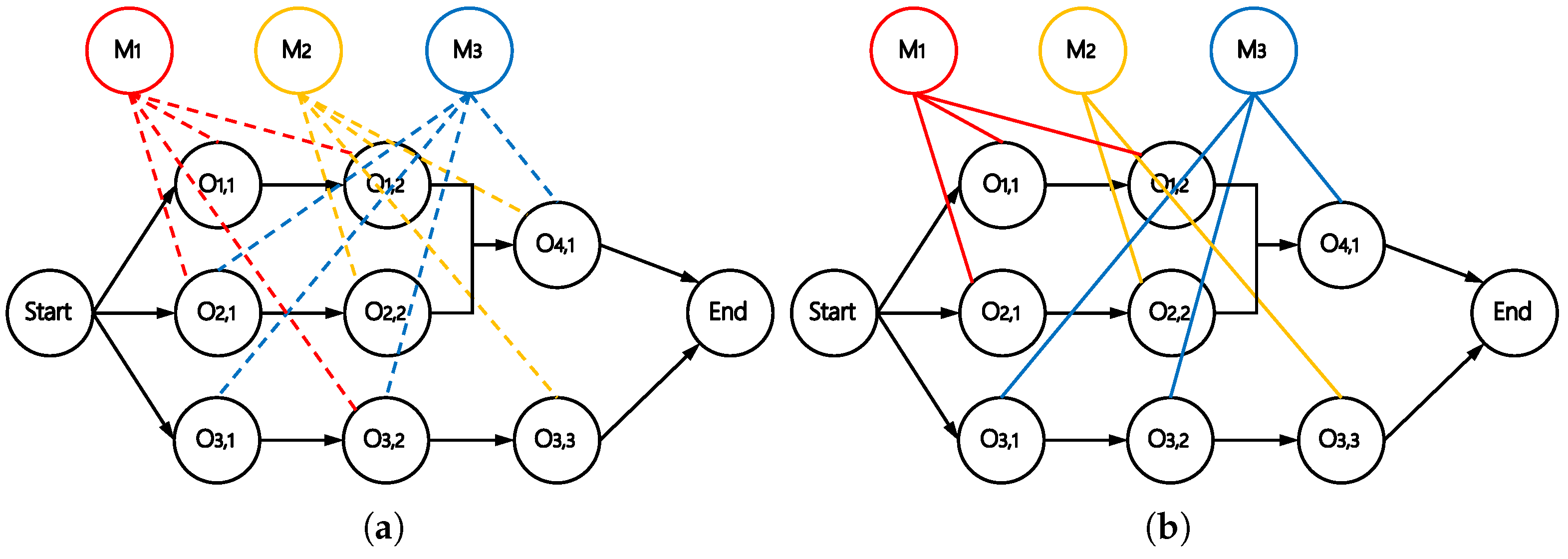
Unlike JSP, each operation in FJSP can have more than one eligible machines. To better represent this relationship between operations and machines, a heterogeneous disjunctive graph $\mathbf{H}=(\mathbf{O},\mathbf{M},\mathbf{A},\mathbf{D})$ is designed. As shown in Figure 2a, the graph retains operation nodes $\mathbf{O}$ and directed conjunctive arcs $\mathbf{A}$, while introducing a new type of node, i.e., machine nodes $\mathbf{M}$, to represent the machines. The disjunctive arcs $\mathbf{D}$ build connections between the operations and their eligible machines.

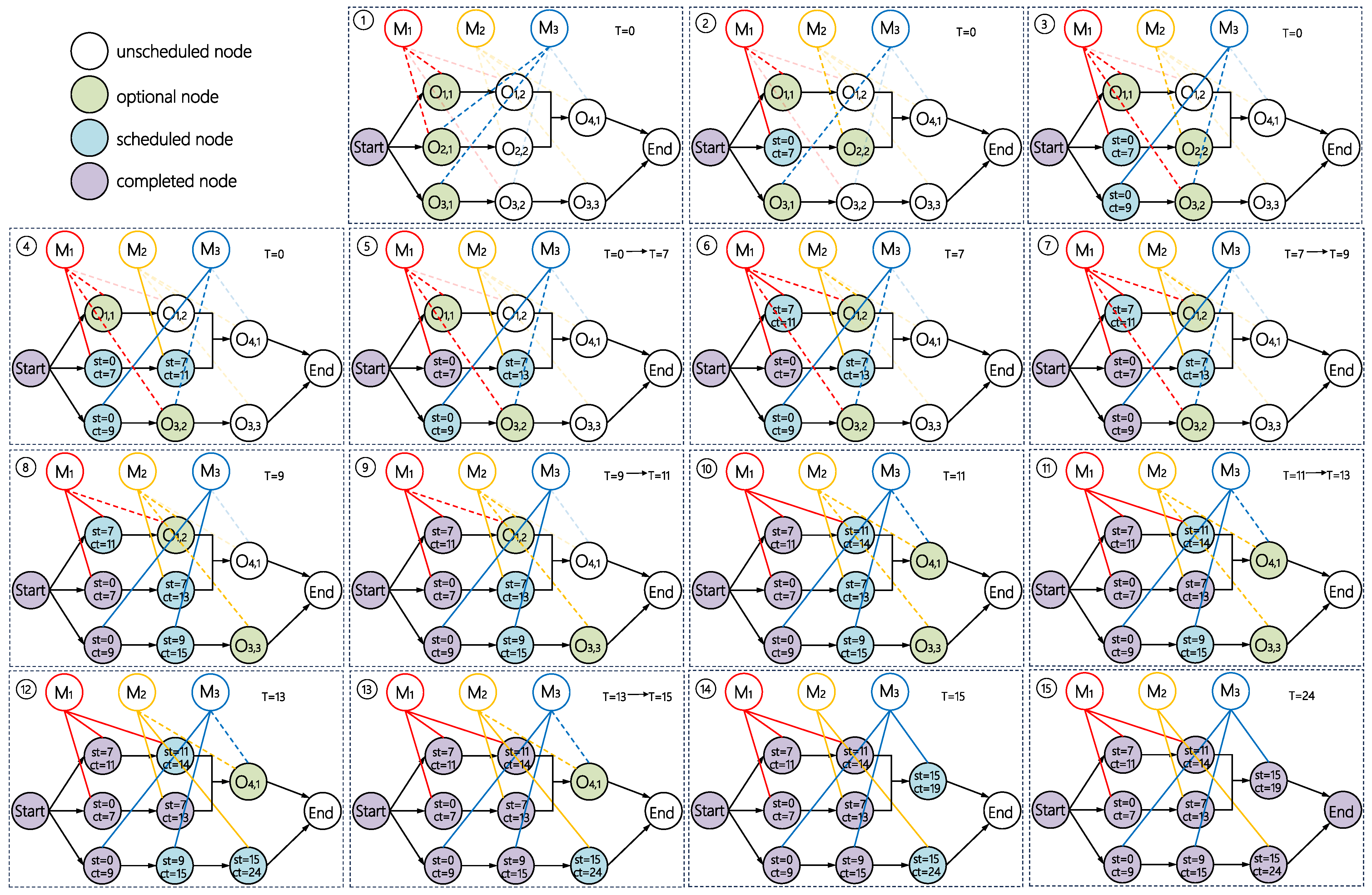
The scheduling process involves selecting one disjunctive arc for each operation node, converting it into a conjunctive arc, and determining the operation start time, which is stored in the node features. A possible solution is illustrated in Figure 2b. The detailed step-by-step scheduling procedure can be found in Appendix A.

We embed a set of features into the graph to represent scheduling information.

Table 2. Features for operation nodes, machine nodes, and undirected arcs.

ID	Description
Features of operation node $O_{ij}$
(o1)	Scheduling flag: 0 if $O_{ij}$ is unscheduled; otherwise, 1.
(o2)	Estimated completion time (see Equation (20)).
(o3)	Minimum processing time among all machines.
(o4)	Span of processing time among all machines.
(o5)	Average processing time among all machines.
(o6)	Waiting time: The time elapsed since the ready time of $O_{ij}$ until the current time T.
(o7)	Remaining processing time: From T to estimated completion time (0 if unscheduled).
(o8)	Number of remaining operations from $O_{ij}$ to End.
(o9)	Remaining work: Sum of average processing times of unscheduled operations from $O_{ij}$ to End.
(o10)	Number of machines that $O_{ij}$ can be processed on.
Features of machine node $M_k$
(m1)	Number of candidate operations that $M_k$ can process.
(m2)	Number of unscheduled operations that $M_k$ can process.
(m3)	Minimum processing time of operations that $M_k$ can process.
(m4)	Average processing time of operations that $M_k$ can process.
(m5)	Waiting time: The time elapsed since the machine $M_k$ became free until the current time T.
(m6)	Remaining processing time: The duration from the current time T until $M_k$ becomes free (0 if $M_k$ is free).
(m7)	Free time: The moment when $M_k$ is free.
(m8)	Working flag: 0 if $M_k$ is free; otherwise, 1.
Features of undirected arc $(O_{ij},M_k)$
(a1)	Processing time $p_{ijk}$.
(a2)	Ratio of $p_{ijk}$ to the maximum processing time of $O_{ij}$.
(a3)	Ratio of $p_{ijk}$ to the maximum processing time of candidate operations that $M_k$ can process at the current time.
(a4)	Ratio of $p_{ijk}$ to the maximum processing time of unscheduled operations.
(a5)	Ratio of $p_{ijk}$ to the maximum processing time of unscheduled operations that $M_k$ can process.
(a6)	Ratio of $p_{ijk}$ to the maximum processing time of all feasible $\left(O_{ij},M_k\right)$.
(a7)	Ratio of $p_{ijk}$ to the remaining work of $O_{ij}$.
(a8)	Summation of the “Waiting time” feature of $O_{ij}$ and $M_k$.

reports the features for each operation node in $\mathbf{O}$, machine node in $\mathbf{O}$, and undirected arc in $\mathbf{D}$. Most of these features are identical to those used in [23] for FJSP; we modify a subset of them to accommodate the JPC characteristics of our problem.

More specifically, compared to those proposed in Wang et al. [23], the newly designed features are (o2), (o8), (o9), and (a3). These features are specifically adapted to the tree-like JPC in our problem. More specifically, when computing the estimated completion time of operation $O_{ij}$ in (o2), we consider all operations related to $O_{ij}$ through JPC across the entire graph. Instead of assuming $C_{i0}=0$, we determine the estimated starting time of $C_{i0}$ by Equation (20). Similarly, when calculating the number of remaining operations (o8) and the remaining work (o9), we account for all operations connected to $O_{ij}$ via JPC, i.e., all unscheduled operations along the directed path from $O_{ij}$ to End. On the other hand, the calculation of feature (a3) differs from that in Wang et al. [23]. Since we use a different action space, the set of candidate operations that a machine, say $M_k$, can process at a given time T is larger than that in the original version.

3.2.2. Multi-Head GAT

Traditional neural network architectures, such as the multi-layer perceptron (MLP), can only process inputs with fixed-size dimensions. However, in FJSP-JPC, the size of the graph structures representing the states varies between instances. To tackle this difficulty, we utilize a multi-head GAT to process the graph features. The multi-head GAT uses a graph of arbitrary size as input and outputs a graph of the same topology with updated feature vectors in each node and arc. The GAT assigns different attention weights to neighboring nodes, allowing it to focus more on important neighbors during the feature aggregation process. Meanwhile, the graph attention layer utilizes attention mechanism to learn critical structural features of the graph during the embedding process and places greater emphasis on the local information by applying attention masks. The attention mechanism is described in the following subsection.

3.2.3. Attention Mechanism

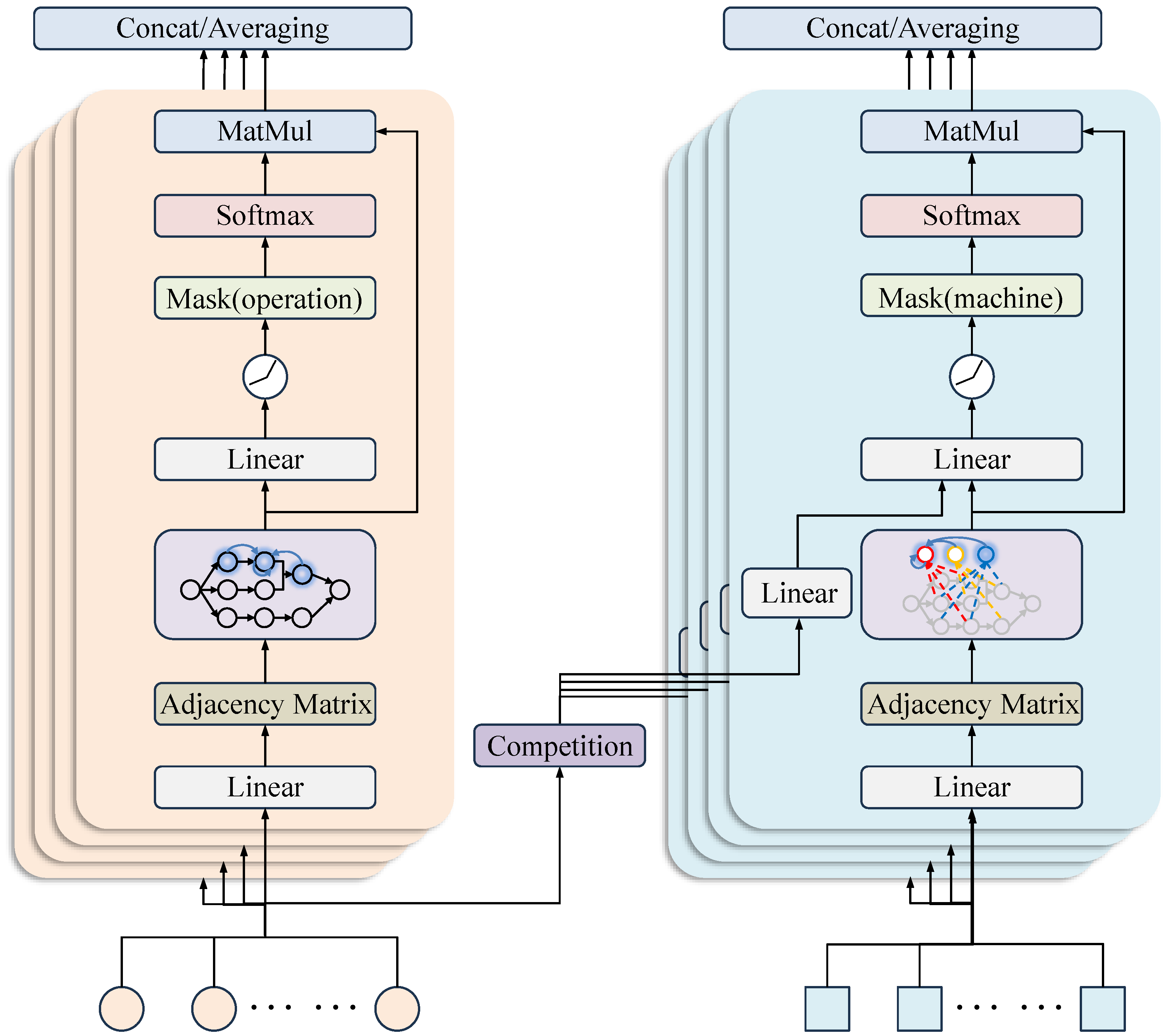
The heterogeneous disjunctive graph can essentially be viewed as a superposition of two distinct subgraphs, i.e., the operation relationship graph and the machine relationship graph. Hence, two separate attention blocks are employed in the model to embed the features of operations and machines, respectively. This design facilitates the learning of complex connections both between operation nodes and between operation nodes and machine nodes. While the two attention blocks share similar structural designs, they have different dimensions and parameters.

Operation attention block. The inputs to this block are the features of the operation nodes. The precedence constraints between operation nodes are represented by an adjacency matrix, which is used to propagate information between nodes with strong correlations. Specifically, each operation $O_{ij}\in \mathbb{O}$ is associated with an input feature $h_{O_{ij}}$. Let ${\mathcal{N}}_{ij}$ denote the set of direct predecessor and successor nodes that are less than one edge away from $O_{ij}$, including $O_{ij}$ itself. Notably, ${\mathcal{N}}_{ij}$ may also include cross-job operations that do not belong to the same job as $O_{ij}$. For example, in Figure 3a, the operation node $O_{41}$ aggregates information from two of its predecessors in different jobs, namely $O_{12}$ and $O_{22}$. This mechanism enables information to diffuse across the graph, enhancing overall performance.

The methodology for computing the attention coefficient between $O_{ij}$ and $O_{i\prime j\prime }$ is as follows:

$$\begin{array}{cc}\hfill e_{iji\prime j\prime }^o& =\mathrm{LeakyReLU}\left({\overrightarrow{\mathrm{a}}}^{\top }\left[\left(\mathbf{W}{h}_{O_{ij}}\right)\parallel \left(\mathbf{W}{h}_{O_{i\prime j\prime }}\right)\right]\right),\hfill \\ \hfill & \forall O_{i\prime j\prime }\in {\mathcal{N}}_{ij},\hfill \end{array}$$

(10)

where $\mathbf{W}\in {\mathbb{R}}^{d_o^{\prime }\times d_o}$ is a linear transformation that projects the node features $h_{O_{ij}}$ and $h_{O_{i\prime j\prime }}$ into a higher-dimensional space. The transformed features are concatenated and then passed through a single-layer feedforward neural network with a $\mathrm{LeakyReLU}$ activation function. The network weights are denoted by $\overrightarrow{\mathrm{a}}\in {\mathbb{R}}^{2d_o^{\prime }}$. Afterwards, we normalize attention coefficients by the softmax function as follows:

$$\begin{array}{cc}\hfill {\mu }_{iji\prime j\prime }^o& =\mathrm{Softmax}\left(e_{iji\prime j\prime }^o\right)\hfill \\ \hfill & ={\displaystyle \frac{exp\left(e_{ij}\right)}{{\sum }_{O_{i\prime j\prime }\in {\mathcal{N}}_{ij}\setminus {\mathcal{U}}_{ij}}exp\left(e_{i\prime j\prime }\right)}},\forall O_{ij}\in {\mathcal{N}}_{ij}.\hfill \end{array}$$

(11)

where ${\mathcal{U}}_{ij}$ represents the set of completed and dummy operation nodes whose effect on the scheduling process is not considered. Having the attention coefficients, we update the features for each operation node by

$$h_{O_{ij}}^{\prime }=\mathrm{ELU}\left(\sum _{O_{i\prime j\prime }\in {\mathcal{N}}_{ij}}{\mu }_{iji\prime j\prime }^o\mathbf{W}{h}_{O_{ij}}\right),$$

(12)

where $\mathrm{ELU}$ is the exponential linear unit nonlinear activation function.

This approach updates the node embeddings by aggregating information from their neighbors. Let $h_{O_{ij}}^{\left(l\right)}$ represent the node embedding after passing through l attention layers. By doing so, $h_{O_{ij}}^{\left(l\right)}$ incorporates information from a broader range of nodes, thereby expanding the receptive field.

Machine attention block. The attention block for machines is similar to that for operations; the difference is in the consideration of neighbors. In FJSP, machines are related to each other due to the competition of unscheduled operations. More specifically, if an unscheduled operation can be processed by two machines, say $M_k$ and $M_{k\prime }$, there can be a competitive relationship between them. As shown in Figure 3b, $M_1$ is related to $M_2$ through the competition for $O_{12}$, while it is related to $M_3$ by the competition for $O_{21}$ and $O_{32}$. Let ${\mathcal{C}}_{kk\prime }$ be the set of operations that $M_k$ and $M_{k\prime }$ compete for, and ${\mathcal{N}}_k$ be the set of machines competing with machine $M_k$ (including $M_k$ itself). The parameter that measures the competitive intensity between $M_k$ and $M_{k\prime }$ can be defined as follows:

$${\kappa }_{kk\prime }=\sum _{O_{ij}\in {\mathcal{C}}_{kk\prime }}{h}_{O_{ij}}.$$

(13)

Then, the attention coefficient between machines $M_k$ and $M_{k\prime }$ can be computed by

$$\begin{array}{cc}\hfill e_{kk\prime }^m=& \mathrm{LeakyReLU}\hfill \\ \hfill & \left({\overrightarrow{\mathrm{b}}}^{\top }\left[\left(\mathbf{P}{h}_{M_k}\right)\parallel \left(\mathbf{P}{h}_{M_{k\prime }}\right)\parallel \left(\mathbf{Q}{\kappa }_{kk\prime }\right)\right]\right),\hfill \\ \hfill & \forall M_k,M_{k\prime }\in {\mathcal{N}}_k.\hfill \end{array}$$

(14)

where $\mathbf{P}\in {\mathbb{R}}^{d_m^{\prime }\times d_m}$ is a linear transformation scaling up the machine features vectors, and $\mathbf{Q}$ is a matrix evaluating the influence of a competitive intensity on non-self-attention. Specifically, if ${\mathcal{C}}_{kk\prime }$ is empty, $M_k$ and $M_{k\prime }$ do not affect each other, and the attention coefficients between them are set to zero by a mask. Finally, we update the machine features $h_{M_k}$ by

$${\mu }_{kk\prime }^m=\mathrm{Softmax}\left(e_{kk\prime }^m\right),$$

(15)

$$h_{M_k}^{\prime }=\mathrm{ELU}\left(\sum _{M_k\in {\mathcal{N}}_k}{\mu }_k^m\mathbf{P}{h}_{M_k}\right).$$

(16)

3.2.4. Multi-Head Attention

According to Vaswani et al. [30], the expressive power of the attention mechanism can be enhanced by capturing information across different dimensions using multiple independent attention heads. To leverage this, we employ $\mathcal{H}$ attention heads within both the operation and machine attention block. More specifically, each head uses the same raw features of operation nodes (or machine nodes) as inputs, while the attention coefficients ${\mu }_{iji\prime j\prime }^o$s (or ${\mu }_{kk\prime }^m$s) are computed in parallel and independently. Then, the outputs of each head are combined by an aggregation operator. Following GAT, we use concatenation except for the last attention layer, which is combined by an averaging operator.

3.2.5. Global Average Pooling

Besides the node features, we apply an average pooling on all the active nodes to obtain a global feature vector $h_{g_t}^{\left(l\right)}$ describing the overall state of the graph, which is given by

$$h_{g_t}^{\left(l\right)}=\left[\left({\displaystyle \frac{1}{\left|𝒪\right|}}\sum _{O_{ij}\in 𝒪}{h}_{O_{ij}}^{\left(l\right)}\right)\parallel \left({\displaystyle \frac{1}{\left|\mathcal{M}\right|}}\sum _{M_k\in \mathcal{M}}{h}_{M_k}^{\left(l\right)}\right)\right].$$

(17)

3.2.6. The Overall Architecture

The overall architecture of the multi-head GAT is illustrated in Figure 4. The input consists of features of nodes and operation–machine arcs. After passing through the attention layers, the node features are updated. The output is a graph with the same structure but with updated features, which serve as the state to guide scheduling decisions.

3.3. Action

In prior studies on DRL-based FJSP [13], priority dispatching rules (PDRs) are often employed as actions for decision-making. However, this action space, derived from human experience, while capable of quickly generating suboptimal solutions, fails to fully encompass all feasible actions in $s_t$, potentially resulting in performance limitations.

To maintain the degree of exploration, we define the action set ${\mathcal{A}}_t$ as all feasible operation–machine pairs that can be selected at step t. A similar approach is adopted in [31]. More specifically, an operation–machine pair $(O_{ij},M_k)$ is feasible at step t when $O_{ij}$ is unscheduled and all its predecessors are completed or being processed at time $T\left(t\right)$. Note that this action space is different from the classic one used in prior studies (e.g., [23]), which only considers operations whose predecessors are completed. This results in a non-delay schedule and may lose the coverage of the optimal schedule. Our scheme generates a semi-active schedule, as the machines are allowed to stay idle while an operation is waiting for processing. The benefit of this scheme is illustrated by numerical results.

3.4. Reward

The reward after one step of state transition is defined by

$$r_t={\overline{C}}_{max}\left(t\right)-{\overline{C}}_{max}\left(t+1\right).$$

(18)

Here, ${\overline{C}}_{max}\left(t\right)$ represents the estimated makespan in step t, which is defined as the maximum completion time among all operations. The completion times for completed and ongoing operations are known, while those for unscheduled operations are estimated by

$${\overline{C}}_{ij}=\underset{i\prime j\prime \in {\mathbf{P}}_{ij}}{max}{\overline{C}}_{i\prime j\prime }+\underset{k\in {\mathbf{M}}_{ij}}{min}{p}_{ijk}.$$

(19)

where ${\mathit{P}}_{ij}$ is the set of predecessor operations of $O_{ij}$.

After the scheduling process is completed and the discount factor $\gamma =1$, the cumulative reward is given by

$$G=\sum _{t=0}^{\left|\mathcal{O}\right|}{\overline{C}}_{\max }\left(t\right)={\overline{C}}_{\max }\left(0\right)-C_{\max }.$$

(20)

where ${\overline{C}}_{\max }\left(0\right)$ is a constant for a specific instance, and $C_{max}$ is the actual makespan. In this formulation, G is negatively correlated with $C_{\max }$, which means that maximizing the cumulative reward G is equivalent to minimizing $C_{\max }$.

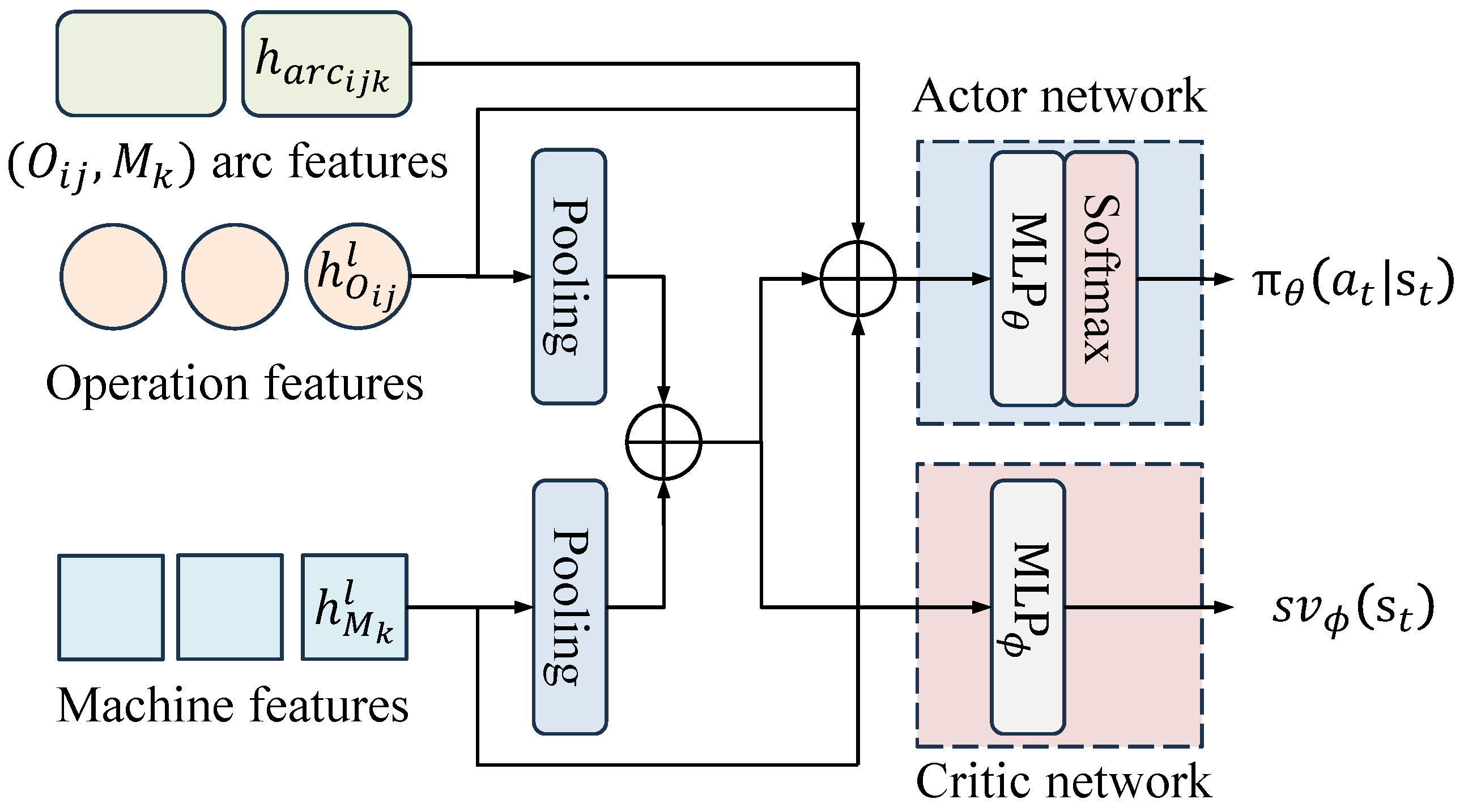
3.5. Decision-Making

We adopt an actor–critic framework parameterized by $\theta$ and $\varphi$ for decision-making, as shown in Figure 5. The actor network aims to generate a policy function ${\pi }_{\theta }\left(a_t\right|s_t)$ for actions. More specifically, for each $a_t$ in ${\mathcal{A}}_t$, say $a_t=(O_{ij},M_k)$, the extracted features of $O_{ij}$ and $M_k$, the global features, and the operation–machine arc features are concatenated into a single vector and fed into the actor network, which outputs the score by

$$sc\left(a_t|s_t\right)={\mathrm{MLP}}_{`}\left[h_{O_{ij}}^{\left(l\right)}\parallel h_{M_k}^{\left(l\right)}\parallel h_{g_t}^{\left(l\right)}\parallel h_{ar{c}_{ijk}}\right].$$

(21)

Then, the probability of selecting $a_t$ is

$${\pi }_{\theta }\left(a_t|s_t\right)=\mathrm{Softmax}\left(sc\left(a_t|s_t\right)\right).$$

(22)

The critic network is used to estimate the state value function. This estimation serves as a baseline to stabilize and improve the efficiency of the training process by reducing variance in the policy gradient. The state value function is estimated by

$$sv\left(s_t\right)={\mathrm{MLP}}_{\varphi }\left(h_{g_t}^{\left(l\right)}\right).$$

(23)

The loss function of [32] is used, which consists of three parts: the policy loss computed by Generalized Advantage Estimation (GAE), the value loss, and the entropy loss used to encourage exploration:

$${\mathcal{L}}_{total}={ϵ}_1{\mathcal{L}}_{policy}+{ϵ}_2{\mathcal{L}}_{value}+{ϵ}_3{\mathcal{L}}_{entropy}.$$

(24)

3.6. Training Process

The actor–critic framework was trained using the Proximal Policy Optimization (PPO) algorithm. The pseudocode is given in Algorithm 1. To improve training stability, we used a reference action network ${\theta }_{old}$ with the same structure as the actor network with lagged parameters. Also, clipping was used to limit the update magnitude of the policy.

We began by initializing the model parameters $\{\omega ,\theta ,\varphi \}$ and sampling $\mathcal{B}$ training instances along with $\mathcal{V}$ testing instances from the simulation environment. The model was then trained over ${\mathcal{N}}_{it}$ iterations, with each iteration starting by setting ${\theta }_{\mathrm{old}}=\theta$. For each instance, a simulation is performed in which the agent interacts with the environment. At each decision point t, an action is sampled from ${\pi }_{{\theta }_{\mathrm{old}}}$ based on the current state $s_t$, and the resulting state transition data is stored in the memory buffer $\mathcal{D}$. The model parameters are updated K times using the collected data. Additionally, the training instances are resampled every ${\mathcal{N}}_{re}$ iterations, and the policy is evaluated on the testing instances. Finally, the memory buffer is cleared at the end of each iteration. We name the proposed approach Multi-Head GAT-based PPO for FJSP-JPC (MGPPO).

Algorithm 1 Multi-Head GAT-based PPO for FJSP-JPC

Input:  Mulit-Head GAT, actor network, and critic network with trainable parameters $\omega$, $\theta$, and $\varphi$; reference behavior actor network ${\theta }_{old}$, Memory $\mathcal{D}$   1: Sample a batch of $\mathcal{V}$ testing instances;   2: Sample a batch of $\mathcal{B}$ training instances;   3: for $iter=1,2,\dots ,{\mathcal{N}}_{it}$ do   4:    ${\theta }_{old}\leftarrow \theta$;   5:    for $b=1,2,\dots ,\mathcal{B}$ do   6:      Initialize state $s_t$ based on instance b;   7:      while $s_t$ is not terminal do   8:         Sample action $a_t\sim {\pi }_{{\theta }_{old}}(·\mid s_t)$;   9:         Receive reward $r_t$ and next state $s_{t+1}$; 10:         Collect the transition ($s_t,a_t,r_t,s_{t+1}$) in $\mathcal{D}$; 11:         Update state $s_t\leftarrow s_{t+1}$; 12:      end while 13:      Compute the generalized advantage estimates $\widehat{A_t}$ for each step using collected transitions; 14:    end for 15:    for $k=1,2,\dots ,K$ do 16:      Compute the total loss function $\mathcal{L}$ with the data in $\mathcal{D}$; 17:      Update the parameters $\theta$, $\omega$, and $\varphi$; 18:    end for 19:    if $iter\%{\mathcal{N}}_{val}=0$ then 20:      Test ${\pi }_{\theta }$ on $\mathcal{V}$ testing instances; 21:    end if 22:    if $iter\%{\mathcal{N}}_{re}=0$ then 23:      Resample a batch of $\mathcal{B}$ training instances; 24:    end if 25:    Empty $\mathcal{D}$; 26: end for

4. Numerical Results

In this section, we first describe the experimental setup. Then, we explore the impact of several mechanisms on the scheduling performance of MGPPO. Finally, we validate the performance of MGPPO by comparing it to some benchmarks.

4.1. Experimental Setup

Test instances. Since there is no established benchmark for the FJSP-JPC, we generated test instances based on the real-world case of a hybrid bicycle assembly job shop presented in [26]. In our formulation, the jobs making up a product are referred to as a job group, which is generated as follows:

1.

Each job group contains 12 operations distributed across six jobs. The number of operations per job is sampled without replacement from the set $1,1,2,2,3,3$.

2.

There are three manufacturing stages, as illustrated in Figure 1. Jobs $J_1,J_2,J_5$ belong to the first stage and have no predecessors. Job $J_3$ is in the second stage, with both predecessor and successor jobs. Job $J_6$ belongs to the third stage, i.e., the final assembly stage, which starts only after all other jobs have been completed.

3.

Following Zhu and Zhou [26], the processing time for each operation is randomly sampled from a uniform distribution $U(100,200)$.

4.

All operations in the final assembly stage must be assigned to a designated machine. For all other operations, two available machines are randomly selected (without repetition) from the remaining machine pool.

The smallest instance includes two job groups, each consisting of six jobs and 12 operations (as illustrated in Figure 1), and involves five machines, denoted as 2 × 12 × 5. Additionally, we consider two larger instance sizes: 3 × 12 × 5 and 4 × 12 × 5. For each size, 1000 instances are randomly generated.

Configurations. We set the training parameters as follows: training iterations ${\mathcal{N}}_{it}=1000$, instances batches $\mathcal{V}=100,\mathcal{B}=20$. The model parameters are updated $K=4$ times per iteration. The training instances are updated every ${\mathcal{N}}_{re}=20$ iterations, and the policy is tested every ${\mathcal{N}}_{val}=10$ iterations. The multi-head GAT module has $l=2$ embedding layers. There are four attention heads in both the operation attention and machine attention blocks per embedding layer. The input dimensions of each head are $d_{o-in}^1=10,d_{m-in}^1=8$ for the first layer and $d_{o-in}^2=d_{m-in}^2=128$ for the second layer. The output dimensions are $d_{o-out}^1=d_{m-out}^1=32$ for the first layer and $d_{o-out}^2=d_{m-out}^2=8$ for the second layer.

In the PPO module, there are two hidden layers with dimension $d_h=64$ and activation function tanh in both the actor and critic networks. In the loss function (24), the coefficients are ${ϵ}_1=1$, ${ϵ}_2=0.5$, ${ϵ}_3=0.01$; the clipping parameter is ${ϵ}_{clip}=0.2$. The learning rate is $lr=3\times {10}^{-4}$, and the minibatch size is 1024.

Performance Metric. We use the results obtained by solving the MILP model with an off-the-shelf solver, Gurobi, as the benchmark. With a time limit of 1800 s, Gurobi can achieve an optimal solution for 2 × 12 × 5 instances and a near-optimal one for 3 × 12 × 5 instances. Given an algorithm, we evaluate its performance by the average relative gap between the makespan obtained by the algorithm $C_{max}$ and the benchmark $C_{max}^{\ast }$:

$${\mathrm{Gap}}^{\ast }=\left({\displaystyle \frac{C_{max}}{C_{max}^{\ast }}}-1\right)\times 100\%.$$

(25)

4.2. Effect of Proposed Mechanisms

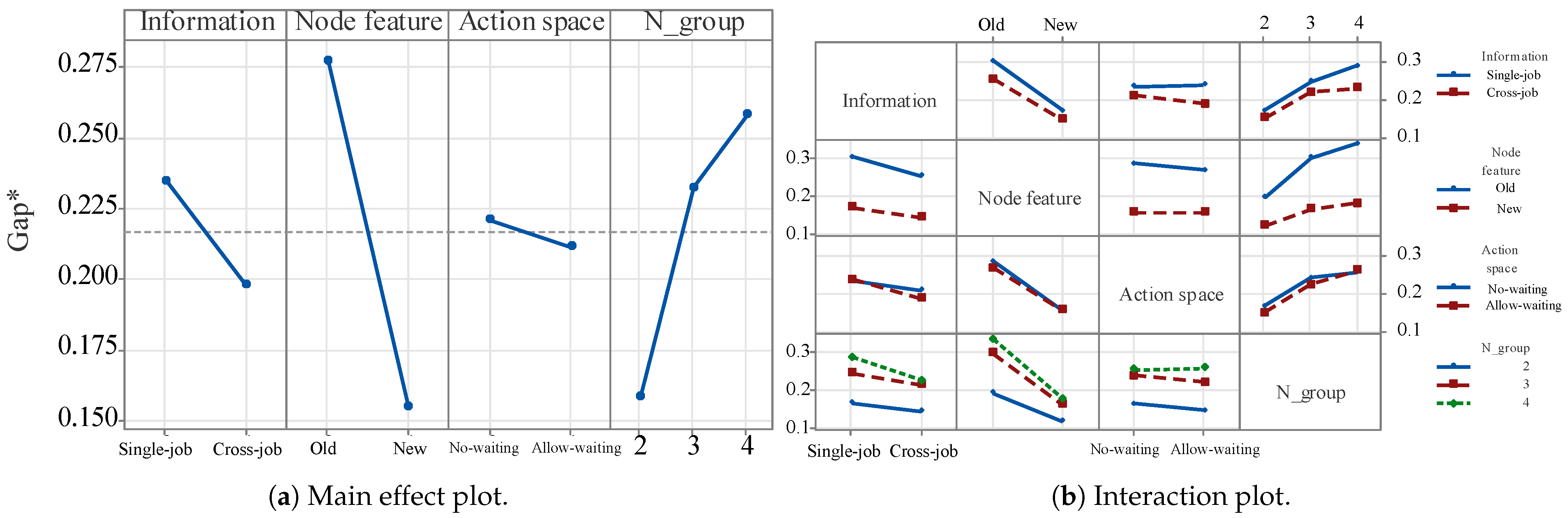
We performed a full factorial design of experiments to investigate the impacts of several proposed mechanisms on the performance of MGPPO. The factors and levels are as follows:

• Information: Single-job, Cross-job;
• Node feature: Old, New;
• Action space: No waiting, Allow waiting;
• N_group: 2,3,4.

The factor “Information” indicates whether the information diffusion is allowed to cross different jobs (cross-job) or restricted to a single job (single-job). The factor “Node feature” indicates whether the node uses features given by [23] (old) or newly designed features (new). The factor “Action space” indicates whether operations are allowed to wait before an idle machine (allow waiting) or not (no waiting). The factor “N_group” indicates the instance size. Each experiment was run for 50 replications. In each replication, the model was first trained and then tested on 1000 instances of the specified size. The gap defined in (25) was used as the response.

The main effect plot is shown in Figure 6a. As shown, all the three modifications led to obvious improvements on the performance. Among them, introducing new node features is the most significant, followed by allowing cross-job information diffusion and allowing operation waiting. From Figure 6b, we observe that allowing operation waiting is more beneficial for small- and medium-sized instances (i.e., 2 × 12 × 5 and 3 × 12 × 5), while its impact is negligible for 4 × 12 × 5. Indeed, allowing operation waiting expands the solution space to include promising solutions; however, as the instance size increases, this advantage is offset by the search inefficiency.

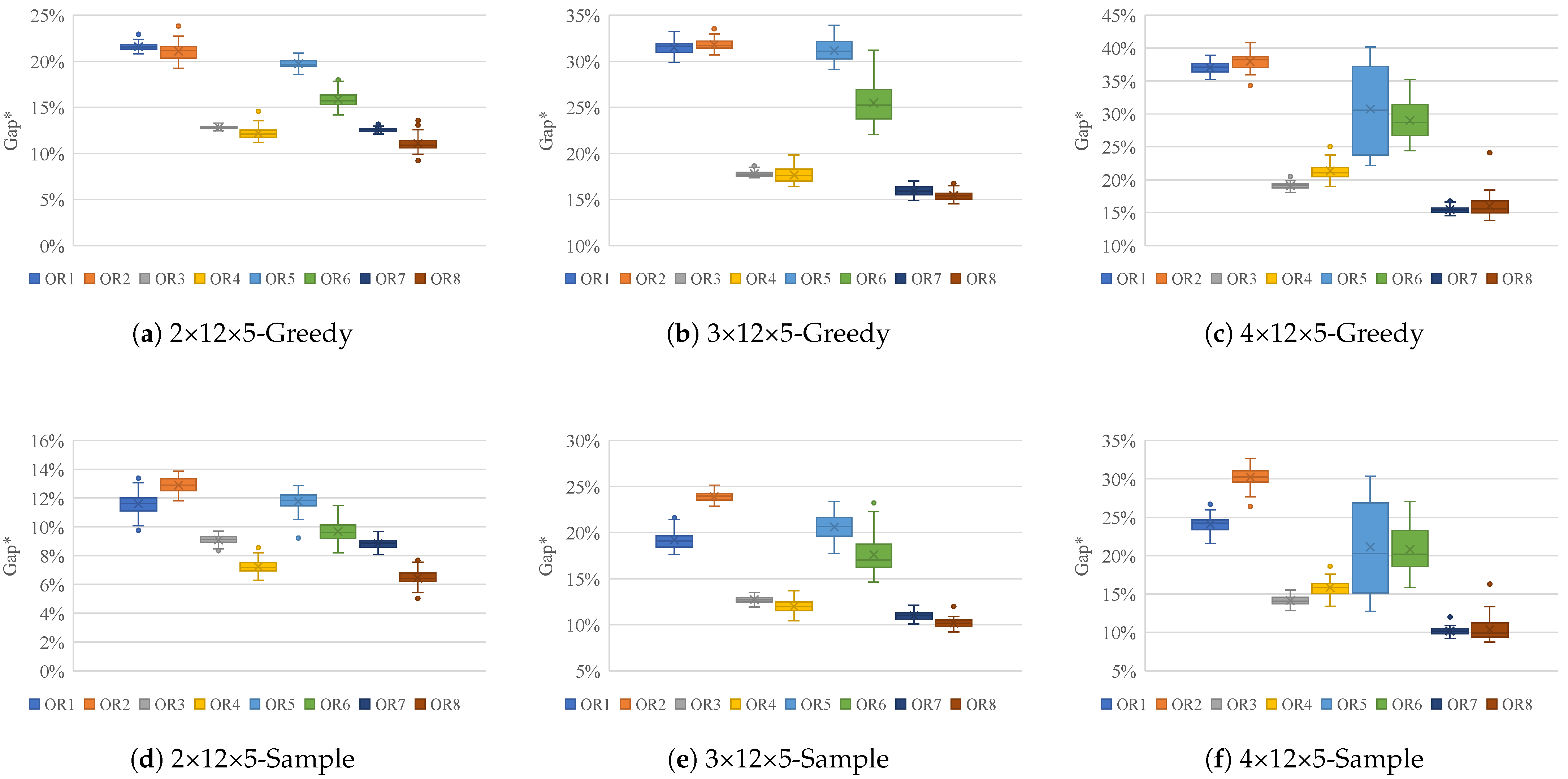
Figure 7 presents boxplots of the average relative gap for MGPPO. The labels OR1–OR8 correspond to the factor combinations listed in

Table 3. Notations for factor combinations.

Exp. ID	Information	Node Feature	Action Space
OR1	Single-job	Old	No waiting
OR2	Single-job	Old	Allow waiting
OR3	Single-job	New	No waiting
OR4	Single-job	New	Allow waiting
OR5	Cross-job	Old	No waiting
OR6	Cross-job	Old	Allow waiting
OR7	Cross-job	New	No waiting
OR8	Cross-job	New	Allow waiting

, with each boxplot summarizing results from 1000 instances. Subfigures (a)–(c) in Figure 7 illustrate the results under the greedy strategy, while (d)–(f) show the results under the sampling strategy. OR1 serves as the baseline configuration without any modifications to the mechanisms, whereas OR8 represents the complete configuration proposed in this paper. As shown, OR8—which incorporates all proposed components—consistently outperforms the other configurations across nearly all problem sizes and both strategies.

4.3. Comparisons with Benchmark Algorithms

We compare MGPPO to four classic priority dispatching rules (PDRs) including First In First Out (FIFO), Most Operations Remaining (MOR), Shortest Processing Time (SPT), and Most Work Remaining (MWKR). These PDRs are combined with machine selection rules to address FJSP-JPC. The implementation details of these rules are provided as follows:

1.

First In First Out (FIFO): Select the candidate operation that is ready at the earliest time and assign it to the first available eligible machine.

2.

Most Operations Remaining (MOR): Select the candidate operation that has the highest number of remaining successor operations (cross-job), and assign it to a random machine that is immediately available.

3.

Shortest Processing Time (SPT): Select the $\left(O_{ij},M_k\right)$ combination with the shortest processing time.

4.

Most Work Remaining (MWKR): Select the candidate operation with the highest average remaining processing time of the remaining successor operations (cross-job), along with a random machine that is immediately available to process the operation.

We also adopted a state-of-the-art DRL algorithm named DANIEL [23] as a benchmark, which was proposed for FJSP. We used the same training and validation parameters as in the original paper. Additionally, we compared the proposed method with a genetic algorithm introduced in [9] with an encoding scheme tailored for FJSP-JPC. The genetic algorithm parameters were configured as follows: maximum iterations 100, population size 400, crossover rate 0.8, and mutation rate 0.1.

Table 4. Performance of different algorithms on instances of size (Number of job groups × Number of operations per group × Number of machines).

Size				Greedy		Sampling		PDRs
		Gurobi 1	GA 2	MGPPO	DANIEL	MGPPO	DANIEL	FIFO	MOR	SPT	MWKR
2 × 12 × 5	${\mathrm{C}}_{\max }$ (s)	1193.16 (100%)	1207.84 (48.3%)	1323.23	1445.10	1269.43	1327.28	1471.01	1597.04	1943.43	1593.45
	Time (s)	0.891	51.801	0.043	0.041	0.857	0.822	0.095	0.099	0.089	0.096
	Gap*	-	1.23%	11.05%	21.59%	6.44%	11.60%	23.74%	34.61%	64.48%	34.24%
3 × 12 × 5	${\mathrm{C}}_{\max }$ (s)	1492.24 (92.5%)	1537.31 (12.5%)	1712.46	1955.90	1633.42	1773.81	1993.91	2167.73	2727.02	2166.79
	Time (s)	161.346	127.597	0.151	0.145	3.019	3.008	0.287	0.291	0.290	0.266
	Gap*	-	3.02%	14.74%	31.49%	9.40%	19.18%	33.98%	45.87%	84.04%	45.82%
4 × 12 × 5	${\mathrm{C}}_{\max }$ (s)	1816.46 (47.9%)	1872.23 (13.5%)	2109.14	2485.37	2007.18	2251.23	2562.07	2754.27	3447.57	2747.28
	Time (s)	1047.276	229.356	0.356	0.352	7.112	7.046	0.580	0.542	0.416	0.427
	Gap*	-	3.07%	15.98%	37.06%	10.36%	24.11%	41.23%	52.02%	90.57%	51.66%

¹ (.%): percentage of instances solved optimally within 1800 s. ² (.%): percentage of instances solved equally or better than Gurobi within 1800 s.

presents the average makespan, Gap*, and computation time of these algorithms on 1000 different instances of specific sizes. For DRL methods, we employed two evaluation methods: greedy and sampling [22]. The former generates a schedule based on the maximum action score, while the latter uses action sampling with (22) to solve an instance 20 times and selects the best one as its result. This allows for utilizing more computational resources to improve the solution quality. Results of the DRL methods are averaged from 50 replications.

Gurobi and GA clearly deliver superior performance; however, their computational times are very long, especially for large instances. In contrast, although PDRs require shorter computational times, they exhibit poorer performance. DANIEL offers better performance than PDRs while maintaining a short runtime. The proposed algorithm outperforms both DANIEL and PDRs across all instances, achieving runtimes comparable to DANIEL. Furthermore, when employing the sampling strategy, the performance of MGPPO is significantly enhanced even with only 20 samples.

5. Discussion

The proposed DRL algorithm has proven to be a promising approach to FJSP-JPC. Its advantages stem from the tailored node features, the information diffusion mechanism, and the well-designed action space of MGPPO. The proposed method has no special requirements for the scale and structure in the instances. This means that even if changes occur in jobs and machines in the environment during the scheduling process, they will not affect the feasibility of the method. Theoretically, our method is not only applicable to FJSP-JPC, but also to the classical FJSP (where the predecessor job of each job is regarded as an empty set). In the future, experiments can be designed to validate the generality of this method.

Unlike methods such as Gurobi and GA, which generate the entire schedule at once, this approach makes incremental decisions based on the real-time status of the shop floor. As a result, even if the manufacturing process is disrupted by disturbances, the algorithm can respond flexibly. Moreover, the negligible decision time for each step makes the proposed algorithm highly applicable in dynamic environments, such as the modular flexible automotive assembly workshop, which is highly relevant to FJSP-JPC. Companies of this kind are frequently confronted with abrupt disruptions such as order changes or machine failures, and our method can effectively enhance production efficiency in such scenarios.

6. Conclusions

In this paper, we propose a deep reinforcement learning approach, named MGPPO, for solving FJSP-JPC. It employs a heterogeneous disjunctive graph to represent the shop floor status and utilizes a multi-head graph attention network to efficiently extract problem features. These features are then fed into an actor–critic framework, where the actor generates operation sequencing and machine assignment decisions simultaneously, while the critic evaluates the policy. The entire model is trained using the PPO algorithm.

Through experiments, we show that the proposed approach consistently outperforms traditional dispatching rules and a state-of-the-art DRL method. Key factors contributing to its performance include improved node features, cross-job information diffusion, and an enhanced action space.

In addition, our research for FJSP-JPC still has certain limitations, and future work can be carried out in the following aspects: first, the experiments in this paper consider no disturbance factors. In actual production environments, multi-source disturbances such as machine failures, order changes, and raw material shortages often intertwine, further increasing the solving difficulty of scheduling problems. Future work will focus on extending this approach to dynamic manufacturing environments with real-time disruptions and further enhancing its generalizability across various production scheduling problems.

Second, this paper only considers makespan as the optimization objective, without taking into account other practical production objectives such as equipment energy consumption, load balancing, and total tardiness. Future work can be expanded to multi-objective optimization by incorporating the diversified needs of intelligent manufacturing, designing weighted reward functions or Pareto front search mechanisms to balance indicators like production efficiency and sustainability.

Third, in the common scenarios of FJSP-JPC investigated in this paper (e.g., automotive assembly), companies typically face constraints on transportation resources and the collaborative scheduling of transportation and processing resources. Operations not only require a selection of processing machines but also match with available transportation equipment, as transportation delays may become production bottlenecks in actual manufacturing. Future work can develop problem models considering transportation resource constraints for further investigation.