Article

A Machine Learning Approach for Mechanical Component Design Based on Topology Optimization Considering the Restrictions of Additive Manufacturing

by
Abid Ullah
1,2,*,†,
Karim Asami
1,*,†,
Lukas Holtz
1,3,
Tim Röver
1,
Kashif Azher
4,
Katharina Bartsch
1,5 and
Claus Emmelmann
1
1
Institute of Laser and Systems Technology, Hamburg University of Technology, 21079 Hamburg, Germany
2
Centre for Additive Manufacturing, School of Engineering, RMIT University, Melbourne, VIC 3000, Australia
3
Teccon Consulting & Engineering GmbH, H2ERD Department, Karnapp 25, 21079 Hamburg, Germany
4
Department of Mechanical Engineering, King Fahd University of Petroleum and Minerals, Dhahran 31261, Saudi Arabia
5
Fraunhofer Institute for Additive Production Technology IAPT, Am Schleusengraben 14, 21029 Hamburg, Germany
*
Authors to whom correspondence should be addressed.
These authors contributed equally to this work.
J. Manuf. Mater. Process. 2024, 8(5), 220; https://doi.org/10.3390/jmmp8050220
Submission received: 23 July 2024 / Revised: 13 September 2024 / Accepted: 26 September 2024 / Published: 1 October 2024
(This article belongs to the Special Issue Design, Processes and Materials for Additive Manufacturing)

Abstract

:
Additive manufacturing (AM) and topology optimization (TO) emerge as vital processes in modern industries, with broad adoption driven by reduced expenses and the desire for lightweight and complex designs. However, iterative topology optimization can be inefficient and time-consuming for individual products with a large set of parameters. To address this shortcoming, machine learning (ML), primarily neural networks, is considered a viable tool to enhance topology optimization and streamline AM processes. In this work, a machine learning (ML) model that generates a parameterized optimized topology is presented, capable of eliminating the conventional iterative steps of TO, which shortens the development cycle and decreases overall development costs. The ML algorithm used, a conditional generative adversarial network (cGAN) known as Pix2Pix-GAN, is adopted to train using a variety of training data pairs consisting of color-coded images and is applied to an example of cantilever optimization, significantly enhancing model accuracy and operational efficiency. The analysis of training data numbers in relation to the model’s accuracy shows that as data volume increases, the accuracy of the model improves. Various ML models are developed and validated in this study; however, some artefacts are still present in the generated designs. Structures that are free from these artefacts achieve 91% reliability successfully. On the other hand, the images generated with artefacts may still serve as suitable design templates with minimal adjustments. Furthermore, this research also assesses compliance with two manufacturing constraints: the limitations on build space and passive elements (voids). Incorporating manufacturing constraints into model design ensures that the generated designs are not only optimized for performance but also feasible for production. By adhering to these constraints, the models can deliver superior performance in future use while maintaining practicality in real-world applications.

1. Introduction

Additive manufacturing (AM) is becoming increasingly important in today’s manufacturing landscape. From the production of spare parts to lightweight construction, various AM processes enable the direct production of complex geometries [1,2,3]. The component is built up in a layer-by-layer fashion in these manufacturing processes and offers a high degree of design freedom. With the continuous advancements in AM processes and the resulting cost reductions, it is now possible to explore new domains and produce functional components. The numerous advantages of AM include producing lightweight products, complex geometries with improved performance, and individualization [4,5]. Despite advancements in manufacturing technology, the design process for AM still requires streamlining. Improving the performance and durability of manufactured components through optimal design and weight reduction is most desirable since it also directly contributes to the efficiency of energy and raw material consumption [6,7].
Topology optimization (TO) is an interesting area of structural optimization that is particularly indispensable for AM designs. TO has advanced significantly in recent years, particularly due to educational codes published in the literature [8,9,10,11,12]. Because of the versatility of TO, organic designs with firmly interconnected features are frequently seen. Although optimal designs are achievable when compared to other structural optimization approaches, TO was previously purely theoretical due to limitations in manufacturing procedures to actualize such designs [13]. However, due to the continual development of the AM processes, there have been significant efforts in the past decade to incorporate TO into the design workflow of various products [14,15,16]. Nevertheless, the varied and complex AM processes create new guidelines and limitations, which must be carefully considered while creating TO algorithms for AM. TO using the finite element method is well-recognized for producing highly precise structures [17,18]. However, this approach can be computationally costly. Based on the geometrical dimensions and available computer resources, the computing time ranges from minutes to days [19,20]. In recent times, the manufacturing of products with specialized features such as complex, individualized, and topology-optimized lightweight items is now directly achievable thanks to modern AM technologies [21,22,23]. This advancement opens up significant optimization potential, which can be exploited with the help of machine learning (ML). ML has gained popularity in various research fields such as natural language processing [24], finance [25], image processing [26], robotics [27], and mechanics [28] due to its capacity to identify complicated patterns in vast datasets. Thanks to increased computational power and easy access to vast amounts of data, this technology has greatly evolved in recent years [29,30,31]. Consequently, ML plays a crucial role in optimizing the parameters needed for AM design and production.
Over the past decade, numerous studies have focused on the design or redesign of components for sectors such as the automotive, aerospace, and medical industries. These studies also examined process-influenced geometrical constraints and the formation of cavities during AM. Applying ML algorithms to create topology-optimized structures is a stimulating and emerging subject of study [12]. For instance, Shin et al. [20] provide a comprehensive discussion of how ML technologies, such as deep learning, are increasingly utilized to optimize structural designs by predicting optimal material distributions and decreasing computational overhead. These methods use neural networks to optimize the TO process, leading to faster and more accurate results. Similarly, researchers introduced a real-time TO strategy utilizing ML and demonstrated its application in developing optimal designs for AM [32,33,34,35]. Wu et al. [36] established an optimization framework for additively manufactured lattice structures that incorporates a derivative-aware neural network to predict material properties and optimize unit-cell geometries for uniform strain patterns, which was validated through experimental tests and digital image correlation analysis.
Algorithms and neural networks enable the independent recognition of patterns and regularities in datasets, allowing them to solve problems independently [37]. This capability is particularly relevant to the manufacturing of bespoke components. Customizing a product with numerous parameters can quickly lead to millions of variants, making iterative TO for each variant costly and time-intensive. ML can influence TO using different methods [38,39,40]. Some deal with the improvement of algorithms in TO [38,40], and others with the complete substitution of TO by artificial neural networks [39].
This work aims to develop an ML model that generates parameterized topology-optimized AM products. Using a parameterized, topology-optimized cantilever as an example, the objective is to demonstrate that an optimized and configured product tailored to customer requirements can be quickly generated using the ML model. Traditional topology optimization approaches are time-consuming and demand constant computer resources for each design iteration. This study fills a gap by showing that, once trained, the ML model can create optimum designs in milliseconds, providing a very efficient solution for repeating or large-scale design tasks. The proposed ML model also offers the capability to provide customers with real-time product proposals that align with their unique specifications. Finally, a selected design can be manufactured through the laser powder bed fusion process or other laser-based AM techniques.

2. Methodology

The design approximation for the TO of a cantilever beam, ML algorithms, a fundamental explanation, the cantilever beam’s used parameters, and the dataset are all explained in this section.

2.1. Design Approximations

The parametric topology 2D cantilever design was generated following seven different dataset models. The models were performed within a constant build space of 100 × 100 elements. The decision to use a square build space was made because most algorithms are designed to work with square matrices. A higher resolution for the design space was avoided to minimize the computational effort required for TO and calculate computing time. Resolution in topology optimization refers to the level of detail or granularity at which the material distribution within a design domain is optimized or improved [41,42]. To balance computational efficiency and the result’s quality, we employed a lower-resolution design space. To be able to program in Python 3.11, the Anaconda distribution (by Anaconda, Inc., Austin, TX, United States) was used. The design configuration was fixed to a floating bearing-fixed bearing combination. Specifically, the floating bearing was positioned in the upper left corner, while the fixed bearing was located in the lower left corner. To balance computational efficiency and optimization quality, the iteration number for the TO was set to 70. Additionally, the average function change in the 70th iteration was constrained to be under 0.02 (at a resolution of 100 × 100 elements), further ensuring the optimization process’s effectiveness. The parameters used for the TO remained constant throughout all steps. A step in this study refers to the distinct boundary conditions or some geometric features that occur within the iterative process. As the number of dependencies and the complexity of those dependencies, especially in boundary conditions, increase with each step, the numerical solution becomes inherently more challenging to attain. Consequently, this process increases the complexity of obtaining the numerical solution. In-depth knowledge of these procedures is essential for analyzing how the heightened complexity impacts the overall performance and accuracy of the algorithm compared to traditional TO methods. The specifications primarily revolve around the installation area, as this cantilever is designed with a focus on topology optimization. The type and placement of the clamping mechanism can range from fixed loose mountings to multiple permanent clampings.
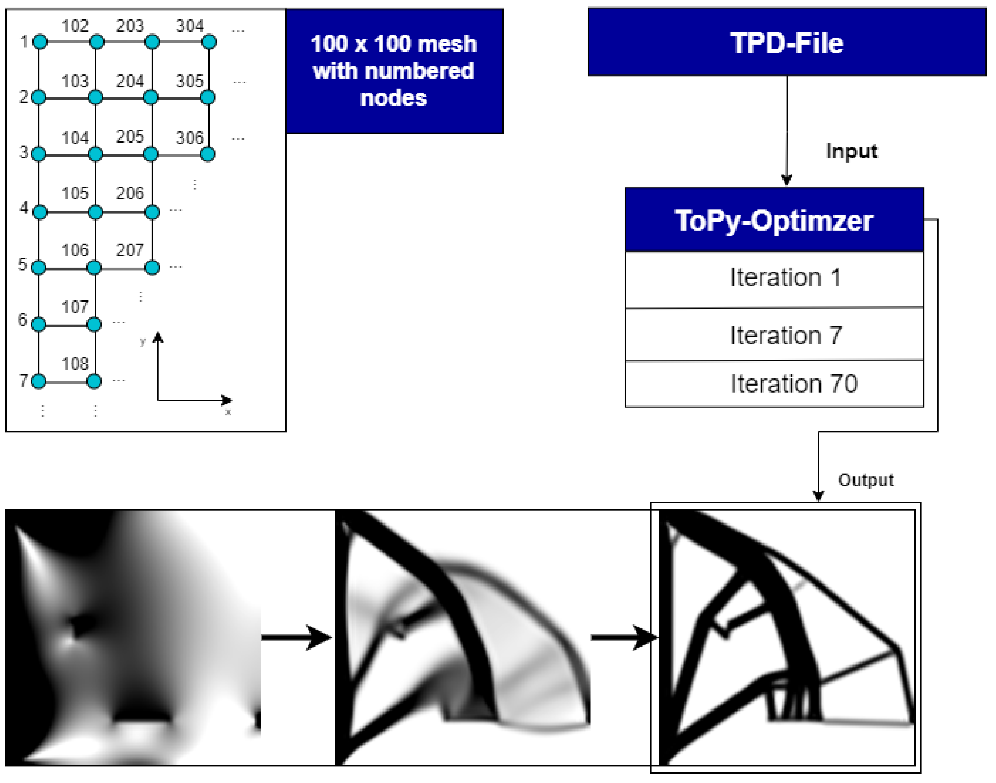
Additionally, the applied forces, including their varying amplitudes and specific points of application, introduce further variables. The nature of the forces involved further defines these parameters; both distributed loads and point loads are potential factors that need to be taken into account. All steps performed during design optimization, along with the program, are shown in Figure 1. All variable parameters, encompassing factors, such as restraint type, restraint positions, construction area dimensions (height and breadth), force type and count, applied force locations, applied force magnitudes, and passive components, are encompassed within the foundational framework. Passive components refer to elements that are intentionally left unfilled. The generation of picture data within this foundational framework, where parameters are structured in a matrix, will be implemented using the ToPy library. The outcome will be translated into an image representation. Simultaneously, the parameter details will be stored in a ToPy Problem Definition (TPD) file, which can be directly fed into the optimizer for further processing. To provide a data pair to the algorithm, the optimizer generates an image file, which is then paired with the corresponding parameter image. This methodology involves iteratively constructing a weighted model using diverse training datasets. Subsequently, a separate test dataset is employed to validate this model. During validation, the weighted model is utilized to generate a model’s geometry from images containing parameter data. This process is juxtaposed with topological optimization generated by the optimizer.

2.2. ML Approach

The programming phase involves various essential tasks, such as creating program codes for validation, training data generation, and implementing an artificial neural network (ANN) algorithm. An ANN is a versatile machine learning technique used for both regression and classification tasks, inspired by biological neural networks in the human brain [43,44]. It is applied to complex tasks such as classification, regression, and pattern recognition by assigning classes to data points based on the characteristics of their nearest k neighbors. In essence, the algorithm looks at the k closest data points that have already been assigned classes and takes a majority vote among them to determine the final classification for the new data point. One of the notable advantages of the straightforward ANN algorithm is its minimal input requirements. It only necessitates the specification of two key parameters: the value of k, which determines the number of neighbors considered, and a distance measure that quantifies the proximity between data points [45]. This simplicity makes the algorithm relatively easy to implement and apply. An ANN emulates the intricate neural mechanisms of the human brain. Like brain networks, ANNs consist of interconnected neurons. These neurons compute inputs to generate outputs, with their interconnections forming a network. Mathematical formulas within neurons act as weights, adapting computations based on input data. ANNs usually have three components: input, hidden, and output layers. They are versatile and used in supervised learning for predictions/classifications and unsupervised learning for pattern exploration.
An instance of this concept is the generation of synthetic image data through a generative adversarial network (GAN) system. Comprising the GAN are two artificial neural networks: the discriminator and the generator. The generator employs random noise as input to craft a fabricated (false) image, for instance, one depicting topology optimization. Subsequently, this image is presented to the discriminator. Furthermore, the discriminator is exposed to images from the training dataset. It then evaluates the authenticity of the image it encounters on a scale from zero to one, categorizing it as genuine (closer to zero) or counterfeit (closer to one). Through training, both artificial networks continually enhance their capabilities. A neural network serves as a suitable tool for discerning intricate correlations and has the potential to supplant the iterative stages of TO entirely. Moreover, it is amenable to parameterizable topology optimization, wherein input parameters such as force application sites and amplitudes can be modified. A specific variant of the conditional generative adversarial network (cGAN) proves effective for complex input matrices. Deep learning, a machine learning derivative, uses the cGAN, which allows machines to learn independently by generating and discriminating images more precisely. cGAN was introduced by Mehdi Mirza and Simon Osindero in 2014 [46]. The generator and discriminator can receive more precise class labels to guide their data generation with a conditional GAN. These details help the generator and discriminator specify their data and obtain results faster. Labels help the generator produce more specific data. Depending on the label, it will produce images of pants, jackets, or socks. Labels help the discriminator’s network distinguish real images from generator-provided fakes, improving efficiency [47].
A condition is introduced to the cGAN, which is then incorporated into both the generator and discriminator components. This condition could manifest as a matrix or a label. Consequently, in scenarios such as picture-to-image translation, both networks possess knowledge about the specific image category under consideration. This capacity enables the incorporation of supplementary input to the model through the application of the cGAN framework [48,49]. During training, the Pix2Pix algorithm is provided with pairs of images. One image includes the forces and constraints influencing topology optimization, while the other displays the corresponding topology optimization outcome, as depicted in the illustration. This mode of learning falls under supervised learning, given that the algorithm was trained using these paired datasets.
Known parameters are incorporated into the basic framework of training data generation, which automatically varies different parameters to generate diverse datasets. This user-adjustable framework ensures the output of relevant training data tailored to the chosen ML algorithm, leading to accurate results. Once the basic framework is established, the selected ML algorithm is integrated into the programming language environment to create models using the generated training data. Subsequently, the ML model’s output is validated to assess its accuracy, with automated validation through program codes being the preferred method due to the substantial volume of data involved. Accuracy in machine learning assesses a classification model’s performance by measuring the proportion of accurate predictions to total predictions, expressed mathematically as follows [50].
A c c u r a c y = T P + T N T P + F N + T N + F P
where true positives are TP, true negatives are TN, false positives are FP, and false negatives are FN.
The ML algorithm is directly integrated with TO, offering a powerful combination of capabilities. While it is possible to use a TO algorithm from another programming language to achieve automated parametric TO, for this work, we chose an implementation leveraging Python 3.11 due to its familiarity and ease of use. This allowed us to adopt the solid isotropic material with penalization (SIMP) method through the use of ToPy. The SIMP algorithm is a common approach in TO that starts with a uniform material distribution. It uses equilibrium equations and sensitivity analysis to guide the design changes, aiming to improve performance metrics such as compliance. Recent studies have explored combining SIMP with ML techniques, such as neural networks, to enhance TO [51,52,53].
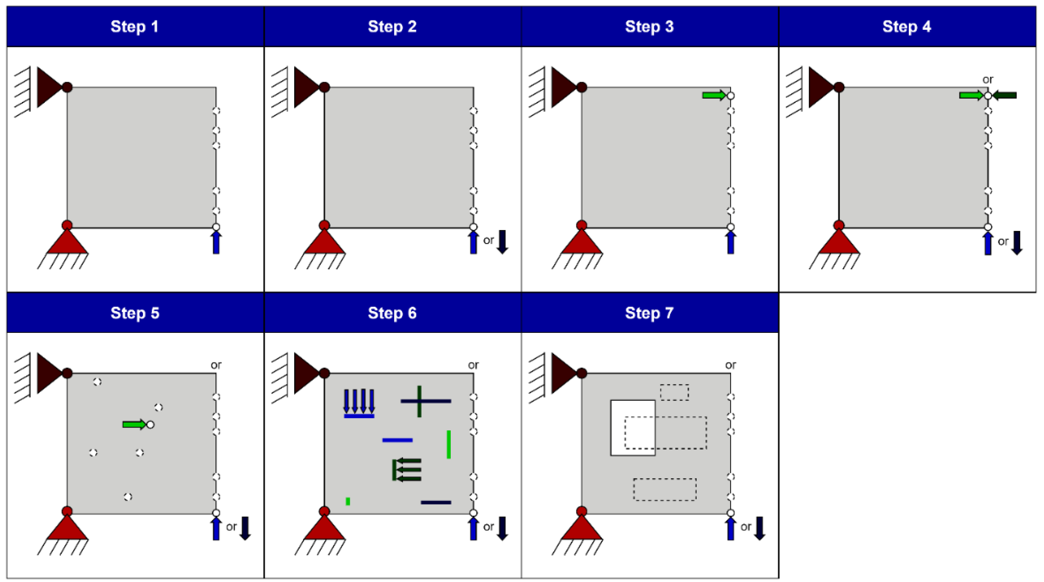
The decision to use ToPy in this study was driven by the goal of reducing the time required for familiarization with multiple programming environments while leveraging the advantages of Python in the context of TO. These parameters were derived from recommended and well-established settings of ToPy. The design space does not have a higher resolution, as this would significantly increase the computational effort required for topology optimization. The clamping was fixed using a combination of a floating bearing and a fixed bearing. Due to the substantial computational effort required for generating training data, not all implemented parameters could be subjected to variation. The parameters subject to variation include location, orientation, amplitudes, and load types. Additionally, passive elements were integrated to explore the behavior under manufacturing constraints. Employing the predefined optimization algorithm parameters, topology optimization using ToPy and the mentioned hardware yielded an average processing time of 90 s. Consequently, generating 10,000 sets of training data demanded 250 h. However, it is worth making clear that the 250 h required to train the ML model is a one-time cost. Once trained, the ML model can create optimum designs in milliseconds, significantly lowering the time required for subsequent design development. This makes the ML technique extremely efficient for repetitive or large-scale design jobs, as opposed to classical topology optimization, which incurs ongoing computing costs. The topology optimization process was limited by processor speed (CPU-bound) and did not fully leverage the capabilities of the 12-core processor (utilization was at 25% for a single topology optimization). This enabled the concurrent execution of four topology optimizations, effectively reducing the computation time required for 10,000 sets of training data to 62.5 h. However, this study introduced variations in certain parameters to investigate the design behavior under different conditions. The variable parameters included the location, orientation, amplitudes, and type of loads. Furthermore, passive elements were also implemented to assess the cantilever’s performance when subject to manufacturing constraints. The specific variable parameters are illustrated in Figure 2 for reference.

2.3. Parameters Utilized

Table 1 and Figure 3 present the sequential process for creating the models. The first column lists the individual steps from steps one to seven. The second column displays the varying parameters, along with the maximum possible variations achievable within those parameters. The last column indicates the number of training data pairs used, representing a fraction of the possible variations. In the initial step, the point load’s location varies along the design space’s right outer edge. This choice is based on the typical loading of a cantilever structure, where the load is applied at the far end opposite from the bearing. Consequently, this step allows for 101 possible variations corresponding to the number of nodes in the Y-direction. Progress in each step is changed and a new combination of varying parameters is introduced. In the final step, variations are applied to the location and orientation of a point load and the inclusion of passive elements. This step explores the effects of manufacturing constraints on component volume, displacement, or manufacturing boundary conditions.
The equations governing the traditional topology optimization process are provided here. The optimization problem can be formulated as (as per pix2pix cGAN):
M i n i m i z e   C u , v = f T u
s u b j e c t   t o
K v u = f
where C is the compliance, u is the displacement vector, v represents the design variables, K is the stiffness matrix, and f is the external force vector.
For our ML model, we employ a conditional generative adversarial network (cGAN), where the objective function for the generator G and the discriminator D can be defined as:
L c G A N ( G , D ) = E x , y [ l o g D ( x , y ) ] + E x , z [ l o g ( 1 D ( x , G ( x , z ) ) ) ]
Additionally, the generator is optimized with an L1 loss to encourage the production of realistic designs:
L L 1 G = E x , y , z [ y G ( x , z ) 1 ]
The total objective function is a weighted sum of these losses:
G * = a r g m i n G m a x D L c G A N ( G , D ) + λ L L 1 ( G )
where λ is a weight parameter balancing the two loss components.
Further fundamental mathematical equations and topology optimization formulas are available in the References [54,55,56,57].

3. Results

3.1. Assessment of ML Design Models

In Table 1, seven different steps or models are presented with varying load types, locations, natures, and datasets. Distinct phases were defined, each possessing unique attributes that broadened the spectrum of potential variations. Numerous potential deviations were selected as training data. However, a substantial increase in training data was unattainable due to hardware constraints, particularly for a higher count of variations. The augmentation of training data was incrementally decided, commencing with a limited dataset and culminating in a maximum threshold of 30% of the total variations at hand.
The term accuracy refers to the deviation between the generated image and the TO image used to explain the models. In the first step, 30 training data pairs were created to train the model using a constant point load in the positive Y-direction along the outer right edge of the build space. The model was trained with these data pairs, and its performance was evaluated across multiple epochs. An epoch in machine learning refers to one complete pass through the entire training dataset, and it influences model performance, with higher numbers generally improving accuracy by providing more learning opportunities. However, too many epochs can lead to overfitting [49,58]. It is determined by averaging the absolute deviations between each data point and the dataset’s mean. A smaller mean deviation indicates that the data are more closely packed around the mean, thus providing a measure of how the data are spread out. During the model evaluation, cross-validation and the scores obtained in each fold are often used and calculated as their mean, minimum, maximum, and standard deviation. At epoch 10, the mean deviation was measured to be 7.2%, which improved to 5.7% at epoch 20. The most significant enhancement was observed in epoch 40, where the mean deviation reached its lowest value of 5.1% compared to the original TO. Concurrently, the minimum deviation started at 3.9% and gradually decreased throughout the 300 epochs, reaching 1.69% at the end. The maximum deviation fluctuated between 12.8% and 10.7% across the epochs. Figure 4 illustrates the consistent improvement of the model as the epochs progressed. The early epochs produced somewhat unstable results, but the generated images became smoother and more accurate with time. This is due to underfitting from the dataset. An entire run-through of all the training data is called an epoch. The constructed model becomes more accurate (theoretically) the more times these are run through. The code generates a model every ten epochs; hence, at an epoch count of fifty, five models, all of which are validated, are produced [59]. The model may not have been exposed to enough variability in the data with fewer epochs, which would have resulted in poor generalization. Consequently, the topology optimization may not work effectively in unknown settings, producing inconsistent or erroneous outcomes. Despite the model’s continuous improvement, some of the early results still exhibited artefacts or significant deviations from the original TO.
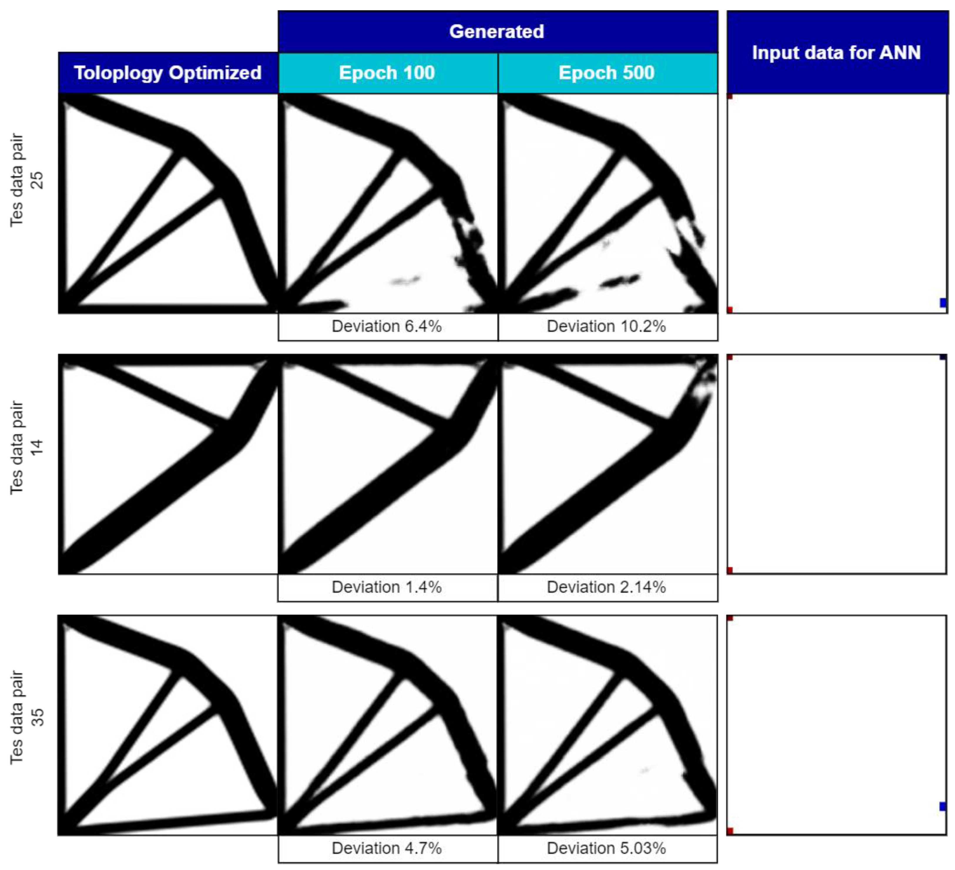
Moving to the second step, with improved data pairs from 30 to 65, significant improvements were evident in the generated images compared to the first model. Both the minimum and mean variations were notably reduced. The second model utilized a slightly higher percentage of the possible 202 variations in the training data, with the absolute number of training data increasing from 30 to 65. However, the complexity of the model did not change significantly. The second model demonstrated improved translation of color-coded images into topology-optimized (TO) structures, resulting in fewer artefacts. Training for more than 100 epochs yields no discernible advantages for the second step and, in some cases, even leads to the emergence of additional artefacts. Although increasing the number of epochs might be beneficial in properly training a machine learning model, using an excessively large number of epochs can result in overfitting, numerical instability, and other problems that lead to topology optimization outcomes that are unstable or fall short of the ideal. A comparison between the generated structures from epoch 100 and epoch 500 is illustrated in Figure 5.
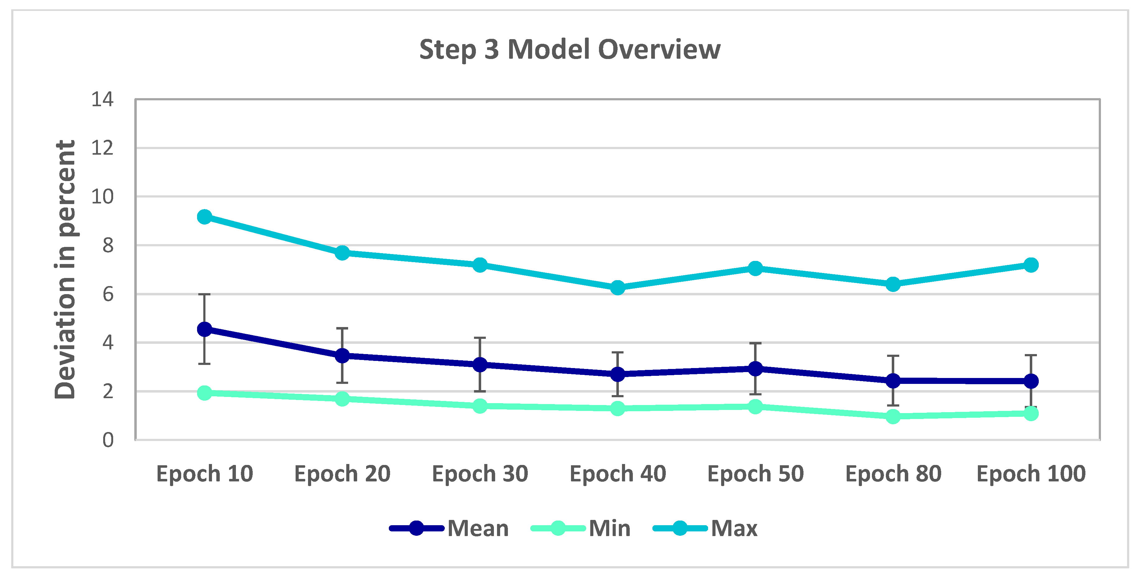
Artefacts and deviations are present in the generated images; therefore, the third step with increased training data has led to a noticeable reduction in artefacts in the generated images. However, some test pairs still exhibit the strongest deviation, with unconnected structural elements, while the other fine structures can be accurately reproduced with a deviation of only 1.42% in epoch 100. Model 3 employed only 6.8% of the possible variations as training data, outperforming Model 2 in terms of mean, maximum, and minimum values. The absolute number of training data has remarkably increased from 65 in Model 2 to 700 in Model 3. Out of the 100 test data samples, nine of them still contain implied or incomplete structures. However, this percentage is slightly lower than in Model 2, despite the increased complexity of introducing a new force component. Moreover, the occurrence of artefacts in the generated images has diminished with the substantial increase in training data. A collection of these generated images is presented in Figure 6. Among them, the generated image corresponding to test data pair 37 exhibits the most significant deviation, displaying disconnected structural elements. Additionally, as evident in test data pair 100, intricate features can be accurately replicated by the ANN with only a 1.42% deviation observed in epoch 100. This suggests that further increasing the training data would likely lead to even fewer remaining artefacts.
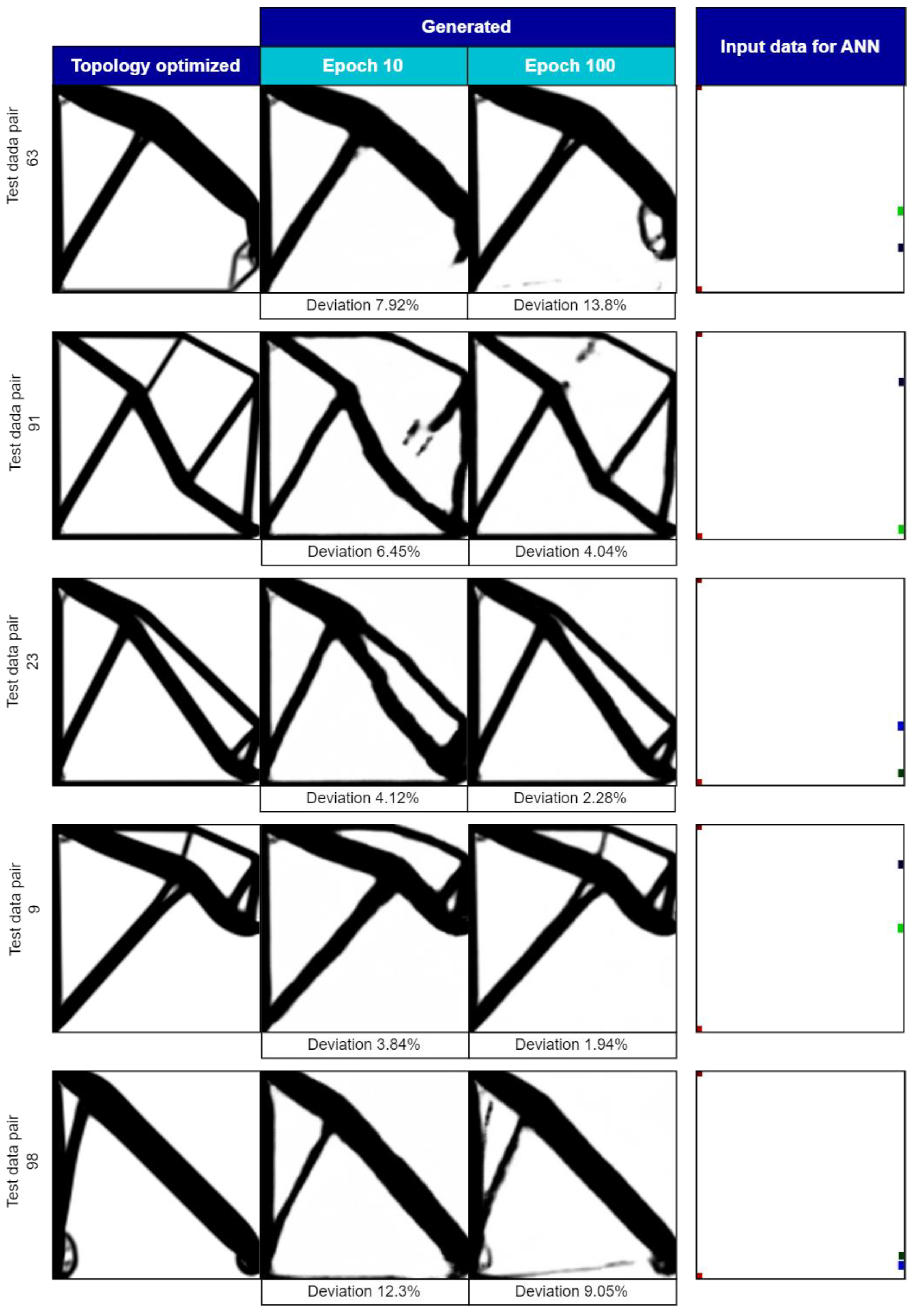
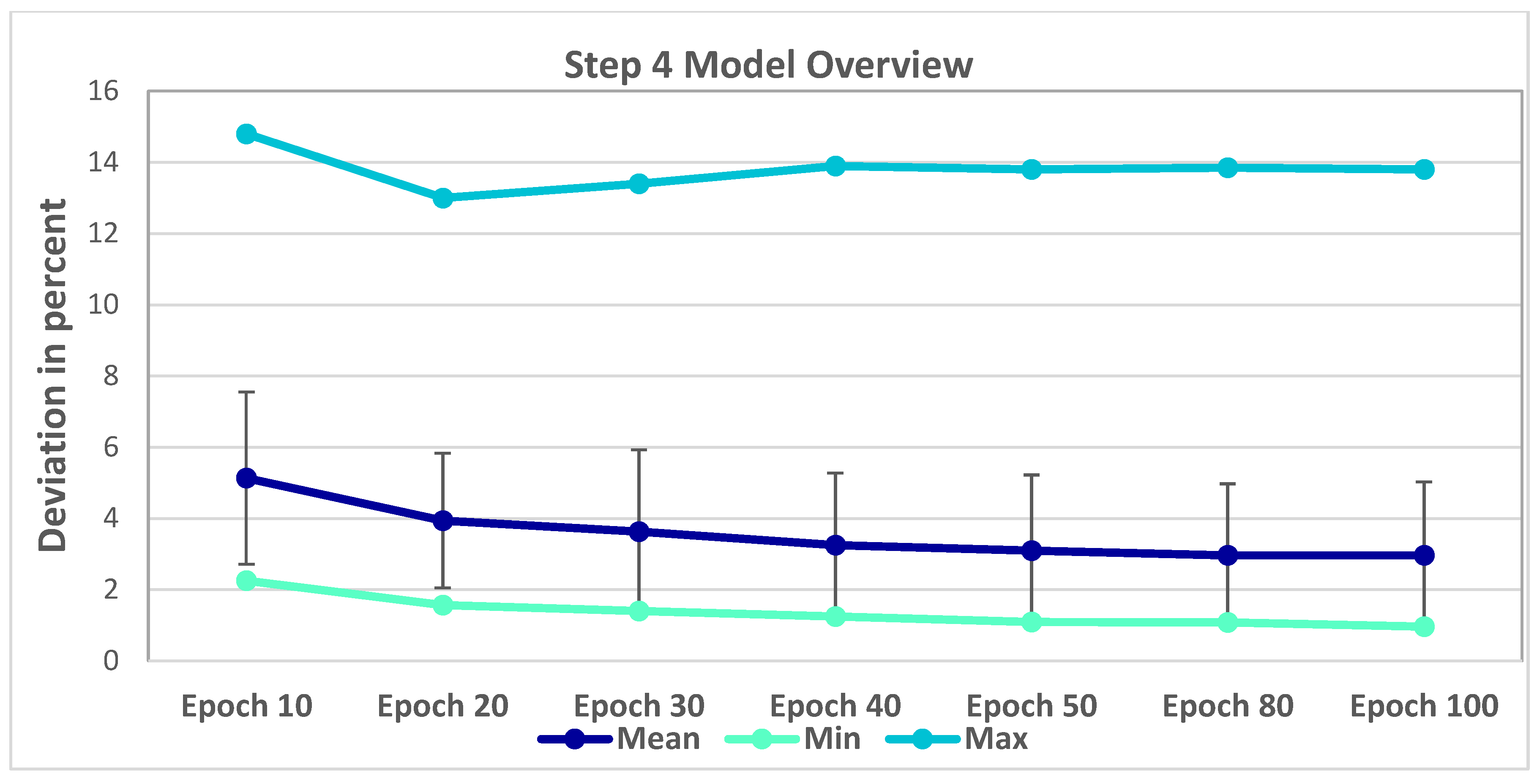
In the fourth step, it becomes evident that the generation of finer structures is only achievable with increasing epoch numbers, where the fine structures become more accurately reproduced as the epochs progress. Model 4 utilized 3.7% of the possible variations as training data, which is only slightly higher than the third model. Despite the relatively small increase in training data percentage, the mean value of the fourth model exhibits only a slight improvement compared to the third model. Similarly to Model 3, nine out of 100 test data samples in Model 4 still show implied or incomplete structures, despite the increased complexity introduced by changing the force directions. Figure 7 illustrates the disparities between epoch 10 and epoch 100. Once again, it becomes evident that finer structures are achievable only through the progression of epoch numbers. This phenomenon is exemplified by the cases of test data pair 9 and test data pair 63. The fourth model comprises 3.7% of all possible variations in its training data, resulting in a slightly augmented mean value compared to the third model. Similar to the third model, nine out of the 100 test data exhibit implied or incomplete structures, despite incorporating increased complexity by altering the force directions. Hence, it is expected that further increasing the training data would lead to a reduction in the remaining artefacts. The models one to four are compared in Figure 8 and Figure 9. Among Models 1, 2, 3, and 4, Model 3 seems to be more accurate regarding lesser deviations. The deviation value also proves the lesser artefacts present in the TO geometry.
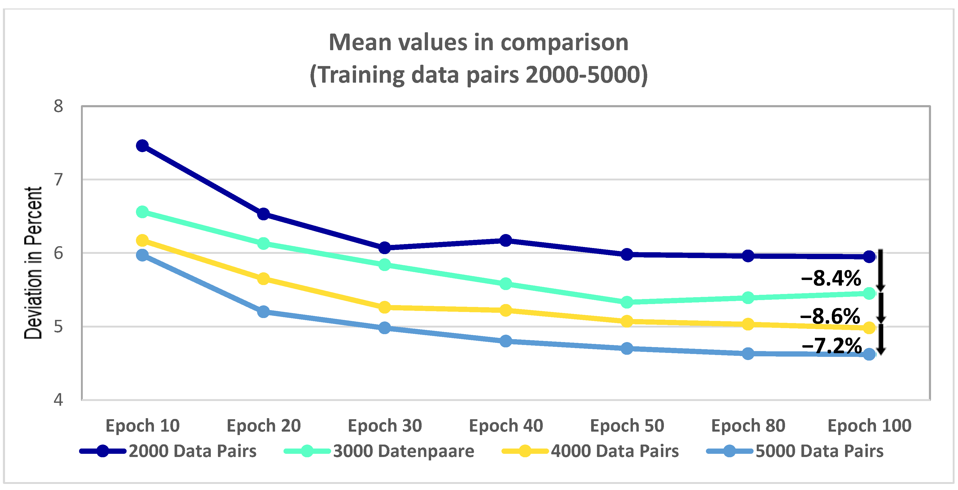
In the fifth step, the training data were systematically varied in increments of thousands, ranging from 2000 to 5000 data pairs. The analysis reveals a consistent and notable improvement in accuracy with the increase in the number of data pairs. For instance, from Figure 10 for 2000 training data pairs, the mean value at epoch 100 reaches 5.95%. In contrast, for the model with 5000 training data pairs, the mean value at the same epoch improves significantly, reaching 4.62%. This represents a substantial 22.4% enhancement compared to the accuracy of the first model. Furthermore, the effect of adding training data notably leads to a reduction in artefacts. For instance, significant difficulties are encountered in the model with 2000 training data pairs in accurately representing fine structures. However, in the model with 5000 training data pairs, all structures are more precisely pronounced and almost entirely connected. Despite the overall improvement in accuracy with the increased training data, the fifth model exhibits a higher number of artefacts compared to the previous models. Out of the 200 test data samples, 32 generated images demonstrate unconnected structures or strong artefacts. Although the generated images in this model may exhibit a certain degree of similarity to the TO results, the presence of unconnected structures significantly affects the overall stiffness of the optimized designs. This indicates that while the model resembles the desired topology, the integrity and performance of the final product are compromised due to these artefacts.
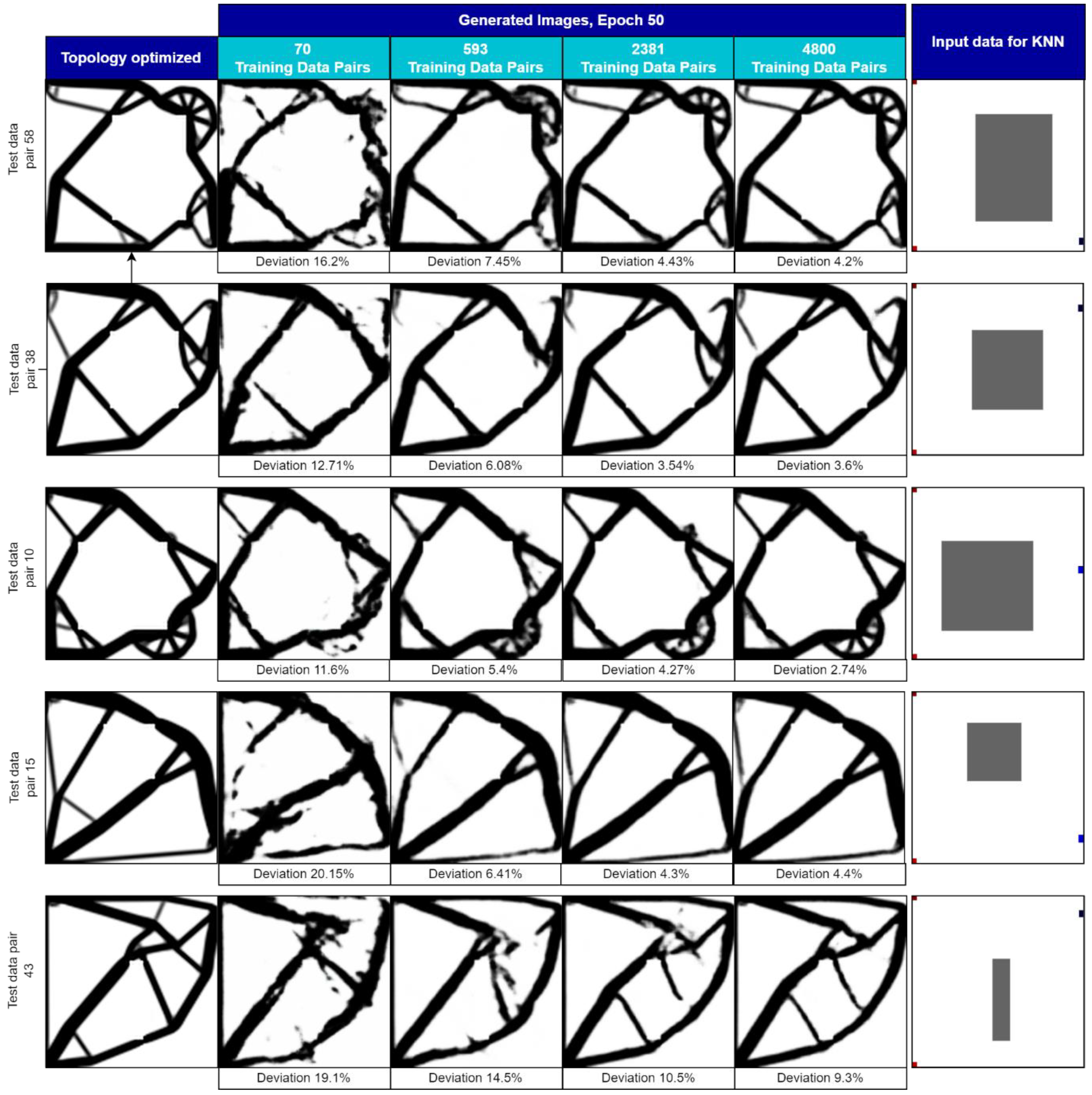
In the sixth step, 10,000 training data pairs were used with a rigorous test involving a highly complex problem. Despite using a relatively small number of training data pairs compared to the vast number of possible combinations, the model was trained on this challenging dataset. Consequently, the model faced significant difficulties in generating complex TOs, resulting in the majority of generated images displaying disconnected regions from the rest of the geometry. While some meaningful generated images were observed, over half of them exhibited artefacts, indicating insufficient training data to handle the complexity of the problem effectively. It became evident that a more extensive and diverse training dataset was required to accurately capture and represent the intricacies of such complex TOs. Hence, in the seventh step, different numbers of training data pairs are created to analyze their impact on accuracy. Data pairs ranging from 70 to 4800 are generated for a constant point load in the positive or negative Y-direction along the outer right edge of the build space, and the model was trained using this varied dataset. Additionally, a passive element (variable rectangle) is introduced that freely varies within the build space, representing a manufacturing constraint where no material can be placed within this geometry. The rectangle could have different sizes and had a minimum distance of 15 elements from each edge of the build space to avoid unsolvable TO problems. The training data are approximately doubled for the models to gain further insights into the effects of training data on accuracy. Specifically, the dataset sizes comprised 70, 140, 287, 593, 1187, 2381, and 4800 training data pairs.
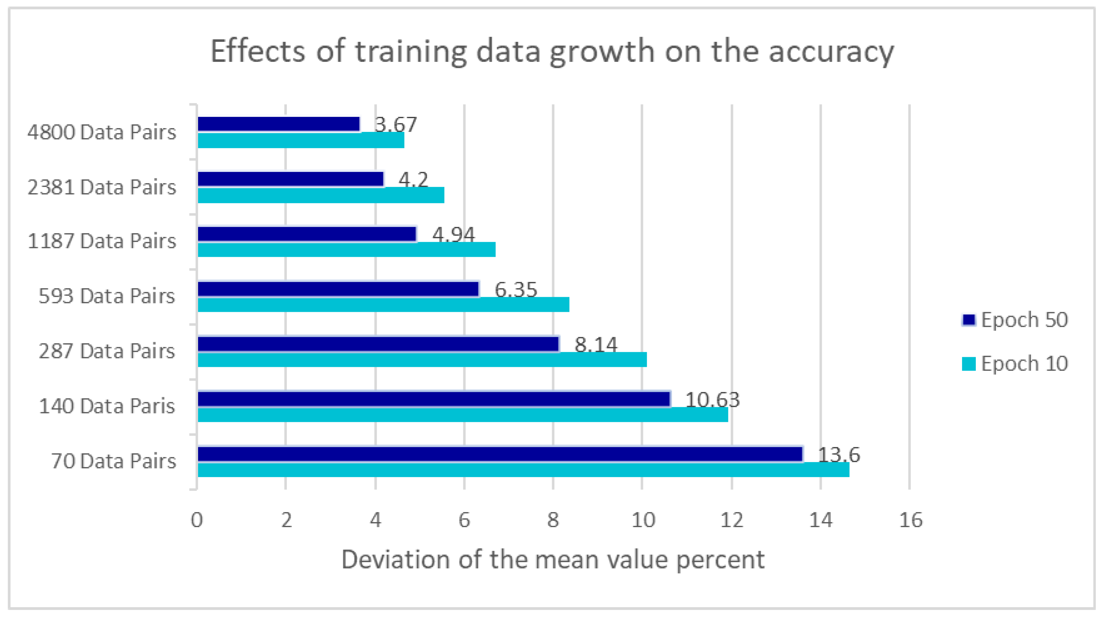
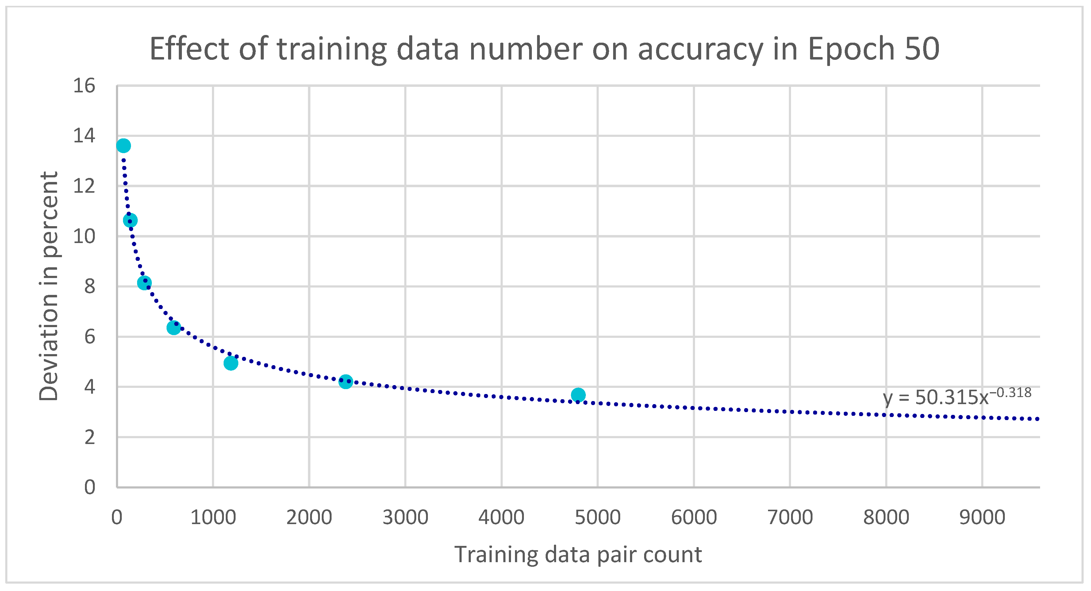
Figure 11 depicts the influence of training data growth at epoch values of 10 and 50 on accuracy. For the model with 70 data pairs, the deviation at epoch 50 is measured at 13.6%. Increasing the training data to 140 pairs significantly reduced this deviation to 10.63%. Further doubling the training data to 287 pairs results in another reduction in deviation, bringing it down to 8.14%. This apparent correlation between the number of data pairs and deviation is visually illustrated in Figure 8 and Figure 9. A 15% deviation reduction is achieved from 1187 data pairs to 2381 data pairs. Even with the doubling of data pairs from 2381 to 4800, a substantial 12.6% improvement in deviation is attained. Figure 11 complements Figure 12 by illustrating the accuracy course for the models up to epoch 50, represented with a linear training data pair plot. This visualization further highlights the consistent trend of improved accuracy as the number of training data pairs increases. These findings underscore the importance of sufficient training data in enhancing the accuracy of TO models for the additive manufacturing of individualized products. As demonstrated in this analysis, increasing the quantity of training data leads to a notable reduction in deviation and, consequently, more reliable and accurate TO results.
In addition to an increase in accuracy and a decrease in deviation with an increase in the dataset, it is also possible to observe, as shown in Figure 11 and Figure 12, that the trained machine learning model demonstrates the impact that different physical boundary conditions have on the model’s accuracy. Additionally, this will demonstrate the robustness of the machine learning model over a variety of boundary conditions. This leads to the idea of incorporating different boundary conditions and datasets within the trained ML model in a group, and hence, Section 3.3 becomes part of the discussion.
In contrast to the fifth model, the accuracy of the model has increased in the seventh model despite having a smaller number of training data pairs. Notably, this step has 150 times more possible variations, making it a more complex problem. However, it is essential to consider that this problem is less intricate, involving only one force, resulting in geometries that exhibit greater similarity. Figure 13 visually represents the differences between the individual models with varying numbers of training data pairs. It becomes evident that there are strong improvements in accuracy as the number of training data pairs increases. Nevertheless, achieving intricate structures remains challenging, even with 4800 training data pairs. The observed increase in accuracy, despite a smaller training dataset, can be attributed to the problem’s nature, where the complexity reduction and the geometries’ similarity allow for better performance with fewer training data pairs. However, the limitations in reproducing complex structures indicate that other factors may influence the accuracy of the model beyond the quantity of training data.
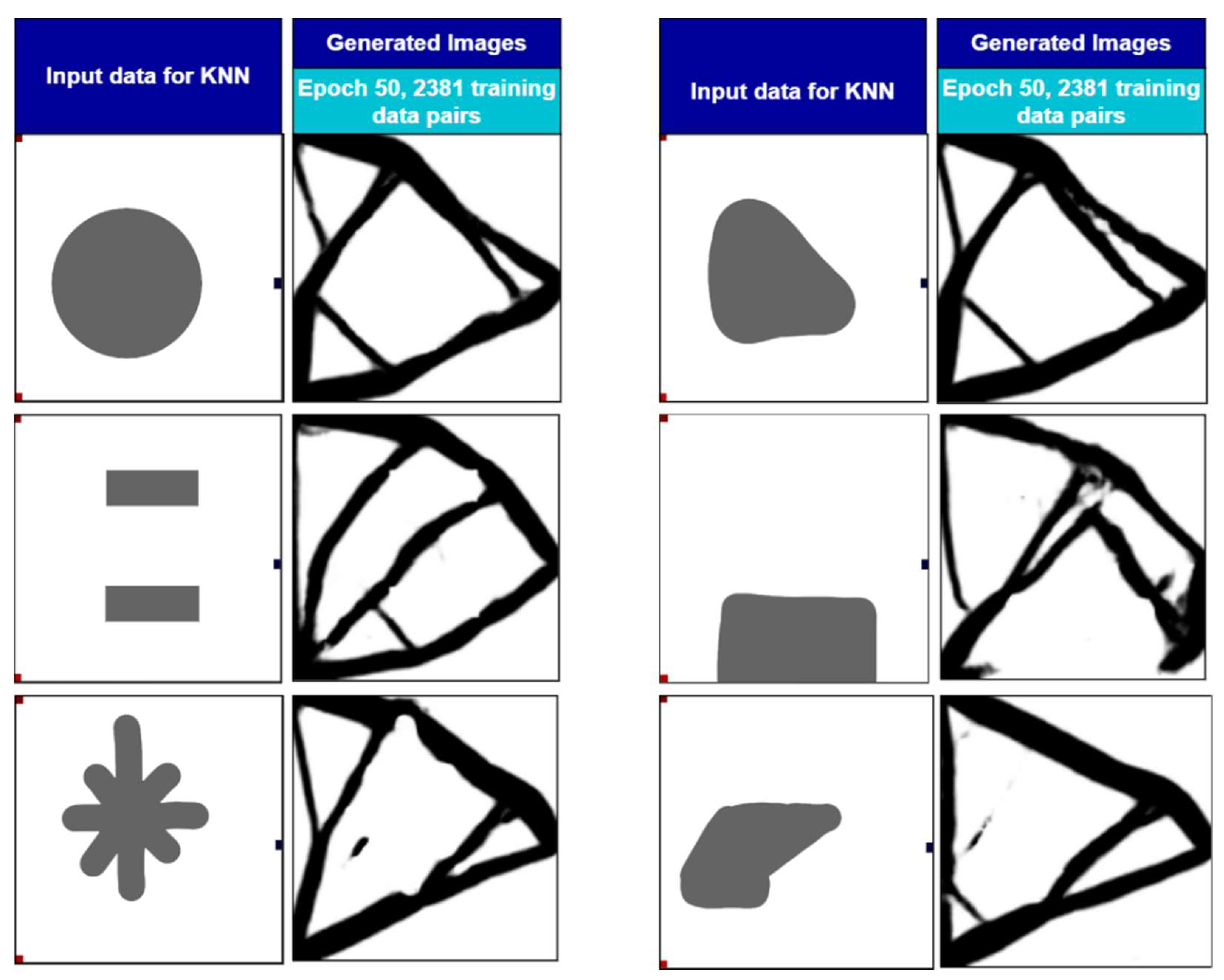
An intriguing observation emerged when the model was presented with the input data of geometries that deviated from the training dataset. Notably, the model had not been trained with these particular shapes, as shown in Figure 14. During the training process, the model was exclusively exposed to a variable-sized rectangular shape as a passive element, with the restriction that it should not touch the corners. However, on a test basis, various other shapes, including circles and free forms, were provided as input to the model. Surprisingly, the model produced results that maintained a clear area around the freeform geometry, but the outcomes were imperfect. Although the results were not flawless, the model’s behavior in adhering to the manufacturing restriction for untrained shapes demonstrates its potential for practical applications in additive manufacturing, particularly in ensuring design compliance with specific manufacturing constraints. This intriguing behavior opens up new possibilities for exploring the adaptability and robustness of the ML model in handling diverse geometries and manufacturing scenarios and can be changed as per the requirements of the additive manufacturing process. The training of the model can be further enhanced by incorporating different shapes of constraints.

3.2. Validation

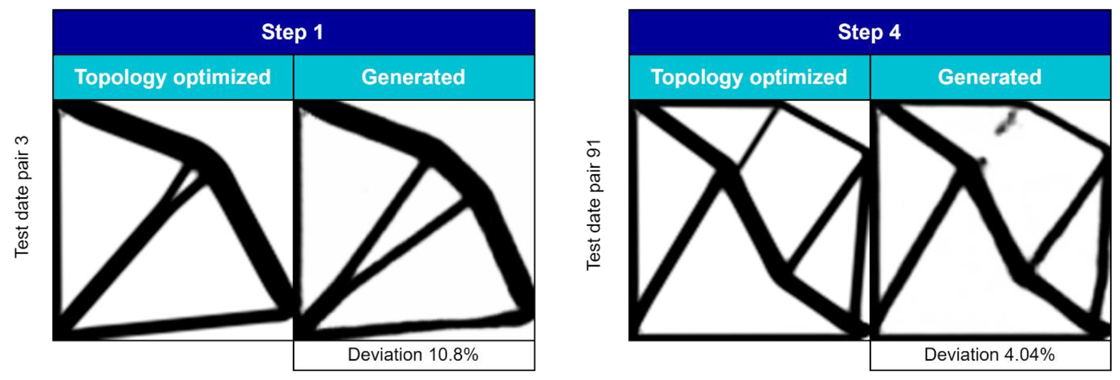
The validation process involved a comparison of image data, where a pixel-by-pixel analysis was conducted to examine the differences between the generated and TO images. In TO, multiple solutions can exist for a given problem, and validating these solutions solely based on image data comparison does not provide a comprehensive understanding of the results. As a consequence, images with high deviations still required visual inspection afterward. The advantage of this validation method lies in its high throughput and efficiency, as it only necessitates comparing values within the image matrices.
Image data comparison was employed for validation purposes. Discrepancies between the generated images and the topology-optimized images were examined pixel-by-pixel. While this approach provides a valuable overall assessment of the quality of the findings, it is important to note that, occasionally, unrelated structures may also exhibit slight variations. Although such instances are infrequent, they can still be observed, as demonstrated in Figure 15 (on the right). Despite the relatively small deviation of only 4.04%, the structure in question is not optimal and contains unrelated components. Conversely, images created with significant deviations may also encompass structurally meaningful elements. An example of such a structure featuring relevant architectural components is displayed in Figure 15 (on the left). Notably, the degree of variance in this instance is 10.8%. Given the possible solutions in topology optimization, it is important to acknowledge that comprehensive validation via image data comparison may not encompass the entire spectrum of meaningful information. In cases where images exhibit high levels of variance, visual inspection becomes necessary after applying the validation procedure. Because this validation method only compares the values within the image matrices, it offers the advantage of high throughput within a brief timeframe. While a qualitative assessment could involve comparing minimal compliance, implementing such an approach would necessitate the development or utilization of a 2D finite element method (FEM) analysis tool. This tool would require the transfer of restraints and applied forces from generating training data. However, due to scheduling constraints, creating such a tool was not feasible. For more clarity, it should be noted that the validation conducted in this study is limited to image-based comparisons between the ML-generated designs and traditional topology-optimized structures. Due to time constraints, mechanical validation, such as FEM analysis, was not performed. Future studies will include FEM-based validation to assess the mechanical performance of the generated topologies in terms of compliance, safety factors, and other relevant criteria.

3.3. Combination of Models to Improve Results

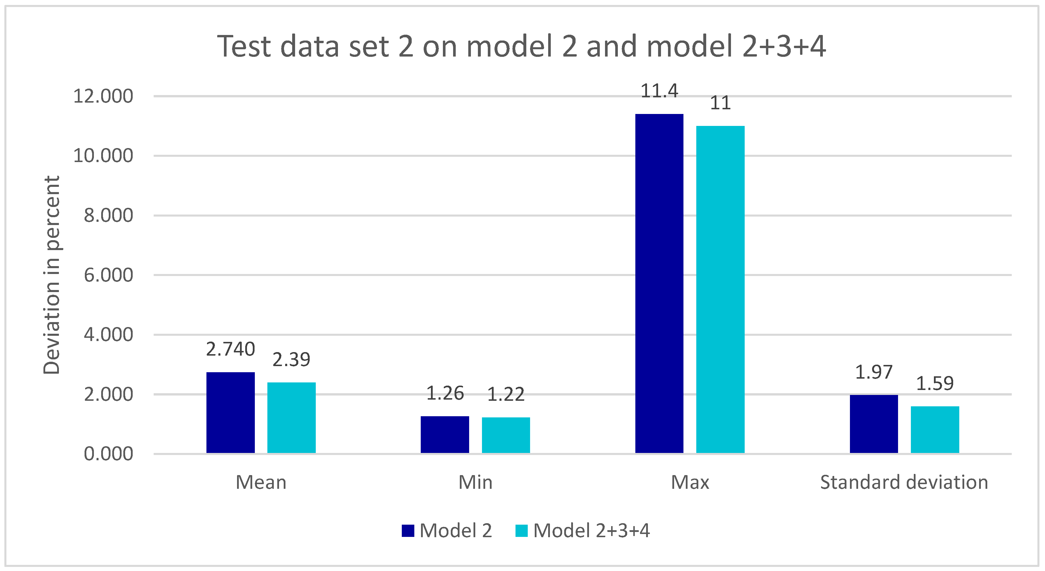
The second model demonstrated significant improvements in generating TO structures compared to the first model. It excels in translating color-coded images into TO structures, leading to a notable reduction in artefacts. However, small artefacts prevent a fully automated one-to-one conversion of the generated images into structures despite improvements. Interestingly, the accuracy of the second model increases significantly when combining the training data from Models 2, 3, and 4. Ensemble learning involves training multiple models (sub-models) and then combining their predictions to make a final decision. The idea behind ensemble methods is that different models may capture different aspects of the data, and by combining their strengths, the overall performance can be enhanced. Although the parameters differ between these steps, the second step benefits from the additional data from Steps 3 and 4. This combined model, named model 2+3+4, shows a percentage improvement in the categories of mean value, maximum value, and standard deviation of the mean value, as depicted in Figure 16. Furthermore, Figure 17 visually illustrates the improvement of two generated images when using the combined model, with most of the strong artefacts disappearing. As a result, on the left side, two generated photos exhibit prominent artefacts attributed to Model 2. Despite various issues across the training datasets, these artefacts are mostly mitigated in the combined model. When Model 3 or Model 4 are independently tested using the test data from Step 2, the deviation increases to 20.25% and 14.9%, respectively. Given that the generated test images contain only two relevant artefacts, the combined Model 2+3+4 can be considered a viable alternative to the iterative topology optimization used in Step 2. However, this approach presents challenges due to the existence of artefacts, making the direct transformation of the produced images into feasible structures more arduous. As a design template, this model is highly suitable due to the low and distinguishable artefacts from the relevant structures. Similarly, Models 3 and 4 are combined, but the results are unreliable enough to be used as a design template.

3.4. Algorithm Extension to Additive Manufacturing (AM)

As the trained model needs to be utilized for AM, all the possible restrictions related to AM must also be added. Model 7 successfully included the manufacturing restriction of the passive elements, which proved beneficial for algorithm training. Implementing further restrictions, such as a minimum wall thickness, would likely enhance the AI’s precision even more. By introducing a minimum wall thickness, the model can eliminate very fine structures, which were a primary issue in the generated structures of some models. As a result, the models’ accuracy would increase. Therefore, it is foreseeable that AI models will also adhere to additional manufacturing constraints given in the training data. These constraints will likely improve the precision since they further limit the solution space.
AM is a fast-growing technological trend in both commercial and residential sectors. AM methods, particularly laser powder bed fusion (LPBF), enable the production of complicated geometries such as organic structures, topology-optimized structures, and fill structures such as honeycombs [60,61,62]. Adhering to construction guidelines, such as maintaining a minimum wall thickness, is critical to avoiding complications such as warping or breaking during printing. Optimizing component orientation to reduce support structures is also very important. Despite potential obstacles such as shrinkage, residual tensions, and anisotropic characteristics, the benefits of AM make it ideal for producing prototypes and small batches of complicated parts. In the traditional design process of a TO product, relevant parameters are derived from requirements, and the design space is modeled in CAD. The TO algorithm is set up with constraints, and the optimization process can take varying amounts of time [29,30]. If necessary, adjustments are made, and the design is validated using finite element method (FEM) analysis before manufacturing. An alternative approach to design involves using ML models trained with various problems and their corresponding training data. This ML-driven tentative approach bypasses the complex process of TO, allowing the design process to begin directly with a design template. This alternative approach increases efficiency and enables a higher throughput of individual products. A comparison is shown in Figure 18.

4. Practical Application of TO and ML

In this section, we will examine the practical implications of our approach to the utilization of image super-resolution models in TO. Through the utilization of our models, we can demonstrate that the suggested method has the potential to greatly speed up the process of TO in a wide range of structural issues. In particular, the flexibility of our technique is particularly notable. We demonstrate that it can generalize to a wide range of problem circumstances and structures, while simultaneously lowering the number of iterative computations necessary for convergence by a significant amount. This approach can be extended to various examples. For instance, the model can be used to optimize patient-specific implants [63], similar to conventional TO. With our model, using the build space and passive elements (voids) we described in our study will also add leverage for AM. Furthermore, there is another class of structures called lattice structures with functional grading [64]. This ML model can also be used to further improve the properties of such functionally graded lattice structures, as well as the incorporation of TO and ML, in less time. Similarly, the feature discussed in our study is lightweight and the strength of the structure, which is a very important perspective of any TO application, is also present in the literature [65]. Moreover, the studies performed to use TO for finding build directions [66] and self-supporting structures [67] can be well-covered with little modification in our model. In future work, the constraint part can change to different types of constraints, such as the buckling of the structure or its elements [68]. As highlighted above, constraint and passive elements are vital in the usage of this model in AM applications. As TO has wide areas of application ranging from aerospace to fluid mechanics [69,70], there is no doubt that this study can help accelerate the process of TO with the help of ML. Recently, J. Lim et al. published a similar approach, in which TO is achieved based on deep learning with super-resolution for images [56]. S. Shin et al. [20] offer a very detailed assessment of the application of machine learning (ML) in TO, including deep learning, and emphasize important gains that have been realized using such an approach. Consequently, several studies have been conducted to enable optimization that is both effective and quick by utilizing machine learning in conjunction with TO.

5. Possible Future Work

The approach and models used in this study can be extended to three-dimensional structures by explaining the wall thickness with comparable expected results. Promising results from this study support the potential success of this approach when applied to the individual planes of 3D structures. Converting color-coded images into multidimensional matrices can be done easily. However, addressing artefacts distributed across different layers in 3D structures poses a challenge. Developing a separate neural network to recognize and remove these artefacts could enhance the accuracy of the designs. With these advancements, the ML-driven TO approach shows high promise for improving efficiency and effectiveness in a wide range of engineering applications.
To further refine our approach, future studies may explore the integration of specialized algorithms to prevent common topology optimization artefacts, such as checkerboard patterns and disconnected regions. This will involve the development of advanced regularization techniques that can be smoothly incorporated into our existing machine learning framework, thereby enhancing the structural integrity and functionality of the optimized designs. Another possibility for future work could be the application of FEM analysis or similar mechanical validation methods to ensure that the ML-generated topologies meet essential design criteria, such as compliance, load-bearing capacity, and safety factors. This would provide further validation of the generated designs and confirm their mechanical reliability in practical engineering applications.

6. Conclusions

This work delves into the exploration of the ML model’s potential as a substitute for iterative topology optimization. This investigation centers around a parameterized and topology-optimized product, illustrated through the case study of a cantilever. The following conclusions can be drawn from this article:
  • The work encompasses the development of code for training data generation, the utilization of software for topology optimization, and the implementation of an AI algorithm. Specifically, the adopted AI algorithm is a conditional generative adversarial network (cGAN) known as Pix2Pix. This cGAN was trained using pairs of data, where each pair comprises color-coded images containing the cantilever’s parameters and the corresponding topology-optimized target structures. Throughout this study, diverse models for generating topology-optimized cantilevers were conceived and subsequently investigated. Moreover, the analysis extended to exploring the relationship between the quantity of training data and the model’s accuracy.
  • The developed model uses an ML-trained model to substitute or streamline the traditional iterative phases of the TO, which shortens the development cycle and decreases overall development costs.
  • Parameters subject to parameterization in this study encompassed the load type, force application location, quantity of applied forces, force amplitude, direction of force application, dimensions of the construction space, and manufacturing constraints that specify that regions are to be preserved and free. Test data pairs that remained undisclosed to the algorithm were employed for validation purposes.
  • The model displaying the highest accuracy is the third model for all potential variations. This model focuses on varying the parameters related to the positions of two applied forces along the opposite edge of the cantilever’s restraint. The varying parameters in the seventh model include a force that varies in location and direction and a color-coded rectangle that traverses the construction space and delineates areas where no material can be placed. This shows the robust nature of the trained algorithm. The combination of the model with sub-models is also a tested method to increase the accuracy of the results. Models 2, 3, and 4 with sub-models also prove the robust nature of the algorithm.
  • There are several artefacts in the ML model compared to TO. Dependability of up to 91% was reached for artefact-free structures. However, the resulting artefact-filled pictures may be used extremely dependably as design templates. Additionally, Step 7, which was used to evaluate production restrictions, has always complied with and performed quite dependably with constraints.

Author Contributions

Conceptualization, A.U., L.H. and K.A. (Karim Asami); methodology, A.U. and L.H.; software, L.H. and K.B.; validation, A.U., K.A. (Karim Asami) and T.R.; formal analysis, A.U. and K.A. (Karim Asami); investigation, A.U.; resources, K.B. and K.A. (Kashif Azher); data curation, A.U and K.A. (Kashif Azher); writing—original draft preparation, A.U.; writing—review and editing, A.U, K.A. (Karim Asami), T.R and K.A. (Kashif Azher); visualization, K.B. and L.H.; supervision, K.B. and C.E.; project administration, K.B. and C.E.; funding acquisition, C.E. All authors have read and agreed to the published version of the manuscript.

Funding

The first author Abid Ullah works under the REDI Program, a project that has received funding from the European Union’s Horizon 2020 research and innovation program under the Marie Skłodowska-Curie grant agreement no. 101034328. This paper reflects only the author’s view and the Research Executive Agency is not responsible for any use that may be made of the information it contains. Publishing fees are supported by the Funding Programme Open Access Publishing of the Hamburg University of Technology (TUHH).

Data Availability Statement

Dataset available on request from the authors.

Conflicts of Interest

Author Lukas Holtz was employed by the company Teccon Consulting & Engineering GmbH. The remaining authors declare that the research was conducted in the absence of any commercial or financial relationships that could be construed as a potential conflict of interest.

References

  1. Zhu, J.; Zhou, H.; Wang, C.; Zhou, L.; Yuan, S.; Zhang, W. A review of topology optimization for additive manufacturing: Status and challenges. Chin. J. Aeronautics 2021, 34, 91–110. [Google Scholar] [CrossRef]
  2. Sepasgozar, S.M.E.; Shi, A.; Yang, L.; Shirowzhan, S.; Edwards, D.J. Additive Manufacturing Applications for Industry 4.0: A Systematic Critical Review. Buildings 2020, 10, 231. [Google Scholar] [CrossRef]
  3. Ullah, A.; Ur Rehman, A.; Salamci, M.U.; Pıtır, F.; Liu, T. The influence of laser power and scanning speed on the microstructure and surface morphology of Cu2O parts in SLM. Rapid Prototyp. J. 2022, 28, 1796–1807. [Google Scholar] [CrossRef]
  4. Vahedi Nemani, A.; Ghaffari, M.; Sabet Bokati, K.; Valizade, N.; Afshari, E.; Nasiri, A. Advancements in Additive Manufacturing for Copper-Based Alloys and Composites: A Comprehensive Review. J. Manuf. Mater. Process. 2024, 8, 54. [Google Scholar] [CrossRef]
  5. Granse, T.; Pfeffer, S.; Springer, P.; Refle, O.; Leitl, S.; Neff, M.; Duffner, E.; Dorneich, A.; Fritton, M. Manufacturing of individualized sensors: Integration of conductive elements in additively manufactured PBT parts and qualification of functional sensors. Prog. Addit. Manuf. 2024, 9, 273–283. [Google Scholar] [CrossRef]
  6. Hegab, H.; Khanna, N.; Monib, N.; Salem, A. Design for sustainable additive manufacturing: A review. Sustain. Mater. Technol. 2023, 35, e00576. [Google Scholar] [CrossRef]
  7. Mangla, S.K.; Kazancoglu, Y.; Sezer, M.D.; Top, N.; Sahin, I. Optimizing fused deposition modelling parameters based on the design for additive manufacturing to enhance product sustainability. Comput. Ind. 2023, 145, 103833. [Google Scholar] [CrossRef]
  8. Sigmund, O. A 99 line topology optimization code written in Matlab. Struct. Multidiscip. Optim. 2001, 21, 120–127. [Google Scholar] [CrossRef]
  9. Andreassen, E.; Clausen, A.; Schevenels, M.; Lazarov, B.S.; Sigmund, O. Efficient topology optimization in MATLAB using 88 lines of code. Struct. Multidiscip. Optim. 2011, 43, 1–16. [Google Scholar] [CrossRef]
  10. Talischi, C.; Paulino, G.H.; Pereira, A.; Menezes, I.F.M. PolyTop: A Matlab implementation of a general topology optimization framework using unstructured polygonal finite element meshes. Struct. Multidiscip. Optim. 2012, 45, 329–357. [Google Scholar] [CrossRef]
  11. Kumar, P. TOPress: A MATLAB implementation for topology optimization of structures subjected to design-dependent pressure loads. Struct. Multidiscip. Optim. 2023, 66, 97. [Google Scholar] [CrossRef]
  12. Hoang, V.-N.; Nguyen, N.-L.; Tran, D.Q.; Vu, Q.-V.; Nguyen-Xuan, H. Data-driven geometry-based topology optimization. Struct. Multidiscip. Optim. 2022, 65, 69. [Google Scholar] [CrossRef]
  13. Dugast, F.; To, A.C. Topology optimization of support structures in metal additive manufacturing with elastoplastic inherent strain modeling. Struct. Multidiscip. Optim. 2023, 66, 105. [Google Scholar] [CrossRef]
  14. Zou, J.; Zhang, Y.; Feng, Z. Topology optimization for additive manufacturing with self-supporting constraint. Struct. Multidiscip. Optim. 2021, 63, 2341–2353. [Google Scholar] [CrossRef]
  15. Ibhadode, O.; Zhang, Z.; Sixt, J.; Nsiempba, K.M.; Orakwe, J.; Martinez-Marchese, A.; Ero, O.; Shahabad, S.I.; Bonakdar, A.; Toyserkani, E. Topology optimization for metal additive manufacturing: Current trends, challenges, and future outlook. Virtual Phys. Prototyp. 2023, 18, e2181192. [Google Scholar] [CrossRef]
  16. Miki, T.; Yamada, T. Topology optimization considering the distortion in additive manufacturing. Finite Elem. Anal. Des. 2021, 193, 103558. [Google Scholar] [CrossRef]
  17. Zou, J.; Xia, X. Topology optimization for additive manufacturing with strength constraints considering anisotropy. J. Comput. Des. Eng. 2023, 10, 892–904. [Google Scholar] [CrossRef]
  18. Parvizian, J.; Düster, A.; Rank, E. Topology optimization using the finite cell method. Optim. Eng. 2012, 13, 57–78. [Google Scholar] [CrossRef]
  19. Gao, J.; Xiao, M.; Zhang, Y.; Gao, L. A Comprehensive Review of Isogeometric Topology Optimization: Methods, Applications and Prospects. Chin. J. Mech. Eng. 2020, 33, 87. [Google Scholar] [CrossRef]
  20. Shin, S.; Shin, D.; Kang, N. Topology optimization via machine learning and deep learning: A review. J. Comput. Des. Eng. 2023, 10, 1736–1766. [Google Scholar] [CrossRef]
  21. Liu, J.; Gaynor, A.T.; Chen, S.; Kang, Z.; Suresh, K.; Takezawa, A.; Li, L.; Kato, J.; Tang, J.; Wang, C.C.L.; et al. Current and future trends in topology optimization for additive manufacturing. Struct. Multidiscip. Optim. 2018, 57, 2457–2483. [Google Scholar] [CrossRef]
  22. Senck, S.; Rendl, S.; Kastner, J.; Ehrenfellner, P.; Happl, M.; Reiter, M. Simulation-based optimization of microcomputed tomography inspection parameters for topology-optimized aerospace brackets. In AIAA SCITECH 2022 Forum; American Institute of Aeronautics and Astronautics: Reston, VA, USA, 2021. [Google Scholar]
  23. Zegard, T.; Paulino, G.H. Bridging topology optimization and additive manufacturing. Struct. Multidiscip. Optim. 2016, 53, 175–192. [Google Scholar] [CrossRef]
  24. Chaturvedi, S.; Thakur, A.; Srivastava, P. Refining Language Translator Using Indepth Machine Learning Algorithms. In Proceedings of the 2024 11th International Conference on Reliability, Infocom Technologies and Optimization (Trends and Future Directions) (ICRITO), Noida, India, 14–15 March 2024; pp. 1–6. [Google Scholar]
  25. Henrique, B.M.; Sobreiro, V.A.; Kimura, H. Literature review: Machine learning techniques applied to financial market prediction. Expert Syst. Appl. 2019, 124, 226–251. [Google Scholar] [CrossRef]
  26. Zerouaoui, H.; Idri, A. Reviewing Machine Learning and Image Processing Based Decision-Making Systems for Breast Cancer Imaging. J. Med. Syst. 2021, 45, 8. [Google Scholar] [CrossRef] [PubMed]
  27. Soori, M.; Arezoo, B.; Dastres, R. Artificial intelligence, machine learning and deep learning in advanced robotics, a review. Cogn. Robot. 2023, 3, 54–70. [Google Scholar] [CrossRef]
  28. Jin, H.; Zhang, E.; Espinosa, H.D. Recent Advances and Applications of Machine Learning in Experimental Solid Mechanics: A Review. Appl. Mech. Rev. 2023, 75, 061001. [Google Scholar] [CrossRef]
  29. Ciccone, F.; Bacciaglia, A.; Ceruti, A. Optimization with artificial intelligence in additive manufacturing: A systematic review. J. Braz. Soc. Mech. Sci. Eng. 2023, 45, 303. [Google Scholar] [CrossRef]
  30. Weichert, D.; Link, P.; Stoll, A.; Rüping, S.; Ihlenfeldt, S.; Wrobel, S. A review of machine learning for the optimization of production processes. Int. J. Adv. Manuf. Technol. 2019, 104, 1889–1902. [Google Scholar] [CrossRef]
  31. Xiong, Y.; Tang, Y.; Zhou, Q.; Ma, Y.; Rosen, D.W. Intelligent additive manufacturing and design: State of the art and future perspectives. Addit. Manuf. 2022, 59, 103139. [Google Scholar] [CrossRef]
  32. Lei, X.; Liu, C.; Du, Z.; Zhang, W.; Guo, X. Machine learning-driven real-time topology optimization under moving morphable component-based framework. J. Appl. Mech. Trans. ASME 2019, 86, 011004. [Google Scholar] [CrossRef]
  33. Woldseth, R.V.; Aage, N.; Bærentzen, J.A.; Sigmund, O. On the use of artificial neural networks in topology optimisation. Struct. Multidiscip. Optim. 2022, 65, 294. [Google Scholar] [CrossRef]
  34. Abueidda, D.W.; Koric, S.; Sobh, N.A. Topology optimization of 2D structures with nonlinearities using deep learning. Comput. Struct. 2020, 237, 106283. [Google Scholar] [CrossRef]
  35. Qian, C.; Ye, W. Accelerating gradient-based topology optimization design with dual-model artificial neural networks. Struct. Multidiscip. Optim. 2021, 63, 1687–1707. [Google Scholar] [CrossRef]
  36. Wu, C.; Luo, J.; Zhong, J.; Xu, Y.; Wan, B.; Huang, W.; Fang, J.; Steven, G.P.; Sun, G.; Li, Q. Topology optimisation for design and additive manufacturing of functionally graded lattice structures using derivative-aware machine learning algorithms. Addit. Manuf. 2023, 78, 103833. [Google Scholar] [CrossRef]
  37. Hassan, A.M.; Biaggi, A.P.; Asaad, M.; Andejani, D.F.; Liu, J.; Offodile2nd, A.C.; Selber, J.C.; Butler, C.E. Development and Assessment of Machine Learning Models for Individualized Risk Assessment of Mastectomy Skin Flap Necrosis. Ann. Surg. 2023, 278, e123–e130. [Google Scholar] [CrossRef]
  38. Maksum, Y.; Amirli, A.; Amangeldi, A.; Inkarbekov, M.; Ding, Y.; Romagnoli, A.; Rustamov, S.; Akhmetov, B. Computational Acceleration of Topology Optimization Using Parallel Computing and Machine Learning Methods—Analysis of Research Trends. J. Ind. Inf. Integr. 2022, 28, 100352. [Google Scholar] [CrossRef]
  39. Sun, Z.; Wang, Y.; Liu, P.; Luo, Y. Topological dimensionality reduction-based machine learning for efficient gradient-free 3D topology optimization. Mater. Des. 2022, 220, 110885. [Google Scholar] [CrossRef]
  40. Deng, C.; Wang, Y.; Qin, C.; Fu, Y.; Lu, W. Self-directed online machine learning for topology optimization. Nat. Commun. 2022, 13, 388. [Google Scholar] [CrossRef]
  41. Herrero-Pérez, D.; Picó-Vicente, S.G.; Martínez-Barberá, H. Efficient distributed approach for density-based topology optimization using coarsening and h-refinement. Comput. Struct. 2022, 265, 106770. [Google Scholar] [CrossRef]
  42. Träff, E.A.; Sigmund, O.; Aage, N. Topology optimization of ultra high resolution shell structures. Thin-Walled Struct. 2021, 160, 107349. [Google Scholar] [CrossRef]
  43. Puri, D.; Sihag, P.; Thakur, M.S. A review: Aeration efficiency of hydraulic structures in diffusing DO in water. MethodsX 2023, 10, 102092. [Google Scholar] [CrossRef] [PubMed]
  44. Zhu, C. Chapter 1—Introduction to machine reading comprehension. In Machine Reading Comprehension; Zhu, C., Ed.; Elsevier: Amsterdam, The Netherlands, 2021; pp. 3–26. [Google Scholar]
  45. What Is the “k-Nearest Neighbors’ Algorithm”? | IBM. Available online: https://www.ibm.com/de-de/topics/knn (accessed on 22 September 2024).
  46. Mirza, M.; Osindero, S. Conditional Generative Adversarial Nets. arXiv 2014, arXiv:1411.1784. [Google Scholar]
  47. What Is a Conditional Generative Adversarial Network (cGAN)? DataScientest. Available online: https://datascientest.com/en/what-is-a-conditional-generative-adversarial-network-cgan (accessed on 23 September 2024).
  48. Cascella, M.; Scarpati, G.; Bignami, E.G.; Cuomo, A.; Vittori, A.; Di Gennaro, P.; Crispo, A.; Coluccia, S. Utilizing an artificial intelligence framework (conditional generative adversarial network) to enhance telemedicine strategies for cancer pain management. J. Anesth. Analg. Crit. Care 2023, 3, 19. [Google Scholar] [CrossRef] [PubMed]
  49. El-Brawany, M.A.; Adel Ibrahim, D.; Elminir, H.K.; Elattar, H.M.; Ramadan, E.A. Artificial intelligence-based data-driven prognostics in industry: A survey. Comput. Ind. Eng. 2023, 184, 109605. [Google Scholar] [CrossRef]
  50. Erickson, B.J.; Kitamura, F. Magician’s Corner: 9. Performance Metrics for Machine Learning Models. Radiol. Artif. Intell. 2021, 3, e200126. [Google Scholar] [CrossRef]
  51. Joglekar, A.; Chen, H.; Kara, L.B. DMF-TONN: Direct Mesh-free Topology Optimization using Neural Networks. Eng. Comput. 2024, 40, 2227–2240. [Google Scholar] [CrossRef]
  52. Zhang, W.; Wang, Y.; Youn, S.-K.; Guo, X. Machine learning powered sketch aided design via topology optimization. Comput. Methods Appl. Mech. Eng. 2024, 419, 116651. [Google Scholar] [CrossRef]
  53. Shishir, M.I.R.; Tabarraei, A. Multi–materials topology optimization using deep neural network for coupled thermo–mechanical problems. Comput. Struct. 2024, 291, 107218. [Google Scholar] [CrossRef]
  54. Xia, Z.; Zhang, H.; Zhuang, Z.; Yu, C.; Yu, J.; Gao, L. A machine-learning framework for isogeometric topology optimization. Struct. Multidiscip. Optim. 2023, 66, 83. [Google Scholar] [CrossRef]
  55. Lim, J.; Jung, K.; Jung, Y.; Kim, D.-N. Accelerating topology optimization using deep learning-based image super-resolution. Eng. Appl. Artif. Intell. 2024, 133, 108370. [Google Scholar] [CrossRef]
  56. Chi, H.; Zhang, Y.; Tang, T.L.E.; Mirabella, L.; Dalloro, L.; Song, L.; Paulino, G.H. Universal machine learning for topology optimization. Comput. Methods Appl. Mech. Eng. 2021, 375, 112739. [Google Scholar] [CrossRef]
  57. Isola, P.; Zhu, J.-Y.; Zhou, T.; Efros, A.A. Image-to-Image Translation with Conditional Adversarial Networks. In Proceedings of the 2017 IEEE Conference on Computer Vision and Pattern Recognition (CVPR), Honolulu, HI, USA, 21–26 July 2017; pp. 5967–5976. [Google Scholar]
  58. Mahdavi, M.; Abedjan, Z.; Castro Fernandez, R.; Madden, S.; Ouzzani, M.; Stonebraker, M.; Tang, N. Raha: A Configuration-Free Error Detection System. In Proceedings of the 2019 International Conference on Management of Data, Amsterdam, The Netherlands, 30 June 2019–5 July 2019; pp. 865–882. [Google Scholar]
  59. Epochs, Batch Size, Iterations—How Are They Important to Training AI and Deep Learning Models? SabrePC. Available online: https://www.sabrepc.com/blog/Deep-Learning-and-AI/Epochs-Batch-Size-Iterations (accessed on 21 September 2024).
  60. du Plessis, A.; Broeckhoven, C.; Yadroitsava, I.; Yadroitsev, I.; Hands, C.H.; Kunju, R.; Bhate, D. Beautiful and Functional: A Review of Biomimetic Design in Additive Manufacturing. Addit. Manuf. 2019, 27, 408–427. [Google Scholar] [CrossRef]
  61. King, W.E.; Anderson, A.T.; Ferencz, R.M.; Hodge, N.E.; Kamath, C.; Khairallah, S.A.; Rubenchik, A.M. Laser powder bed fusion additive manufacturing of metals; physics, computational, and materials challenges. Appl. Phys. Rev. 2015, 2, 041304. [Google Scholar] [CrossRef]
  62. Ullah, A.; Wu, H.; Ur Rehman, A.; Zhu, Y.; Liu, T.; Zhang, K. Influence of laser parameters and Ti content on the surface morphology of L-PBF fabricated Titania. Rapid Prototyp. J. 2021, 27, 71–80. [Google Scholar] [CrossRef]
  63. Park, S.M.; Park, S.; Park, J.; Choi, M.; Kim, L.; Noh, G. Design process of patient-specific osteosynthesis plates using topology optimization. J. Comput. Des. Eng. 2021, 8, 1257–1266. [Google Scholar] [CrossRef]
  64. Cheng, L.; Bai, J.; To, A.C. Functionally graded lattice structure topology optimization for the design of additive manufactured components with stress constraints. Comput. Methods Appl. Mech. Eng. 2019, 344, 334–359. [Google Scholar] [CrossRef]
  65. Kim, J.E.; Cho, N.K.; Park, K. Computational homogenization of additively manufactured lightweight structures with multiscale topology optimization. J. Comput. Des. Eng. 2022, 9, 1602–1615. [Google Scholar] [CrossRef]
  66. Bender, D.; Barari, A. Using 3D Density-Gradient Vectors in Evolutionary Topology Optimization to Find the Build Direction for Additive Manufacturing. J. Manuf. Mater. Process. 2023, 7, 46. [Google Scholar] [CrossRef]
  67. Barroqueiro, B.; Andrade-Campos, A.; Valente, R.A.F. Designing Self Supported SLM Structures via Topology Optimization. J. Manuf. Mater. Process. 2019, 3, 68. [Google Scholar] [CrossRef]
  68. Ferrari, F.; Sigmund, O. Towards solving large-scale topology optimization problems with buckling constraints at the cost of linear analyses. Comput. Methods Appl. Mech. Eng. 2020, 363, 112911. [Google Scholar] [CrossRef]
  69. Dørffler, P.; Jensen, L.; Wang, F.; Dimino, I.; Sigmund, O.; Jensen, C.; Wang, P.D.L.; Dimino, F.; Sigmund, I.; Topology, O. Topology Optimization of Large-Scale 3D Morphing Wing Structures. Actuators 2021, 10, 217. [Google Scholar] [CrossRef]
  70. Li, J.; Gao, L.; Ye, M.; Li, H.; Li, L. Topology optimization of irregular flow domain by parametric level set method in unstructured mesh. J. Comput. Des. Eng. 2022, 9, 100–113. [Google Scholar] [CrossRef]
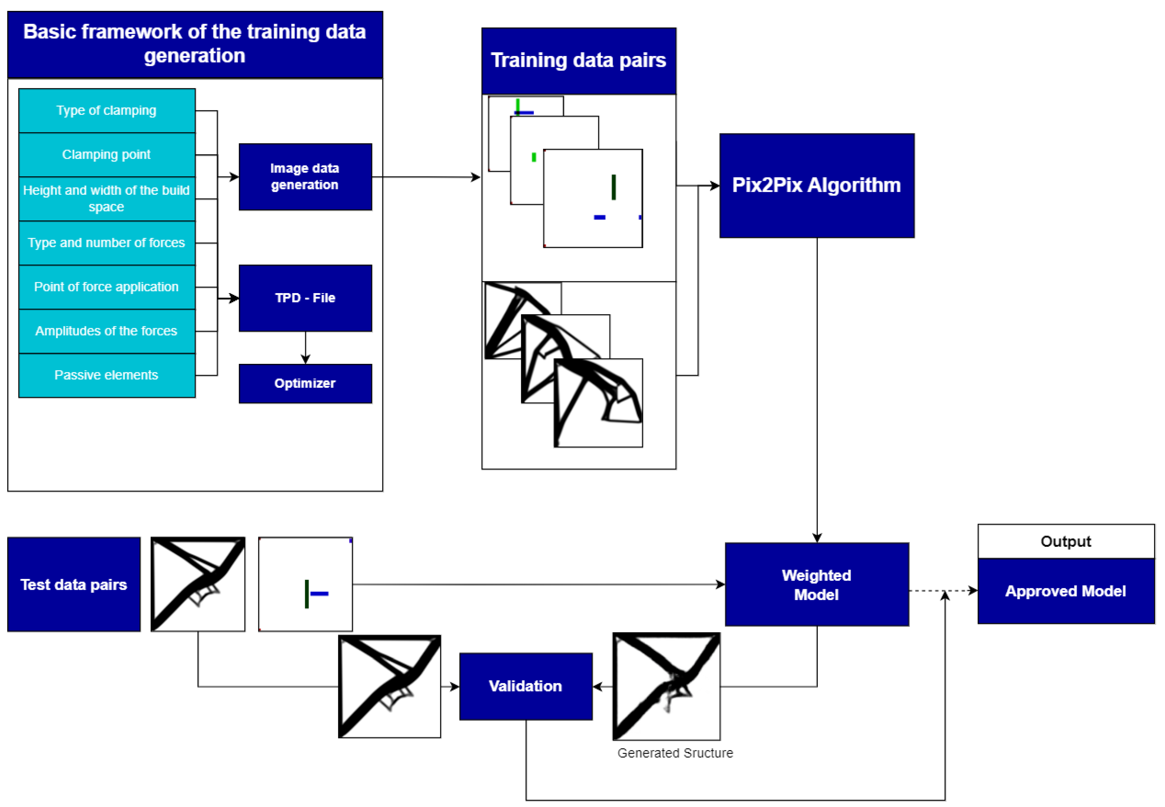
Figure 1. Illustration of the entire flowchart for this study with all the sub-steps involved.
Jmmp 08 00220 g001
Figure 2. Illustration of variable parameters and ToPy topology optimization workflow.
Jmmp 08 00220 g002
Figure 3. Graphical representation of steps for parametric model creation.
Jmmp 08 00220 g003
Figure 4. Epochs 10–80 compared to topology optimization.
Jmmp 08 00220 g004
Figure 5. Comparison between 100 and 500 epochs for Step 2.
Jmmp 08 00220 g005
Figure 6. Comparison between 10 and 100 epochs for Step 3.
Jmmp 08 00220 g006
Figure 7. Comparison between 10 and 100 epochs for Step 4.
Jmmp 08 00220 g007
Figure 8. Comparison of the epochs of the first two models in Step 1 and Step 2.
Jmmp 08 00220 g008
Figure 9. Comparison across the epochs of the models in the third and fourth steps.
Jmmp 08 00220 g009aJmmp 08 00220 g009b
Figure 10. Mean values compared across models with training data pairs 2000–5000.
Jmmp 08 00220 g010
Figure 11. The effects of training data growth on accuracy for Step 7 (epoch values of 10 and 50).
Jmmp 08 00220 g011
Figure 12. Correlation between the number of data pairs and deviation.
Jmmp 08 00220 g012
Figure 13. Differences between models with different numbers of training data pairs for Step 7 (70–4800).
Jmmp 08 00220 g013
Figure 14. Generation of images from input data for which the model was not trained (deviating shapes).
Jmmp 08 00220 g014
Figure 15. Validation problem based on pixel-to-pixel image data comparison.
Jmmp 08 00220 g015
Figure 16. Mean, minimum, maximum, and standard deviation of Model 2 and Model 2+3+4.
Jmmp 08 00220 g016
Figure 17. Model 2 and Model 2+3+4 in relation to the test data pair of Step 2.
Jmmp 08 00220 g017
Figure 18. Approach with a ML model for iteration substitution compared to a classical approach.
Jmmp 08 00220 g018
Table 1. Steps of model generation.
Steps Varying ParametersPossible VariationsNumber of Training Data
1Location of a point load Y+ (along the right outer edge).10130
2Location of a point load Y± (along the right outer edge).20265
3Location of two point loads X+Y+ (along the right outer edge).10,201700
4Location of two point loads X±Y± (along the right outer edge).40,8041500
5Location of two point loads X+Y± (Y± along the right outer edge) (X+ in the entire installation space).2,060,6025000
6Location and amplitude of a point load Y±. Location and length of two line loads X± Y± (Y± along the right outer edge) (line load X± vertical with length 5–30) (line load Y± horizontal with length).17.1 × 10910,000
7Location of a point load Y± (along the right outer edge). Passive element (variable rectangle) free in installation space.303,126,2504800
Disclaimer/Publisher’s Note: The statements, opinions and data contained in all publications are solely those of the individual author(s) and contributor(s) and not of MDPI and/or the editor(s). MDPI and/or the editor(s) disclaim responsibility for any injury to people or property resulting from any ideas, methods, instructions or products referred to in the content.