Multivariate Time-Series Classification of Critical Events from Industrial Drying Hopper Operations: A Deep Learning Approach

Abstract

In recent years, the advancement of Industry 4.0 and smart manufacturing has made a large amount of industrial process data attainable with the use of sensors installed on machines. This paper proposes an experimental predictive maintenance framework for an industrial drying hopper so that it can detect any unusual event in the hopper, which reduces the risk of erroneous fault diagnosis in the manufacturing shop floor. The experimental framework uses Deep Learning (DL) algorithms to classify Multivariate Time-Series (MTS) data into two categories—failure or unusual events and regular events—thus formulating the problem as a binary classification. The raw data extracted from the sensors contained missing values, suffered from imbalancedness, and were not labeled. Therefore, necessary preprocessing is performed to make them usable for DL algorithms and the dataset is self-labeled after defining the two categories precisely. To tackle the imbalanced data issue, data balancing techniques like ensemble learning with undersampling and Synthetic Minority Oversampling Technique (SMOTE) are used. Moreover, along with DL algorithms like Convolutional Neural Network (CNN) and Long Short-Term Memory (LSTM), Machine Learning (ML) algorithms like Support Vector Machine (SVM) and K-nearest neighbor (KNN) have also been used to perform a comparative analysis on the results obtained from these algorithms. The result shows that CNN is arguably the best algorithm for classifying this dataset into two categories and outperforms other traditional approaches as well as deep learning algorithms.

1. Introduction

The advancement of smart manufacturing, which combines information technology and operational technology, has enabled the collection and processing of large amounts of industrial process data [1]. This progress has been facilitated by the installation of numerous sensors in industrial equipment and machine tools on the shop floor, leading to an increase in available data. In many cases, these sensors record the activity of manufacturing machine tools over time, thus generating time-series data [2]. The analysis of time-series data has proven valuable in extracting meaningful events in smart manufacturing systems [3]. While time-series data can be found in various domains such as healthcare [4], climate [5], robotics [6], ecohydrology [7], stock markets [8], energy systems [9], etc., this paper focuses on the plastic processing industry as a case study within the manufacturing domain. A comprehensive review of time-series applications in manufacturing can be found in [10].

Sensors play a crucial role in the advancement of smart manufacturing systems, collecting data for various key variables over time, and forming Multivariate Time-Series (MTS) data. MTS data consists of multiple univariate time series (UTS), making MTS more complex due to the correlation between different variables. This paper focuses on the analysis of time-series data for classification, which involves identifying key events and their respective classes within a dataset. Classification models aim to categorize events based on specific patterns and assign them to corresponding categories. In MTS classification, the time series is divided into segments, each belonging to a category with distinct patterns.

Several algorithms have been developed to analyze MTS data. Traditional approaches used prior to the evolution of smart manufacturing include simple exponential smoothing [11], dynamic time warping [12,13], and autoregressive integrated moving averages [14]. Machine learning algorithms such as K-nearest neighbor [15], decision trees [16], and Support Vector Machine (SVM) [17] have also been employed. Some authors have combined the K-nearest neighbor with distance measures like DTW [18,19] or Euclidean distance [20,21]. It has been shown that ensembling different discriminant classifiers, such as SVM and nearest neighbor, along with other machine learning classifiers like decision trees and random forests, can yield better results than using nearest neighbor with dynamic time warping [12]. Traditional methods often struggle to identify important features within time-series data and fail to capture correlations between variables, leading to the false identification of categorical events [3]. Additionally, traditional approaches and machine learning algorithms face challenges in handling the massive volume of data. Deep learning, with its ability to handle large amounts of data using deep neural networks, has emerged as a solution for extracting meaningful features from MTS data.

Deep learning techniques, including various neural network algorithms, have gained significant attention in dealing with time-series problems, particularly MTS. Deep neural networks can learn patterns in the data by capturing the correlations between variables, surpassing traditional methods such as NN-DTW. While NN-DTW may perform well for a small number of variables, it becomes more complex as the number of variables increases [22]. In this paper’s case study, which involves twelve distinct temperature measures, deep neural networks are particularly relevant. The two most used neural networks are Convolutional Neural Networks (CNN) and Recurrent Neural Networks (RNN). CNNs are popular for computer vision tasks [23] and have been extensively applied to image recognition [24], natural language processing [25,26,27], image compression, and speech recognition [28]. CNNs have also been successful in handling MTS problems [3,22,29,30,31,32,33,34]. RNN, on the other hand, excels in sequential learning and performs well for univariate time series, but its application to MTS classification is limited [35]. However, it shows promise in dealing with time-series datasets containing missing values [36].

The research objective of this paper can be summarized as follows: studying the versatility of MTS analysis in the context of the drying hoppers mechanism and patterns of temperature profiles; understanding various parameters related to MTS and applying this understanding to analyze the current material drying process and various events associated with industrial drying hoppers; identifying different ways to address data labeling and imbalance data issues of real manufacturing data; evaluating the performance of a set of machine learning and deep neural network algorithms to classify the MTS data.

2. Background and State of the Art

2.1. Manufacturing Process

In the polymer processing industry, dryers play a crucial role in supplying dry-heated air that is blown upward through the to-be-dried material for several hours, while new undried, cold/moist material is continuously loaded on top of the dryer module, steadily moving downward through the dryer [37,38]. Modern drying hoppers are designed with a cylindrical body and a conical hole at the bottom. They ensure even temperature distribution and material flow by using spreader tubes to inject hot and dry air into the chamber. The process involves recirculating the hot air to continuously dry the material until the desired humidity level is achieved. Successful drying requires considering three main factors: drying time, drying temperature, and the dryness of circulating air. Drying time depends on the air temperature, initial dryness of the material, and target humidity. Higher air dryness and temperature accelerate the drying process, but excessively high temperatures may affect the material’s quality [39].

Monitoring the drying process is essential to avoid malfunctions. In a typical use case, a six-zoned temperature probe continuously measures the temperature at different heights within the vertically aligned drying chamber. This helps detect various disruptions in the drying process, such as over- or under-dried material and heater malfunctions [39]. The drying hopper consists of a drying hopper monitor and a regen wheel, both of which have a significant impact on polymer processing. The drying hopper monitor has eight temperature sensors, while the regen has three temperature sensors, including dew point temperature measurements for air delivery. Temperature sensors are used to measure these twelve temperatures over a period of one year for this specific case study. Figure 1 depicts a schematic of a drying hopper and sensor setup similar to the one used in this study.

The collected data are preprocessed by handling missing values, outliers, and extraneous cases. The dataset contains temperature readings for twelve temperature measures sampled at one-minute intervals over the course of a year. With a large amount of data available for the main temperature zones in the dryer/hopper system and additional zones in the regen and dryer regions, meaningful features can be extracted via real-time analysis. By analyzing these data in real time, the production planner can gain insights into the drying hopper’s performance and determine the necessary maintenance actions. Figure 2 shows the temperature profiles obtained from the sensors.

2.2. Time-Series Classification in Manufacturing—Algorithms

MTS has gained popularity across various domains for different purposes, including clinical diagnosis, weather prediction, stock price analysis, human motion detection, and fault detection in manufacturing processes. The manufacturing industry, in particular, has seen a significant increase in the use of MTS data due to the deployment of sensor systems in shop-floor machinery and machine tools. As a result, researchers in the manufacturing domain have focused on MTS analysis, such as classification, to address the challenges posed by these data. Temporal data mining, including MTS analysis, presents complexities arising from factors like spatial structure, time dependency, and correlations among variables. Consequently, researchers have been developing a variety of algorithms to handle these challenges. In this section, the current state of the art in MTS classification is explored from two perspectives: the traditional approach and the Artificial Neural Network (ANN) approach, specifically deep learning.

2.2.1. Traditional Algorithms

The K-nearest neighbor algorithm with Dynamic Time Warping (DTW) is commonly used as a benchmark for classifying MTS data. In ref. [40], the authors used the Large Margin Nearest Neighbor (LMNN) and DTW. Mahalanobis distance-based DTW is used to calculate the relations among variables using the Mahalanobis matrix and LMNN is used to learn the matrix by minimizing a renewed, non-differentiable cost function using the coordinate descent method. This method is compared with other similarity measure techniques of MTS and the authors claimed the superiority of their proposed method over other techniques. This technique is also used by the authors in [41]. DTW multivariate prototyping is used in evaluating scoring and assessment methods for virtual reality training simulators. It classifies the VR data as novice, intermediate, or expert where 1-NN DTW performed reasonably well; the only better algorithm for this case was RESNET, which is an advanced version of CNN [42]. Overall, using DTW as a dissimilarity measure among features of time series and adapting the nearest neighbor classifier in temporal data mining was very popular before the evolution of deep learning [43].

According to [38], there are two approaches that can be taken for MTS data using DTW. One approach involves summing up the DTW distances of UTS for each dimension of the MTS. The other approach calculates the distance between two time-series data by summing up the distances between each corresponding pair of time-series data. The authors argue that the traditional belief that these two methods are equivalent for MTS classification is not true, and their effectiveness varies depending on the specific case. They conducted experiments on a wide range of MTS datasets to support their claim and justify the use of different DTW approaches based on the problem at hand.

A parametric derivative DTW is another variant of the DTW used in temporal data mining. This technique combines two distances, which are the DTW distance between MTS and the DTW distance between derivatives of MTS. This new distance is used afterward for classification with nearest neighbor rules [44]. Using a template selection approach based on DTW so that the complex feature selection approach and domain knowledge can be avoided is another approach used for classifying MTS in [45]. Another variant of DTW is using DTW distance measured via integral transformation. Integral DTW is calculated as the value of DTW on the integrated time series. This technique combines the DTW and integral DTW with the 1-nearest neighbor classifier which shows no overfitting issue [46].

The symbolic representation of MTS is a traditional technique used for classification. It involves learning symbols using supervised learning algorithms, considering all elements of the time series simultaneously. Tree-based ensembles are utilized to detect interactions between UTS columns, enabling efficient handling of nominal and missing values [47]. Another symbolic representation technique is MrSEQL, which transforms the time-series data using symbolic aggregate approximation (SAX) [48] in the time domain and symbolic Fourier approximation (SFA) [49] in the frequency domain. Discriminative subsequences are extracted from the symbolic data and used as features for training a classification model [50,51]. WEASEL + MUSE is another approach that uses SFA transformation to create sequences of words. Feature selection is performed using a chi-squared model, and logistic regression is employed to learn the selected features. These symbolic representation methods provide alternatives to traditional DTW-based approaches in MTS classification tasks [52].

One of the most extensive research on traditional methods for both MTS and UTS can be found in [12], which highlights almost all of the above-mentioned traditional approaches in different categories like whole series similarity, phase-dependent intervals, phase-independent shapelets, dictionary-based classifiers, and combinations of transformations. This paper is a great resource for any time-series classification enthusiast to gain an overview of all the traditional methods. Another review paper that shows a brief overview of different classification approaches for MTS can be found in [51].

Machine learning algorithms, including both nonlinear techniques and ensemble learning techniques, have also been applied for time-series classification over the years. Traditional classifiers like Naïve Bayes, Decision Tree, and SVM are the most popular. Before using these algorithms, MTS data need to be converted into feature vector format. This is why the authors in [17] segmented the time series to obtain a qualitative description of each series and determined the frequent patterns. Afterward, the patterns that are highly discriminative between the classes are selected, and the data are transformed into vector format where the features are discriminative patterns.

2.2.2. Deep Learning Algorithms

ANN and deep learning, specifically Convolutional Neural Networks (CNN) and Recurrent Neural Networks (RNN) such as Long Short-Term Memory (LSTM), have gained significant popularity in the field of temporal data mining, particularly for time-series classification. CNN has been widely used with a 1D filter in the convolutional layer, allowing it to automatically discover and extract meaningful internal structures in input time series via convolution and pooling operations. This eliminates the need for manual feature engineering, which is typically required in traditional feature extraction methods [53]. The combination of CNN and LSTM, leveraging the strengths of both algorithms, has also shown excellent performance in time-series classification tasks. Researchers have proposed various versions and adaptations of these algorithms, each showing promising results in different case studies. The authors of [22,54] provided the summary and basics of the recent algorithmic advance in the use of deep learning for MTS classification.

The authors in [29] used a tensor scheme with multivariate CNN for the time-series classification where the model considers multivariate aspect and lag feature characteristics simultaneously. Four stages were used in CNN architecture, which are the input tensor transformations stage, univariate convolution stage, multivariate convolution stage, and fully connected stage. In this method, they used an image-like tensor scheme to encode the MTS data. This approach is taken because of the highly successful nature of CNN in computing the vision for image classification.

Deconvolution has been utilized in time-series data mining, in addition to the convolution operation. In a study [55], the authors employed a deconvolutional network combined with SAX discretization to learn the representation of MTS. This approach captured correlations using deconvolution and applied pooling operations for dimension reduction across each position of each variable. SAX discretization was used to extract a bag of features, resulting in improved classification accuracy. Another variation of CNN called dilated CNN treated MTS as an image and employed stacks of dilated and stridden convolutions to extract features across variables [31]. Among other CNN approaches, multi-channel deep CNN is widely utilized, where the model learns features from individual time series and combines them after the convolution and pooling stages. The combined features are then fed into a multilayer perceptron (MLP) for final classification [34].

In [56], the authors performed a principal component analysis for feature extraction and reduced the number of MTS variables to two so that they could identify the most useful two components in the machine. The time series are encoded into images using Gramian Angular field (GAF) and the images are used as input for the CNN. Another similar research can be found in [57] where three techniques of converting MTS data into images have been used and tested, which are GAF, Gramian Angular Difference Field (GADF), and Markov Transition Field (MTF). It has been found that different approaches to converting MTS into images do not affect the classification performance, and a simple CNN can outperform other approaches. In semiconductor manufacturing, it has been tested that MTS- CNN can successfully detect fault wafers with high accuracy, recall, and precision [3].

Combining CNN, LSTM, and DNN has been another highly used approach over the years. In [58], the authors proposed a combined architecture abbreviated as CLDNN and applied it to large vocabulary tasks which outperformed three individual algorithms. A similar approach named MDDNN has been used to predict the class of a subsequence in terms of earliness and accuracy. The attention mechanism is incorporated with the deep learning framework in order to identify critical segments related to model performance [59]. The proposed framework used both the time domain and frequency domain via fast Fourier transformation and merged them for prediction. Another similar research that focused on early classification can be found in [30].

Apart from LSTM, other recurrent network variants like bidirectional RNN (BiRNN), bidirectional Long Short-Term Memory (BiLSTM), Gated Recurrent Unit (GRU), Bidirectional Gated Recurrent Unit (BiGRU) have been adapted to use in MTS classification. In [60], the authors used MLSTM-FCN, which is the combination of LSTM, squeeze and excitation (SE) block, and CNN, in which the SE block is integrated within FCN to leverage its high performance for MTS classification. A similar approach of using an excitation block has also been used in [32].

Multi-scale entropy and inception structure ideas have been used with the LSTM-FCNN model for MTS classification. The subsequences of each variable have been convolved using a 1D convolutional kernel with different filter sizes to extract high-level multi-scale spatial features. Afterward, LSTM has been applied to further process and capture temporal information. Both these spatial and temporal features are used as input to the fully connected layer [33]. In addition to CNN, the Evidence Feed Forward Hidden Markov Model (EFF-HMM) has been combined with LSTM to classify MTS. According to [61], learning EFF-HMM is based on the mistakes of the LSTM that outperformed other state of the art in human activity recognition.

3. Methodology

In this section, the overall methodology is depicted with an emphasis on the conducted preprocessing steps. Figure 3 illustrates an overview of the proposed methodology.

3.1. Data Preprocessing

3.1.1. Dataset Exploration and Missing Values

In this case study, there are twelve distinct temperature measures, and the raw data obtained from the machine tool undergo preprocessing to remove missing values and outliers. The temperature values for these twelve variables are measured using sensors over a period of one year, although the obtained data file only contains sensor readings for six months. The final dataset is prepared using a sampling interval of one minute. Since temperature values for all twelve variables are measured over time, the dataset represents MTS data. The dataset can be represented as an n*m matrix, where m refers to the number of UTS and n refers to the length of each time series. The timestamps in the dataset are in UNIX format (Epoch time). Based on the timestamps, ideally, we should have 264,960 data points available, yet the dataset includes 263,476 points, indicating that the dataset contains 1484 missing values.

Missing values are a common issue in the time-series analysis, particularly in the manufacturing domain. Various reasons can lead to missing data, such as power outages at sensor nodes, local interference [62], or data missing during preprocessing steps. In this study, two approaches were employed to address the missing value problem. Firstly, if the missing values occur during time steps without any preceding or subsequent events of the same length, they are filled using a moving average. Secondly, if time steps within an event have missing values, they are imputed using the moving average of the sixty observations within the event, either occurring before or after the missing time steps. These approaches aim to address and mitigate the impact of missing values in the time-series data analysis process with as little bias as possible.

3.1.2. Dataset Labeling

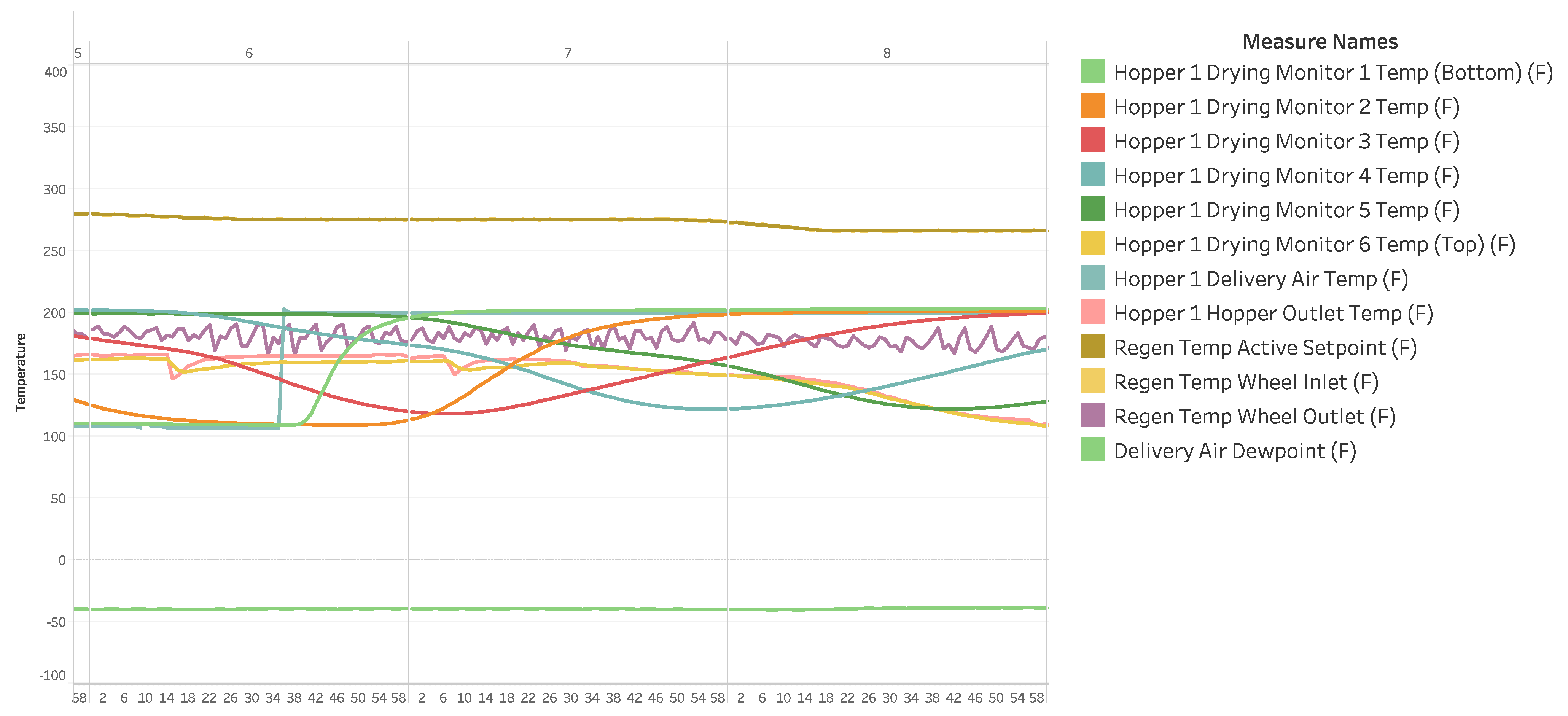
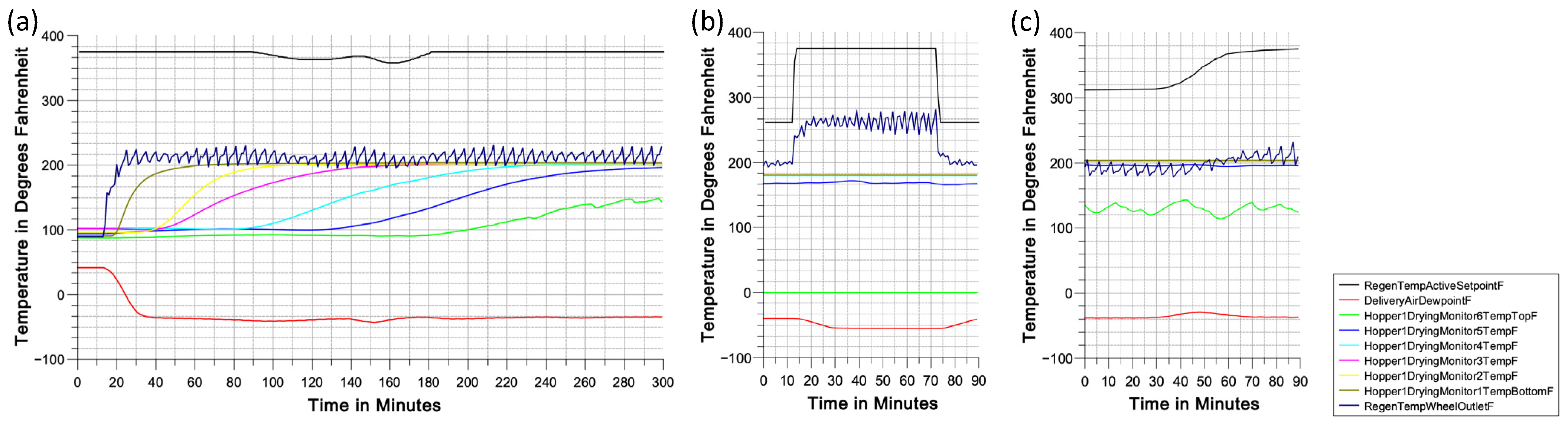
In this case study, three major events that occur regularly and affect operations have been identified: the startup procedure, cleaning cycle, and conveying issues [37]. These three events are shown as a snapshot of a visualization in the dataset in Figure 4. However, these events exhibit significant variation, making it difficult to define and label them precisely without having access to the domain expert. Moreover, having a limited number of samples in each event poses difficulty for a multiclass classification. Therefore, the primary objective of this study is to categorize events as either failures (unusual events) or regular events, rather than specifically detecting and classifying different types of unusual events. Unusual events are identified, selected, and labeled as one class, while the remaining events that represent the steady state are classified separately. If this approach proves successful, the subsequent goal is to identify the class of any labeled unusual event (beyond the steady state). This would enable valuable applications, such as providing context for process planners and operators, predicting necessary maintenance steps, and informing the design of future systems.

Two approaches can be used to label the data, focusing on either one main event or multiple major events: manual labeling and semi-supervised learning. Manual labeling requires significant time and effort from an expert who has a deep understanding of the process, making it a costly and time-consuming task, especially for datasets spanning a long period. Although manual labeling provides accurate labels, it may not be feasible for large datasets. The semi-supervised learning approach, on the other hand, requires only a small amount of labeled data, which are then used to predict the classes of the remaining unlabeled dataset. This enables the labeling of the entire dataset, which can be further trained to identify classes in the test set or future datasets. In this case study, manual labeling by a subject matter expert is performed to obtain the final labeled dataset. The labeling process aims to convert the dataset into a binary classification format, where steady state or regular events are treated as one class, and any unusual patterns or behaviors are treated as the other class. During labeling, we consider the whole one-hour window as an event if any major event happens anytime during that time window.

To label the time-series data, the original event duration data files are required. A sample rate of 60,000 is used to convert the time durations from the event duration dataset into milliseconds. An iterable variable is created with the time column of the original data. Using this variable and the event markings data, a column of 1 s and 0 s is generated to match the rows of the original dataset, indicating whether each minute is part of an event or non-event. However, labeling a minute of data may not accurately define an event, so instead, one hour of data consisting of sixty minutes or sixty rows is considered as an example. Each hour of data is treated as a subsequence, and subsequences are extracted from the long sequence of data with a specific length of sixty minutes (e.g., from 5:01:00 AM to 6:00:00 AM).

The labeling process involves assigning labels to each sixty-minute subsequence extracted from the time-series data. The sliding window algorithm is used to extract these subsequences, where a window length and sliding step need to be defined. In this case, the window length is set to sixty minutes, and the sliding step is also set to sixty minutes. The primary labeling assigns the same label to all sixty rows or minutes within each hour. After extracting the subsequences, the label for each hour is determined based on the labels assigned to all sixty rows or minutes within that hour. The sliding window algorithm is a common technique used for extracting subsequences from a longer time series, allowing for the extraction and labeling of multiple subsequences of a sixty-minute length [34]. In our case, the length of the time series, n, is 264,960; the window length, L, is 60; and the sliding step, p, is 60. So, m = (264,960 − 60)/60 + 1 = 4416. Hence, using a window length of sixty and sliding step of sixty, 4416 subsequences can be extracted from this time-series data.

After labeling each subsequence, the dataset can be viewed as a three-dimensional dataset with dimension N*L*M, where N represents the number of examples or subsequence, L represents the window or time-series length, and M represents the number of sensors or input variables of the MTS. Each subsequence has a dimension of L*M. In this case, L = 60 and M = 12, so, each subsequence has 60×12 = 720 features of the MTS. A basic summary of the labeled dataset is provided in

Table 1. The dataset statistics after preprocessing and labeling.

Dataset Statistics		Variable Types
Number of Variables	13	Numeric	12
Number of Observations	264,960	Categorical	1
Missing Cells (%)	0%
Duplicate Rows (%)	0.5%
Total size in memory	26.3 MiB

.

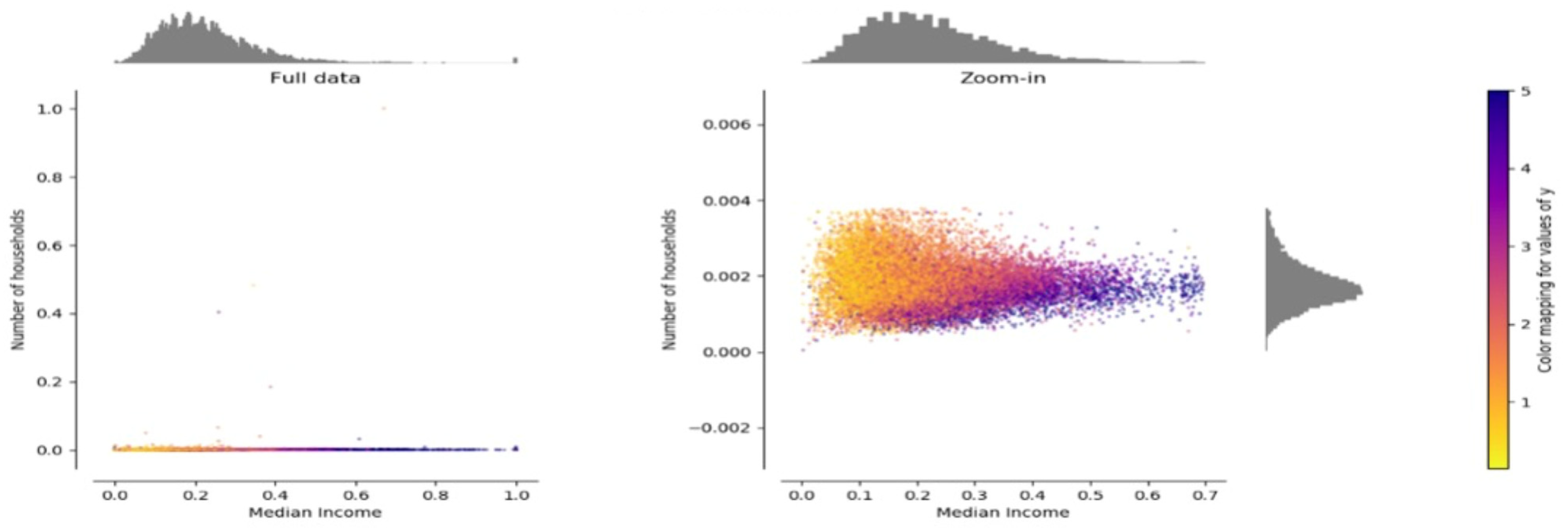
Data normalization, specifically via scaler transformation techniques, is highly recommended for machine learning and deep learning algorithms when dealing with skewed datasets. Skewed datasets can lead to imbalanced weights and distance measures between examples, affecting the performance of models such as SVM and K-nearest neighbor. For instance, in the given dataset, the delivery air temperature differs significantly from other temperatures in the drying hopper. By applying data normalization, the input variables are transformed to a standardized range, such as 0 to 1, making the learning process easier for algorithms, especially deep learning algorithms. Scaling helps avoid issues like high error gradient values and uncontrollable weight updates. Overall, pre-processing transformations, like data normalization, improve the performance and stability of models during learning [63]. Data normalization changes the distribution of the input variables, as shown in Figure 5.

3.1.3. Addressing the Imbalance Dataset Issue

The dataset used in this study faces the challenge of imbalanced classification, in which one class has significantly fewer examples than the other. Imbalanced datasets are common in real-world scenarios, especially in manufacturing, where failure events are rare compared to normal operations. While imbalanced datasets are very common in manufacturing settings and in fault detection problems, it is crucial to deal with the issue as a preprocessing step before fitting any ML algorithm to the dataset. DL algorithms are more sensitive in this sense and struggle more with imbalanced data due to their assumption of balanced datasets. To address this issue, the study explores four techniques: undersampling, oversampling, SMOTE, and ensemble learning with undersampling.

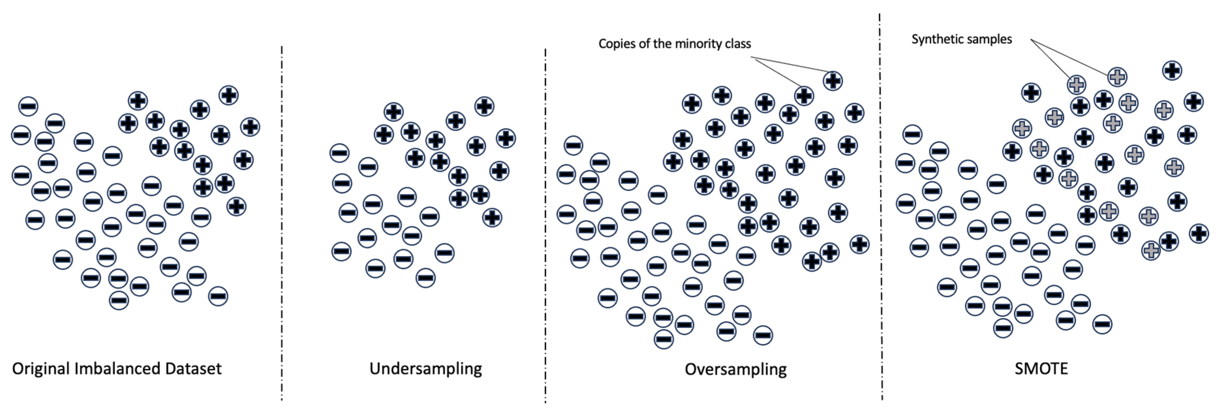
The simplest technique to address the imbalanced data issue is random undersampling, where a portion of the majority class data is dropped to achieve a balanced dataset for binary classification. In our case study, there are 845 examples in the minority class and 3571 examples in the majority class. The dataset is divided into training and test sets, with the first 80% of the data used for training and the remaining portion for testing. After the split, there were 791 training examples from the minority class and 2742 training examples from the majority class. Randomly selecting 791 examples from the majority class, a total of 1582 examples are used for training with a classification algorithm. The number of test examples after the split is 883, which are used to evaluate the algorithm. However, random undersampling can result in the loss of valuable information without considering the importance of the removed examples in determining the decision boundary between the classes [65].

Oversampling is another technique that can be utilized to deal with imbalanced datasets. The simplest oversampling technique involves duplicating the minority class randomly until it is equal in size to the majority class, thus achieving a balanced dataset. In our case, 791 training examples from the minority class are duplicated randomly to create 2742 examples, which are then added to the training dataset. This technique increases the number of training examples from 3533 to 5484. However, random oversampling can lead to overfitting, and the duplicated examples may not provide meaningful information to the dataset [66].

A more sophisticated approach called the Synthetic Minority Oversampling Technique (SMOTE) can be used, which synthesizes new data points based on existing examples [66]. SMOTE is a method that synthesizes new examples for the minority class. The technique, originally described in [67], is based on selecting examples that are nearest in the feature space. It creates a synthetic example by randomly selecting a neighbor from the K-nearest neighbors of a minority class example [68]. A line is then drawn in the feature space to connect the minority example and the selected neighbor. The synthetic examples are generated as a convex combination of the minority example and its nearest neighbors. SMOTE can produce as many synthetic examples as needed to achieve a balanced dataset. In this study, SMOTE will be used to oversample the minority class and balance the class distribution. The advantage of SMOTE over random oversampling is that the synthetic examples it generates are more reasonable and closer to the minority examples in the feature space. However, SMOTE has some drawbacks, such as not considering the majority class, which can lead to the creation of ambiguous examples that may not accurately represent the dataset. The visuals of undersampling, oversampling, and SMOTE techniques are shown in Figure 6.

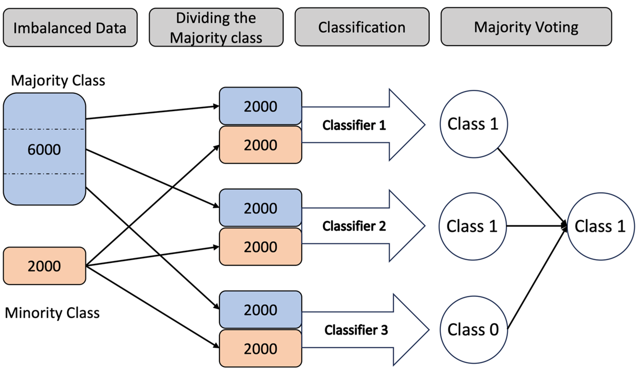
Ensemble learning is a powerful technique that can be used to deal with imbalanced data. Ensemble learning combines the results of multiple learning techniques to improve overall performance. In the context of dealing with imbalanced data, ensemble learning with undersampling can be employed. This involves dividing the majority class into segments and combining each segment with the minority class to train the dataset. An example of this approach is illustrated in Figure 7, where 3000 majority-class examples are divided into three segments, each containing 1000 randomly selected examples. These three sets of data, along with the entire minority class, are then used to train three classifiers. During testing, each classifier predicts the class for a given example, and the class with the majority vote is chosen as the ensemble prediction. In this study, three different approaches to ensemble learning are explored and their results are presented. By leveraging the collective knowledge of multiple classifiers, ensemble learning aims to enhance classification performance and address the challenges posed by imbalanced datasets [69].

3.2. Selection and Application of DL Networks

The following DL network architectures are used in this work: CNN network, LSTM network, and a combination of CNN and LSTM networks. The three variants are illustrated in Figure 8, Figure 9 and Figure 10, respectively. CNNs have gained widespread popularity due to their significant contributions to computer vision tasks. They have been extensively used in image recognition, natural language processing, and speech recognition. While initially developed for computer vision, CNNs have become one of the most popular deep neural networks for tackling time-series problems, particularly MTS problems. In time-series applications, 1D filters are used on subsequences of the long time series to perform dimensionality reduction. The CNN network in this study consists of two 1D-convolution layers, each followed by a dropout layer and a pooling layer at the end. The output is then connected to a fully connected dense layer and a single output neuron with a sigmoid activation function to perform the binary classification.

LSTM is a special type of RNN with gated cells that control the flow of information, allowing it to retain important long-term information while discarding irrelevant short-term information. This addresses the problem of exploding and vanishing gradients. LSTM uses a repeating chain-like structure with interacting layers in each unit. The LSTM network in this study comprises an individual hidden layer of LSTM with a dropout layer, followed by a common fully connected feedforward layer and a single output neuron with a sigmoid activation function to perform the binary classification.

The CNN-LSTM, a combination of CNN and LSTM, is effective for capturing internal features in sequential data like time series or image sequences. This architecture, which may also include an MLP, is suitable for datasets with both 2D and 1D structures, where the input or output exhibits temporal characteristics. For instance, the drying hopper temperature profile contains spatial features like peak temperature values and specific patterns, along with temporal dependencies, making the CNN-LSTM network a logical choice for processing such data. The CNN-LSTM architecture in this study employs 1D-CNN layers in the feature extraction process of input data incorporated with LSTMs to support sequence forecasting, as shown in Figure 10.

In this paper, in addition to the mentioned deep learning algorithms, several machine learning algorithms are used along with deep learning techniques to perform a comprehensive evaluation of these algorithms on the drying hopper use case dataset. Both non-linear algorithms like K-nearest neighbors, classification, and regression tree, SVM, and naïve Bayes, as well as ensemble algorithms like bagged decision trees, random forest, extra trees, and gradient boosting, are used to evaluate the performances of these algorithms compared to the deep learning algorithms and traditional methods like dynamic time warping with K-nearest neighbor.

3.3. Performance Metrics

In this study, accuracy, precision, recall, and f1 scores with the below definitions are used as performance measures. To calculate these measures, four terms need to be introduced, which are True Positive (TP), True Negative (TN), False Positive (FP), and False Negative (FN). For the rest of this paper, non-events are identified as the positive class, whereas events are identified as the negative class, where FP refers to the events wrongly identified as non-events, TN refers to the events accurately identified as events, FN refers to the non-events wrongly identified as events, and TP refers to non-events accurately identified as non-events. Accuracy is defined as the ratio between correctly classified examples and the total number of examples. It can be misleading, especially in the case of an imbalanced dataset. Precision is defined as the ratio between correctly predicted positive class and all predicted positive class examples, or the definition can be provided in terms of negative class as well. It is a common measure to identify the percentage of examples from a class that are correctly identified in terms of predicted labels. Recall is defined as the ratio between the examples that are actually positive and the examples that are predicted as negative, but actually positive. This definition can be extended to the negative class perspective as well. It is also a measure to identify the percentage of examples from a class that are correctly identified in terms of the actual labels. The F1 score is probably the most suitable performance measure that considers the data imbalance issue. It is a more structured performance measure using precision and recall.

$$Accuracy=\frac{TP+TN}{TP+TN+FP+FN}$$

(1)

$$Precision=\frac{TP}{TP+FP}$$

(2)

$$Recall=\frac{TP}{TP+FN}$$

(3)

$$F1=\frac{2\times Precision\times Recall}{Precision+Recall}$$

(4)

4. Results

In this chapter, the experimental setup is described and the results are shown. Furthermore, a comparative analysis was performed on the deep learning algorithms and traditional techniques dedicated to time series.

4.1. Experimental Setup

In this paper, the Python programming language was used for data preprocessing, model development, experimental runs, and evaluation. A variety of Python frameworks like Pandas and Numpy for data preprocessing and neural network frameworks like Tensorflow and Keras were used for model development and experimentation. The experiment was run on Windows 10, Intel^® core TM i5-3337U CPU @ 1.8 GHz.

The dataset in this study suffered from class imbalance, with only 22.39% of examples belonging to class 1. The distribution of different classes in the dataset is in

Table 2. Training and test set in the case study dataset.

Dataset	Class	No. of Examples	Percentage
Training Set	Event (class 1)	791	22.39%
	Non-event (class 0)	2742	77.61%
Test Set	Event (class 1)	50	5.66%
	Non-event (class 0)	833	94.34%

. When deep learning models such as CNN, LSTM, and MLP were trained on the imbalanced data, the test accuracy was misleadingly high at 94.34%, primarily due to the majority class overwhelming the predictions. To address this issue, three techniques were employed: ensemble learning, oversampling, and SMOTE. In ensemble learning, the training dataset was divided into groups, and multiple models were trained on each group. Majority voting was used to combine the predictions. Three different approaches were taken for ensemble learning, each with different groupings of the data.

Approach 1: The 2742 training examples of class 0 were divided into five groups. The first three groups had 548 examples each, the other two groups had 549 examples each. Then, 548 or 549 examples from class 1 were chosen randomly. These 548 examples from class 1 and class 0 were combined and shuffled to obtain one group of datasets for training. In this way, five groups of training sets were generated; each of them was trained using a separate model, and majority voting was used.

Approach 2: The 2742 training examples of class 0 were divided into three groups. The first two groups had 791 examples each and the last group had 1160 examples. Afterward, 791 examples of class 1 were combined with each group to build three groups of datasets. Each group was shuffled properly before training. In this way, three groups of training sets were generated; each of them was trained under a separate model using majority voting.

Approach 3: The 2742 training examples were divided into three equal segments where each of the groups had 914 examples. Afterward, 791 examples were combined and shuffled with each of the three groups. This way, each training dataset had 1705 training examples. Majority voting was used similarly.

For oversampling, examples from the minority class were randomly chosen and combined with the majority class to balance the data. SMOTE, a synthetic oversampling technique, was also utilized. The effectiveness of these techniques was evaluated in terms of precision and recall.

4.2. Hyperparameter Tuning

To use deep learning algorithms, hyperparameter tuning was a very important step. A lot of hyperparameters exist in a deep learning algorithm from which the ideal combination needs to be selected for optimal performance.

Table 3. Parameter and hyperparameter used for DL model training. # symbol indicate the number.

Model/Layer	Hyperparameter	Values
CNN	# Filters	8, 16
	Filter Size	3, 5, 7
	Activation Function	ReLu
LSTM	No. of LSTM neurons	100
Dropout	Dropout rate	0.5
Max Pooling	Pooling Size	2
Fully connected Layer	Dense Activation Function	ReLu
	Output Activation Function	Sigmoid
	No. of Neurons	200
Model Parameters	Batch Size	32, 64, 128
	Learning Rate	0.01
	No. of Epochs	100

shows the summary of the hyperparameters and model parameters for the initial experiment on hyperparameter tuning.

A series of experiments were conducted to determine the optimal hyperparameters for the neural network model. Different values for the number of filters, filter size, and batch size were tested, whereas other hyperparameters were kept constant. Ten experimental runs were performed to assess the test accuracy and variability for each set of hyperparameters. Box plots shown in Figure 11 were generated to visualize the results, showing that filter size 5 exhibited less variability in accuracy compared to other sizes.

The number of filters was selected as 16 due to its higher average accuracy, and a batch size of 64 was chosen for its higher average and lower variability. These finalized hyperparameters, along with other constant values, were used in a final test run. A validation split of 10% was employed, and the graph of accuracy and loss over epochs, as shown in Figure 12, indicated convergence to an optimal solution. However, since overfitting was observed, as evidenced by the fluctuating learning curve, the number of epochs was set to 10 for the final experiment.

4.3. Experiment Results

We followed the approach proposed in [22] and, in the final experiment, 10 runs were conducted for each deep learning and machine learning algorithm. The primary objective in this drying hopper case was to accurately detect events for predictive maintenance purposes. Since the number of non-events was significantly higher, correctly identifying non-events automatically resulted in high accuracy regardless of whether the model was able to identify the events or not. However, the precision of class 0 (non-events) and recall of class 1 (events) were crucial in this case, as they indicated the number of FPs. It is desirable to have the precision of class 0 and recall of class 1 as high as possible or the number of FPs as low as possible.

The summary of the ten experimental runs using CNN on the dataset using the ensemble learning approach for dealing with imbalancedness is presented in

Table 4. Result summary of CNN using different ensemble learning approaches.

Ensemble	Metrics	Best Experimental Run	Average Accuracy of 10 Runs
Approach 1	TP	832	0.9866
	TN	49
	FP	1
	FN	1
	Accuracy	0.9977
Approach 2	TP	833	0.9900
	TN	48
	FP	2
	FN	0
	Accuracy	0.9977
Approach 3	TP	833	0.9930
	TN	49
	FP	1
	FN	0
	Accuracy	0.9989

. Among the three approaches, Approach 3 achieved the best average accuracy of 99.30%. The FP values (events identified as non-events) ranged from 1 to 2, while the FN values (non-events identified as events) varied between 0 and 7 in the ten experimental runs. The first experimental run in approach 3 performed the best, misclassifying only one example as a non-event, which was an event. The table depicts the best results obtained from these three approaches in the ten experimental runs.

In the experimental setup, ensemble learning was applied by combining undersampling approaches and using majority voting to predict the class of test examples. Among the three approaches, Segment 2 of Approach 3, which combined 914 training examples of class 0 and 791 training examples of class 1, achieved the best results in four experimental runs. This indicates that these 914 training examples of class 0 contained significant information for training a CNN model. By using CNN and ensemble learning, the number of FPs can be reduced to 1 and FNs to 0. The best accuracy achieved using CNN and ensemble learning was 99.30% (Approach 3), with only one example being misclassified in the maximum number of runs. The results are presented in

Table 5. Best undersamples in 10 experimental runs using CNN network.

Metrics	Run 1	Run 2	Run 3	Run 4	Run 5	Run 6	Run 7	Run8	Run 9	Run 10
TP	833	833	833	831	833	833	833	831	833	833
TN	49	49	47	49	48	49	49	49	49	48
FP	1	1	3	1	2	1	1	1	1	2
FN	0	0	0	2	0	0	0	2	0	0
Accuracy	0.9989	0.9989	0.9966	0.9966	0.9977	0.9989	0.9966	0.9966	0.9989	0.9977
Approach and Segment	App 3, Seg 2	App 3, Seg 2	App 1, Seg 4	App 2, Seg 3	App 2, Seg 2	App 3, Seg 2	App 3, Seg 2	App 2, Seg 2	App 1, Seg 2	App 1, Seg 2

.

The hyperparameter setup for LSTM was the same as that of CNN, including the fully connected layer. The experiment began with 200 LSTM units in the LSTM layer following the input layer, and significant results were obtained. The summary of the ten experimental runs using the LSTM network on the dataset using the ensemble learning approach for dealing with imbalancedness is presented in

Table 6. Result summary of LSTM network using different ensemble learning approaches.

Ensemble	Metrics	Best Experimental Run	Average Accuracy of 10 Runs
Approach 1	TP	833	0.9874
	TN	48
	FP	2
	FN	0
	Accuracy	0.9977
Approach 2	TP	832	0.9855
	TN	48
	FP	2
	FN	1
	Accuracy	0.9966
Approach 3	TP	831	0.9905
	TN	48
	FP	2
	FN	2
	Accuracy	0.9955

. In the case of LSTM, Approach 3 demonstrated the best result. The results were quite similar to CNN, with the three approaches producing almost identical outcomes with slight variations. Approach 3 once again delivered the best average accuracy. The subsequent table displays the best results achieved in the ten experimental runs for LSTM.

Table 7. Best undersamples in 10 experimental runs using LSTM network.

Metrics	Run 1	Run 2	Run 3	Run 4	Run 5	Run6	Run 7	Run 8	Run 9	Run 10
TP	833	831	832	832	833	827	833	833	828	831
TN	47	49	47	48	47	48	48	48	49	49
FP	3	1	3	2	3	2	2	2	1	1
FN	0	2	1	1	0	6	0	0	5	2
Accuracy	0.9966	0.9966	0.9955	0.9966	0.9966	0.9909	0.9977	0.9977	0.9932	0.9966
Approach and Segment	App 2, Seg 3	App 2, Seg 3	App 1, Seg 3	App 3, Seg 2	App 2, Seg 2	App 1, Seg 3	App 1, Seg 2	App 1, Seg 2&3	App 2, Seg 3	App 2, Seg 3

displays the best undersamples of the ensemble learning in each run for LSTM. In four experimental runs, the best result was obtained from Segment 2 of Approach 1, where 1160 training examples of class 0 (1583 to 2742) and 791 training examples of class 1 were combined. This indicates that these 1160 training examples of class 0 are valuable for training an LSTM model. Thus, by using LSTM and ensemble learning, the number of FPs can be reduced to 2 and FNs to 0. The highest accuracy obtained using LSTM and ensemble learning was 99.05% (approach 3), where two examples were misclassified in most runs.

The same hyperparameters setup used in CNN and LSTM was used for the CNN-LSTM model. The summary of the ten experimental runs using the CNN-LSTM network on the dataset using the ensemble learning approach for dealing with imbalancedness is presented in

Table 8. Result summary of CNN-LSTM network using different ensemble learning approaches.

Ensemble	Metrics	Best Experimental Run	Average Accuracy of 10 Runs
Approach 1	TP	833	0.9875
	TN	48
	FP	2
	FN	0
	Accuracy	0.9977
Approach 2	TP	833	0.9826
	TN	48
	FP	2
	FN	0
	Accuracy	0.9977
Approach 3	TP	833	0.9807
	TN	47
	FP	3
	FN	0
	Accuracy	0.9966

. Although Approach 3 worked best for the CNN and LSTM models, for CNN-LSTM, Approach 1 worked well with 98.75% average accuracy across ten runs.

The best undersamples of the ensemble learning in each run are shown in

Table 9. Best undersamples in 10 experimental runs using CNN-LSTM network.

Metrics	Run 1	Run 2	Run 3	Run 4	Run 5	Run 6	Run 7	Run 8	Run 9	Run 10
TP	833	832	832	833	833	832	832	832	833	831
TN	49	48	48	48	48	47	48	46	46	49
FP	1	2	2	2	2	3	2	4	4	1
FN	0	1	1	0	0	1	1	1	0	2
Accuracy	0.9989	0.9966	0.9966	0.9977	0.9977	0.9955	0.9966	0.9943	0.9955	0.9966
Approach and Segment	App 2, Seg 2	App 1, Seg 4	App 1, Seg 3	App 1, Seg 2	App 3, Seg 2	App 2, Seg 3	App 3, Seg 2	App 2, Seg 2	App 2, Seg 3	App 1, Seg 5

. By using a combination of CNN and LSTM, we can reduce the number of FPs to as low as 1 and FNs to 0. Although Approach 1 worked best in terms of average accuracy, it had some outliers across ten runs, which was not the case for Approaches 2 and 3.

Table 10. Result summary of using SMOTE as the oversampling technique using different networks.

Network	Metrics	Best Experimental Run	Average Accuracy of 10 Runs
CNN	TP	833	0.9942
	TN	49
	FP	1
	FN	0
	Accuracy	0.9989
LSTM	TP	832	0.9830
	TN	49
	FP	1
	FN	1
	Accuracy	0.9977
CNN-LSTM	TP	832	0.9900
	TN	49
	FP	1
	FN	1
	Accuracy	0.9977

shows the summary of the ten experimental runs using SMOTE to deal with imbalancedness. In the training set, 2742 examples belonged to class 0, and 791 examples belonged to class 0. Using SMOTE, 1951 more samples were generated from the minority class, so class 1 also had 2742 examples. These 5484 examples were combined and shuffled properly for training the dataset using CNN, LSTM, and CNN-LSTM.

Overall, CNN performed very well when SMOTE was used for data augmentation, achieving an average accuracy of 99.42% across ten runs with no outliers in FP values. By utilizing SMOTE, CNN demonstrated outstanding performance, reducing the number of FP to 1 and FN to 0. Additionally, CNN exhibited less variability in terms of FP and FN values, with only one outlier in FNs.

To compare the performance of deep learning with other existing approaches, some machine learning algorithms were used like K-nearest neighbor (KNN), Support Vector Machine (SVM), Naïve Bayes (NB), Decision Tree (DT), Random Forest (RF), and Gradient Boosting (GB).

Table 11. Result summary of applying machine learning algorithms on the original dataset and augmented dataset using SMOTE.

Network	Metrics	KNN	SVM	NB	DT	RF	GB	Best Algorithm
Original Dataset	TP	833	822	817	813	820	822	SVM & GB
	TN	38	49	48	50	49	49
	FP	12	1	2	0	1	1
	FN	0	11	16	20	13	11
	Accuracy	0.9864	0.9864	0.9796	0.9773	0.9841	0.9864
	Run Number	3	1	4	9	2	3
	Average Accuracy	0.9742	0.9789	0.9692	0.9621	0.9735	0.9684	SVM
Augmented Dataset with SMOTE	TP	833	818	817	815	815	820	GB
	TN	44	50	48	49	49	49
	FP	6	0	2	1	1	1
	FN	0	15	16	18	18	13
	Accuracy	0.9932	0.9830	0.9796	0.9785	0.9785	0.9841
	Run Number	6	2	5	1	8	6
	Accuracy	0.9813	0.9766	0.9703	0.9643	0.9601	0.9732	KNN

summarizes the results obtained from the machine learning model using the original, non-augmented dataset, and the SMOTE dataset.

5. Discussion

The results across all evaluated algorithms using different approaches shown in the previous section are summarized below. It shows the average result obtained (accuracy) for an algorithm in ten experimental runs.

Table 12. Result summary (average result in ten runs).

Method	Ensemble Learning
	Approach 1			Approach 2			Approach 3
Algorithm	CNN	LSTM	CNN-LSTM	CNN	LSTM	CNN-LSTM	CNN	LSTM	CNN-LSTM
Accuracy	0.9866	0.9874	0.9875	0.9900	0.9855	0.9826	0.9930	0.9905	0.9807
Method		SMOTE
	Approach 1			Approach 2			Approach 3
Algorithm	CNN	LSTM	CNN-LSTM	KNN	SVM	NB	DT	RF	GB
Accuracy	0.9942	0.9830	0.9900	0.9813	0.9766	0.9703	0.9643	0.9601	0.9732

and

Table 13. Result summary (average result in ten runs).

Method	Original Dataset
Algorithm	KNN	SVM	NB	DT	RF	GB
Accuracy	0.9742	0.9789	0.9692	0.9621	0.9735	0.9684

summarize the results. From this summary, it is evident that the CNN method works best in terms of average results in ten experimental runs for this problem. For ensemble learning, Approach 3 shows the best accuracy using CNN, and for SMOTE, CNN works best among all algorithms.

In the following subsections, we discuss some of the challenges we faced in this study, the applied solutions, and the lessons learned.

5.1. Event Definition and Subsequence Extraction

The purpose of this study was to automatically detect unusual events in an industrial drying hopper in the polymer manufacturing industry. The raw dataset obtained from the machine interface required preprocessing from an expert to be suitable for ML or DL algorithms. Despite primary preprocessing, the dataset still had missing values and lacked labeling. The challenge was to define accurate unusual events based on temperature profiles, as there was no clear classification of different classes. To address this, events were defined at the beginning of the experiment, considering all variations in unusual events. Some assumptions were made to maintain consistency in defining events, such as disregarding certain small peaks in temperature values lasting only a few minutes. Two major limitations were the lack of a physics-based model for the drying hopper and the wide variety of potential event variations.

The study aimed to identify any unusual event rather than specifying the type of event. An hourly basis was used to simplify labeling, where each hour with unusual temperature profiles was labeled as an event. A sliding window approach was employed in the data preprocessing step, with a window length and sliding step of 60 min, resulting in 4416 examples. Alternative sliding step values could have been used, but this would complicate the labeling process, as not all rows would have the same labels. Defining events based on a percentage of rows labeled as 1 in an hour might lead to misinterpretations.

5.2. Data Imbalance Issue

During the training phase, the dataset showed class imbalance, with 77.61% examples from class 0 and 22.39% from class 1. The initial trial using a simple neural network misclassified all test examples as class 0. This issue was classified as an imbalance classification problem. Subsequent attempts using CNN, LSTM, and CNN-LSTM on the imbalanced dataset resulted in the same misclassification as the simple neural network. However, SVM, KNN, and other machine learning algorithms performed well with the imbalanced dataset.

To address the imbalance issue for deep learning algorithms, ensemble learning with undersampling, and SMOTE as an oversampling technique were employed, leading to reasonable results. For machine learning algorithms, SMOTE was also used as a data augmentation technique to assess their performance. Undersampling models were combined as an ensemble learner, as using a single undersampling approach alone might not guarantee optimal performance. Ensemble learning with majority voting resolved issues where some undersamples performed poorly due to the stochastic nature of the deep learning algorithms. Random oversampling was not utilized due to its lack of value and potential overfitting. However, SMOTE being a more structured oversampling approach, was preferred to control overfitting effectively using techniques like L2 regularization and dropout.

Additionally, class weighting was tested by assigning higher weights to the minority class during training. However, this approach did not yield satisfactory results, as all test examples were still classified as the majority class. As a result, the thesis focused solely on ensemble learning with undersampling and SMOTE as oversampling techniques to address the data imbalance problem.

5.3. Result Interpretation

In this study, the performance measures used are precision, recall, F1 score, and accuracy. Precision, recall, and accuracy depend on TP, TN, FP, and FN values, whereas the F1 score is derived from precision and recall. In the context of manufacturing, fault detection is crucial for predictive or preventive maintenance. The main goal is to accurately identify events to avoid machine failure or related issues. Minimizing FP values (events wrongly identified as non-events) and maximizing TN values (events accurately identified as events) are the primary objectives. Reducing FN values (non-events wrongly identified as events) and increasing TP values (non-events accurately identified as non-events) are the secondary objectives. For instance, if the algorithm identifies a non-event as an event, the operator needs to manually verify it, which could be time-consuming if such instances are frequent. On the other hand, if the algorithm identifies an event as a non-event, it can lead to serious issues as the operator remains unaware of the actual problem. In this case, the operator has two and a half hours to fix the identified event, given that each example’s length is one hour. Therefore, after training the dataset and performing primary preprocessing, the algorithm can predict the class of any future one-hour example extracted from sensors and take appropriate actions accordingly. With Industry 4.0 and the AI revolution, this type of automation is highly important in any manufacturing plant.

The primary goal in manufacturing is to reduce FP values. In the experimental setup, consistency in the number of FP values across ten runs is desirable for algorithms using ensemble learning or SMOTE. The objective of each run is to find the best model with high accuracy and fewer FP values. The selection process involves picking the model with the highest accuracy first, and if it also has fewer FP values, it is considered the best model. In most cases, the model with the best accuracy also has the least number of FP values, though there are some exceptions where the accuracy is high due to correctly identifying many non-events.

Overall, CNN performs exceptionally well in terms of accuracy and consistency in FP and FN values, making it the preferred algorithm for classifying this dataset into two categories.

6. Conclusions and Future Works

The recent evolution in Industry 4.0, artificial intelligence, and the Internet of Things (IoT) has increased data availability in various domains. This is why data analytics has become highly popular over the years with newer algorithms and techniques being developed regularly for continuous improvement. Among different types of data, time-series data have become highly available in various domains and various analyses on time series are frequently being performed by researchers. This study explores the classification of time-series data obtained from the temperature sensors in a polymer manufacturing industry’s drying hopper using deep learning algorithms. The dataset required preprocessing to be suitable for deep learning and machine learning algorithms. The classification task involved defining two categories and addressing the imbalance in the data using ensemble learning with undersampling and SMOTE as an oversampling technique. The results indicated that CNN performed the best in classifying this dataset. Previous research on the same dataset focused on understanding the drying hopper process and pattern recognition [37,39]. Future work includes defining events more precisely, categorizing events into different types, exploring variable windowing techniques, and considering more advanced deep learning approaches, such as residual networks, multi-channel CNNs, and GRU variants for improved classification, especially for multiclass scenarios.

There are several limitations that must be considered when interpreting the results of this paper. This paper was written under certain assumptions, timelines, and resource limitations, with a primary focus on providing a general model that emphasizes preprocessing and addressing imbalance issues. Given the lack of clear physics-based definitions for events and non-events, the paper adopted a data-driven modeling approach, using the simplest method for event classification. While the complete removal of subjectivity and biases is impossible and arguably not desirable, our intention is to maintain transparency by articulating the process and methodology used, enabling our audience to understand our biases, intent, understanding, and their influence on the content of this paper.

References

1. Mccormick, M.R.; Wuest, T. Challenges for Smart Manufacturing and Industry 4.0 Research in Academia: A Case Study; ResearchGate: Berlin, Germany, 2023. [Google Scholar] [CrossRef]
2. Oztemel, E.; Gursev, S. Literature review of Industry 4.0 and related technologies. J. Intell. Manuf. 2020, 31, 127–182. [Google Scholar] [CrossRef]
3. Hsu, C.-Y.; Liu, W.-C. Multiple time-series convolutional neural network for fault detection and diagnosis and empirical study in semiconductor manufacturing. J. Intell. Manuf. 2021, 32, 823–836. [Google Scholar] [CrossRef]
4. Jones, S.S.; Evans, R.S.; Allen, T.L.; Thomas, A.; Haug, P.J.; Welch, S.J.; Snow, G.L. A multivariate time series approach to modeling and forecasting demand in the emergency department. J. Biomed. Inform. 2009, 42, 123–139. [Google Scholar] [CrossRef]
5. Du, Z.; Lawrence, W.R.; Zhang, W.; Zhang, D.; Yu, S.; Hao, Y. Interactions between climate factors and air pollution on daily HFMD cases: A time series study in Guangdong, China. Sci. Total Environ. 2019, 656, 1358–1364. [Google Scholar] [CrossRef]
6. Perez-D’Arpino, C.; Shah, J.A. Fast target prediction of human reaching motion for cooperative human-robot manipulation tasks using time series classification. In Proceedings of the 2015 IEEE International Conference on Robotics and Automation (ICRA), Seattle, WA, USA, 26–30 May 2015; pp. 6175–6182. [Google Scholar] [CrossRef]
7. Farahani, M.A.; Vahid, A.; Goodwell, A.E. Evaluating Ecohydrological Model Sensitivity to Input Variability with an Information-Theory-Based Approach. Entropy 2022, 24, 994. [Google Scholar] [CrossRef]
8. Maknickienė, N.; Rutkauskas, A.V.; Maknickas, A. Investigation of financial market prediction by recurrent neural network. Innov. Technol. Sci. Bus. Educ. 2011, 2, 3–8. [Google Scholar]
9. Martín, L.; Zarzalejo, L.F.; Polo, J.; Navarro, A.; Marchante, R.; Cony, M. Prediction of global solar irradiance based on time series analysis: Application to solar thermal power plants energy production planning. Sol. Energy 2010, 84, 1772–1781. [Google Scholar] [CrossRef]
10. Farahani, M.A.; McCormick, M.R.; Gianinny, R.; Hudacheck, F.; Harik, R.; Liu, Z.; Wuest, T. Time-series pattern recognition in Smart Manufacturing Systems: A literature review and ontology. J. Manuf. Syst. 2023, 69, 208–241. [Google Scholar] [CrossRef]
11. Muth, J.F. Optimal Properties of Exponentially Weighted Forecasts. J. Am. Stat. Assoc. 1960, 55, 299–306. [Google Scholar] [CrossRef]
12. Bagnall, A.; Lines, J.; Bostrom, A.; Large, J.; Keogh, E. The great time series classification bake off: A review and experimental evaluation of recent algorithmic advances. Data Min. Knowl. Discov. 2017, 31, 606–660. [Google Scholar] [CrossRef]
13. Berndt, D.J.; Clifford, J. Using Dynamic Time Warping to Find Patterns in Time Series. In Proceedings of the 3rd International Conference on Knowledge Discovery and Data Mining, Seattle, WA, USA, 31 July–1 August 1994; pp. 359–370. [Google Scholar]
14. Box, G.E.; Jenkins, G.M.; Reinsel, G.C.; Ljung, G.M. Time Series Analysis: Forecasting and Control; John Wiley & Sons: Hoboken, NJ, USA, 2015. [Google Scholar]
15. He, G.; Li, Y.; Zhao, W. An uncertainty and density based active semi-supervised learning scheme for positive unlabeled multivariate time series classification. Knowl.-Based Syst. 2017, 124, 80–92. [Google Scholar] [CrossRef]
16. Tuballa, M.L.; Abundo, M.L. A review of the development of Smart Grid technologies. Renew. Sustain. Energy Rev. 2016, 59, 710–725. [Google Scholar] [CrossRef]
17. Batal, I.; Sacchi, L.; Bellazzi, R.; Hauskrecht, M. Multivariate Time Series Classification with Temporal Abstractions. In Proceedings of the Twenty-Second International FLAIRS Conference, Sanibel Island, FL, USA, 19–21 May 2009. [Google Scholar]
18. Yang, K.; Shahabi, C. An efficient k nearest neighbor search for multivariate time series. Inf. Comput. 2007, 205, 65–98. [Google Scholar] [CrossRef]
19. Hills, J.; Lines, J.; Baranauskas, E.; Mapp, J.; Bagnall, A. Classification of time series by shapelet transformation. Data Min. Knowl. Discov. 2014, 28, 851–881. [Google Scholar] [CrossRef]
20. Chang, Y.; Rubin, J.; Boverman, G.; Vij, S.; Rahman, A.; Natarajan, A.; Parvaneh, S. A Multi-Task Imputation and Classification Neural Architecture for Early Prediction of Sepsis from Multivariate Clinical Time Series. In Proceedings of the 2019 Computing in Cardiology Conference, Singapore, 8–11 September 2019. [Google Scholar] [CrossRef]
21. Lines, J.; Bagnall, A. Time series classification with ensembles of elastic distance measures. Data Min. Knowl. Discov. 2015, 29, 565–592. [Google Scholar] [CrossRef]
22. Fawaz, H.I.; Forestier, G.; Weber, J.; Idoumghar, L.; Muller, P.-A. Deep learning for time series classification: A review. Data Min. Knowl. Discov. 2019, 33, 917–963. [Google Scholar] [CrossRef]
23. Krizhevsky, A.; Sutskever, I.; Hinton, G.E. ImageNet classification with deep convolutional neural networks. Commun. ACM 2017, 60, 84–90. [Google Scholar] [CrossRef]
24. Szegedy, C.; Liu, W.; Jia, Y.; Sermanet, P.; Reed, S.; Anguelov, D.; Erhan, E.; Vanhoucke, V.; Rabinovich, A. Going deeper with convolutions. In Proceedings of the 2015 IEEE Conference on Computer Vision and Pattern Recognition (CVPR), Boston, MA, USA, 7–12 June 2015; pp. 1–9. [Google Scholar] [CrossRef]
25. Bahdanau, D.; Cho, K.; Bengio, Y. Neural Machine Translation by Jointly Learning to Align and Translate. arXiv 2016, arXiv:1409.0473. [Google Scholar]
26. Sutskever, I.; Vinyals, O.; Le, Q.V. Sequence to Sequence Learning with Neural Networks. arXiv 2014, arXiv:1409.3215. [Google Scholar]
27. Alayba, A.M.; Palade, V.; England, M.; Iqbal, R. A Combined CNN and LSTM Model for Arabic Sentiment Analysis. In Machine Learning and Knowledge Extraction; Holzinger, A., Kieseberg, P., Tjoa, A.M., Weippl, E., Eds.; Lecture Notes in Computer Science; Springer International Publishing: Cham, Switzerland, 2018; Volume 11015, pp. 179–191. ISBN 978-3-319-99739-1. [Google Scholar]
28. Sainath, T.N.; Kingsbury, B.; Mohamed, A.; Dahl, G.E.; Saon, G.; Soltau, H.; Beran, T.; Aravkin, A.Y.; Ramabhadran, B. Improvements to Deep Convolutional Neural Networks for LVCSR. In Proceedings of the 2013 IEEE Workshop on Automatic Speech Recognition and Understanding, Olomouc, Czech Republic, 8–12 December 2013; pp. 315–320. [Google Scholar] [CrossRef]
29. Liu, C.-L.; Hsaio, W.-H.; Tu, Y.-C. Time Series Classification With Multivariate Convolutional Neural Network. IEEE Trans. Ind. Electron. 2019, 66, 4788–4797. [Google Scholar] [CrossRef]
30. Huang, H.-S.; Liu, C.-L.; Tseng, V.S. Multivariate Time Series Early Classification Using Multi-Domain Deep Neural Network. In Proceedings of the 2018 IEEE 5th International Conference on Data Science and Advanced Analytics (DSAA), Turin, Italy, 1–3 October 2018; pp. 90–98. [Google Scholar] [CrossRef]
31. Yazdanbakhsh, O.; Dick, S. Multivariate Time Series Classification using Dilated Convolutional Neural Network. arXiv 2019, arXiv:1905.01697. [Google Scholar]
32. Karim, F.; Majumdar, S.; Darabi, H.; Harford, S. Multivariate LSTM-FCNs for Time Series Classification. Neural Netw. 2019, 116, 237–245. [Google Scholar] [CrossRef] [PubMed]
33. Guo, Z.; Liu, P.; Yang, J.; Hu, Y. Multivariate Time Series Classification Based on MCNN-LSTMs Network. In Proceedings of the 2020 12th International Conference on Machine Learning and Computing, Shenzhen, China, 15–17 February 2020; pp. 510–517. [Google Scholar] [CrossRef]
34. Zheng, Y.; Liu, Q.; Chen, E.; Ge, Y.; Zhao, J.L. Exploiting multi-channels deep convolutional neural networks for multivariate time series classification. Front. Comput. Sci. 2016, 10, 96–112. [Google Scholar] [CrossRef]
35. Lei, K.-C.; Zhang, X.D. An approach on discretizing time series using recurrent neural network. In Proceedings of the 2018 IEEE International Conference on Bioinformatics and Biomedicine (BIBM), Madrid, Spain, 3–6 December 2018; pp. 2522–2526. [Google Scholar] [CrossRef]
36. Che, Z.; Purushotham, S.; Cho, K.; Sontag, D.; Liu, Y. Recurrent Neural Networks for Multivariate Time Series with Missing Values. Sci. Rep. 2018, 8, 6085. [Google Scholar] [CrossRef]
37. Lenz, J.; Swerdlow, S.; Landers, A.; Shaffer, R.; Geller, A.; Wuest, T. Smart Services for Polymer Processing Auxiliary Equipment: An Industrial Case Study. Smart Sustain. Manuf. Syst. 2020, 4, 20200032. [Google Scholar] [CrossRef]
38. Shokoohi-Yekta, M.; Wang, J.; Keogh, E. On the Non-Trivial Generalization of Dynamic Time Warping to the Multi-Dimensional Case. In Proceedings of the 2015 SIAM International Conference on Data Mining; Society for Industrial and Applied Mathematics, Vancouver, BC, Canada, 30 April–2 May 2015; pp. 289–297. [Google Scholar] [CrossRef]
39. Kapp, V.; May, M.C.; Lanza, G.; Wuest, T. Pattern Recognition in Multivariate Time Series: Towards an Automated Event Detection Method for Smart Manufacturing Systems. J. Manuf. Mater. Process. 2020, 4, 88. [Google Scholar] [CrossRef]
40. Shen, J.; Huang, W.; Zhu, D.; Liang, J. A Novel Similarity Measure Model for Multivariate Time Series Based on LMNN and DTW. Neural Process. Lett. 2017, 45, 925–937. [Google Scholar] [CrossRef]
41. Mei, J.; Liu, M.; Wang, Y.-F.; Gao, H. Learning a Mahalanobis Distance-Based Dynamic Time Warping Measure for Multivariate Time Series Classification. IEEE Trans. Cybern. 2016, 46, 1363–1374. [Google Scholar] [CrossRef]
42. Vaughan, N.; Gabrys, B. Scoring and assessment in medical VR training simulators with dynamic time series classification. Eng. Appl. Artif. Intell. 2020, 94, 103760. [Google Scholar] [CrossRef]
43. Ircio, J.; Lojo, A.; Mori, U.; Lozano, J.A. Mutual information based feature subset selection in multivariate time series classification. Pattern Recognit. 2020, 108, 107525. [Google Scholar] [CrossRef]
44. Górecki, T.; Łuczak, M. Multivariate time series classification with parametric derivative dynamic time warping. Expert Syst. Appl. 2015, 42, 2305–2312. [Google Scholar] [CrossRef]
45. Seto, S.; Zhang, W.; Zhou, Y. Multivariate Time Series Classification Using Dynamic Time Warping Template Selection for Human Activity Recognition. In Proceedings of the 2015 IEEE Symposium Series on Computational Intelligence, Cape Town, South Africa, 1–7 December 2015; pp. 1399–1406. [Google Scholar] [CrossRef]
46. Łuczak, M. Univariate and multivariate time series classification with parametric integral dynamic time warping. J. Intell. Fuzzy Syst. 2017, 33, 2403–2413. [Google Scholar] [CrossRef]
47. Baydogan, M.G.; Runger, G. Learning a symbolic representation for multivariate time series classification. Data Min. Knowl. Discov. 2015, 29, 400–422. [Google Scholar] [CrossRef]
48. Lin, J.; Keogh, E.; Wei, L.; Lonardi, S. Experiencing SAX: A novel symbolic representation of time series. Data Min. Knowl. Discov. 2007, 15, 107–144. [Google Scholar] [CrossRef]
49. Schäfer, P.; Högqvist, M. SFA: A symbolic fourier approximation and index for similarity search in high dimensional datasets. In Proceedings of the 15th International Conference on Extending Database Technology, Berlin, Germany, 27–30 March 2012; pp. 516–527. [Google Scholar] [CrossRef]
50. Le Nguyen, T.; Gsponer, S.; Ilie, I.; O’Reilly, M.; Ifrim, G. Interpretable time series classification using linear models and multi-resolution multi-domain symbolic representations. Data Min. Knowl. Discov. 2019, 33, 1183–1222. [Google Scholar] [CrossRef]
51. Dhariyal, B.; Le Nguyen, T.; Gsponer, S.; Ifrim, G. An Examination of the State-of-the-Art for Multivariate Time Series Classification. In Proceedings of the 2020 International Conference on Data Mining Workshops (ICDMW), Sorrento, Italy, 17–20 November 2020; pp. 243–250. [Google Scholar] [CrossRef]
52. Schäfer, P.; Leser, U. Multivariate Time Series Classification with WEASEL+MUSE 2018. arXiv 2018, arXiv:1711.11343. [Google Scholar]
53. 53. Zhao, B.; Lu, H.; Chen, S.; Liu, J.; Wu, D. Convolutional neural networks for time series classification. J. Syst. Eng. Electron. 2017, 28, 162–169. [Google Scholar] [CrossRef]
54. Ruiz, A.P.; Flynn, M.; Large, J.; Middlehurst, M.; Bagnall, A. The great multivariate time series classification bake off: A review and experimental evaluation of recent algorithmic advances. Data Min. Knowl. Discov. 2021, 35, 401–449. [Google Scholar] [CrossRef]
55. Song, W.; Liu, L.; Liu, M.; Wang, W.; Wang, X.; Song, Y. Representation Learning with Deconvolution for Multivariate Time Series Classification and Visualization. In Data Science; Zeng, J., Jing, W., Song, X., Lu, Z., Eds.; Springer: Singapore, 2020; Volume 1257, pp. 310–326. ISBN 9789811579806. [Google Scholar]
56. Kiangala, K.S.; Wang, Z. An Effective Predictive Maintenance Framework for Conveyor Motors Using Dual Time-Series Imaging and Convolutional Neural Network in an Industry 4.0 Environment. IEEE Access 2020, 8, 121033–121049. [Google Scholar] [CrossRef]
57. Martínez-Arellano, G.; Terrazas, G.; Ratchev, S. Tool wear classification using time series imaging and deep learning. Int. J. Adv. Manuf. Technol. 2019, 104, 3647–3662. [Google Scholar] [CrossRef]
58. Sainath, T.N.; Vinyals, O.; Senior, A.; Sak, H. Convolutional, Long Short-Term Memory, fully connected Deep Neural Networks. In Proceedings of the 2015 IEEE International Conference on Acoustics, Speech and Signal Processing (ICASSP), South Brisbane, QLD, Australia, 19–24 April 2015; pp. 4580–4584. [Google Scholar] [CrossRef]
59. Hsu, E.-Y.; Liu, C.-L.; Tseng, V.S. Multivariate Time Series Early Classification with Interpretability Using Deep Learning and Attention Mechanism. In Advances in Knowledge Discovery and Data Mining; Yang, Q., Zhou, Z.-H., Gong, Z., Zhang, M.-L., Huang, S.-J., Eds.; Lecture Notes in Computer Science; Springer International Publishing: Cham, Switzerland, 2019; Volume 11441, pp. 541–553. ISBN 978-3-030-16141-5. [Google Scholar]
60. Khan, M.; Wang, H.; Ngueilbaye, A.; Elfatyany, A. End-to-end multivariate time series classification via hybrid deep learning architectures. Pers. Ubiquitous Comput. 2023, 27, 177–191. [Google Scholar] [CrossRef]
61. Tripathi, A.M. Enhancing Multivariate Time Series Classification Using LSTM and Evidence Feed Forward HMM. In Proceedings of the 2020 International Joint Conference on Neural Networks (IJCNN), Glasgow, UK, 19–24 July 2020; pp. 1–7. [Google Scholar] [CrossRef]
62. Gruenwald, L.; Chok, H.; Aboukhamis, M. Using Data Mining to Estimate Missing Sensor Data. In Proceedings of the Seventh IEEE International Conference on Data Mining Workshops (ICDMW 2007), Omaha, NE, USA, 28–31 October 2007; pp. 207–212. [Google Scholar] [CrossRef]
63. Bishop, C.M. Neural Networks for Pattern Recognition; Clarendon Press: Oxford, UK; Oxford University Press: Oxford, NY, USA, 1995; ISBN 978-0-19-853849-3. [Google Scholar]
64. Pedregosa, F.; Varoquaux, G.; Gramfort, A.; Michel, V.; Thirion, B.; Grisel, O.; Blondel, M.; Prettenhofer, P.; Weiss, R.; Dubourg, V.; et al. Scikit-learn: Machine learning in Python. J. Mach. Learn. Res. 2011, 12, 2825–2830. [Google Scholar]
65. Ganganwar, V. An overview of classification algorithms for imbalanced datasets. Int. J. Emerg. Technol. Adv. Eng. 2012, 2, 42–47. [Google Scholar]
66. Zheng, Z. Oversampling Method for Imbalanced Classification. Comput. Inform. 2015, 34, 1017–1037. [Google Scholar]
67. Chawla, N.V.; Bowyer, K.W.; Hall, L.O.; Kegelmeyer, W.P. SMOTE: Synthetic Minority Over-sampling Technique. J. Artif. Intell. Res. 2002, 16, 321–357. [Google Scholar] [CrossRef]
68. He, H.; Ma, Y. Imbalanced Learning: Foundations, Algorithms, and Applications; John Wiley & Sons: Hoboken, NJ, USA, 2013. [Google Scholar]
69. Sun, Z.; Song, Q.; Zhu, X.; Sun, H.; Xu, B.; Zhou, Y. A novel ensemble method for classifying imbalanced data. Pattern Recognit. 2015, 48, 1623–1637. [Google Scholar] [CrossRef]
Figure 1. A view of a drying hopper with different temperature zones [39].
Jmmp 07 00164 g001
Figure 2. The temperature profile of the data gathered from the case study drying hopper.
Jmmp 07 00164 g002
Figure 3. Overview of the proposed MTS classification framework.
Jmmp 07 00164 g003
Figure 4. Three major events in case study operation. Startup procedure (a), cleaning cycle (b), and conveying issue (c) (adapted from [37]).
Jmmp 07 00164 g004
Figure 5. Change in distribution before normalization (left) and after normalization (right) (created based on [64]).
Jmmp 07 00164 g005
Figure 6. Different techniques to deal with imbalanced datasets.
Jmmp 07 00164 g006
Figure 7. Ensemble learning method [69].
Jmmp 07 00164 g007
Figure 8. The CNN network architecture.
Jmmp 07 00164 g008
Figure 9. The LSTM network architecture.
Jmmp 07 00164 g009
Figure 10. The CNN-LSTM network architecture.
Jmmp 07 00164 g010
Figure 11. Hyperparameter tuning results. # symbol indicates the number of filters.
Jmmp 07 00164 g011
Figure 12. Accuracy and loss vs. Epoch.
Jmmp 07 00164 g012