Article

Development of a Computationally Efficient Model of the Heating Phase in Thermoforming Process Based on the Experimental Radiation Pattern of Heaters

School of Engineering, University of British Columbia, Kelowna, BC V1V 1V7, Canada
*
Author to whom correspondence should be addressed.
J. Manuf. Mater. Process. 2023, 7(1), 48; https://doi.org/10.3390/jmmp7010048
Submission received: 9 January 2023 / Revised: 6 February 2023 / Accepted: 7 February 2023 / Published: 10 February 2023

Abstract

:
In this study, an accurate and computationally efficient model for the heating process of thin thermoplastic sheets during thermoforming is developed. This model opens the door to efficient training of model-free control approaches in thermoforming applications, which often require extensive training data that would be significantly costly and time-consuming to generate using physical setups. This model takes into account heat transfer via radiation between heaters and the sheet, heat transfer via conduction through the sheet, and heat transfer via convection between the sheet and the ambient. In this paper, rather than using an analytical relationship for the view factor, an experiment is designed to determine the exact radiation pattern of the heater on the sheet and the fraction of infrared emission absorbed by the sheet. Comparing the output temperature profile on the sheet from the designed model to IR images from a laboratory-scale heating system indicates that the mean square error is reduced by around four times when compared to traditional models with analytical view factors. Moreover, a comparison of the computation time with COMSOL software for a scenario with the same configuration of computation hardware reveals that the designed model is almost ten times faster.

1. Introduction

Composite manufacturing is a clear example of a process that has the potential to be impacted by industry 5.0 [1], due to the large number of manufacturing steps that are still performed manually or with minimal automation. Any controller design requires an accurate model that describes the system’s behavior. For traditional model-based control, it determines the controller structure and allows for optimizing the control system’s performance [2]. For model-free controllers, a precise model can be used to replace expensive physical experiments during the training phase of the control systems. Many studies have been conducted to reduce the infeasible requirement of large data availability for developing accurate learning models [3,4]. However, since model-free control methods such as Reinforcement Learning (RL) require a large number of “trial and error” episodes or interactions within an environment Figure 1, utilizing simulators is a cost-effective and time-efficient strategy for achieving results [5,6,7]. Once the algorithm has been sufficiently trained offline through interaction with a simulated environment, offline learning would stop, and the trained algorithm would be deployed on the target hardware, similar to a control law. At this stage, the need for continued training on target hardware is highly dependent on the accuracy of the simulator during the offline training.
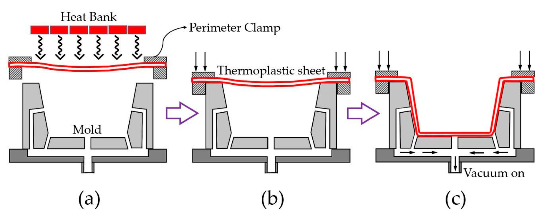
Moreover, a precise model is also necessary for simulating the developed control technique to ensure the stability and robustness of the proposed technique prior to its implementation in the real world. In this paper we present a refined 2D model for the heating phase of thermoforming processes that, for the first time, takes into account the geometry of the physical heating elements employed, and we will show that this can remarkably reduce modelling errors. Thermoforming is the process of heating and deforming a thermoplastic sheet into the desired shape [8,9]. The typical sequence of this process as described by Leite et al. [10] is presented in Figure 2. Typically, radiant heaters are positioned on one or both sides of the plastic sheet. The length of the heating cycle required to adequately soften the sheet depends on the physical, chemical, and mechanical properties of the polymer, its thickness, and its color.
Thickness non-uniformity and webs are common types of defects that can occur during the thermoforming process [10]. Traditionally, the thermoforming industry has relied on operators manually adjusting heating elements to minimize defects. Clearly, feedback control schemes could improve this approach, but they require an accurate and computationally efficient process model. Obtaining and creating an optimal temperature profile on the sheet for a particular mold in order to prevent defects in the final product is a crucial aspect of the thermoforming process. Thermoplastic sheet deformation models during the thermoforming process can be used in an optimization algorithm to achieve this optimal temperature profile. In these models, the temperature profile on the sheet impacts the physical and thermomechanical properties in different zones, resulting in different sheet thicknesses as a final product. Hosseini et al. [11] created a model that describes how a pre-stretched sheet deforms during any stage of the vacuum thermoforming process. Additionally, they developed a method based on the wall-thickness distribution criterion for predicting and improving the quality of the finished products. Wang et al. [12] presented a simulation method for multilayer thermoplastic deformation during thermoforming. Semi-discrete shell elements were used to model each prepreg layer. Xiong et al. [13] studied the consolidation behavior of thermoplastic composite prepregs during the thermoforming process based on a generalized Maxwell approach. Wang et al. [14] presented a fully coupled thermomechanical computational model based on the hot optimal transportation mesh-free method for resin-based friction composites. Wanger et al. [15] developed a model for thermoforming that includes, approximatively, the effects of the flow field within the pressure box on the plastic sheet that is deforming. Bean et al. [16] developed a tool that employs the local fiber alignment and thickness predictions from the forming simulation to generate a more precise structural model. It is anticipated that this will provide a more accurate prediction of the final part’s performance than a structural model that utilizes initial ply thicknesses and fiber orientations. Consequently, the utility of a forming simulation is increased.
The present paper focuses on the heating phase of the thermoforming process to develop a 2D model of heat transfer between the thermoplastic sheet, heating elements, and environment. To this end, a 2D finite differential analysis is combined with an energy balance method in order to model the heating process during the thermoforming of thin thermoplastic [17,18,19,20] sheets. This process is most often modelled using 1D, 2D, and 3D finite element methods [21], 1D and 2D finite difference methods [22], and 3D control-volume methods [23]. Duarte and Covas [24,25] investigated the inverse heating problem for thermoforming machines that use thin sheet materials. They created a model based on an analytical view factor to determine the optimal heating element temperatures that would result in a uniform sheet surface temperature. Monteix et al. [26] developed a method for determining radiant heat transfer within a plastic sheet using a control-volume method. They considered the specific heater geometry, taking into account a view factor computation. They assumed a constant filament temperature and a uniform source temperature to calculate the amount of incident radiation reaching each element of the sheet with the contour integration method. In a simulation, larger finite-element models of the thermoforming process are applied to predetermine the ideal operating parameters for exact sheet thickness distribution during thermoforming. Yousefi et al. [27] improved FEM modelling of the reheat phase in thermoforming by treating parameter uncertainty. They performed a series of experiments to identify the key parameters through sensitivity analysis. Gauthier et al. [28] proposed a number of enhancements to the heating phase of a thermoforming machine by taking into account the heat transmission coefficient over the plastic surface. He evaluated the portion of heat energy that is transmitted through the plastic sheet layer and the portion that is absorbed by the same plastic sheet using the Beer-Lambert Law. Chy et al. [29] improved Gauthier‘s model by means of a more accurate evaluation of input parameters for convection heat transfer, investigation of other heating sources, and the development of a model for the air temperature inside the oven. Erchiqui (in [30]) considered a specific 3D volumetric enthalpy-based finite element method. They also used a technique based on the method of contour proposed in [31] to calculate the view factor, which avoids the problem of singularity while reducing the number of numerical arithmetic operations. These mathematical relationships of the view factor treat the heating element as a flat surface with a constant temperature [32], while in reality, the heater’s output radiation pattern is quite different. Jhonny et al. [33] examined a digital twin model of an automatic tape-laying (ATL) machine. The model considers the heat source, the composite material, the compaction roll, and the environment as an enclosure in order to examine the temperature distribution along the material under different process conditions.
To model the actual radiation pattern of heating elements on the sheet, the precise 3D geometry of the heating elements must be implemented. Due to the enormous computational effort required by these 3D models, it is impractical to employ them in data-driven control strategies such as reinforcement learning, which requires a large number of “trial and error” episodes or interactions with the model to train the algorithm. In this study, a 2D model of the heating phase of the thermoforming process is developed. Importing the actual radiation pattern of the heaters obtained through the experiment suggested in this study into the 2D model of heating phase significantly improves the model’s accuracy while reducing computation time significantly compared to 3D models. These two features of the developed 2D model opens the door to efficient training of data-driven control strategies in thermoforming applications. In addition, determining the exact absorptivity of the sheet as a result of the suggested experiment is an essential aspect of this study. These are the primary distinctions between the presented model and earlier works.
The remaining sections of this paper are organized as follows: the theory and governing equations of the designed 2D model are defined in Section 2. In Section 3, the laboratory-scale heating system that is used to collect data for calibrating the model and improving its accuracy is described. In Section 4, the results from the designed model and the laboratory-scale heating system are compared to validate the designed model’s accuracy.

2. Modeling

In this section, a model of the heating system with 15 heating elements above a thermoplastic sheet is formulated using a finite difference analysis and an energy balance method. In this model, radiation heat transfer from heating coils to the thermoplastic sheet and from the thermoplastic sheet to the environment, conduction heat transfer inside the thermoplastic sheet, and convection heat transfer between the thermoplastic sheet and the ambient are considered, as shown in Figure 3a.
Figure 3b depicts a visual representation of the thermoplastic sheet’s elements. Since thin sheets are being investigated in this study and the thickness of the sheet is very small in comparison to its length and width, just one layer of elements is considered through the thickness of the sheet. For heat transfer between elements via conduction, each element’s four faces (±x, ±y) are considered. According to Figure 3a, the radiation heat transfer from the heating coils to the sheet occurs through the top face (−z), and every exposed face of the element on the sheet undergoes heat transfer via convection. Equation (1) represents the general heat conduction expression for transient conditions with two-dimensional effects, constant properties, and internal heat generation [34].
2 T x 2 + 2 T y 2 + q ˙ k = 1 α T t
In this equation, α = k ρ c p is the thermal diffusivity of the material, k is the material’s conductivity [ W m . K ] , ρ is the material’s density [ kg m 3 ] , c p is the material’s specific heat capacity, [ J kg . K ] , and q ˙ is the rate at which energy is generated per unit volume of the medium [ W m 3 ] . The central-difference form of 2 T x 2 and 2 T y 2 according to Equation (2) can be used to obtain the finite-difference form of Equation (1).
2 T x 2 | m , n = T m + 1 , n + T m 1 , n 2 T m , n ( Δ x ) 2 ,   2 T y 2 | m , n = T m , n + 1 + T m , n 1 2 T m , n ( Δ y ) 2
According to Equation (3), we consider the difference between the heat flow received by radiation from heating elements and the heat flow rejected by convection and radiation to the ambient to determine the generated energy per unit volume of the medium for each element.
q ˙ = q ˙ conv + q ˙ rad
For surfaces of an element in direct contact with air, convection heat transfer occurs. This is most prevalent on the ±z faces of the thermoplastic sheet. Equation (4) represents the rate of heat transfer by convection per unit volume of the medium from the element ( m , n ) .
q ˙ conv | m , n = ( h t + h b ) d ( T ambient T m , n )
where h t and h b are the top and bottom face convective heat transfer coefficient [ W m 2 . K ] , d is the thickness of the sheet [ m ] , T m , n is the temperature of the element ( m , n ) of sheet [ K ] , and T ambient is the temperature of the ambient [ K ] . The heat transfer coefficient for free convection between a cold surrounding and a horizontal hot-plate is different in top and bottom faces. This coefficient depends on the plate surface’s temperature and varies according to Figure 4.
Since the radiation heaters are located above the sheet, according to Figure 3, the input energy to the elements will enter from face −z through radiation. Moreover, thermoplastic sheets can lose heat to the environment through radiation from both ±z faces. The net rate of radiant heat transfer from heaters to element ( m , n ) on the plastic sheet per unit volume of the medium is expressed in Equation (5) [36,37].
q ˙ rad | m , n = A h ε e σ Δ x Δ y d [ h = 1 H F h m , n ( θ h 4 T m , n 4 )   ]
where A h is the surface area of emitter [ m 2 ] , ε e is the effective emissivity of the sheet-heater, σ is the Stefan-Boltzmann constant, 5.67 × 10 8   [ W m 2 K 4 ] , F h m , n is the view factor between the h t h heater and the element ( m , n ) on the sheet, θ h is the absolute temperature of the h t h emitter [ K ] , T m , n is the absolute temperature of the element ( m , n ) on the sheet, [ K ] , and H is the total number of heaters. If all of radiation leaving one plane reaches the other, the effective emissivity of the sheet-heater system is defined in Equation (6) where ε h and ε s are the emissivities for the heater and sheet, respectively [34].
ε e = [ 1 ε h + 1 ε s 1 ] 1
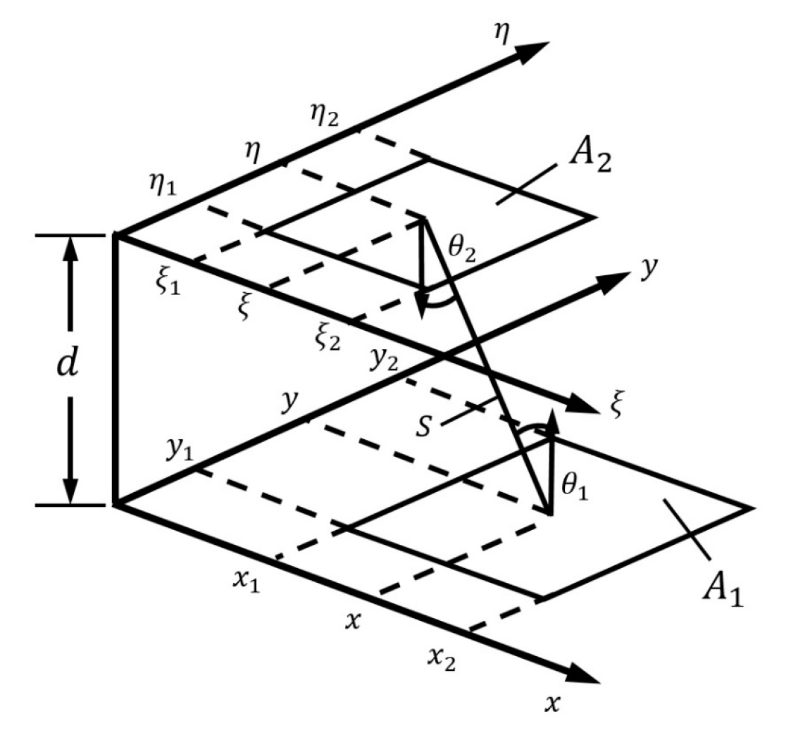
The relationship between the energy received by the second surface and the energy emitted by the first surface is known as the view factor. Mathematical equations for view factors are available for the relative positions of the surfaces [31,38]. The analytical view factor for two parallel, unequal, and non-coaxial rectangle plates is shown in Figure 5 and is given by Equation (7) [32]. In this equation, ( x 1 , y 1 ) , ( x 1 , y 2 ) , ( x 2 , y 1 ) , and ( x 2 , y 2 ) represent the coordinates of the vertices of plane A 1 and ( ξ 1 , η 1 ) , ( ξ 1 , η 2 ) , ( ξ 2 , η 1 ) , and ( ξ 2 , η 2 ) represent the coordinates of the vertices of plane A 2 . These two planes are spaced apart by d .
F 1 2 = 1 ( x 2 x 1 ) ( y 2 y 1 ) l = 1 2 k = 1 2 j = 1 2 i = 1 2 ( 1 ) ( i + j + k + l ) G ( x i , y j , η k , ξ l )
G ( x i , y j , η k , ξ l ) = 1 2 π { ( y j η k ) ( x i ξ l ) 2 + d 2 tan 1 ( y j η k ( x i ξ l ) 2 + d 2 ) } + 1 2 π { ( x i ξ l ) ( y j η k ) 2 + d 2 tan 1 ( x i ξ l ( y j η k ) 2 + d 2 ) } d 2 4 π ln { ( x i ξ l ) 2 + ( y j η k ) 2 + d 2 }
Here, G ( x i , y j , η k , ξ l ) can be derived from the Equation (8).
With the element’s heat flow in all directions, it is possible to calculate the net heat flow, which is equivalent to the change in the element’s internal energy [18]. We discretize in time using the integer p as t = p Δ t . Hence, the time derivative is in terms of the difference in temperatures at new time ( p + 1 ) and previous time ( p ) , separated by the time interval Δ t according to Equation (9).
T t | m , n = T m , n p + 1 T m , n p Δ t
By substituting Equation (9) in Equation (1), new nodal temperatures at new time step ( p + 1 ) can be obtained through Equation (10).
T m , n p + 1 = T m , n p + α . Δ t ( T m + 1 , n p + T m 1 , n p 2 T m , n p ( Δ x ) 2 + T m , n + 1 p + T m , n 1 p 2 T m , n p ( Δ y ) 2 + 1 k ( ( h t p + h b p ) d ( T ambient T m , n p ) + A h ε e σ Δ x Δ y d [ h = 1 H F h m , n (   ( θ h p ) 4 ( T m , n p ) 4 )   ] ) )
Equations are explicit since the unknown nodal temperatures at time ( p + 1 ) are determined with known temperatures at time ( p ) in each time step. The initial condition at t = 0 when p = 0 for temperature of each node on thermoplastic sheet is equal to ambient temperature T ( x , y , 0 ) = T ambient . Moreover, since the thermoplastic is being kept inside a clamp frame and the thermal conductivity of thermoplastic is very low, the temperature of all elements around the sheet in touch with the clamp were considered constant and the boundary condition is T ( 0 , y , t ) t = T ( l , y , t ) t = T ( x , 0 , t ) t = T ( x , w , t ) t = 0 where l and w are the length and width of the sheet, respectively.

3. Laboratory-Scale Setup

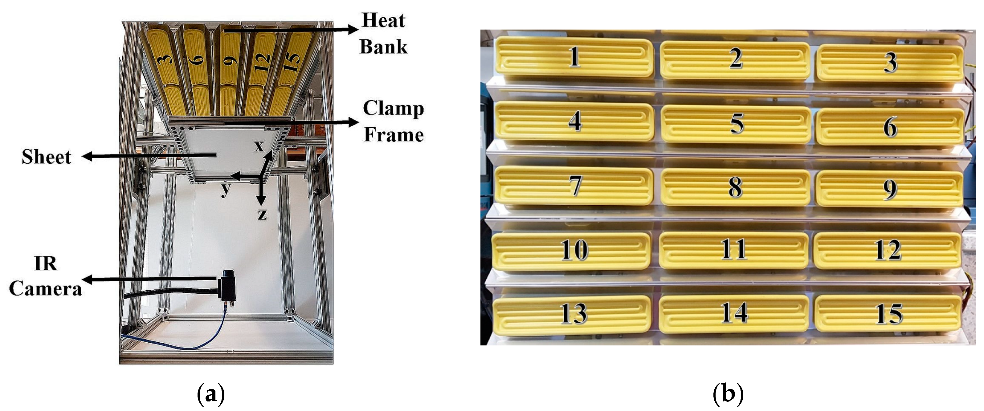
A laboratory-scale thermoforming setup is constructed to collect calibration data and validate the developed model. The heat bank consists of fifteen trough ceramic heating elements of 500 W and is located on the sheet’s top surface in five rows and three columns according to Figure 6. To measure the sheet’s surface temperature distribution, an infrared (IR) camera is installed underneath the sheet Figure 6a.
The clamp frame’s distance from the heat bank is movable. Each heating element’s electrical power consumption ranges from 0 to 500 W, and depending on the heater’s electrical power consumption, its surface temperature can reach a saturated temperature level from ambient temperature to 803 K. The thermoplastic sheet is placed on the mold for vacuum processing once the desired temperature profile is created on the sheet. The clamp frame is 500 mm by 320 mm in size, and thermoplastic sheets of the same size can be placed inside of it. To prevent wasted radiation from behind and to concentrate radiation on the sheet, the heating elements are fitted with reflectors. Figure 6a depicts the main axis of the sheet as well as the number and location of the heating elements. To model the heating element’s dynamics, we must examine the surface temperature variation of the heaters for different power consumptions. In addition, the actual radiation pattern of the ceramic heater needs to be determined. The experimental view factor matrix is then incorporated into the radiation heat transfer equation to improve the accuracy of the model.

3.1. Heating Element’s Surface Temperature Variation Modelling

Obtaining a precise model of the surface temperature variation of heating elements in relation to the input electrical power is an essential component of our thermal model. The surface temperature variation of the heating element is measured over time using an infrared (IR) camera at different power consumption levels. The heating and cooling rates of the heater are highly dependent on the ambient temperature and heat transfer via convection. The following test is conducted at a 21-degrees Celsius ambient temperature in a laboratory setting with minimal air flow. Figure 7a shows the variation in surface temperature of the trough ceramic heating element (500 W) with nine different power levels over time. Each curve displays the characteristics of a first-order transfer function according to Equation (11). Any first-order system can be described completely using two parameters: the steady-state gain K, and the time constant τ .
θ ( s ) u ( s ) = K τ s + 1
However, the steady-state gain K and time constant τ for our heating elements depend on the input power. To represent the variation in K and τ with respect to the duty cycle, the best-fit second-order polynomial function was used. The first order model’s output and the actual surface temperature variation of the trough ceramic heating element are compared in Figure 7b. The relative average error for the first order heater model is approximately 4%, according to its definition in Equation (12) where N is the number of samples along a curve. It should be noted that even though the model was developed for the heating process, it also performs well for the cooling process.
e ¯ r = [ 1 N i = 1 N ( | θ actual θ model | θ actual ) i ] × 100

3.2. Experiment to Determine Heating Element’s Radiation Pattern

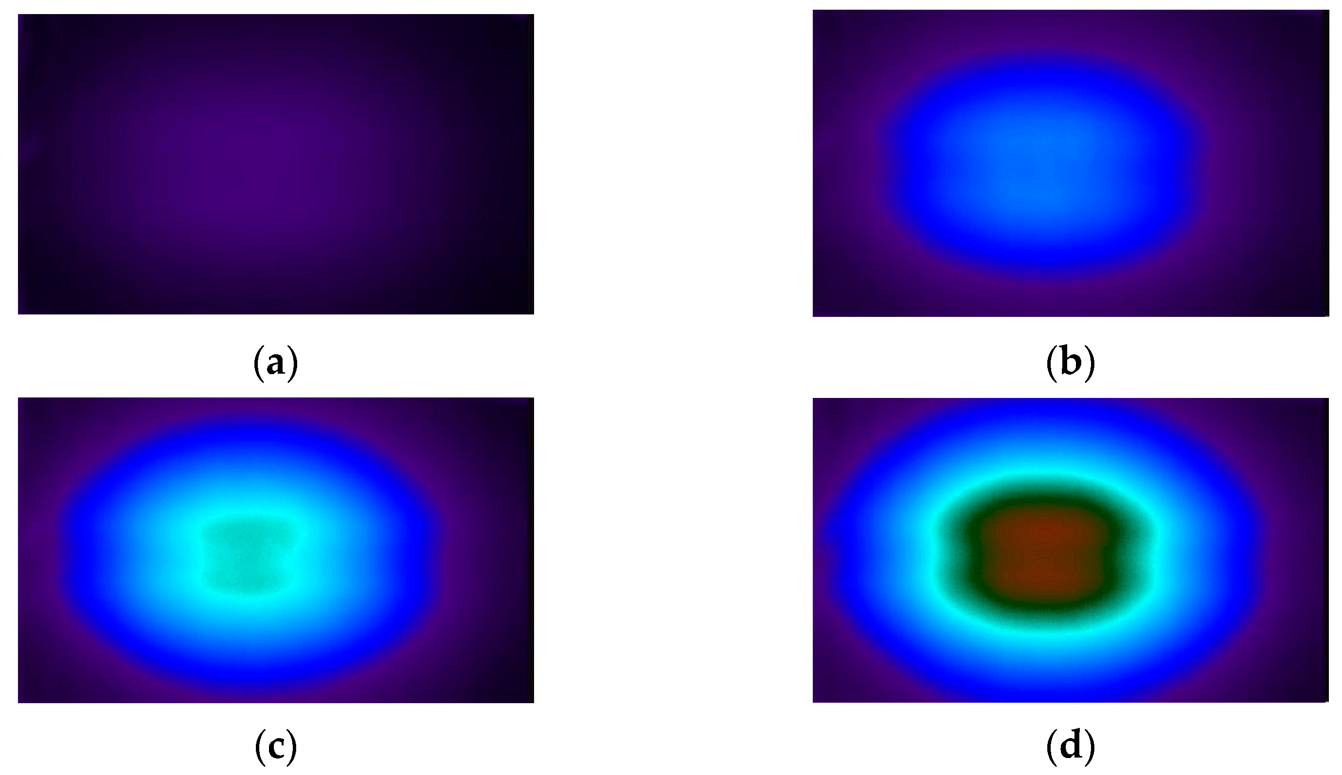
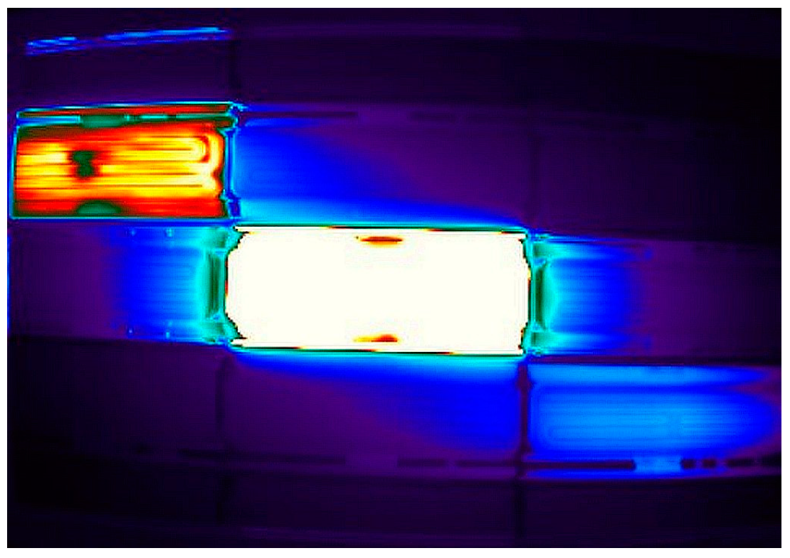
The 2D models of the heating phase in the thermoforming process that have been developed using analytical equations for the view factor assume that the heating element is a flat, temperature-maintaining plate. However, in practice, the radiation pattern varies significantly based on the geometry of the heating element. Given the trough ceramic heating coil that has been used in the laboratory-scale setup, an experiment is conducted to determine the exact view factor matrix between the trough ceramic heating coil and the sheet elements. The saturated surface temperature for a trough ceramic heating element at its maximum electrical power level of 500 W is 803 K. Figure 8 depicts the resulting temperature distribution variation on a thermoplastic sheet located at a distance of 15 cm from heater number 8 (in Figure 6b) over a 60 s interval.
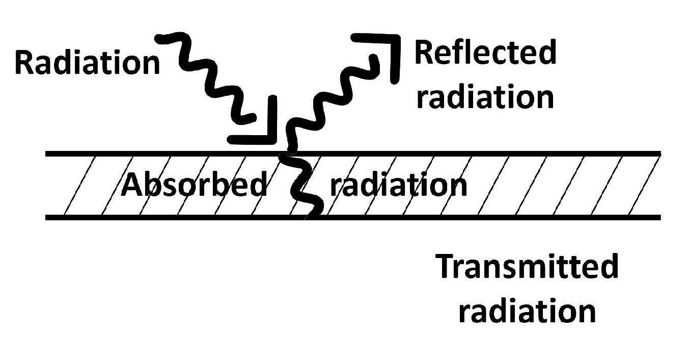
Considering the small distance between the sheet and heating element, furthermore, because of the use of reflectors behind each heater, we assume that all the radiation from the heating coil that is located in the center of the thermoplastic sheet (Heater number 8 in Figure 6b) strikes the surface of the sheet. Some thermoplastics, such as polycarbonate and acrylic, are highly transparent, while PVC and ABS are opaque. Since an opaque acrylic thermoplastic sheet loaded with a specific amount of pigment is used in our experiment (Figure 6a), all infrared emissions are considered either reflected ( ρ r ), or absorbed ( α a ) by the thermoplastic sheet (Figure 9). There is a straightforward relationship between these two variables according to equation 13 that totals 1 or 100 percent. For a black surface, which absorbs all incoming radiation and emits the maximum possible, α a = 1 and ρ r = 0 [36].
ρ r + α a = 1
Taking into account the thermoplastic’s low thermal conductivity and the low thermal loss through convection when the sheet’s temperature is low, by ignoring the conduction and convection parts in Equation (10) and using only one heater in the center of the sheet (heater number 8 in in Figure 6b) the product of the view factor between the elements of the sheet and the heater and the absorptivity of the sheet can be calculated at the initial heating time using Equation (14). The emissivity for the ceramic heater ( ε h ) in the setup is 0.92 [39].
α a F h m , n = k Δ x Δ y d α A h ε e σ (   ( θ h p ) 4 ( T m , n p ) 4 ) × ( T m , n p + 1 T m , n p Δ t )
Figure 10 shows the extracted experimental α a × F h m , n for each element of the sheet using Equation (14) and the thermal and physical properties of thermoplastic shown in Table 1. As can be seen, the elements located under the heater receive a larger portion of the emitted energy by heater.
Considering the summation of view factors rule and the superposition rule, if the sheet is divided into M × N equal elements, the view factor from the heater to the sheet is equal to sum of all view factors from the heater to the elements of the sheet. We assumed that all radiation of the heating coil strikes the surface of the sheet. Hence, according to Equation (15) the summation of view factors from the heater to the elements of the sheet is equal to 1.
F heater sheet = m = 1 M n = 1 N F heater m , n = 1
The total α a × F h m , n of all elements in Figure 10 is 0.55. If the absorptivity is assumed the same in all elements on the sheet. According to Equations (15) and (16), the total product of view factor between the elements of the sheet and the heater and absorptivity of the sheet will equal to αa, indicating that approximately 45 percent of the emitted energy is reflected by the thermoplastic sheet due to the white and smooth surface of it.
m = 1 M n = 1 N α a F heater m , n = α a m = 1 M n = 1 N F heater m , n = α a

4. Model Verification and Results

A laboratory-scale setup is used to validate the designed heating phase model. A test scenario with the initial condition specified in Table 2 ran for two minutes. As can be seen in Figure 11, only heating elements 4 and 8 received 200 W and 500 W of electrical power, respectively.
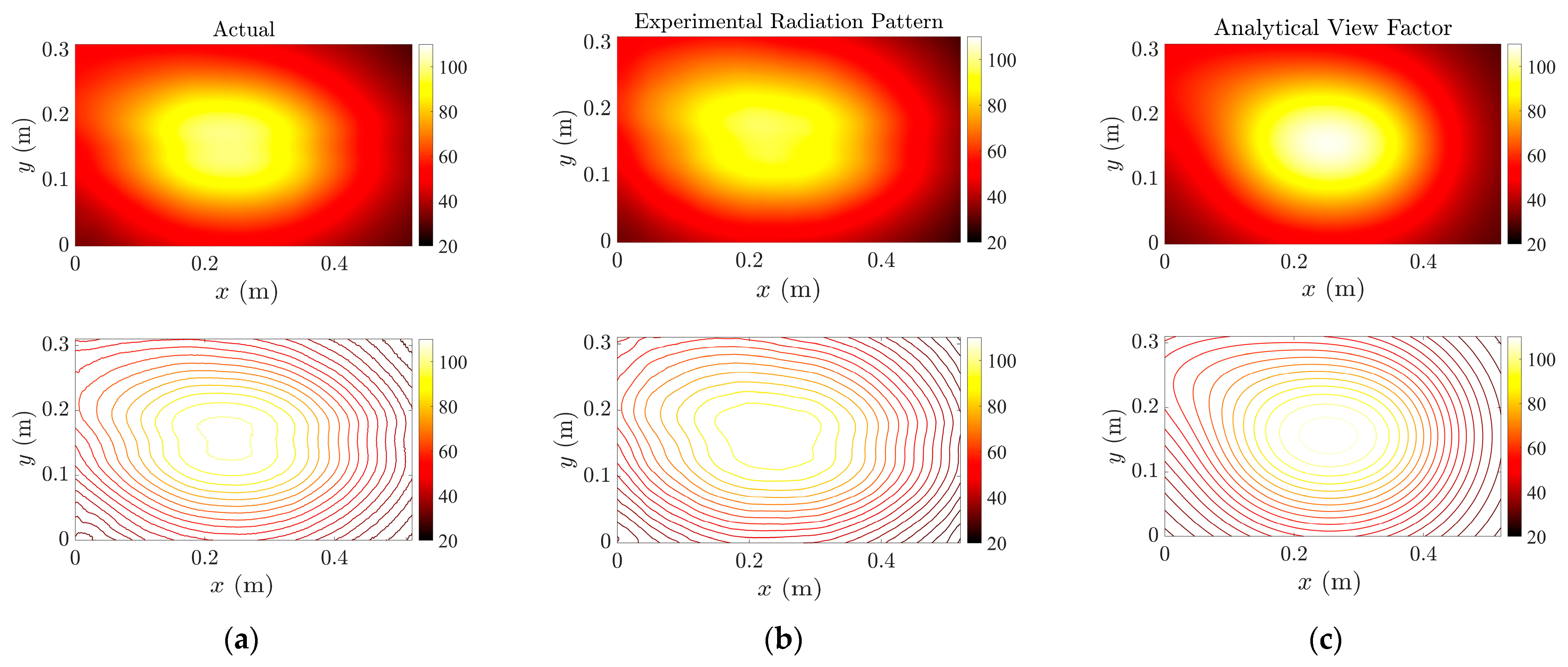
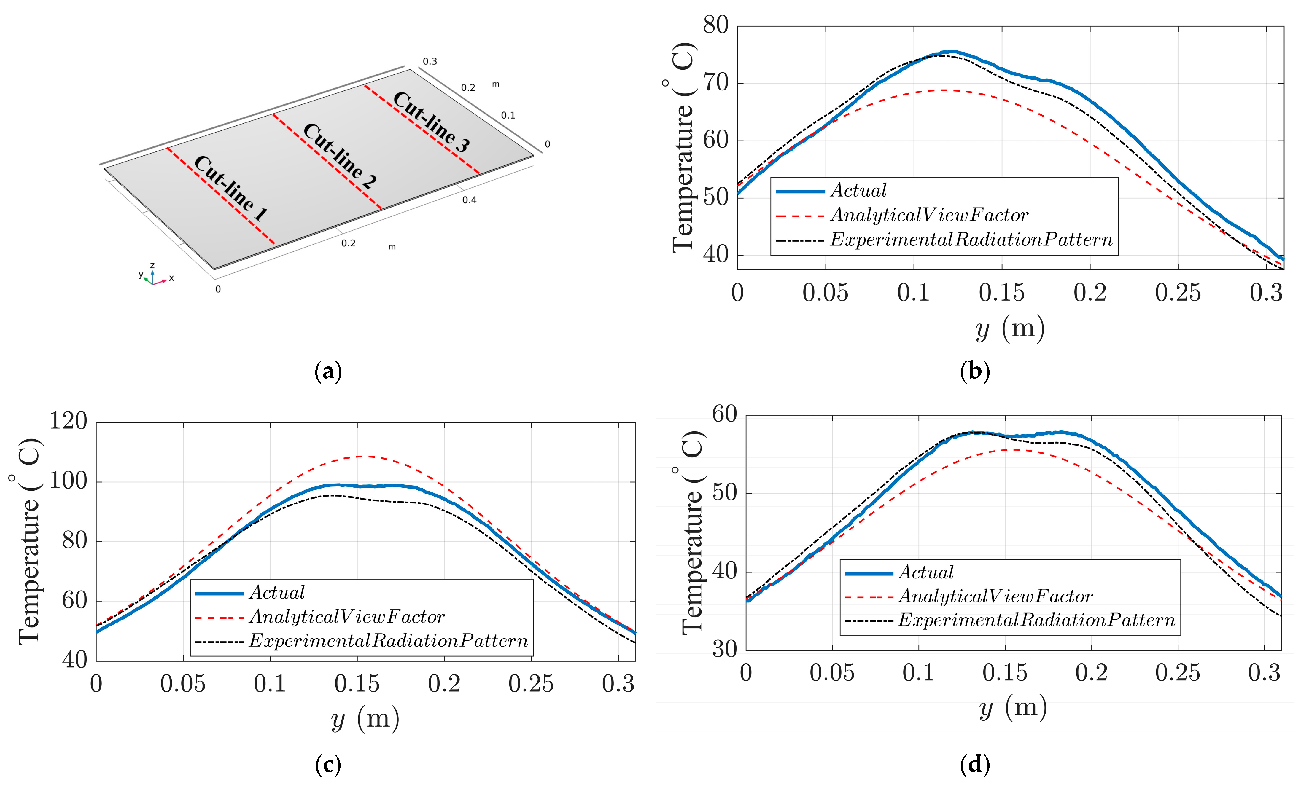
Figure 12 compares the actual and predicted temperature distribution on the thermoplastic sheet after 120 s. Clearly, the model based on measured view factors (Figure 12b) provides a better temperature distribution than the traditional analytical model based on flat plates (Figure 12c). Three cut-lines are applied in the x and y directions of the sheet as shown in Figure 13a and Figure 14a to better compare the temperature variation between the actual heated sheet and the model’s output. Figure 13b–d and Figure 14b–d compare the variation in actual and simulated temperatures on the sheet along these cut-lines.
To assess the accuracy of the designed model along these cut-lines, the Mean Squares Error (MSE) and Root Mean Squares Error (RMSE) were calculated using Equations (17) and (18). Table 3 lists the MSE and RMSE along six cut-lines in model using two different methods. Comparing the proposed method’s performance to that of the same model when utilizing the analytical method [32] to calculate the view factors demonstrates that the proposed method performs significantly better.
MSE = 1 N i = 1 N ( T actual T model ) 2 i
RMSE = MSE = 1 N i = 1 N ( T actual T model ) 2 i
Figure 15 depicts the implementation of the same scenario in the COMSOL software [40] to compare the speed of the designed model. Given the configuration of computation hardware, it was impractical to implement the actual geometry of heating elements. As a result, a flat plate model of heaters equivalent to the analytical view factors was implemented. Despite the implementation of a simple model of heating elements, the scenario required 480 s to be computed by the COMSOL software. Comparing the 45 s computation time of the designed model for this scenario with the same configuration of computation hardware reveals that the designed model is nearly ten times faster.

5. Discussion and Conclusions

In order to study the temperature distribution on the thermoplastic sheet, a 2D model of the heating phase of the thermoforming process is developed in this paper. In 3D models, it is possible to implement the precise geometry of the heating elements and, as a result, account for the actual radiation pattern of the heaters on the sheet. Due to the enormous computational effort required by these models, it is impractical to use them in model-free control strategies such as reinforcement learning, which requires a large number of “trial and error” episodes or interactions with the model to train the algorithm. Although 2D models of the heating phase of the thermoforming process are computationally efficient, they assume the heating element is a flat plate and employ analytical view factor relations. This assumption creates a discrepancy between the model and the actual output radiation pattern of the heater. The method proposed in this paper for developing a 2D model of the thermoforming heating phase demonstrates that the designed model reduces the MSE and RMSE by four and two times, respectively, compared to conventional 2D models based on the analytical view factor. Moreover, despite the implementation of a simple heating element model in the COMSOL software, a comparison of the computation times of the designed model and the COMSOL software for this scenario with the same configuration of computation hardware reveals that the designed model is almost ten times faster. As potential next steps, the presented heat transfer model can be integrated to larger process modeling and optimization platforms, e.g., to migrate (thermo)forming induced wrinkles [41]. Non-local modeling [42] of the forming sheet may also be worthwhile to account for different material scales within the composite structure.

Author Contributions

The conceptualization, methodology, software, visualization, validation and writing the original draft are performed by H.H. Resources, data curation, and investigation are conducted by M.R. The tasks of supervision, review and editing, and formal analysis are performed by R.S. Funding acquisition and project administration are conducted by A.S.M. All authors have read and agreed to the published version of the manuscript.

Funding

This research was funded by the New Frontiers in Research Fund (NFRF) of Canada, grant number: NFRFE-2019-01440.

Data Availability Statement

Not applicable.

Acknowledgments

The authors would like to thank Iman Jalilvand and Rohith J.K. for their assistance and insightful feedback regarding the integration of the laboratory-scale thermoforming setup at the University of British Columbia.

Conflicts of Interest

The authors declare no conflict of interest.

References

  1. Rosin, F.; Forget, P.; Lamouri, S.; Pellerin, R. Enhancing the Decision-Making Process through Industry 4.0 Technologies. Sustainability 2022, 14, 461. [Google Scholar] [CrossRef]
  2. Forbes, M.G.; Patwardhan, R.S.; Hamadah, H.; Gopaluni, R.B. Model Predictive Control in Industry: Challenges and Opportunities. IFAC-PapersOnLine 2015, 48, 531–538. [Google Scholar] [CrossRef]
  3. Ramezankhani, M.; Narayan, A.; Seethaler, R.; Milani, A.S. An Active Transfer Learning (ATL) Framework for Smart Manufacturing with Limited Data: Case Study on Material Transfer in Composites Processing. In Proceedings of the 2021 4th IEEE International Conference on Industrial Cyber-Physical Systems (ICPS), Victoria, BC, Canada, 10–12 May 2021; pp. 277–282. [Google Scholar] [CrossRef]
  4. Ramezankhani, M.; Crawford, B.; Narayan, A.; Voggenreiter, H.; Seethaler, R.; Milani, A.S. Making costly manufacturing smart with transfer learning under limited data: A case study on composites autoclave processing. J. Manuf. Syst. 2021, 59, 345–354. [Google Scholar] [CrossRef]
  5. Nian, R.; Liu, J.; Huang, B. A review On reinforcement learning: Introduction and applications in industrial process control. Comput. Chem. Eng. 2020, 139, 106886. [Google Scholar] [CrossRef]
  6. McClement, D.G.; Lawrence, N.P.; Loewen, P.D.; Forbes, M.G.; Backström, J.U.; Gopaluni, R.B. A Meta-Reinforcement Learning Approach to Process Control. IFAC-PapersOnLine 2021, 54, 685–692. [Google Scholar] [CrossRef]
  7. McClement, D.G.; Lawrence, N.P.; Backström, J.U.; Loewen, P.D.; Forbes, M.G.; Gopaluni, R.B. Meta reinforcement learning for adaptive control: An offline approach. Submitt. J. Process Control. 2022. [Google Scholar] [CrossRef]
  8. Throne, J.L. (Ed.) Understanding Thermoforming. In Understanding Thermoforming, 2nd ed.; Hanser: München, Wien, 2008; pp. I–XIII. [Google Scholar]
  9. Throne, J.L. Technology of Thermoforming; Hanser Gardner Publications: Munich, Germany, 1996. [Google Scholar]
  10. Leite, W.D.O.; Campos Rubio, J.C.; Mata Cabrera, F.; Carrasco, A.; Hanafi, I. Vacuum Thermoforming Process: An Approach to Modeling and Optimization Using Artificial Neural Networks. Polymer 2018, 10, 143. [Google Scholar] [CrossRef]
  11. Hosseini, H.; Berdyshev, B.V.; Mehrabani-Zeinabad, A. Modeling of Deformation Processes in Vacuum Thermoforming of a Pre-stretched Sheet. Polym. Technol. Eng. 2006, 45, 1357–1362. [Google Scholar] [CrossRef]
  12. Wang, P.; Hamila, N.; Boisse, P. Thermoforming simulation of multilayer composites with continuous fibres and thermoplastic matrix. Compos. Part B Eng. 2013, 52, 127–136. [Google Scholar] [CrossRef]
  13. Xiong, H.; Hamila, N.; Boisse, P. Consolidation Modeling during Thermoforming of Thermoplastic Composite Prepregs. Materials 2019, 12, 2853. [Google Scholar] [CrossRef] [PubMed]
  14. Wang, H.; Li, X.; Phipps, M.; Li, B. Numerical and experimental study of hot pressing technique for resin-based friction composites. Compos. Part A Appl. Sci. Manuf. 2022, 153, 106737. [Google Scholar] [CrossRef]
  15. Wagner, S.; Kayatz, F.; Münsch, M.; Sanjon, C.W.; Hauptmann, M.; Delgado, A. Numerical modeling of forming air impact thermoforming. Int. J. Adv. Manuf. Technol. 2022, 120, 4917–4933. [Google Scholar] [CrossRef]
  16. Bean, P.; Lopez-Anido, R.A.; Vel, S. Integration of Material Characterization, Thermoforming Simulation, and As-Formed Structural Analysis for Thermoplastic Composites. Polymers 2022, 14, 1877. [Google Scholar] [CrossRef] [PubMed]
  17. Buffel, B.; van Mieghem, B.; van Bael, A.; Desplentere, F. A Combined Experimental and Modelling Approach towards an Optimized Heating Strategy in Thermoforming of Thermoplastics Sheets. Int. Polym. Process. 2017, 32, 378–386. [Google Scholar] [CrossRef]
  18. Wilson, J.; Everett, S.; Dubay, R.; Parsa, S.S.; Tyler, M. Spatial predictive control using a thermal camera as feedback. Measurement 2017, 109, 384–393. [Google Scholar] [CrossRef]
  19. Shen, Y.-D.; Li, Z.-Z.; Xuan, D.-J.; Heo, K.-S.; Seol, S.-Y. Time-dependent optimal heater control using analytic and numerical methods. Int. J. Precis. Eng. Manuf. 2010, 11, 77–81. [Google Scholar] [CrossRef]
  20. Li, Z.-Z.; Ma, G.; Xuan, D.-J.; Seol, S.-Y.; Shen, Y.-D. A study on control of heater power and heating time for thermoforming. Int. J. Precis. Eng. Manuf. 2010, 11, 873–878. [Google Scholar] [CrossRef]
  21. Erchiqui, F.; Hamani, I.; Charette, A. Modélisation par éléments finis du chauffage infrarouge des membranes thermoplastiques semi-transparentes. Int. J. Therm. Sci. 2009, 48, 73–84. [Google Scholar] [CrossRef]
  22. Venkateswaran, G.; Cameron, M.R.; Jabarin, S.A. Effects of temperature profiles through preform thickness on the proper-ties of reheat-blown PET containers. Adv. Polym. Technol. 1998, 17, 237–249. [Google Scholar] [CrossRef]
  23. Schmidt, F.; Le Maoult, Y.; Monteix, S. Modelling of infrared heating of thermoplastic sheet used in thermoforming process. J. Mater. Process. Technol. 2003, 143-144, 225–231. [Google Scholar] [CrossRef]
  24. Duarte, F.; Covas, J.A. IR sheet heating in roll fed thermoforming: Part 1—Solving direct and inverse heating problems. Plast. Rubber Compos. 2002, 31, 307–317. [Google Scholar] [CrossRef]
  25. Duarte, F.; Covas, J.A. Infrared sheet heating in roll fed thermoforming: Part 2—Factors influencing inverse heating solution. Plast. Rubber Compos. 2003, 32, 32–39. [Google Scholar] [CrossRef]
  26. Monteix, S.; Schmidt, F.; Le Maoult, Y.; Ben Yedder, R.; Diraddo, R.; Laroche, D. Experimental study and numerical simulation of preform or sheet exposed to infrared radiative heating. J. Mater. Process. Technol. 2001, 119, 90–97. [Google Scholar] [CrossRef]
  27. Yousefi, A.; Bendada, A.; Diraddo, R. Improved modeling for the reheat phase in thermoforming through an uncertainty treatment of the key parameters. Polym. Eng. Sci. 2002, 42, 1115–1129. [Google Scholar] [CrossRef]
  28. Gauthier, G.; Ajersch, M.; Boulet, B.; Haurani, A.; Girard, P.; Diraddo, R. A new absorption based model for sheet reheat in thermoforming. In Annual Technical Conference; ANTEC: Boston, MA, USA, 2005. [Google Scholar]
  29. Chy, M.I.; Boulet, B. Development of an improved mathematical model of the heating phase of thermoforming process. In Proceedings of the 2011 IEEE Industry Applications Society Annual Meeting, Orlando, FL, USA, 9–13 October 2011; pp. 1–8. [Google Scholar] [CrossRef]
  30. Erchiqui, F. Application of genetic and simulated annealing algorithms for optimization of infrared heating stage in thermoforming process. Appl. Therm. Eng. 2018, 128, 1263–1272. [Google Scholar] [CrossRef]
  31. Erchiqui, F.; Ngoma, G.D. Analyse comparative des méthodes de calcul des facteurs de formes pour des surfaces à contours rectilignes. Int. J. Therm. Sci. 2007, 46, 284–293. [Google Scholar] [CrossRef]
  32. Ehlert, J.R.; Smith, T.F. View factors for perpendicular and parallel rectangular plates. J. Thermophys. Heat Transf. 1993, 7, 173–175. [Google Scholar] [CrossRef]
  33. Rodrigues, J.D.S.; Gonçalves, P.T.; Pina, L.; de Almeida, F.G. Modelling the Heating Process in the Transient and Steady State of an In Situ Tape-Laying Machine Head. J. Manuf. Mater. Process. 2022, 6, 8. [Google Scholar] [CrossRef]
  34. Holman, J.P. Heat Transfer; McGraw-Hill: New York, NY, USA, 2009. [Google Scholar]
  35. Poelma, R.H.; Tarashioon, S.; Van Zeijl, H.W.; Goldbach, S.; Zijl, J.L.J.; Zhang, G.Q. Multi-LED package design, fabrication and thermal analysis. J. Semicond. 2013, 34, 54002. [Google Scholar] [CrossRef]
  36. Michael, F. Modest: Radiative Heat Transfer; Elsevier: Amsterdam, The Netherlands, 2003. [Google Scholar]
  37. Howell, J.R.; Mengüç, M.P.; Daun, K.; Siegel, R. Thermal Radiation Heat Transfer, 7th ed.; CRC Press: Boca Raton, FL, USA, 2021; Revised edition of: Thermal radiation heat transfer/John R. Howell, M. Pinar Mengüç, Robert Siegel; Sixth edition. 2015. (2020). [Google Scholar]
  38. Ivanova, S.M.; Muneer, T. Finite-element heat-transfer computations for parallel surfaces with uniform or non-uniform emitting. J. Renew. Sustain. Energy 2016, 8, 015102. [Google Scholar] [CrossRef]
  39. Ceramicx Company. Available online: https://www.ceramicx.com/ (accessed on 1 September 2022).
  40. COMSOL. Multiphysics® v. 5.6; COMSOL AB: Stockholm, Sweden; Available online: www.comsol.com (accessed on 1 September 2022).
  41. Rashidi, A.; Milani, A.S. Passive control of wrinkles in woven fabric preforms using a geometrical modification of blank holders. Compos. Part A Appl. 2018, 105, 300–309. [Google Scholar] [CrossRef]
  42. Daghigh, H.; Daghigh, V.; Milani, A.; Tannant, D.; Lacy, V.C., Jr.; Reddy, N.J. Nonlocal bending and buckling of agglomerated CNT-reinforced composite nanoplates. Compos. B. Eng. 2020, 183, 107716. [Google Scholar] [CrossRef]
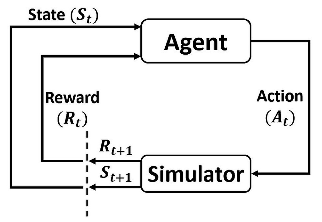
Figure 1. The general reinforcement learning framework.
Jmmp 07 00048 g001
Figure 2. Schematic of basic vacuum thermoforming. (a) Heating; (b) sealing or pre-stretch; (c) forming and cooling [4].
Jmmp 07 00048 g002
Figure 3. (a) Heat transfer between thermoplastic sheet, radiant heaters, and ambient; (b) elements for model.
Jmmp 07 00048 g003
Figure 4. Heat transfer coefficient for free convection between the cold surrounding and hot plate [35].
Jmmp 07 00048 g004
Figure 5. Plate arrangements (parallel plates) [32].
Jmmp 07 00048 g005
Figure 6. (a) Laboratory-scale heating system setup; (b) number of heating elements.
Jmmp 07 00048 g006
Figure 7. (a) Actual heater surface temperature variation over time for different power levels; (b) comparison the simulated and actual surface temperatures variation over time in different power consumption.
Jmmp 07 00048 g007
Figure 8. Laboratory-scale setup: temperature distribution on the sheet using a trough ceramic heater with 500 W maximum power consumption at (a) t = 15 s; (b) t = 30 s; (c) t = 45 s; (d) t = 60 s.
Jmmp 07 00048 g008
Figure 9. Reflected and absorbed radiation on opaque surface.
Jmmp 07 00048 g009
Figure 10. Extracted experimental α a × F h m , n for each element of the sheet (a) surface graph; (b) numerical values of α a × F h m , n in contour graph.
Jmmp 07 00048 g010
Figure 11. Heating elements number 4 and 8 with surface temperature of 603 K and 803 K, respectively.
Jmmp 07 00048 g011
Figure 12. Temperature distribution on the sheet (a) laboratory-scale setup; (b) designed model based on experimental radiation pattern; (c) designed model based on analytical view factors.
Jmmp 07 00048 g012
Figure 13. Actual and simulated temperature variations along three cut-line in the y direction of the thermoplastic sheet, (a) cut-line locations; (b) cut-line 1 temperatures; (c) cut-line 2 temperatures; (d) cut-line 3 temperatures.
Jmmp 07 00048 g013
Figure 14. Actual and simulated temperature variations along three cut-line in the x direction of the thermoplastic sheet, (a) cut-line locations; (b) cut-line 1 temperatures; (c) cut-line 2 temperatures; (d) cut-line 3 temperatures.
Jmmp 07 00048 g014
Figure 15. Temperature distribution on the sheet after 120 s (COMSOL Multiphysics V 5.6 software).
Jmmp 07 00048 g015
Table 1. Thermal and physical properties for thermoplastic sheet.
DirectionSymbolValueUnit
Thermal Conductivity K 0.18 ( W / m . K )
Specific Heat c p 1465 ( J / kg   K )
Density Ρ 1380 ( kg / m 3 )
Emissivity ε s 0.95-
Table 2. Initial condition of heating elements for test.
#HeaterPower Consumption (W)Heaters’ Surface Temperature (K)
4200603
8500803
Table 3. Comparison of mean square errors along six cut-line in two methods.
Vertical Cut-LinesHorizontal Cut-Lines
Experimental Radiation PatternAnalytical View FactorsExperimental Radiation PatternAnalytical View Factors
MSERMSEMSERMSEMSERMSEMSERMSE
Cut-line 14.32.0722.24.715.52.3416.24.02
Cut-line 210.43.2223.74.863.81.9440.56.36
Cut-line 32.41.545.72.383.41.8416.84.09
Disclaimer/Publisher’s Note: The statements, opinions and data contained in all publications are solely those of the individual author(s) and contributor(s) and not of MDPI and/or the editor(s). MDPI and/or the editor(s) disclaim responsibility for any injury to people or property resulting from any ideas, methods, instructions or products referred to in the content.