
Machine Learning Application Using Cost-Effective Components for Predictive Maintenance in Industry: A Tube Filling Machine Case Study


Abstract
:1. Introduction
- The system made was a prototype that was chosen using cost-efficient materials;
- The system will use two supervised machine learning methods to compare the effectivity of random forest regression and linear regression;
- The system will trace failure based on a failure that made the product rejected or downtime;
- The system will ignore a failure that consists of human error;
- The machine is operating for a maximum of 16 h a day.
2. Materials and Methods
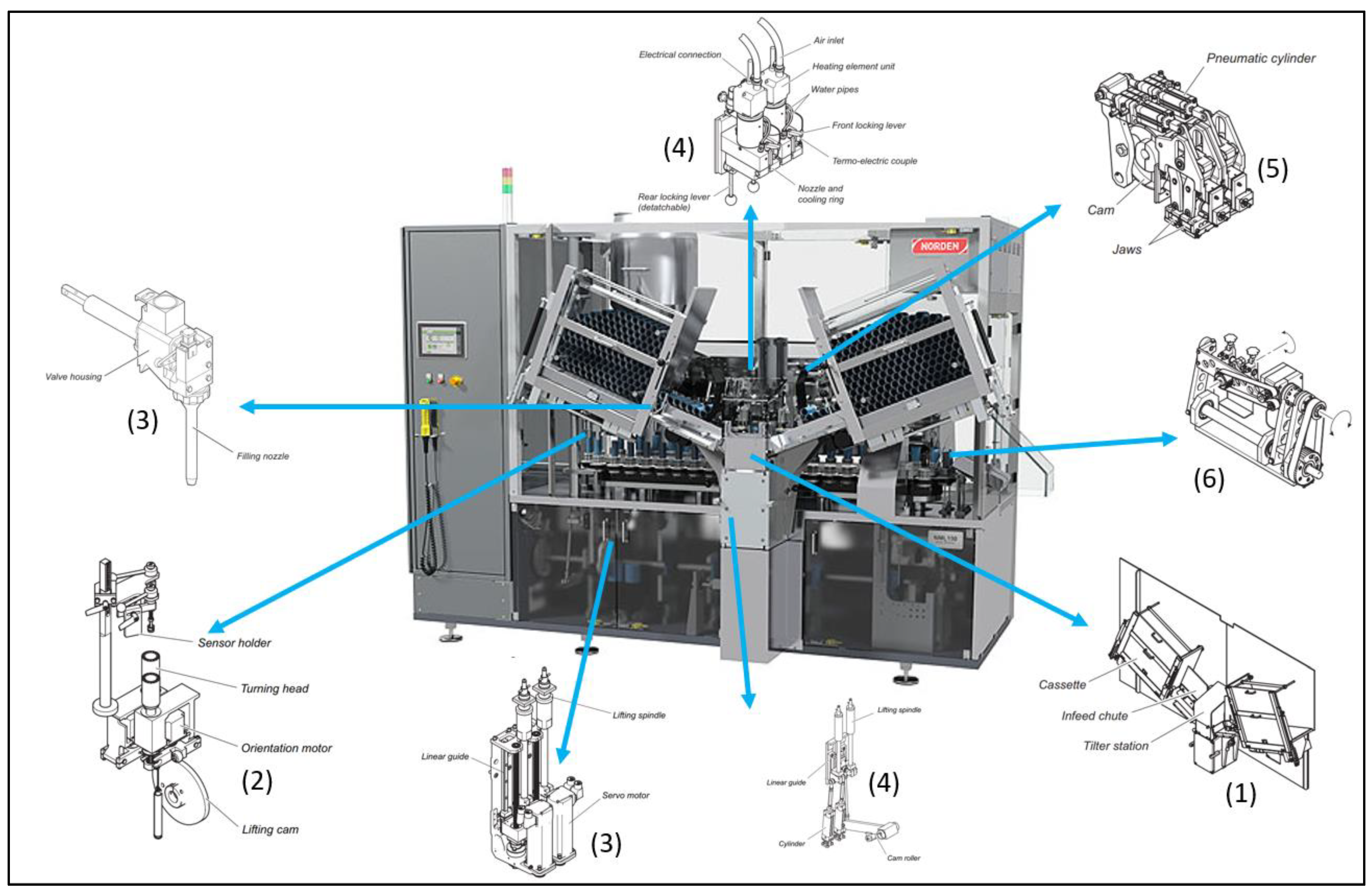
2.1. Experimental Setup
2.2. Components and Sensor Placement
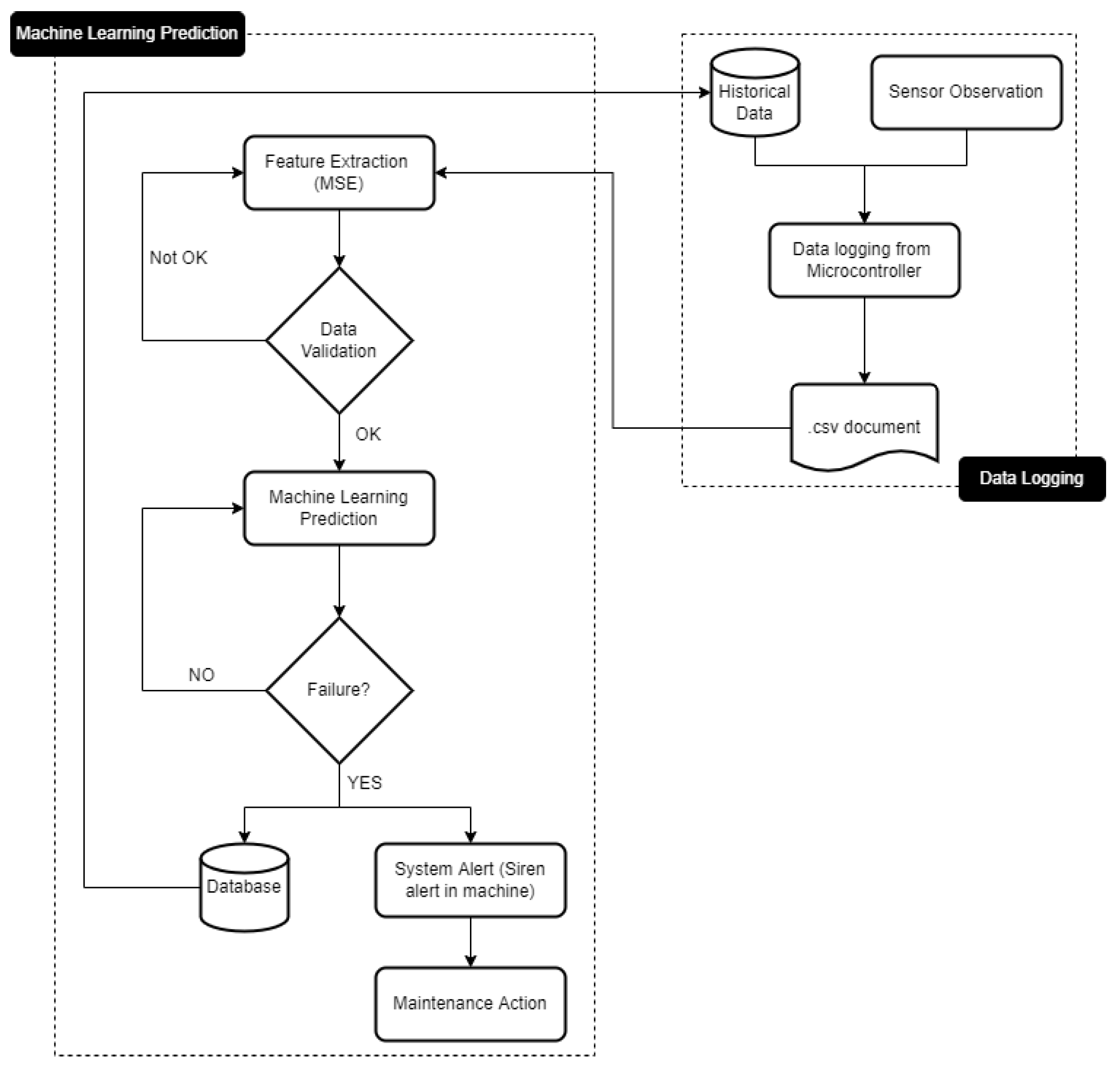
2.3. Method and Algorithm
| Algorithm 1. Data Logging Algorithm | |||
| Require | : | ||
| Ensure | : | ‣ Starting data count from 0 | |
| ‣ Ensure the value between Max and Min | |||
| While do | |||
| If is running then | |||
| ‣ N = Number of Sensors Port | |||
| Else if is stop then | |||
| ‣ .csv stop working | |||
| End if | |||
| End While | |||
- Spacing for each column will be separated with a comma (default);
- The decimal value will use a dot (.) to specify the value;
- The timestamp algorithm will use a dash (-) separator.
| Algorithm 2. Machine Learning Prediction Algorithm | |||
| Require | : | ‣ There must be a data transfer process | |
| Ensure | : | ||
| Ensure | : | ‣ Number of repetition must | |
| While do | |||
| If is running then | |||
| If is available then | |||
| End if | |||
| ‣ Random forest reg. k = Rand State | |||
| Else If is stop then | |||
| ‣ .csv stop working | |||
| End if | |||
| End While | |||
- Feature extraction from the sample data using C++ open-source programs [39] by eliminating the noise from the acquired data (sensor position change and temperature change) from the data acquisition program;
- Data training using data from Table 4 and fitting data into the random forest and linear regression separately, with a total of 16 datasets, having been trained;
- From the total of 16 datasets, the optimal hyper-parameters are found using cross-validation of the k-sections method [19]. The method will randomly subdivide the examples data into “k” sections, and for each value of parameters, the learning algorithm is executed for “k” times [19]. For the best results, hyperparameters were used in the experiment, such as sample split 10, estimators 5500, and random state 40 (for random forest prediction). The results also agree with the research of Prihatno et al. in terms of humidity predictions [32];
- For better prediction results, means square error (MSE) and root mean square error (RMSE) are also calculated and fitted from 16 samples. The MSE and RMSE values are used to compare the training data accuracy with the real system data accuracy [40]. The results of MSE and RMSE from the training data can be seen in Table 6.
3. Results and Discussion
3.1. Machine Condition Monitoring
- Normal acceleration/vibration condition;
- Normal temperature condition;
- Run to Fail acceleration/vibration condition;
- Run to fail temperature condition.
3.2. Machine Learning Prediction Value
- RF Regression prediction using normal condition;
- RF Regression prediction using failure condition;
- LR prediction using normal condition;
- LR prediction using failure condition.
3.3. Failure Model and Effect Analysis for the System
4. Implementation Discussion
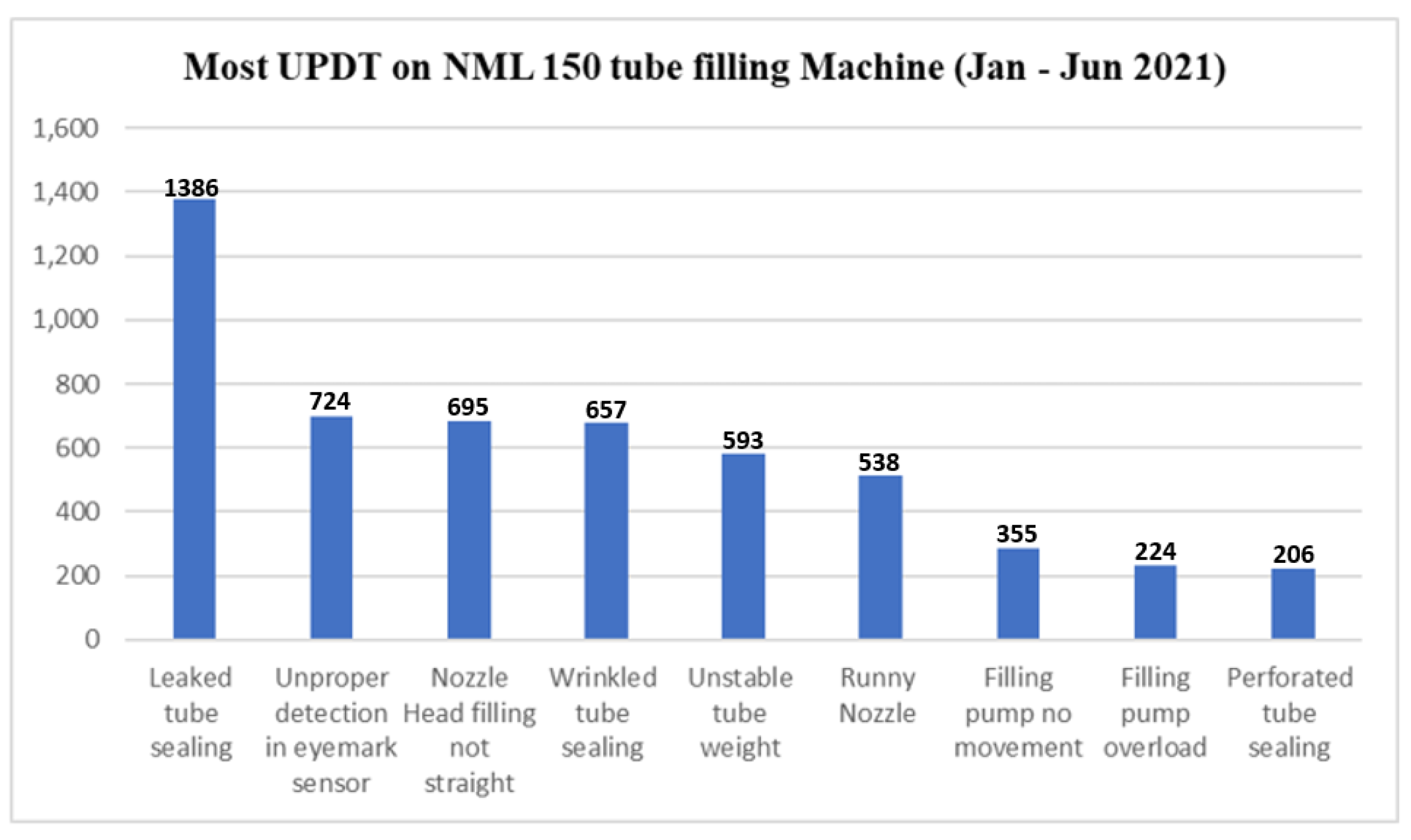
- Total machine UPDT comparison three months before and three months after;
- Targeted machine UPDT comparison three months before and three months after;
- Comparison of machine output three months before and three months after.
- Improvement in human resource/machine operator;
- Improvement in raw material qualities;
- Improvement in operational methods.
5. Conclusions
- Improve microcontroller and hardware for data acquisition with a higher baud rate and sampling rate to have more accuracy of the data and a faster processing time in algorithm run;
- Improvement in accelerometer and vibration sensor with a higher detection range and a higher sampling rate to make possible the fine-tuning of the system to obtain a faster failure prediction and a faster PdM action;
- For further recommendation, the system can predict another component, product reject detection and prediction, minimize human error in the operational machine, and synchronize the environmental conditions with machine parts conditions.
Author Contributions
Funding
Institutional Review Board Statement
Informed Consent Statement
Data Availability Statement
Acknowledgments
Conflicts of Interest
References
- Emovon, I.; Norman, R.A.; Murphy, A.J. Elements of maintenance system and tools for implementation within the framework of Reliability Centred Maintenance-A review. J. Mech. Eng. Technol. 2016, 8, 1–34. [Google Scholar]
- Saha, R.; Azeem, A.; Hasan, K.W.; Ali, S.M.; Paul, S.K. Integrated economic design of quality control and maintenance management: Implications for managing manufacturing process. Int. J. Syst. Assur. Eng. Manag. 2021, 12, 263–280. [Google Scholar] [CrossRef]
- Li, R.; Verhagen, W.J.; Curran, R. A systematic methodology for Prognostic and Health Management system architecture definition. Reliab. Eng. Syst. Saf. 2019, 193, 106598. [Google Scholar] [CrossRef]
- Cinar, Z.M.; Abdussalam Nuhu, A.; Zeeshan, Q.; Korhan, O.; Asmael, M.; Safaei, B. Machine Learning in Predictive Maintenance towards Sustainable Smart Manufacturing in Industry 4. Sustainability 2020, 12, 8211. [Google Scholar] [CrossRef]
- Calabrese, F.; Regattieri, A.; Bortolini, M.; Gamberi, M.; Pilati, F. Predictive Maintenance: A Novel Framework for a Data-Driven, Semi-Supervised, and Partially Online Prognostic Health Management Application in Industries. Appl. Sci. 2021, 11, 3380. [Google Scholar] [CrossRef]
- Chen, C.; Wang, C.; Lu, N.; Jiang, B.; Xing, Y. A data-driven predictive maintenance strategy based on accurate failure prognostics. Eksploat. Niezawodn. 2021, 23, 387–394. [Google Scholar] [CrossRef]
- Wang, K.; Wang, Y. How AI affects the future predictive maintenance: A primer of deep learning. In Proceedings of the International Workshop of Advanced Manufacturing and Automation, Singapore, 11 September 2017. [Google Scholar]
- Florian, E.; Sgarbossa, F.; Zennaro, I. Machine learning-based predictive maintenance: A cost-oriented model for implementation. Int. J. Prod. Econ. 2021, 236, 108114. [Google Scholar] [CrossRef]
- Selcuk, S. Predictive maintenance, its implementation and latest trends. Proc. Inst. Mech. Eng. Part B J. Eng. Manuf. 2017, 231, 1670–1679. [Google Scholar] [CrossRef]
- Baban, C.F.; Baban, M.; Suteu, M.D. Using a fuzzy logic approach for the predictive maintenance of textile machines. J. Intell. Fuzzy Syst. 2016, 30, 999–1006. [Google Scholar] [CrossRef]
- Misra, D.; Bennett, A.; Blukis, V.; Niklasson, E.; Shatkhin, M.; Artzi, Y. Mapping Instructions to Actions in 3D Environments with Visual Goal Prediction. Available online: https://arxiv.org/abs/1809.00786 (accessed on 4 August 2022).
- Setiawan, A.; Silitonga, R.Y.; Angela, D.; Sitepu, H.I. The Sensor Network for Multi-agent System Approach in Smart Factory of Industry 4.0. Int. J. Automot. Mech. Eng. 2020, 17, 8255. [Google Scholar] [CrossRef]
- Li, L.; Wang, Y.; Lin, K.-Y. Preventive maintenance scheduling optimization based on opportunistic production-maintenance synchronization. J. Intell. Manuf. 2020, 32, 545–558. [Google Scholar] [CrossRef]
- Lei, Y.; Li, N.; Guo, L.; Li, N.; Yan, T.; Lin, J. Machinery health prognostics: A systematic review from data acquisition to RUL prediction. Mech. Syst. Signal Process. 2017, 104, 799–834. [Google Scholar] [CrossRef]
- Shin, J.H.; Jun, H.B. On condition-based maintenance policy. J. Comput. Des. Eng. 2015, 2, 119–127. [Google Scholar] [CrossRef]
- Jayasinghe, S.A.M.P.; Karunarathne, E.A.C.P. Minimizing wastage by improving process capability: Study in toothpaste manufacturing section. In Proceedings of the 3rd Symposium on Applied Science, Business and Industrial Research, Kuliyapitiya, Srilanka, 6 April 2011; pp. 88–94. [Google Scholar]
- Cakir, M.; Guvenc, M.A.; Mistikoglu, S. The experimental application of popular machine learning algorithms on predictive maintenance and the design of IIoT based condition monitoring system. Comput. Ind. Eng. 2020, 151, 106948. [Google Scholar] [CrossRef]
- Bzdok, D.; Krzywinski, M.; Altman, N. Machine learning: A primer. Nat. Methods 2017, 14, 1119–1120. [Google Scholar] [CrossRef]
- Paolanti, M.; Romeo, L.; Felicetti, A.; Mancini, A.; Frontoni, E.; Loncarski, J. Machine learning approach for predictive maintenance in industry 4.0. In Proceedings of the 2018 14th IEEE/ASME International Conference on Mechatronic and Embedded Systems and Applications (MESA), Oulu, Finland, 12 July 2018; IEEE: New York, NY, USA, 2018. [Google Scholar]
- Norden Machinery. Instruction Manual of Norden NML 150; Norden Machinery: Kalmar, Sweden, 2019; pp. 59–71. [Google Scholar]
- Tambe, P.P.; Mohite, S.; Kulkarni, M.S. Optimisation of opportunistic maintenance of a multi-component system considering the effect of failures on quality and production schedule: A case study. Int. J. Adv. Manuf. Technol. 2013, 69, 1743–1756. [Google Scholar] [CrossRef]
- Jasiulewicz-Kaczmarek, M.; Antosz, K.; Żywica, P.; Mazurkiewicz, D.; Sun, B.; Ren, Y. Framework of machine criticality assessment with criteria interactions. Eksploat. Niezawodn. 2021, 23, 207–220. [Google Scholar] [CrossRef]
- Colledani, M.; Tolio, T.; Fischer, A.; Iung, B.; Lanza, G.; Schmitt, R.; Váncza, J. Design and management of manufacturing systems for production quality. CIRP Ann. 2014, 63, 773–796. [Google Scholar] [CrossRef]
- Theissler, A.; Pérez-Velázquez, J.; Kettelgerdes, M.; Elger, G. Predictive maintenance enabled by machine learning: Use cases and challenges in the automotive industry. Reliab. Eng. Syst. Saf. 2021, 215, 107864. [Google Scholar] [CrossRef]
- Brunelli, L.; Masiero, C.; Tosato, D.; Beghi, A.; Susto, G.A. Deep Learning-based Production Forecasting in Manufacturing: A Packaging Equipment Case Study. Procedia Manuf. 2019, 38, 248–255. [Google Scholar] [CrossRef]
- Borgi, T.; Hidri, A.; Neef, B.; Naceur, M.S. Data analytics for predictive maintenance of industrial robots. In Proceedings of the 2017 International Conference on Advanced Systems and Electric Technologies (IC_ASET), Hammamet, Tunisia, 14 January 2017; IEEE: New York, NY, USA, 2017; pp. 412–417. [Google Scholar]
- Dalzochio, J.; Kunst, R.; Pignaton, E.; Binotto, A.; Sanyal, S.; Favilla, J.; Barbosa, J. Machine learning and reasoning for predictive maintenance in Industry 4.0: Current status and challenges. Comput. Ind. 2020, 123, 103298. [Google Scholar] [CrossRef]
- Binding, A.; Dykeman, N.; Pang, S. Machine learning predictive maintenance on data in the wild. In Proceedings of the 2019 IEEE 5th World Forum on Internet of Things (WF-IoT), Limerick, Ireland, 15 April 2019; IEEE: New York, NY, USA, 2019; pp. 507–512. [Google Scholar]
- Bampoula, X.; Siaterlis, G.; Nikolakis, N.; Alexopoulos, K. A Deep Learning Model for Predictive Maintenance in Cyber-Physical Production Systems Using LSTM Autoencoders. Sensors 2021, 21, 972. [Google Scholar] [CrossRef]
- Nacchia, M.; Fruggiero, F.; Lambiase, A.; Bruton, K. A Systematic Mapping of the Advancing Use of Machine Learning Techniques for Predictive Maintenance in the Manufacturing Sector. Appl. Sci. 2021, 11, 2546. [Google Scholar] [CrossRef]
- Singh, S.; Khamba, J.S.; Singh, D. Analysis and directions of OEE and its integration with different strategic tools. Proc. Inst. Mech. Eng. Part E J. Process. Mech. Eng. 2020, 235, 594–605. [Google Scholar] [CrossRef]
- Prihatno, A.T.; Nurcahyanto, H.; Jang, Y.M. Predictive Maintenance of Relative Humidity Using Random Forest Method. In Proceedings of the 2021 International Conference on Artificial Intelligence in Information and Communication (ICAIIC), Jeju Island, Korea, 13 April 2021; IEEE: New York, NY, USA, 2021; pp. 497–499. [Google Scholar]
- Singh, A.; Thakur, N.; Sharma, A. A review of supervised machine learning algorithms. In Proceedings of the 2016 3rd International Conference on Computing for Sustainable Global Development (INDIACom), New Delhi, India, 16 March 2021; IEEE: New York, NY, USA, 2021; pp. 1310–1315. [Google Scholar]
- Hong, X.; Wong, P.; Liu, D.; Guan, S.U.; Man, K.L.; Huang, X. Lifelong machine learning: Outlook and direction. In Proceedings of the 2nd International Conference on Big Data Research, Weihai, China, 27 October 2018; Association for Computing Machinery: New York, NY, USA, 2018; pp. 76–79. [Google Scholar]
- Norden Machinery. Spareparts Information of NML 150; Norden Machinery: Kalmar, Sweden, 2019; pp. 69–111. [Google Scholar]
- Beddows, P.A.; Mallon, E.K. Cave Pearl Data Logger: A Flexible Arduino-Based Logging Platform for Long-Term Monitoring in Harsh Environments. Sensors 2018, 18, 530. [Google Scholar] [CrossRef] [PubMed]
- Singh, K.; Bura, D. Internet-of-Things (IoT): Distinct Algorithms for Sensor Connectivity with Comparative Study between Node MCU and Arduino UNO. NVEO NATURAL VOLATILES ESSENTIAL OILS J. NVEO 2021, 11, 4313–4324. [Google Scholar]
- Sarma, P.; Singh, H.K.; Bezboruah, T. A Real-Time Data Acquisition System for Monitoring Sensor Data. Int. J. Comput. Sci. Eng. 2018, 6, 539–542. [Google Scholar] [CrossRef]
- Rodriguez-Galiano, V.; Sanchez-Castillo, M.; Chica-Olmo, M.; Chica-Rivas, M.J.O.G.R. Machine learning predictive models for mineral prospectivity: An evaluation of neural networks, random forest, regression trees and support vector machines. Ore Geol. Rev. 2015, 71, 804–818. [Google Scholar] [CrossRef]
- Wu, S.-J.; Gebraeel, N.; Lawley, M.A.; Yih, Y. A Neural Network Integrated Decision Support System for Condition-Based Optimal Predictive Maintenance Policy. IEEE Trans. Syst. Man Cybern. Part A Syst. Hum. 2007, 37, 226–236. [Google Scholar] [CrossRef]
- Pfeiffer, T.; Frysch, R.; Bismark, R.N.; Rose, G. CTL: Modular open-source C++-library for CT-simulations. In Proceedings of the 15th International Meeting on Fully Three-Dimensional Image Reconstruction in Radiology and Nuclear Medicine, Philadelphia, PA, USA, 28 May 2019; SPIE: Bellingham, WA, USA, 2019; Volume 11072, pp. 269–273. [Google Scholar]
- Carvalho, T.P.; Soares, F.A.A.M.N.; Vita, R.; Francisco, R.D.P.; Basto, J.P.; Alcalá, S.G.S. A systematic literature review of machine learning methods applied to predictive maintenance. Comput. Ind. Eng. 2019, 137, 106024. [Google Scholar] [CrossRef]
- Da Silva, J.C.; Saxena, A.; Balaban, E.; Goebel, K. A knowledge-based system approach for sensor fault modeling, detection and mitigation. Expert Syst. Appl. 2012, 39, 10977–10989. [Google Scholar] [CrossRef]
- Canizo, M.; Onieva, E.; Conde, A.; Charramendieta, S.; Trujillo, S. Real-time predictive maintenance for wind turbines using Big Data frameworks. In Proceedings of the 2017 IEEE International Conference on Prognostics and Health Management (ICPHM), Dallas, TX, USA, 19 June 2017; IEEE: New York, NY, USA, 2017; pp. 70–77. [Google Scholar]
- Chen, Y.; Xue, Y. A Deep Learning Approach to Human Activity Recognition Based on Single Accelerometer. In Proceedings of the 2015 IEEE International Conference on Systems, Man, and Cybernetics, Hong Kong, China, 9–12 October 2015; pp. 1488–1492. [Google Scholar] [CrossRef]
- Cheng, Y.; Zhu, H.; Hu, K.; Wu, J.; Shao, X.; Wang, Y. Reliability prediction of machinery with multiple degradation characteristics using double-Wiener process and Monte Carlo algorithm. Mech. Syst. Signal Process. 2019, 134, 106333. [Google Scholar] [CrossRef]
- Garraud, A.; Giani, A.; Combette, P.; Charlot, B.; Richard, M. A dual axis CMOS micromachined convective thermal accelerometer. Sens. Actuators A Phys. 2011, 170, 44–50. [Google Scholar] [CrossRef]
- Mattes, A.; Schopka, U.; Schellenberger, M.; Scheibelhofer, P.; Leditzky, G. Virtual equipment for benchmarking predictive maintenance algorithms. In Proceedings of the 2012 Winter Simulation Conference (WSC), Berlin, Germany, 9 December 2012; IEEE: New York, NY, USA, 2012; pp. 1–12. [Google Scholar]
- Shao, W.; Hao, Y. Study on Preventive Maintenance Strategies of Filling Equipment Based on Reliability-Cantered Maintenance. Teh. Vjesn. 2021, 28, 689–697. [Google Scholar] [CrossRef]


| Parameter | Value | Unit |
|---|---|---|
| Machine Speed | 150 | rpm |
| Nozzle Head Count | 2 | pcs |
| Machine Power | 8.20 | kWh |
| Downtime Assessment | Main Problem | Affected Parts Analysis |
|---|---|---|
| Leaked Tube Sealing | Un-perfect sealing position, toothpaste leaks when pressed. | Hot Air unit—Thermocouple |
| Lifting unit—Servo Motor | ||
| Coding Cam—Vibration sensor | ||
| Improper detection in eye mark sensor | Unsymmetrical sealing position, tube positioning in eye mark sensor. | Tube orientation—photocell sensor |
| Tube orientation—servo motor | ||
| Improper filling position | The lifting position on tube filling is not in a straight line. | Lifting unit—servo motor |
| Filling pump unit—vibration | ||
| Wrinkled tube sealing | Imperfect sealing position, thin line in the seal, toothpaste leakage from the seal | Hot Air unit—Thermocouple |
| Coding Cam—Vibration sensor | ||
| Runny Nozzle | The filling nozzle cut-off is not perfect and affects the sealing position in hot air and other section | Filling pump unit—vibration |
| Filling pump drive—vibration | ||
| Filling pump no movement | Mechanical movement from the filling pump stopped affects machine operation. | Filling pump unit—vibration |
| Filling pump drive—vibration | ||
| Filling pump overload | Over-stroke in mechanical movement affects machine operation. | Filling pump drive—vibration |
| Perforated tube sealing | Imperfect tube sealing, huge cracks in sealing position, toothpaste leakage from the seal | Hot Air unit—Thermocouple |
| Coding Cam—Vibration sensor |
| Component—Measuring Units | Amount | Downtime Assessment |
|---|---|---|
| Temperature Sensor—Thermocouple | 2 | Leaked tube sealing |
| Perforated tube sealing | ||
| Lifting unit—servo motor | 2 | Leaked tube sealing |
| Improper filling position | ||
| Coding cam—vibration sensor | 2 | Leaked tube sealing |
| Wrinkled tube sealing | ||
| Perforated tube sealing | ||
| Tube orientation—photocell sensor | 2 | Improper detection in eye mark sensor |
| Tube orientation—photocell sensor | 2 | Improper detection in eye mark sensor |
| Filling pump unit—vibration sensor | 4 | Improper filling position |
| Filling pump no movement | ||
| Filling pump overload | ||
| Unstable tube weight | ||
| Filling pump drive—vibration sensor | 2 | Unstable tube weight |
| Filling pump no movement | ||
| Filling pump overload | ||
| Filling pump unit—filling pump overload proximity | 2 | Filling pump overload |
| Sensor Name | Sample Amount (Data) | Sensing Time (min) |
|---|---|---|
| Acc. FPL 1 | 20.000 | 57.143 |
| Acc. FPL 2 | 20.000 | 57.143 |
| Acc. FPD 1 | 20.000 | 57.143 |
| Acc. FPD 2 | 20.000 | 57.143 |
| Acc. CCL 1 | 20.000 | 57.143 |
| Acc. CCL 2 | 20.000 | 57.143 |
| Th. Coup 1 | 20.000 | 57.143 |
| Th. Coup 2 | 20.000 | 57.143 |
| Parameter | Value | Units |
|---|---|---|
| Data Logging Interval (Vibration) | 110 | ms |
| Data Logging Interval (Thermocouple) | 95 | ms |
| Delay Transfer PC To Python | 10.25 | ms |
| Delay Prediction to Real-time | 220 | ms |
| Training Data | MSE LR | RMSE LR | MSE RFR | RMSE RFR |
|---|---|---|---|---|
| Coding Cam Lever 1 | 0.060796765 | 0.24657 | 0.048271 | 0.219707 |
| Coding Cam Lever 2 | 0.05242268 | 0.22896 | 0.037664 | 0.194072 |
| Filling pump Lever 1 | 0.05547909 | 0.23554 | 0.022873 | 0.1511238 |
| Filling Pump Lever 2 | 0.04693722 | 0.21665 | 0.045772 | 0.213944 |
| Filling Pump Drive 1 | 0.08900079 | 0.29833 | 0.034782 | 0.186499 |
| Filling Pump Drive 2 | 0.07666807 | 0.27689 | 0.029887 | 0.172879 |
| Thermocouple 1 | 0.0728892 | 0.26988 | 0.038825 | 0.197041 |
| Thermocouple 2 | 0.06636291 | 0.25671 | 0.032419 | 0.180053 |
| Data Condition | Prediction Method | Accuracy | Total Accuracy within 20.000 Sample |
|---|---|---|---|
| Normal | Random Forest (RF) | 82% | 84% |
| Wrong/End Cycle | 93% | 89% | |
| Normal | Linear Regression (LR) | 23% | 59% |
| Wrong/End Cycle | 95% | 94% |
| Sensor Name | MSE (RF, Normal) | MSE (LR, Normal) | MSE (RF, RtF) | MSE (LR, RtF) |
|---|---|---|---|---|
| Accelerometer FPL1 | 0.02033 | 0.045498 | 0.02301 | 0.01140 |
| Accelerometer FPD1 | 0.02287 | 0.0486627 | 0.0229481 | 0.016253 |
| Thermocouple 1 | 0.018221 | 0.066091 | 0.012016 | 0.149674 |
| Thermocouple 2 | 0.019662 | 0.631192 | 0.111762 | 0.147899 |
| Comp. | Component Function | Functional Failure | Failure Mode | Failure Cause | Failure Effect |
|---|---|---|---|---|---|
| Accelerometer at filling pump drive 1 and 2. | Failure detection | The prediction graph cycle is smaller than the normal cycle. | 1.1. Prediction graphs cycle is smaller more than 0.5 mm | 1.1. There is loose bearing in the filling pump drive | Filling pump—no movement |
| 1.2. Prediction graphs cycle is smaller from 0.2 mm to 0.4 mm | 1.2.a. There is a loose bushing in the filling pump drive | Unstable tube weight | |||
| 1.2.b. There is wearing in the filling pump drive parts (body or pen) | Unstable tube weight Filling pump overload | ||||
| Prediction graph is not making a circle (increase/decrease) | 2.1. Prediction Graphs made an inclined graph | 2.1. The filling nozzle seal is already wearing | Leaked tube sealing | ||
| 2.2. Prediction graphs made a declined graph | 2.2. Incorrect installation of bushings/body | Filling pump overload Leaked tube sealing | |||
| 2.3. Prediction graphs are unstable | 2.3.a. There is a fault in the accelerometer | Prediction cannot be shown accurately | |||
| 2.3.b. There is improper wiring in the accelerometer | |||||
| Accelerometer at filling pump Lever 1 and 2. | failure detection | The prediction graph cycle is smaller than the normal cycle. | 1.1. Prediction graphs cycle is smaller more than 0.5 mm | 1.1. There is a loose bearing/bearing already wearing, in the filling pump lever | Filling pump no movement |
| 1.2. Prediction graphs cycle is smaller from 0.2 mm to 0.4 mm | 1.2. There is a loose bushing in the filling pump lever | Filling pump overload Unstable tube weight | |||
| Prediction graph is not making a circle (increase/decrease) | 2.1. Prediction graphs made an inclined graph | 2.1.a. The piston nozzle seal is already wearing | Improper filling position | ||
| 2.1.b. Wearing plate (Parts) is already wearing | Filling pump overload Filling pump no movement | ||||
| 2.2. Prediction graphs made a declined graph | 2.2. The Piston Torpedo is already wearing | Improper filling position Unstable tube weight | |||
| 2.3. Prediction graphs are unstable | 2.3.a. There is a fault in the accelerometer | Prediction cannot be shown accurately | |||
| 2.3.b. There is improper wiring in the accelerometer | |||||
| Accelerometer at coding cam Lever 1 and 2. | Failure detection | The prediction graph cycle is smaller than the normal cycle. | 1.1. Prediction graphs cycle is smaller more than 0.5 mm | 1.1. There is loose bearing in the coding cam lever | Leaked tube sealing |
| 1.2. Prediction graphs cycle is smaller from 0.2 mm to 0.4 mm | 1.2.a. There is a loose bushing in the coding cam lever | Perforated tube sealing Wrinkled tube sealing | |||
| 1.2.b. The coding cam lever timing degree did not same as the main timing cam degree. | Wrinkled tube sealing Perforated tube sealing Leaked tube sealing | ||||
| Prediction graph is not making a circle (increase/decrease) | 2.1. Prediction graphs made an inclined graph | 2.1. Coding cam Jaws position and settings are not proper | Perforated tube sealing Wrinkled tube sealing | ||
| 2.2. Prediction graphs made a declined graph | 2.2. Coding cam Levers component wearing | Leaked tube sealing | |||
| 2.3. Prediction graphs are unstable | 2.3.a. There is a fault in the accelerometer | Prediction cannot be shown accurately | |||
| 2.3.b. There is improper wiring in the accelerometer | |||||
| Thermocouple at hot air station | Temperature detection | The prediction graph cycle is smaller/larger than the normal cycle. | 1.1. Prediction graphs cycle is smaller more than 0.5 °C | 1.1. Thermocouple RUL is at its end | Perforated tube sealing |
| 1.2. Prediction graphs cycle is larger by 1 °C | 1.2. Heater RUL is at its end | Leaked tube sealing | |||
| Prediction graph is not making a circle (increase/decrease) | 2.1. Prediction graphs made an inclined graph | 2.1. Thermo-control RUL is at its end | Perforated tube sealing | ||
| 2.2. Prediction graphs made a declined graph | 2.2. Heater RUL is at its end | Leaked tube sealing | |||
| 2.3. Prediction graphs are unstable | 2.3.a. There is a fault in the thermocouple | Prediction cannot be shown accurately | |||
| 2.3.b. There is improper wiring in the thermocouple | |||||
| The prediction graph is not detected | 3.1. Prediction is not showing | 3.1. Connection between thermocouple and systems is interrupted | Prediction cannot be done accurately | ||
| 3.2. Prediction shows a straight graph at 0 | 3.2. There is a fault in the thermocouple | Hot air station is not working |
| Before (May–July 2021) | Measurement Parameter | After (August–October) |
|---|---|---|
| 75.10% | Average AR | 86.30% |
| 97.40% | Average PR | 99.60% |
| 99.00% | Average QR | 99.50% |
| 72.42% | Average OEE | 85.53% |
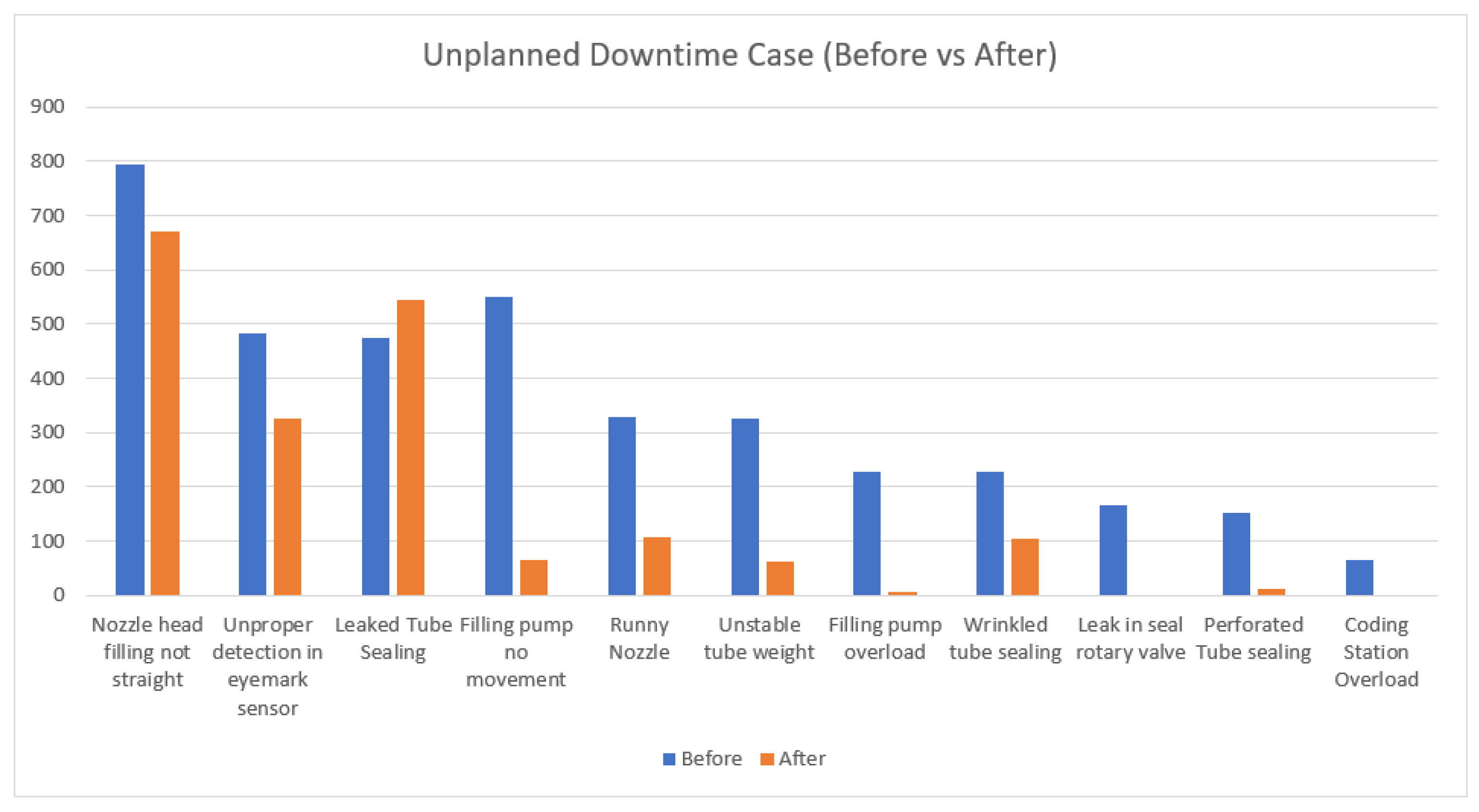
| Before (min) | Downtime Case | After (min) | Reduction (%) |
|---|---|---|---|
| 474 | Leaked tube sealing | 544 | +14.77% |
| 152 | Perforated tube sealing | 13 | −91.45% |
| 228 | Wrinkled tube sealing | 104 | −54.39% |
| 327 | Unstable tube weight | 62 | −81.04% |
| 425 | Filling pump no movement | 65 | −88.18% |
| 229 | Filling pump overload | 7 | −96.94% |
| 166 | Leak in seal rotary valve | 0 | −100.0% |
| 65 | Coding station overload | 0 | −100.0% |
| 329 | Runny Nozzle | 106 | −67.78% |
| 2520 | Total Monitored Downtime | 901 | −64.25% |
Publisher’s Note: MDPI stays neutral with regard to jurisdictional claims in published maps and institutional affiliations. |
© 2022 by the authors. Licensee MDPI, Basel, Switzerland. This article is an open access article distributed under the terms and conditions of the Creative Commons Attribution (CC BY) license (https://creativecommons.org/licenses/by/4.0/).
Share and Cite
Natanael, D.; Sutanto, H. Machine Learning Application Using Cost-Effective Components for Predictive Maintenance in Industry: A Tube Filling Machine Case Study. J. Manuf. Mater. Process. 2022, 6, 108. https://doi.org/10.3390/jmmp6050108
Natanael D, Sutanto H. Machine Learning Application Using Cost-Effective Components for Predictive Maintenance in Industry: A Tube Filling Machine Case Study. Journal of Manufacturing and Materials Processing. 2022; 6(5):108. https://doi.org/10.3390/jmmp6050108
Chicago/Turabian StyleNatanael, David, and Hadi Sutanto. 2022. "Machine Learning Application Using Cost-Effective Components for Predictive Maintenance in Industry: A Tube Filling Machine Case Study" Journal of Manufacturing and Materials Processing 6, no. 5: 108. https://doi.org/10.3390/jmmp6050108
APA StyleNatanael, D., & Sutanto, H. (2022). Machine Learning Application Using Cost-Effective Components for Predictive Maintenance in Industry: A Tube Filling Machine Case Study. Journal of Manufacturing and Materials Processing, 6(5), 108. https://doi.org/10.3390/jmmp6050108