
A Realistic Full-Scale 3D Modeling of Turning Using Coupled Smoothed Particle Hydrodynamics and Finite Element Method for Predicting Cutting Forces

 , ,
, ,
Abstract
:1. Introduction
2. Literature Review
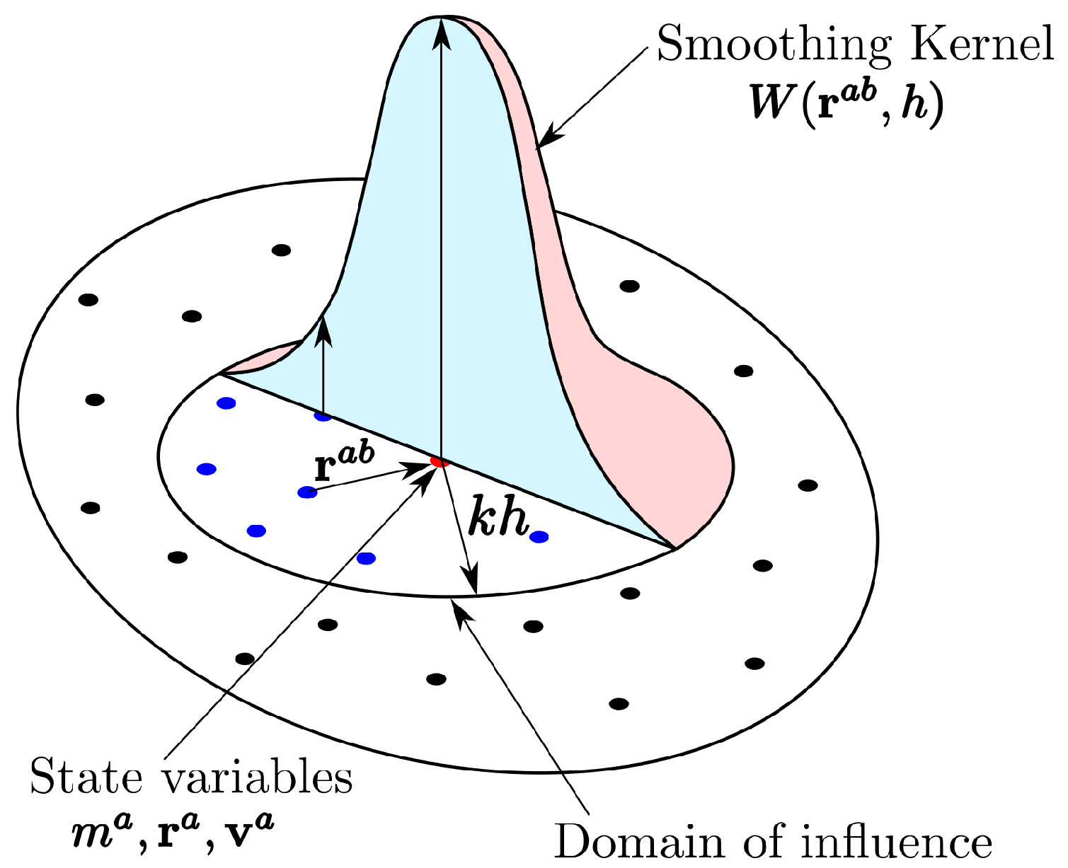
3. Smoothed Particle Hydrodynamics (SPH) Method
3.1. Discrete Form of Conservation Laws
3.2. Equation of State
3.3. Material Model
4. Machining Models
4.1. 2D Machining Model
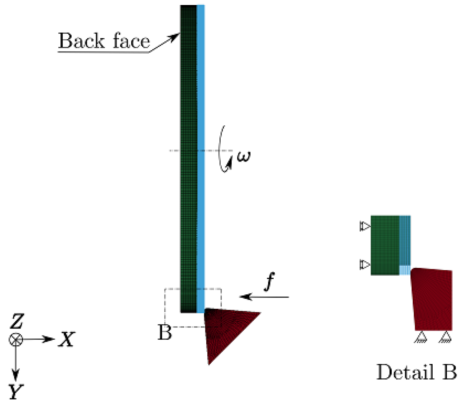
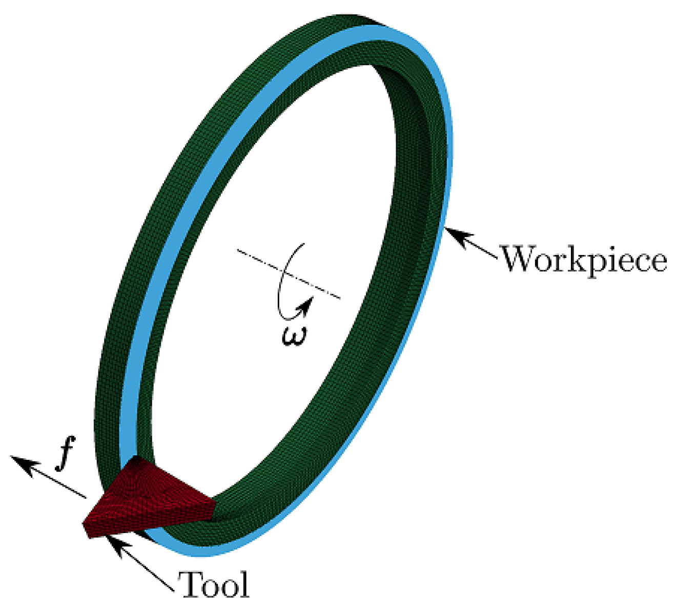
4.2. 3D Machining Model
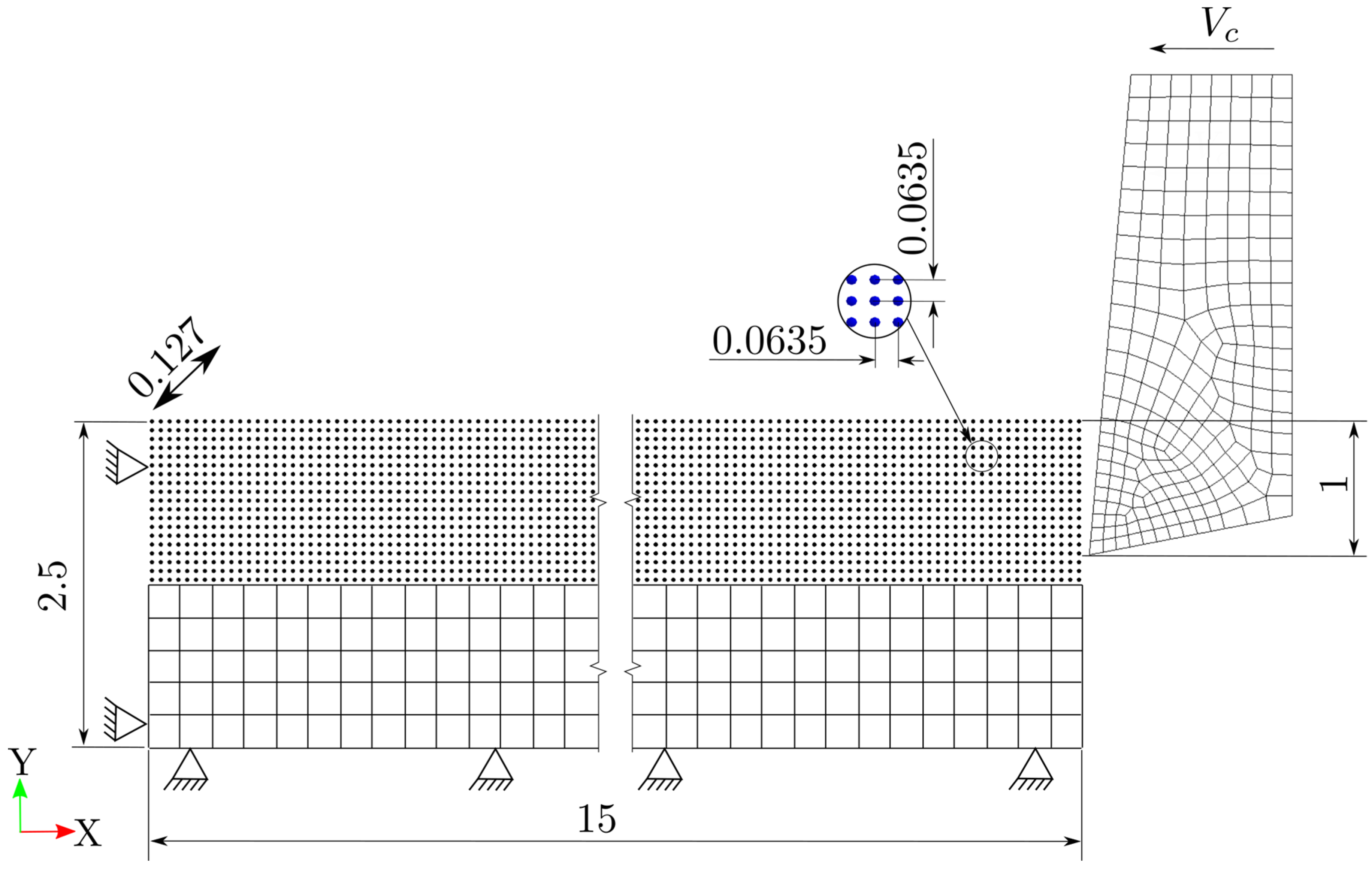
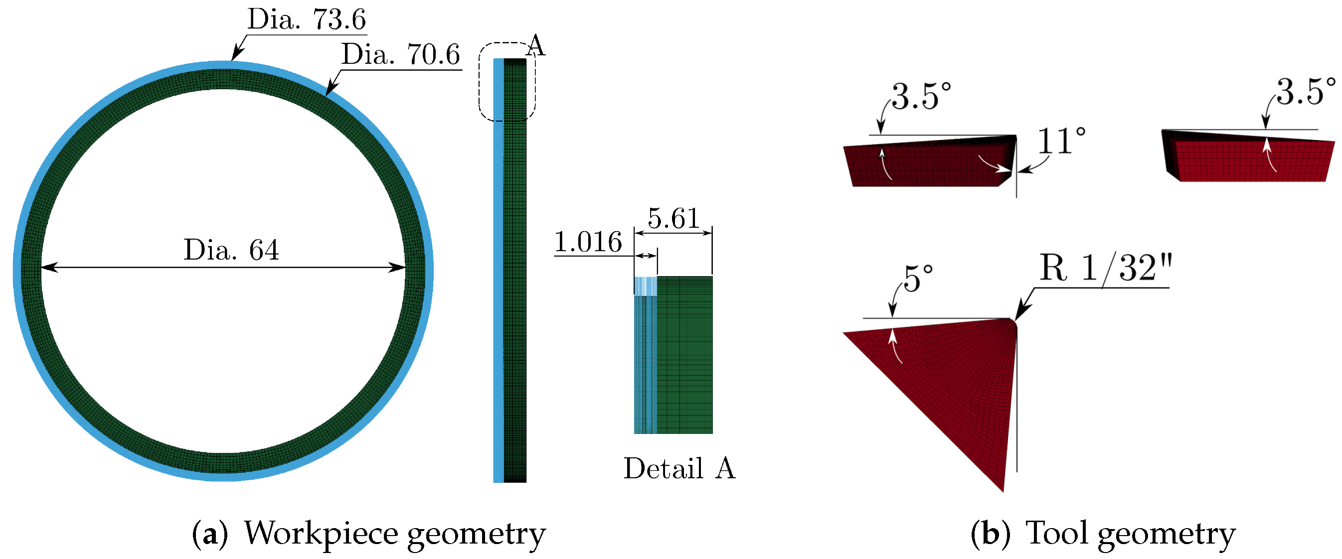
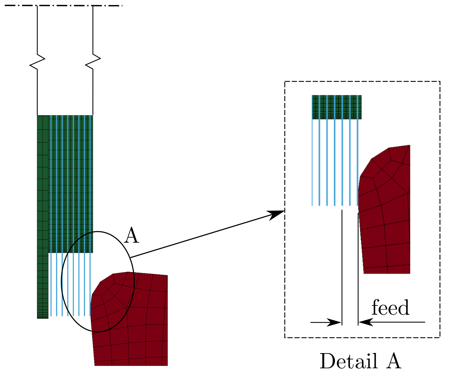
4.2.1. Geometry and Mesh
4.2.2. Material Properties
4.2.3. Boundary Conditions
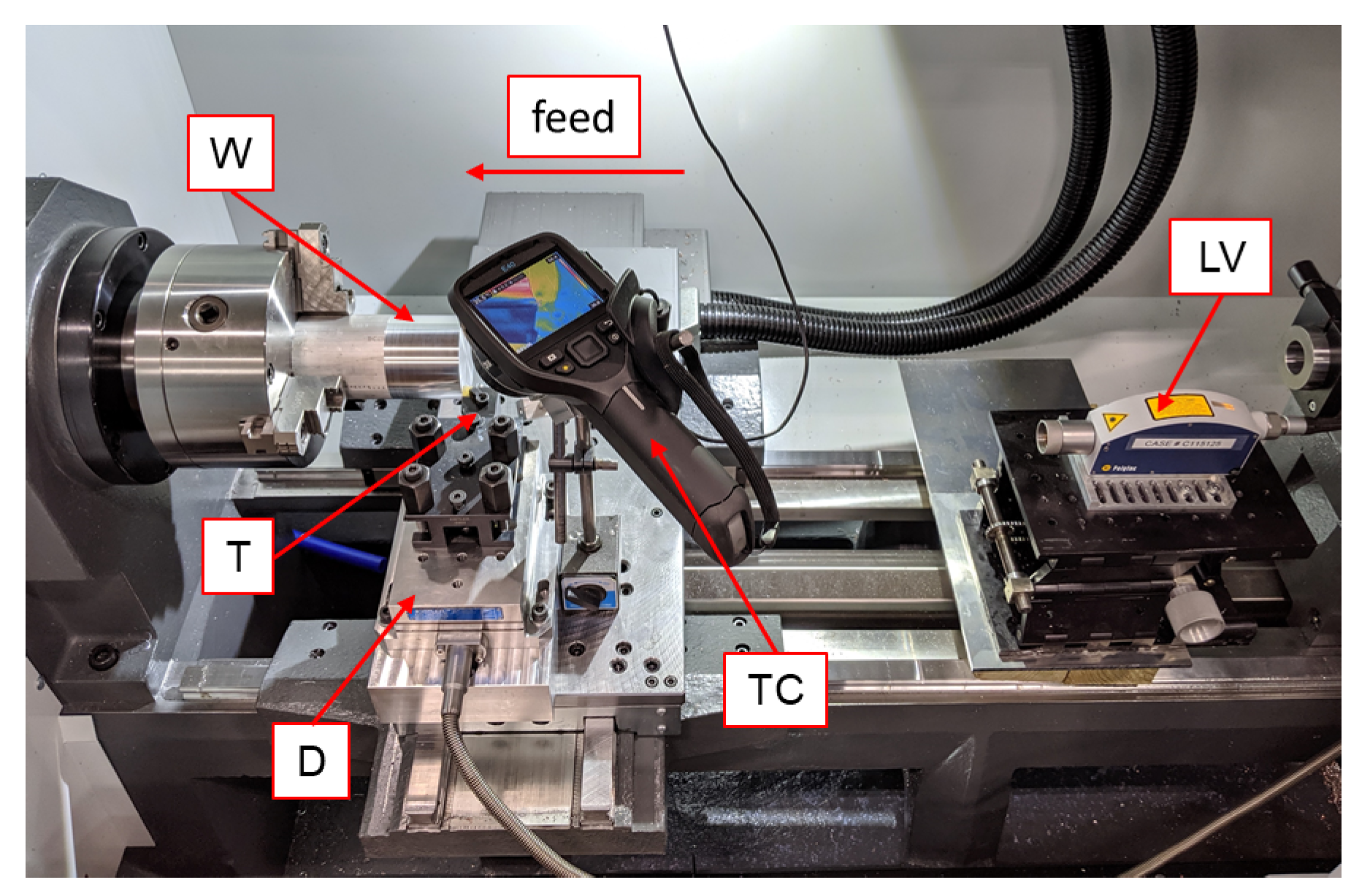
5. Machining Experimental Setup
6. Results
6.1. 2D Machining Simulation
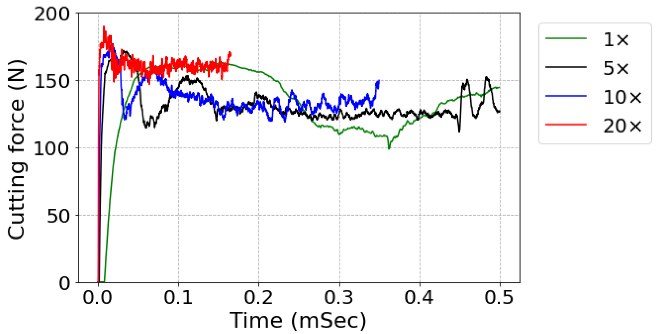
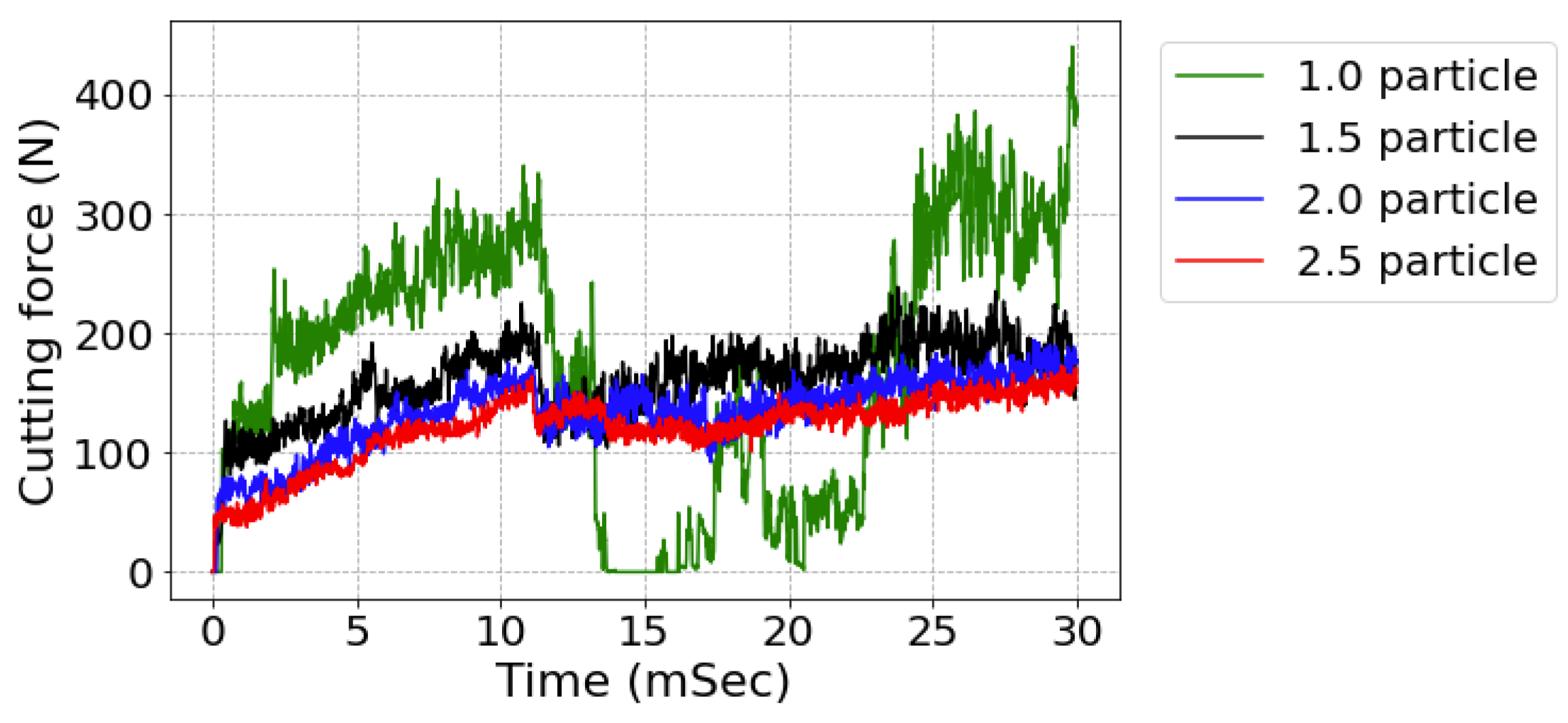
6.2. Convergence Study for 3D Machining Model
6.3. 3D Machining Simulation
7. Conclusions
- The simplified two-dimensional orthogonal, plane-strain model for the actual turning operation underpredicts the cutting force and the feed force. Additionally, the 2D model cannot predict the passive force. This necessitates the use of three-dimensional machining models.
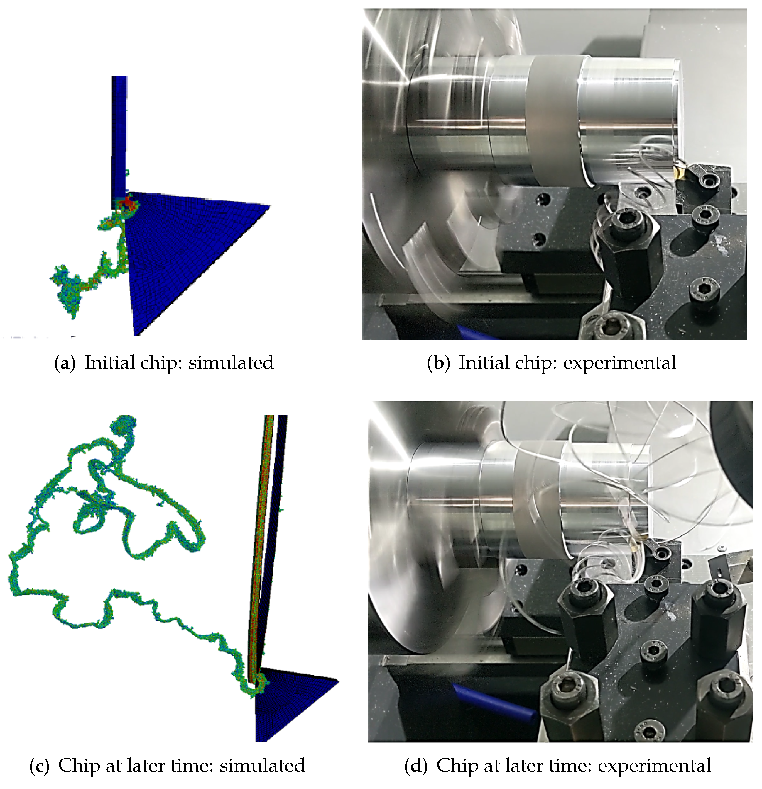
- The forces predicted by the three-dimensional model are considerably close to the experimental values. The chip morphology also correlates with experiments in terms of the direction of the chip movement and the “long” continuous chips observed while turning Al 6061.
- The value of friction coefficient between the tool and the workpiece has a significant influence on the simulated cutting forces, especially on the feed and passive force components. The feed cutting force governs the stability of the machining conditions. Hence, correct prediction of this force is important.
- The benefits of using the coupling of Smoothed Particle Hydrodynamics (SPH) and Finite Element Method (FEM) are successfully demonstrated in modelling of turning operation. The challenges associated with using the FE method such as mesh distortions and material separation modelling are easily handled by the SPH method. At the same time, the high computational times associated with SPH method are reduced with the use of the FE mesh in the low deformation zones.
Author Contributions
Funding
Data Availability Statement
Conflicts of Interest
References
- Sadeghifar, M.; Sedaghati, R.; Jomaa, W.; Songmene, V. A comprehensive review of finite element modeling of orthogonal machining process: Chip formation and surface integrity predictions. Int. J. Adv. Manuf. Technol. 2018, 96, 3747–3791. [Google Scholar] [CrossRef]
- Ivester, R.W.; Kennedy, M. Comparison of Machining Simulations for 1045 Steel to Experimental Measurements; Society of Manufacturing Engineers: Southfield, MI, USA, 2000. [Google Scholar]
- Arrazola, P.; Özel, T.; Umbrello, D.; Davies, M.; Jawahir, I. Recent advances in modelling of metal machining processes. CIRP Ann. 2013, 62, 695–718. [Google Scholar] [CrossRef]
- Zhang, B.; Bagchi, A. Finite element simulation of chip formation and comparison with machining experiment. J. Eng. Ind. 1994, 116, 289–297. [Google Scholar] [CrossRef]
- Mabrouki, T.; Girardin, F.; Asad, M.; Rigal, J.F. Numerical and experimental study of dry cutting for an aeronautic aluminium alloy (A2024-T351). Int. J. Mach. Tools Manuf. 2008, 48, 1187–1197. [Google Scholar] [CrossRef]
- Carroll, J.T., III; Strenkowski, J.S. Finite element models of orthogonal cutting with application to single point diamond turning. Int. J. Mech. Sci. 1988, 30, 899–920. [Google Scholar] [CrossRef]
- Movahhedy, M.; Gadala, M.; Altintas, Y. Simulation of the orthogonal metal cutting process using an arbitrary Lagrangian–Eulerian finite-element method. J. Mater. Process. Technol. 2000, 103, 267–275. [Google Scholar] [CrossRef]
- Chenot, J.L.; Bernacki, M.; Bouchard, P.O.; Fourment, L.; Hachem, E.; Perchat, E. Recent and future developments in finite element metal forming simulation. In Proceedings of the 11th International Conference on Technology of Plasticity, Nagoya, Japan, 19–24 October 2014; pp. 265–293. [Google Scholar]
- Limido, J.; Espinosa, C.; Salaün, M.; Lacome, J.L. SPH method applied to high speed cutting modelling. Int. J. Mech. Sci. 2007, 49, 898–908. [Google Scholar] [CrossRef] [Green Version]
- Villumsen, M.F.; Fauerholdt, T.G. Simulation of Metal Cutting Using Smooth Particle Hydrodynamics; LS-DYNA Anwenderforum C-III 17; DYNAmore FEM Ingenieurdienstleistungen GmbH: Stuttgart, Germany, 2008. [Google Scholar]
- Avachat, C.S.; Cherukuri, H.P. A Parametric Study of the Modeling of Orthogonal Machining Using the Smoothed Particle Hydrodynamics Method. In American Society of Mechanical Engineers Digital Collection, Proceedings of the ASME 2015 International Mechanical Engineering Congress and Exposition, Houston, TX, USA, 13–19 November 2015; American Society of Mechanical Engineers: New York, NY, USA, 2015. [Google Scholar]
- Xi, Y.; Bermingham, M.; Wang, G.; Dargusch, M. SPH/FE modeling of cutting force and chip formation during thermally assisted machining of Ti6Al4V alloy. Comput. Mater. Sci. 2014, 84, 188–197. [Google Scholar] [CrossRef]
- Song, H.; Pan, P.; Ren, G.; Yang, Z.; Dan, J.; Li, J.; Xiao, J.; Xu, J. SPH/FEM modeling for laser-assisted machining of fused silica. Int. J. Adv. Manuf. Technol. 2020, 106, 2049–2064. [Google Scholar] [CrossRef]
- Mane, S.; Joshi, S.S.; Karagadde, S.; Kapoor, S.G. Modeling of variable friction and heat partition ratio at the chip-tool interface during orthogonal cutting of Ti-6Al-4V. J. Manuf. Process. 2020, 55, 254–267. [Google Scholar] [CrossRef]
- Laakso, S.V.; Agmell, M.; Ståhl, J.E. The mystery of missing feed force-The effect of friction models, flank wear and ploughing on feed force in metal cutting simulations. J. Manuf. Process. 2018, 33, 268–277. [Google Scholar] [CrossRef]
- Calamaz, M.; Coupard, D.; Girot, F. A new material model for 2D numerical simulation of serrated chip formation when machining titanium alloy Ti–6Al–4V. Int. J. Mach. Tools Manuf. 2008, 48, 275–288. [Google Scholar] [CrossRef] [Green Version]
- Childs, T.; Rahmad, R. Modifying strain-hardening of carbon steels for improved finite element simulation of orthogonal machining. Proc. Inst. Mech. Eng. Part B J. Eng. Manuf. 2010, 224, 721–732. [Google Scholar] [CrossRef]
- Llanos, I.; Villar, J.; Urresti, I.; Arrazola, P. Finite element modeling of oblique machining using an arbitrary Lagrangian–Eulerian formulation. Mach. Sci. Technol. 2009, 13, 385–406. [Google Scholar] [CrossRef]
- Olleak, A.; Özel, T. 3D finite element modeling based investigations of micro-textured tool designs in machining titanium alloy Ti-6Al-4V. Procedia Manuf. 2017, 10, 536–545. [Google Scholar] [CrossRef]
- Özel, T.; Llanos, I.; Soriano, J.; Arrazola, P.J. 3D finite element modelling of chip formation process for machining Inconel 718: Comparison of FE software predictions. Mach. Sci. Technol. 2011, 15, 21–46. [Google Scholar] [CrossRef]
- Shi, B.; Elsayed, A.; Damir, A.; Attia, H.; M’Saoubi, R. A hybrid modeling approach for characterization and simulation of cryogenic machining of Ti–6Al–4V alloy. J. Manuf. Sci. Eng. 2019, 141. [Google Scholar] [CrossRef] [Green Version]
- Liu, G.; Huang, C.; Su, R.; Özel, T.; Liu, Y.; Xu, L. 3D FEM simulation of the turning process of stainless steel 17-4PH with differently texturized cutting tools. Int. J. Mech. Sci. 2019, 155, 417–429. [Google Scholar] [CrossRef]
- Kyratsis, P.; Tzotzis, A.; Markopoulos, A.; Tapoglou, N. Cad-based 3d-fe modelling of aisi-d3 turning with ceramic tooling. Machines 2021, 9, 4. [Google Scholar] [CrossRef]
- Gingold, R.A.; Monaghan, J.J. Smoothed particle hydrodynamics: Theory and application to non-spherical stars. Mon. Not. R. Astron. Soc. 1977, 181, 375–389. [Google Scholar] [CrossRef]
- Lucy, L.B. A numerical approach to the testing of the fission hypothesis. Astron. J. 1977, 82, 1013–1024. [Google Scholar] [CrossRef]
- Liu, G.; Liu, M.; Li, S. Smoothed particle hydrodynamics—A meshfree method. Comput. Mech. 2004, 33, 491. [Google Scholar] [CrossRef]
- Feng, L.; Liu, G.; Li, Z.; Dong, X.; Du, M. Study on the effects of abrasive particle shape on the cutting performance of Ti-6Al-4V materials based on the SPH method. Int. J. Adv. Manuf. Technol. 2019, 101, 3167–3182. [Google Scholar] [CrossRef]
- Steinberg, D. Equation of State and Strength Properties of Selected Materials; Lawrence Livermore National Laboratory Livermore: Livermore, CA, USA, 1996. [Google Scholar]
- Johnson, G.; Holmquist, T. Test Data and Computational Strength and Fracture Model Constants for 23 Materials Subjected to Large Strains, High Strain Rates, and High Temperatures; Report No. LA-11463-MS; Los Alamos National Laboratory: Los Alamos, NM, USA, 1989. [Google Scholar]
- Jo, H. LS-DYNA Theory Manual; LSTC: Livermore, CA, USA, 2006. [Google Scholar]
- Ojal, N.; Cherukuri, H.P.; Schmitz, T.L.; Jaycox, A.W. A Comparison of Smoothed Particle Hydrodynamics (SPH) and Coupled SPH-FEM Methods for Modeling Machining. In ASME International Mechanical Engineering Congress and Exposition; American Society of Mechanical Engineers: New York, NY, USA, 2020; Volume 84485, p. V02AT02A036. [Google Scholar]
- ASTM. Standard ASTM B211:2012; Standard Specification for Aluminum and Aluminum-Alloy Rolled or Cold Finished Bar, Rod, and Wire. ASTM International: West Conshohocken, PA, USA, 2012. [CrossRef]
- ASM Material Data Sheet. ASM Aerospace Specification Metals, Inc. 2020. Available online: http://asm.matweb.com/search/SpecificMaterial.asp?bassnum=MA6061T6 (accessed on 11 December 2020).
- Schwer, L.E.; Windsor, C. Aluminum plate perforation: A comparative case study using Lagrange with erosion, multi-material ALE, and smooth particle hydrodynamics. In Proceedings of the Seventh European LS-DYNA Conference, Stuttgart, Germany, 14–15 June 2009; Volume 10. [Google Scholar]
- Karandikar, J.M.; Schmitz, T.L.; Abbas, A.E. Spindle speed selection for tool life testing using Bayesian inference. J. Manuf. Syst. 2012, 31, 403–411. [Google Scholar] [CrossRef]
- Tyler, C.T.; Schmitz, T.L. Examining the effects of cooling/lubricating conditions on tool wear in milling Hastelloy X. Proc. NAMRI/SME 2014, 42, 435–442. [Google Scholar]
- ISO. Standard ISO 3685:1993; Tool-Life Testing with Single-Point Turning Tools. International Organization for Standardization: Geneva, Switzerland, 1993.
- Stenberg, N.; Delić, A.; Björk, T. Using the SPH method to easier predict wear in machining. Procedia CIRP 2017, 58, 317–322. [Google Scholar] [CrossRef]
- Espinosa, C.; Lacome, J.L.; Limido, J.; Salaün, M.; Mabru, C.; Chieragatti, R. Modelling High Speed Machining with the SPH Method. In Proceedings of the 10th International LS-DYNA® Users Conference, Dearborn, MI, USA, 8–10 June 2008. [Google Scholar]
- Umbrello, D.; M’saoubi, R.; Outeiro, J. The influence of Johnson–Cook material constants on finite element simulation of machining of AISI 316L steel. Int. J. Mach. Tools Manuf. 2007, 47, 462–470. [Google Scholar] [CrossRef]
- Storchak, M.; Rupp, P.; Möhring, H.C.; Stehle, T. Determination of Johnson–Cook Constitutive Parameters for Cutting Simulations. Metals 2019, 9, 473. [Google Scholar] [CrossRef] [Green Version]
- Özel, T. The influence of friction models on finite element simulations of machining. Int. J. Mach. Tools Manuf. 2006, 46, 518–530. [Google Scholar] [CrossRef]
- Madaj, M.; Píška, M. On the SPH orthogonal cutting simulation of A2024-T351 alloy. Procedia CIRP 2013, 8, 152–157. [Google Scholar] [CrossRef] [Green Version]
- Merchant, M.E. Basic mechanics of the metal-cutting process. J. Appl. Mech. 1944, 11, A168–A175. [Google Scholar] [CrossRef]


| Element | Si | Fe | Cu | Mn | Mg | Cr | Zn | Sn | Al |
|---|---|---|---|---|---|---|---|---|---|
| Content % | 0.4–0.8 | 0.7 | 0.15–0.4 | 0.15 | 0.8–1.2 | 0.04–0.35 | 0.25 | 0.15 | remainder |
| Property | Workpiece | Tool |
|---|---|---|
| Density, (Kg/m3) | 2700 | 11,900 |
| Young’s Modulus, E (GPa) | 68.9 | 534 |
| Poisson’s ratio, | 0.33 | 0.22 |
| Specific heat, Cp (J/Kg K−1) | 896 | - |
| Tmelt, (K) | 855 | - |
| Troom, (K) | 300 | 300 |
| Parameter | A (MPa) | B (MPa) | n | C | m |
|---|---|---|---|---|---|
| Value | 324 | 114 | 0.42 | 0.002 | 1.34 |
| Parameter | |||||
| Value | −0.77 | 1.45 | −0.47 | 0 | 1.6 |
| Experimental (N) | Simulated (N) | |
|---|---|---|
| Feed Force () | 100 | - |
| Passive Force () | 65 | 19 |
| Cutting Force () | 235 | 120 |
| Total Force (F) | 264 | 121 |
| Particle/Feed | Number of Particles | Run Time | Processors |
|---|---|---|---|
| 1.0 | 43,708 | 7.25 h | 144 |
| 1.5 | 101,952 | 24.50 h | 144 |
| 2.0 | 192,280 | 64.75 h | 144 |
| 2.5 | 323,232 | 183.50 h | 144 |
| Experimental (N) | Simulated (N) | |
|---|---|---|
| Feed Force () | 100 | 106 |
| Passive Force () | 65 | 60 |
| Cutting Force () | 235 | 180 |
| Total Force (F) | 264 | 219 |
| Experiment (N) | Sim. (N) | Sim. (N) | |
|---|---|---|---|
| Feed Force () | 100 | 45 | 106 |
| Passive Force () | 65 | 10 | 60 |
| Cutting Force () | 235 | 210 | 180 |
| Total Force (F) | 264 | 215 | 219 |
Publisher’s Note: MDPI stays neutral with regard to jurisdictional claims in published maps and institutional affiliations. |
© 2022 by the authors. Licensee MDPI, Basel, Switzerland. This article is an open access article distributed under the terms and conditions of the Creative Commons Attribution (CC BY) license (https://creativecommons.org/licenses/by/4.0/).
Share and Cite
Ojal, N.; Copenhaver, R.; Cherukuri, H.P.; Schmitz, T.L.; Devlugt, K.T.; Jaycox, A.W. A Realistic Full-Scale 3D Modeling of Turning Using Coupled Smoothed Particle Hydrodynamics and Finite Element Method for Predicting Cutting Forces. J. Manuf. Mater. Process. 2022, 6, 33. https://doi.org/10.3390/jmmp6020033
Ojal N, Copenhaver R, Cherukuri HP, Schmitz TL, Devlugt KT, Jaycox AW. A Realistic Full-Scale 3D Modeling of Turning Using Coupled Smoothed Particle Hydrodynamics and Finite Element Method for Predicting Cutting Forces. Journal of Manufacturing and Materials Processing. 2022; 6(2):33. https://doi.org/10.3390/jmmp6020033
Chicago/Turabian StyleOjal, Nishant, Ryan Copenhaver, Harish P. Cherukuri, Tony L. Schmitz, Kyle T. Devlugt, and Adam W. Jaycox. 2022. "A Realistic Full-Scale 3D Modeling of Turning Using Coupled Smoothed Particle Hydrodynamics and Finite Element Method for Predicting Cutting Forces" Journal of Manufacturing and Materials Processing 6, no. 2: 33. https://doi.org/10.3390/jmmp6020033
APA StyleOjal, N., Copenhaver, R., Cherukuri, H. P., Schmitz, T. L., Devlugt, K. T., & Jaycox, A. W. (2022). A Realistic Full-Scale 3D Modeling of Turning Using Coupled Smoothed Particle Hydrodynamics and Finite Element Method for Predicting Cutting Forces. Journal of Manufacturing and Materials Processing, 6(2), 33. https://doi.org/10.3390/jmmp6020033