
Modelling the Heating Process in the Transient and Steady State of an In Situ Tape-Laying Machine Head

 ,
,  ,
,  and
and
Abstract
:1. Introduction and Related Works
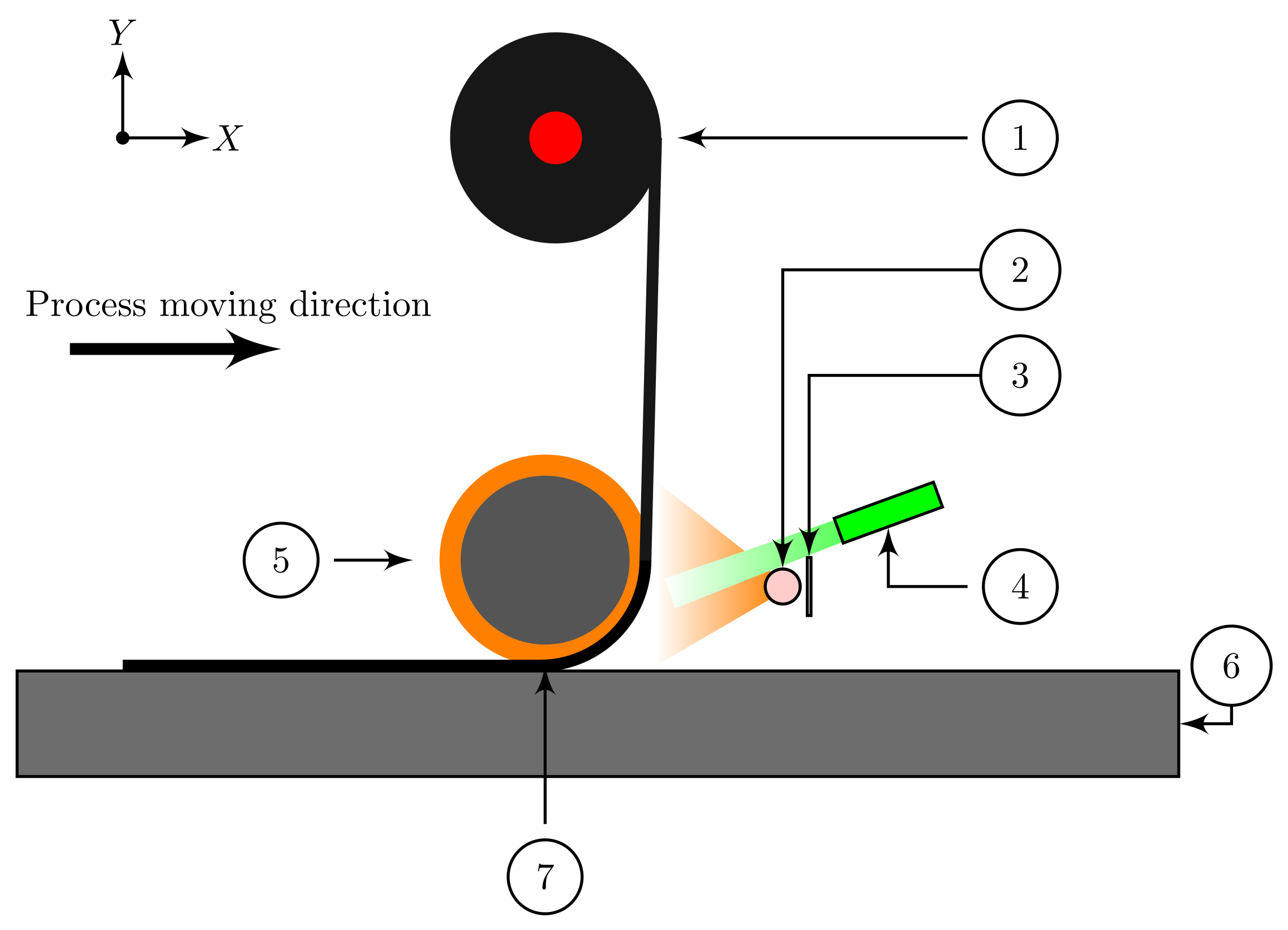
2. The ATL Machine Head
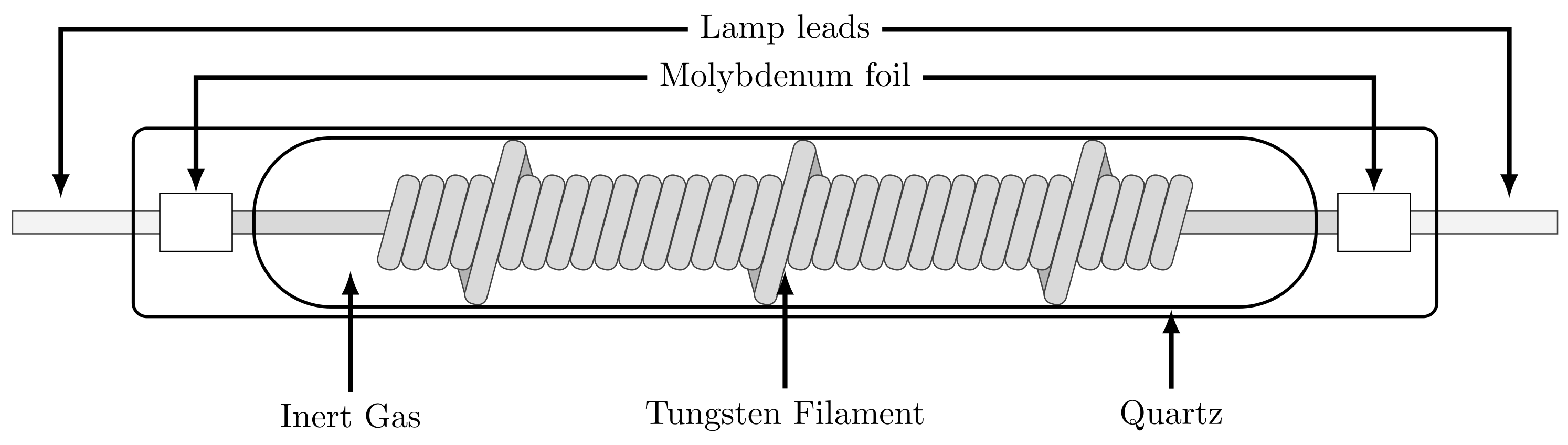
2.1. Infrared Heating Element
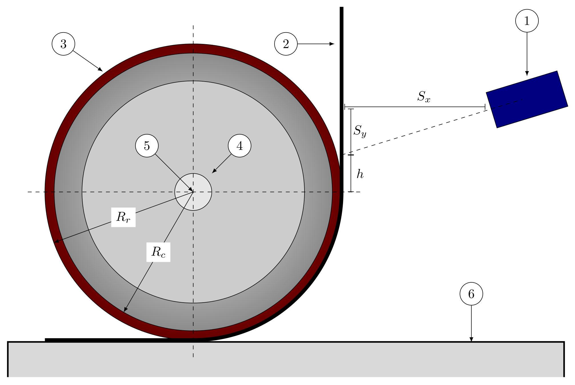
2.2. Compaction Roll
2.3. Material Feeder
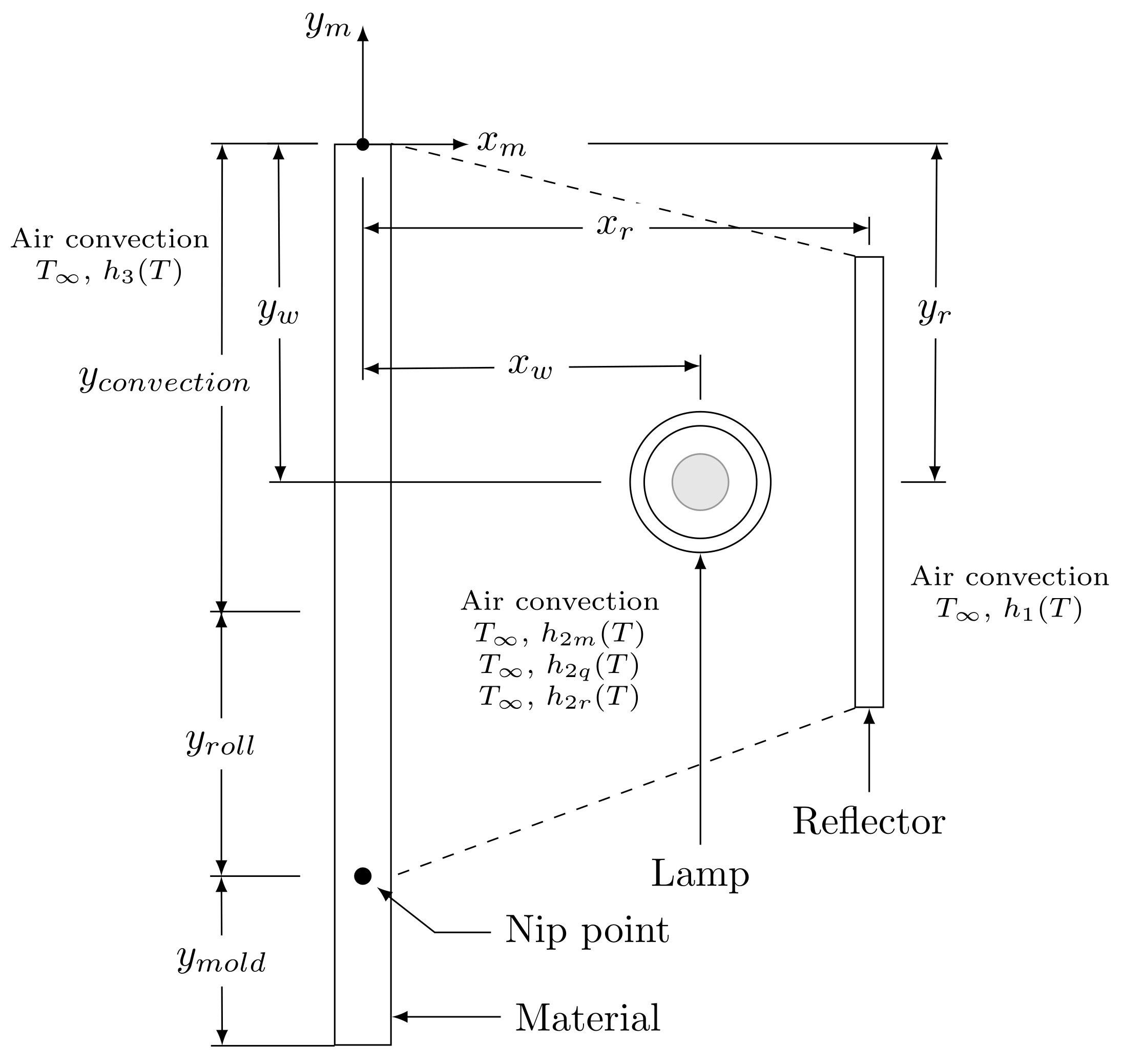
3. 1.5D Mathematical Model for the ATL Heating Process
3.1. Heater
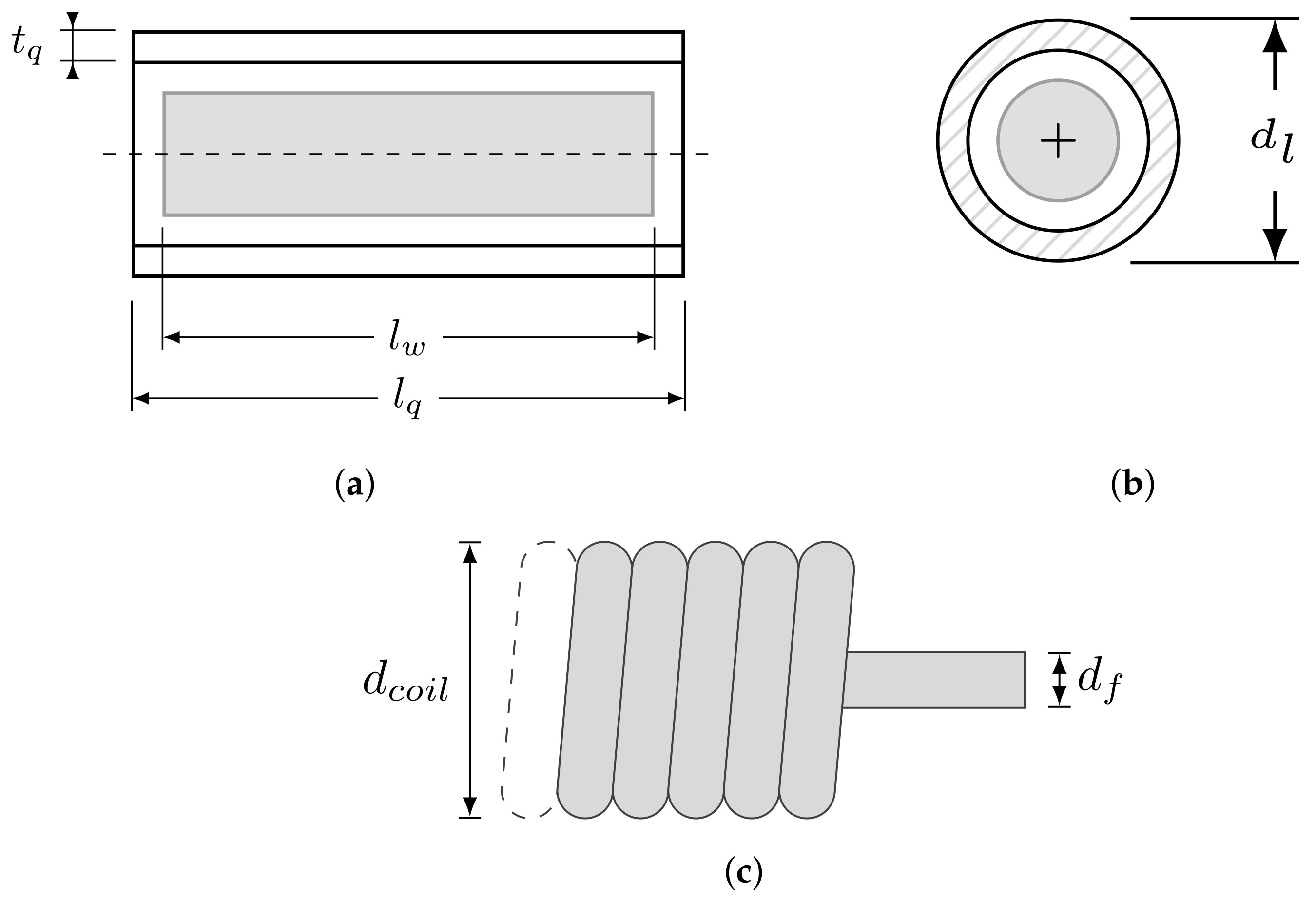
3.1.1. Tungsten Filament
- : Filament mass, kg.
- : Filament temperature, K.
- : Filament specific heat (temperature dependent), .
- : Electric power, W.
- : Radiation heat, W.
- : Conduction heat, W.
3.1.2. Neon
- : Conduction heat, W.
- : Neon conductivity (temperature dependent), .
- : Neon mean temperature , K.
- : Quartz lamp temperature, K.
- : Lamp diameter, m.
- : Filament coil diameter, m.
- : Lamp length, m.
3.1.3. Quartz Glass Envelope
- : Quartz cylinder mass, kg.
- : Quartz specific heat, .
- : Incoming radiation heat, W.
- : Outgoing radiation heat, W.
- : Conduction heat, W.
- : Convection coefficient, .
- : Quartz surface area, .
- : Air Temperature inside the radiation cavity, K
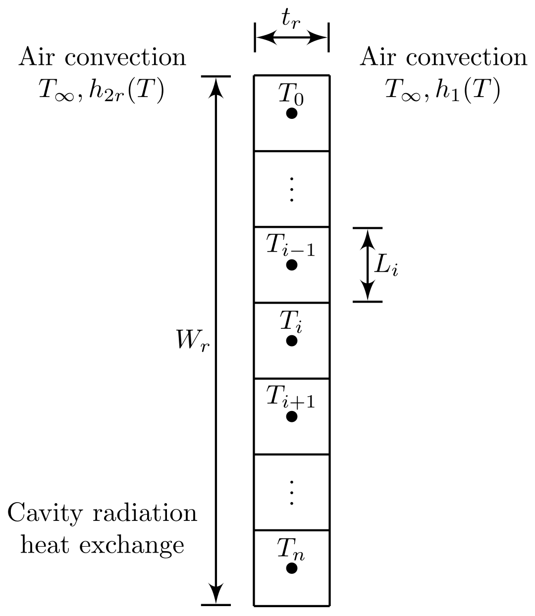
3.2. Reflector
- : Reflector material density, .
- : Reflector temperature, K.
- : Reflector specific heat (temperature dependent), .
- : Reflector conductivity (temperature dependent), .
- : Radiation heat, .
- : Convection heat .
- r: Reflector cell number 0,1,...,n.
- : Length of reflector cell, m.
- : Reflector thickness, m.
- : Air temperature, K.
- : External convection coefficient, .
- : Internal convection coefficient, .
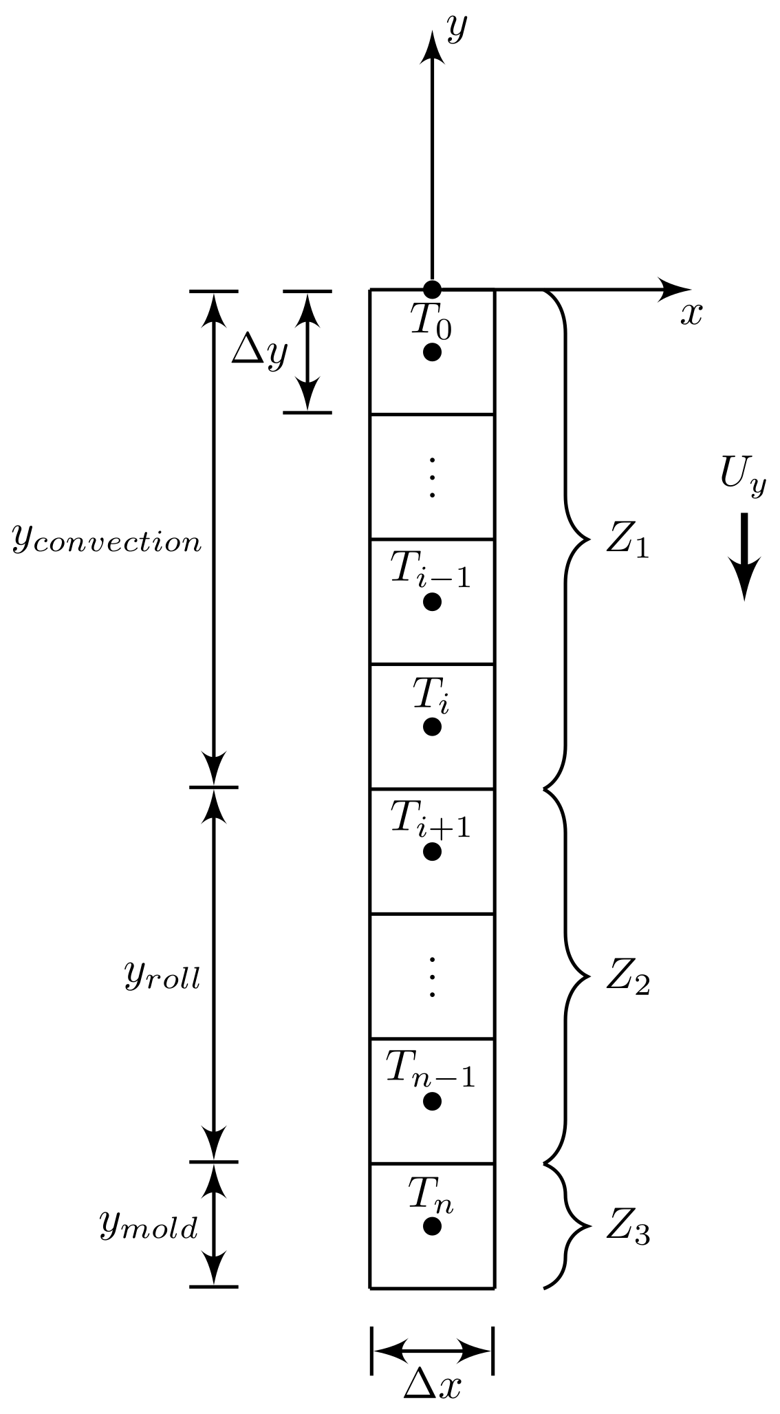
3.3. Material
- : Composite material density, .
- : Material Temperature, K.
- : Composite specific heat (temperature dependent), .
- : Composite conductivity (temperature dependent), .
- : Radiation heat, .
- : Convection heat, .
- : Conduction heat, .
- m: Material cell number 0, 1,..., n.
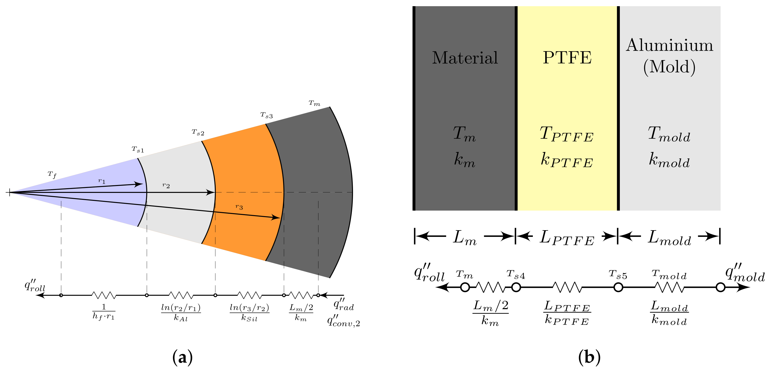
- : Composite wall resistance for heat conduction between the mold and the material, .
- : Composite wall resistance for heat conduction between compaction roll and the material, .
- : Net radiation from the surfaces involved in the heat exchange process, .
- : Convection coefficient for the material surface facing the heating element, .
3.4. Compaction Roll and Mold
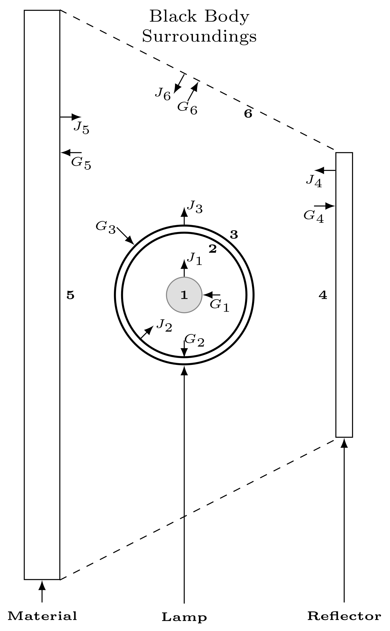
3.5. Radiation
- : Wavelength, m.
- T: Absolute temperature of the black body, K.
- h: Universal Planck constant, .
- : Boltzmann constant, .
- : Speed of light in vacuum, .
3.5.1. Radiative Fluxes
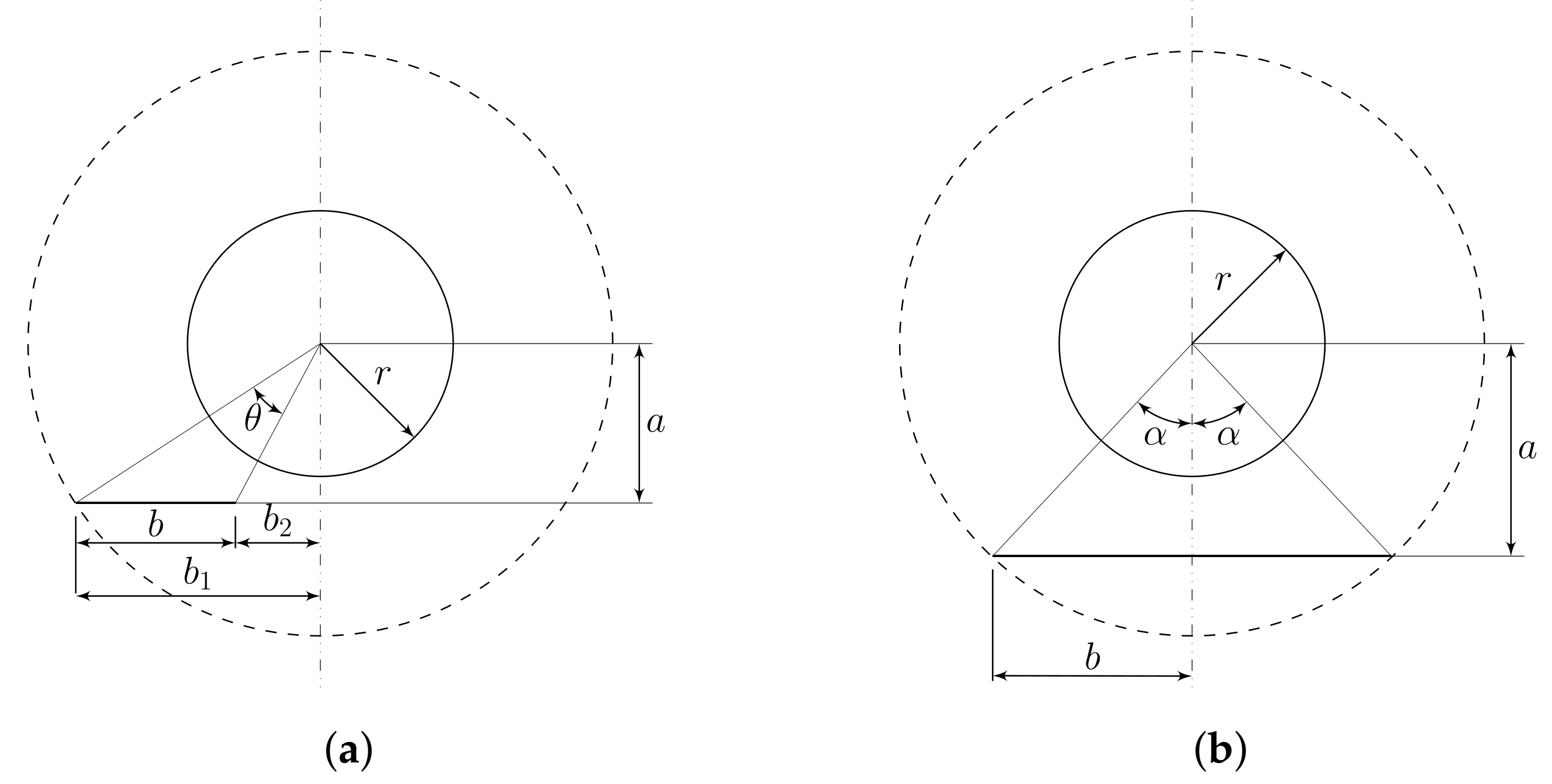
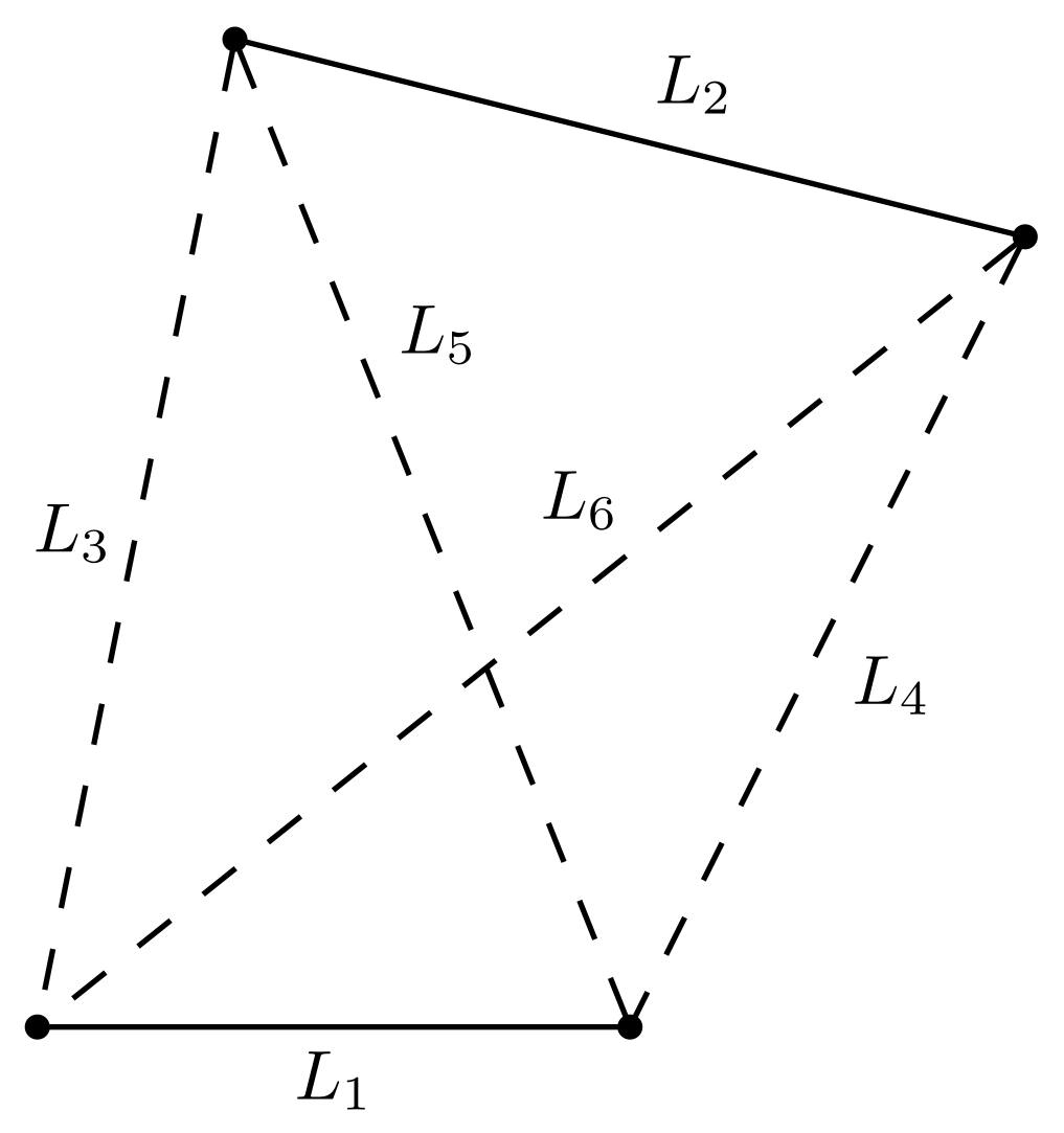
3.5.2. View Factors
4. Properties
4.1. Thermal Properties
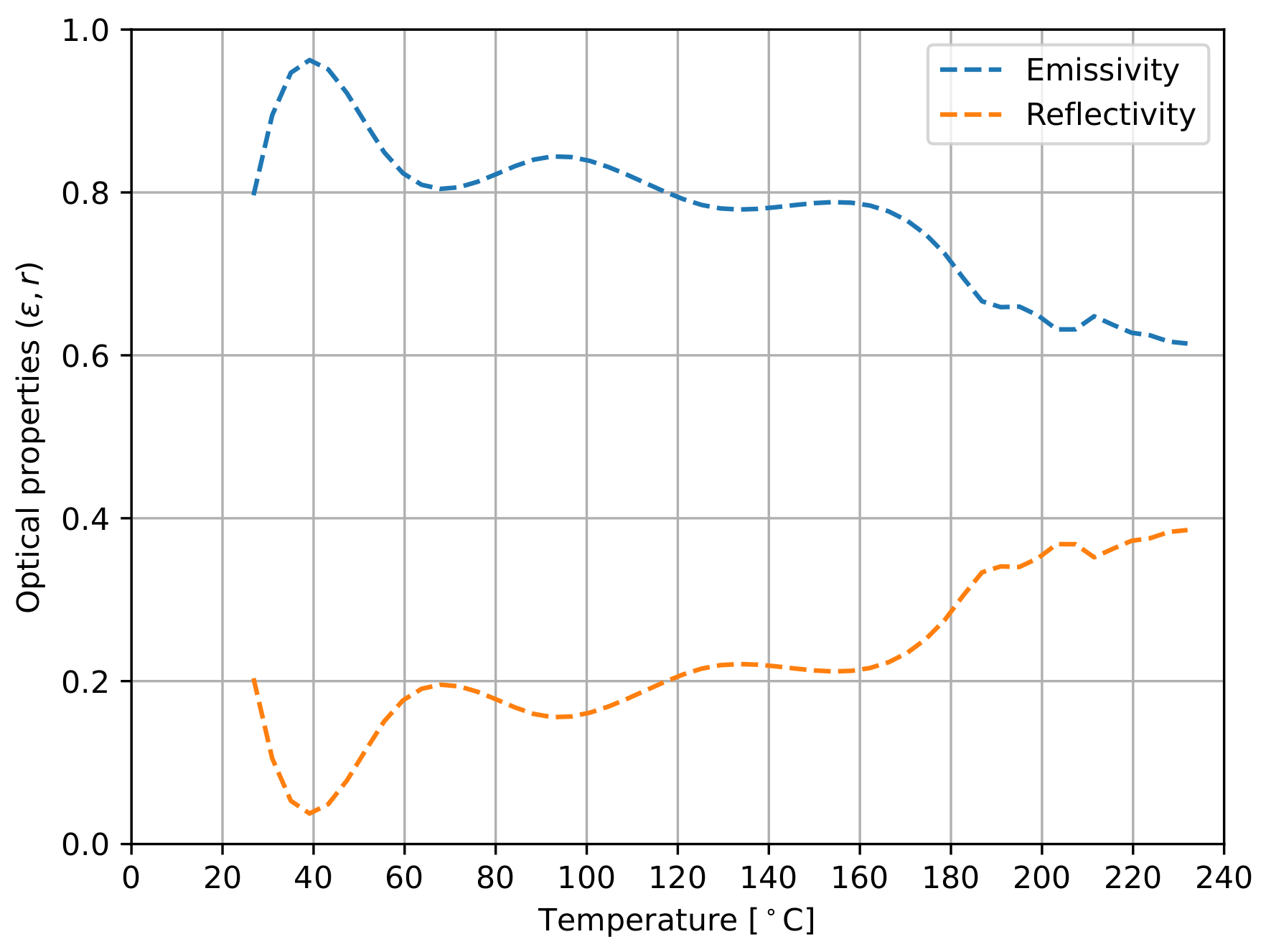
4.2. Optical Properties
- : relative material i permitivity.
- : vacuum permitivity .
4.3. Convection Coefficients
5. Materials and Methods
5.1. Material Description
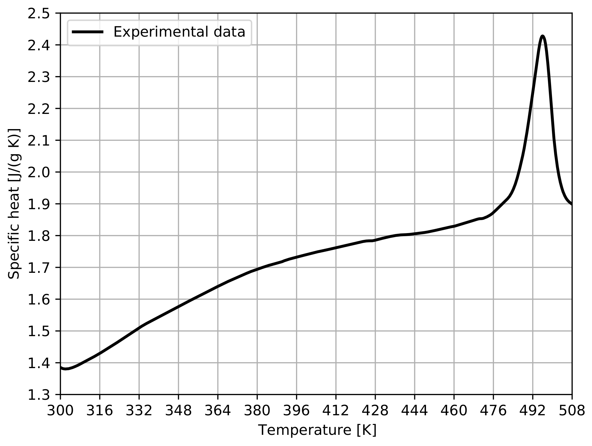
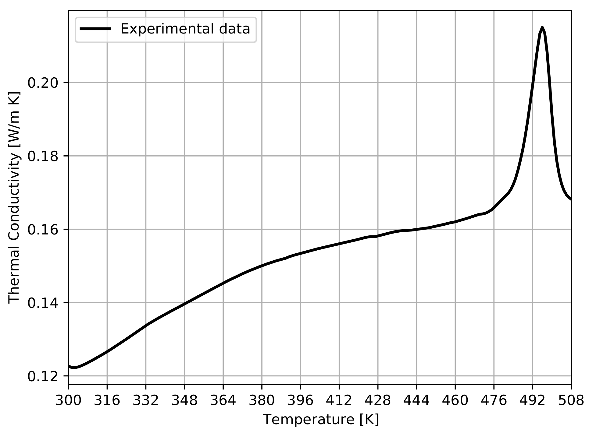
5.1.1. Thermal Properties
5.1.2. Optical Properties
5.2. Methods
5.2.1. Time Integration Scheme
- Step 1.
- For the given trial temperature.
- Step 2.
- Evaluate all material properties at the trial temperature.
- Step 3.
- Solve the radiation heat flux system for the trial temperature.
- Step 4.
- Evaluate the ODE system array with the temperature derivatives.
5.2.2. Convergence Analysis
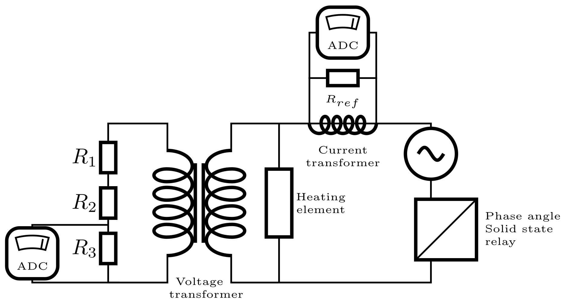
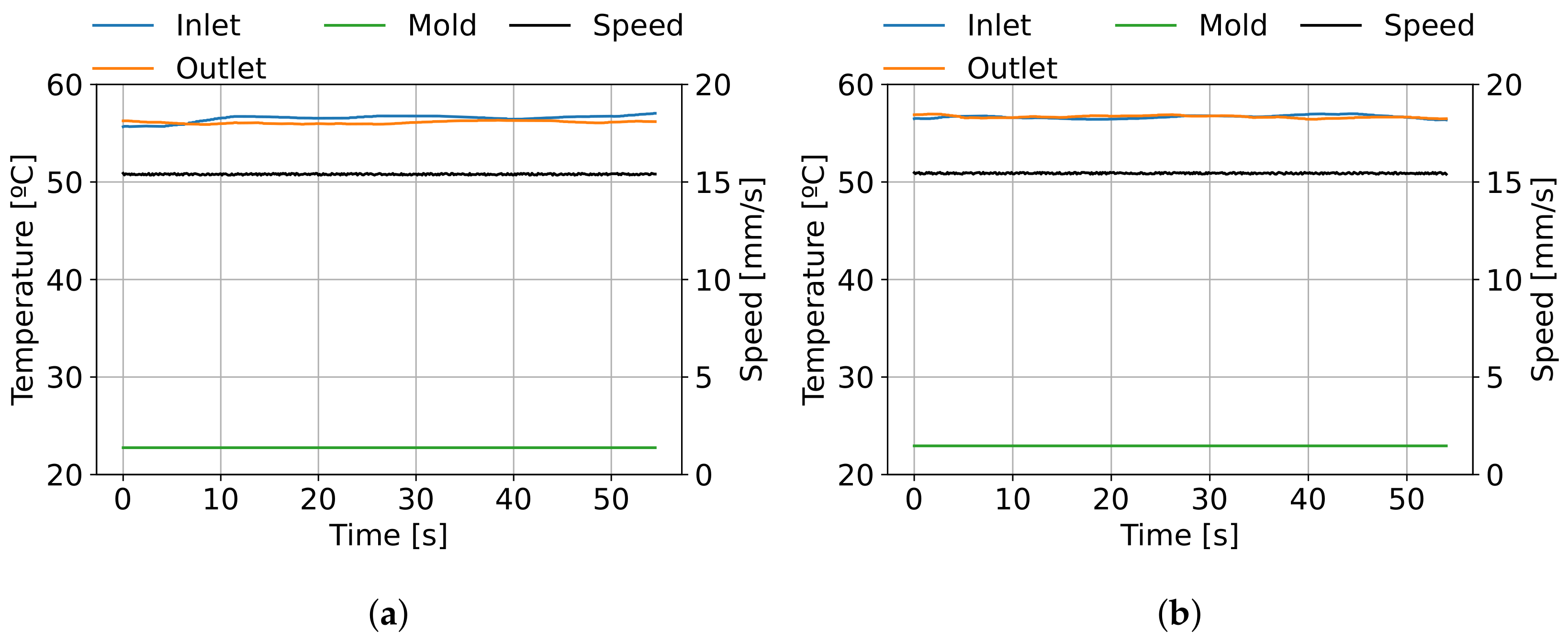
5.2.3. Measures and Instrumentation
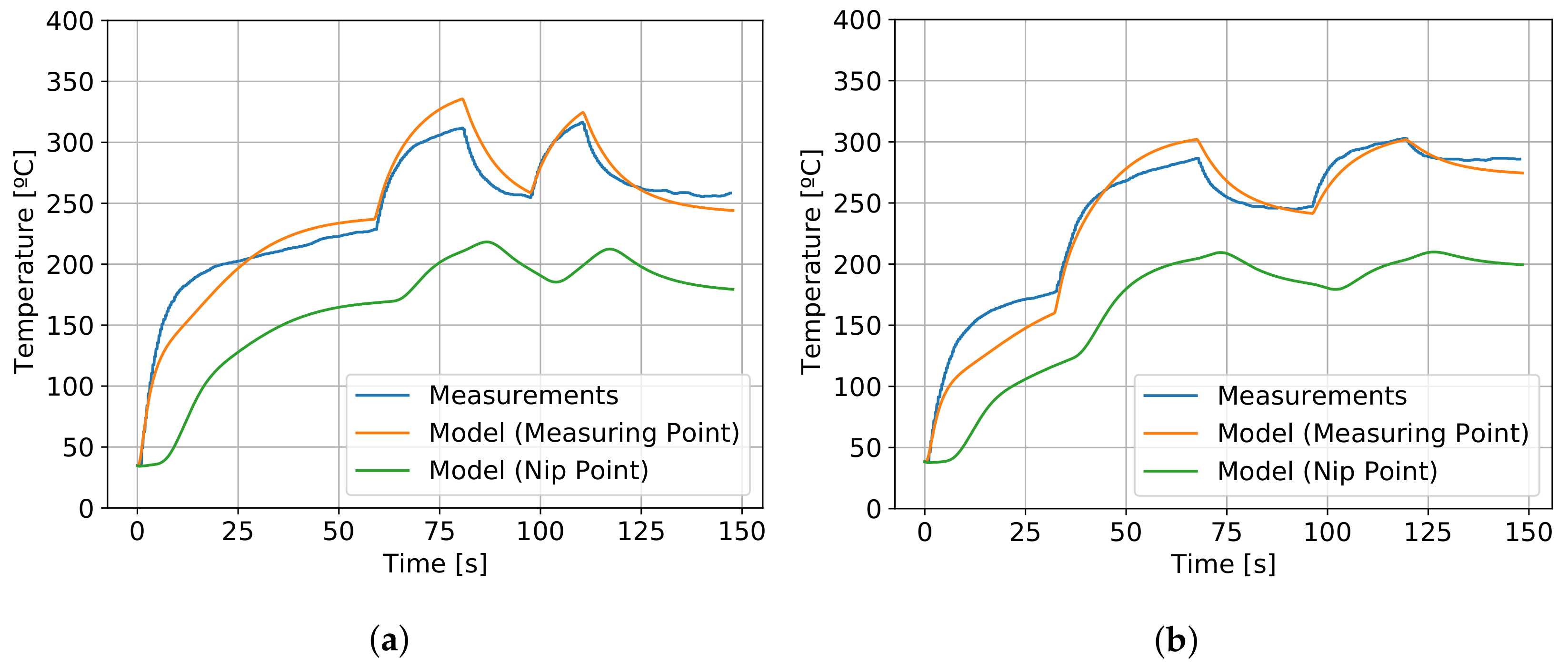
5.2.4. Model Validation
6. Results
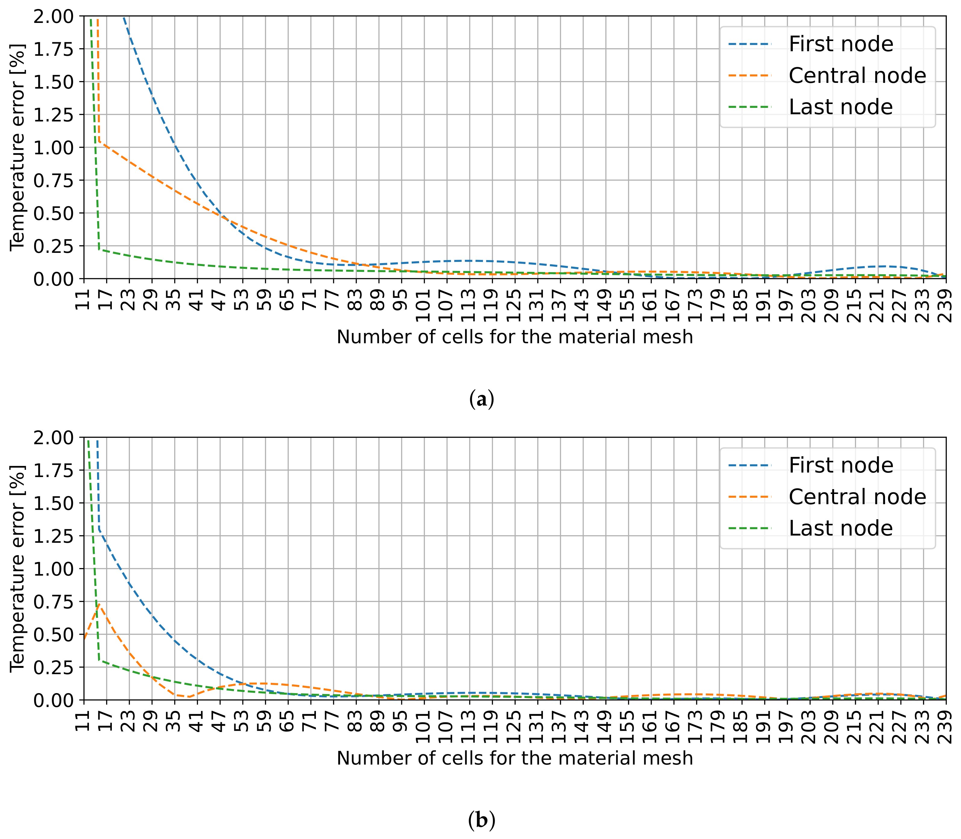
6.1. Mesh Convergence
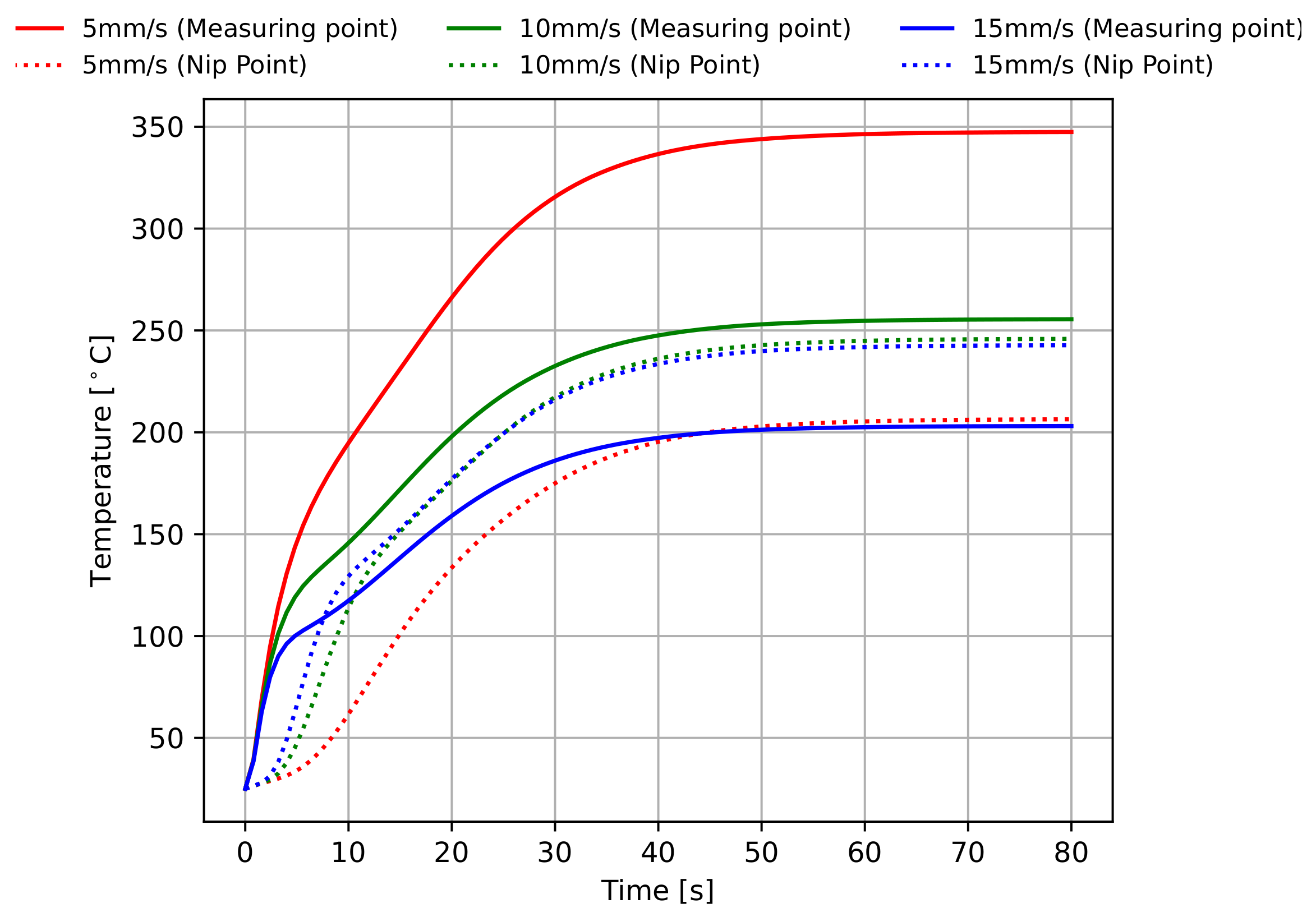
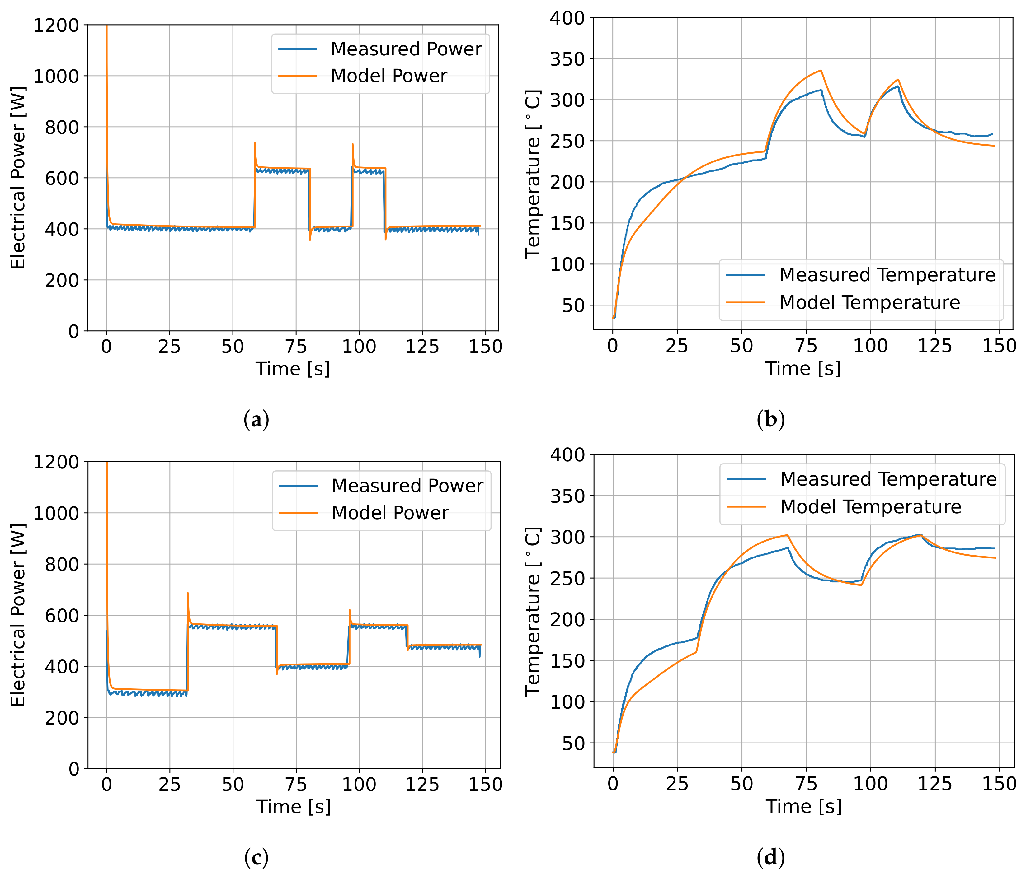
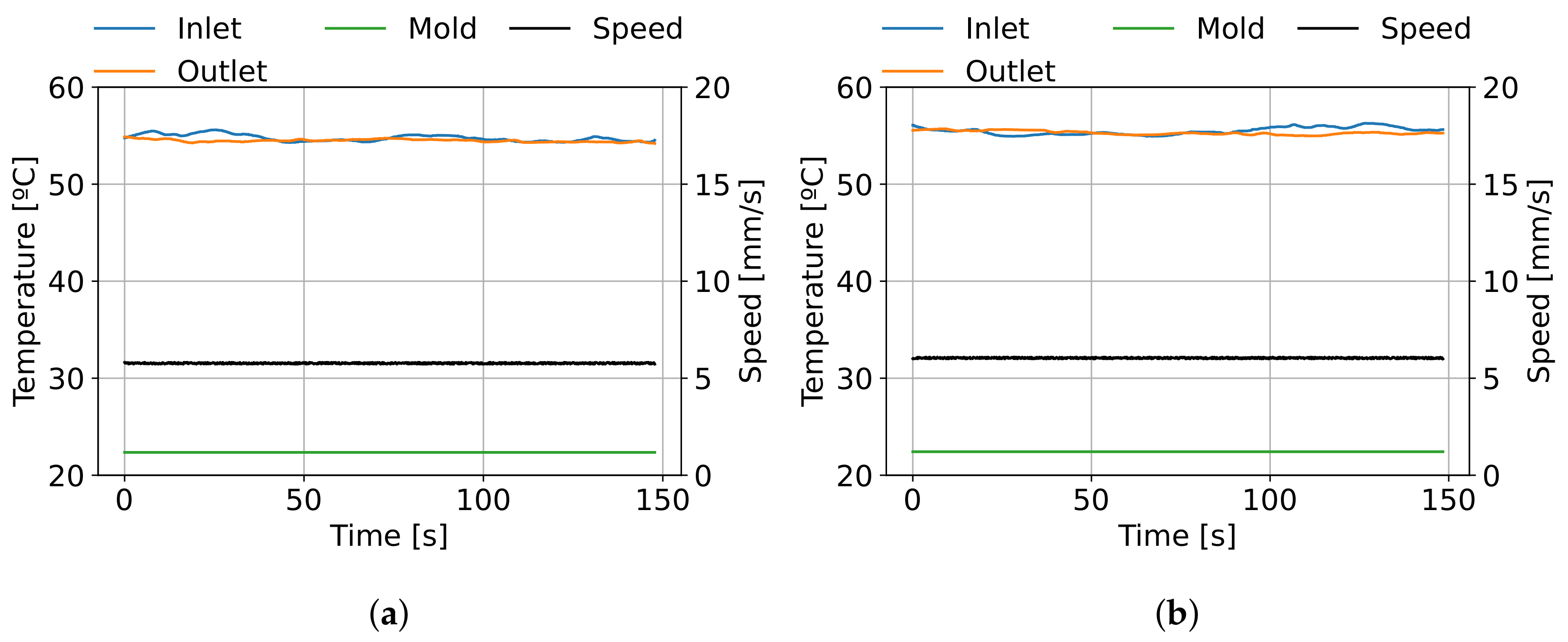
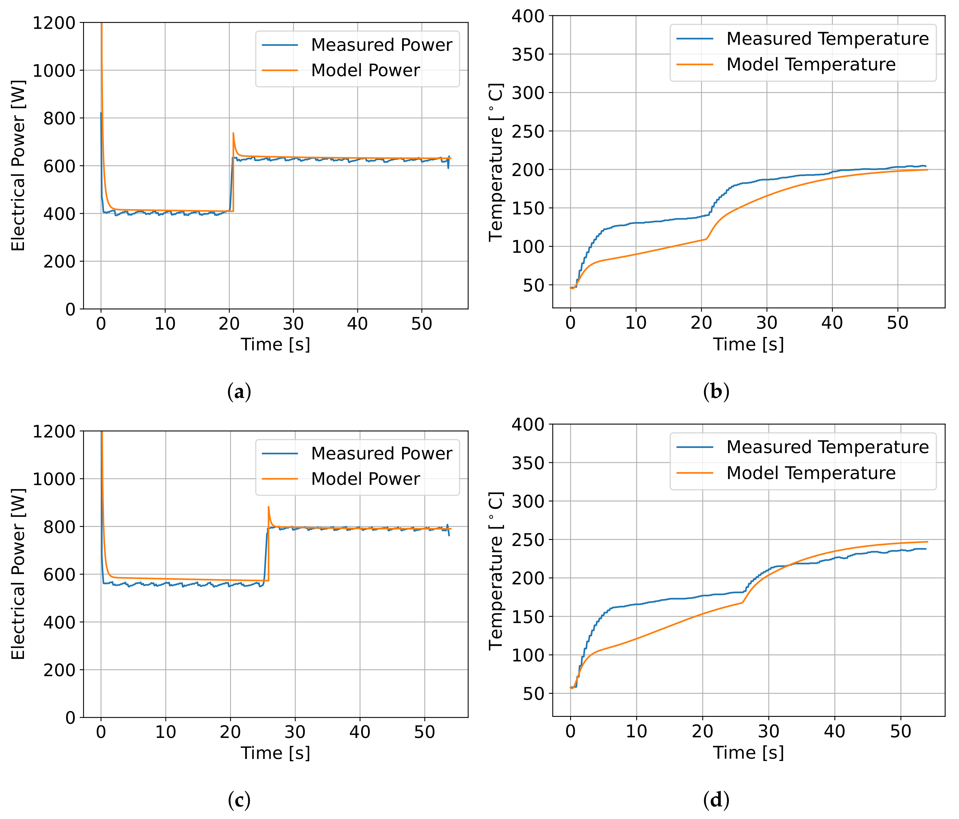
6.2. Model Validation
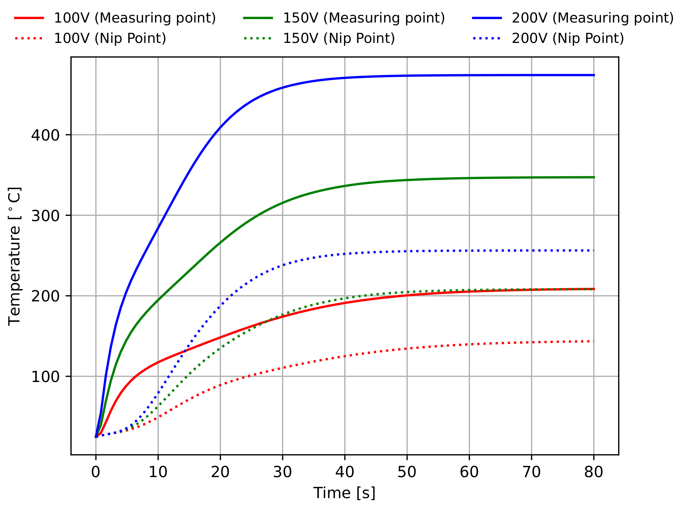
Sensitivity Analysis
7. Conclusions
Author Contributions
Funding
Institutional Review Board Statement
Informed Consent Statement
Data Availability Statement
Conflicts of Interest
References
- Engelhardt, R.; Ehard, S.; Wolf, T.; Oelhafen, J.; Kollmannsberger, A.; Drechsler, K. In Situ Joining of Unidirectional Tapes on Long Fiber Reinforced Thermoplastic Structures by Thermoplastic Automated Fiber Placement for Scientific Sounding Rocket Applications. Procedia CIRP 2019, 85, 189–194. [Google Scholar] [CrossRef]
- Comer, A.J.; Ray, D.; Obande, W.O.; Jones, D.; Lyons, J.; Rosca, I.; O’Higgins, R.M.; McCarthy, M.A. Mechanical characterisation of carbon fibre-PEEK manufactured by laser-assisted automated-tape-placement and autoclave. Compos. Part A Appl. Sci. Manuf. 2015, 69, 10–20. [Google Scholar] [CrossRef]
- Saenz-Castillo, D.; Martín, M.; Calvo, S.; Rodriguez-Lence, F.; Güemes, A. Effect of processing parameters and void content on mechanical properties and NDI of thermoplastic composites. Compos. Part A Appl. Sci. Manuf. 2019, 121, 308–320. [Google Scholar] [CrossRef]
- Barakat, E.; Tannous, M. Simulation of the tape laying process with steering of tapes: Bonding defects prevention using simulation. In Proceedings of the 2019 Fourth International Conference on Advances in Computational Tools for Engineering Applications (ACTEA), Beirut, Lebanon, 3–5 July 2019; pp. 1–7. [Google Scholar] [CrossRef]
- Crosky, A.; Grant, C.; Kelly, D.; Legrand, X.; Pearce, G. Fibre placement processes for composites manufacture. In Advances in Composites Manufacturing and Process Design; Elsevier: Amsterdam, The Netherlands, 2015; pp. 79–92. [Google Scholar] [CrossRef]
- Khan, M.A.; Mitschang, P.; Schledjewski, R. Identification of some optimal parameters to achieve higher laminate quality through tape placement process. Adv. Polym. Technol. 2010, 29, 98–111. [Google Scholar] [CrossRef]
- Liebsch, A.; Koshukow, W.; Gebauer, J.; Kupfer, R.; Gude, M. Overmoulding of consolidated fibre-reinforced thermoplastics - increasing the bonding strength by physical surface pre-treatments. Procedia CIRP 2019, 85, 212–217. [Google Scholar] [CrossRef]
- Tumkor, S.; Turkmen, N.; Chassapis, C.; Manoochehri, S. Modeling of heat transfer in thermoplastic composite tape lay-up manufacturing. Int. Commun. Heat Mass Transf. 2001, 28, 49–58. [Google Scholar] [CrossRef]
- Martín, M.; Rodríguez-Lence, F.; Güemes, A.; Fernández-López, A.; Pérez-Maqueda, L.; Perejón, A. On the determination of thermal degradation effects and detection techniques for thermoplastic composites obtained by automatic lamination. Compos. Part A Appl. Sci. Manuf. 2018, 111, 23–32. [Google Scholar] [CrossRef]
- Parlevliet, P.P.; Bersee, H.E.; Beukers, A. Residual stresses in thermoplastic composites - a study of the literature. Part III: Effects of thermal residual stresses. Compos. Part A Appl. Sci. Manuf. 2007, 38, 1581–1596. [Google Scholar] [CrossRef]
- Sonmez, F.O.; Hahn, H.T. Modeling of Heat Transfer and Crystallization in Thermoplastic Composite Tape Placement Process. J. Thermoplast. Compos. Mater. 1997, 10, 198–240. [Google Scholar] [CrossRef]
- Stokes-Griffin, C.M.; Compston, P.; Matuszyk, T.I.; Cardew-Hall, M.J. Thermal modelling of the laser-assisted thermoplastic tape placement process. J. Thermoplast. Compos. Mater. 2015, 28, 1445–1462. [Google Scholar] [CrossRef]
- Schaefer, P.M.; Gierszewski, D.; Kollmannsberger, A.; Zaremba, S.; Drechsler, K. Analysis and improved process response prediction of laser- assisted automated tape placement with PA-6/carbon tapes using Design of Experiments and numerical simulations. Compos. Part A Appl. Sci. Manuf. 2017, 96, 137–146. [Google Scholar] [CrossRef]
- Khan, M.A.; Mitschang, P.; Schledjewski, R. Tracing the Void Content Development and Identification of its Effecting Parameters during in Situ Consolidation of Thermoplastic Tape Material. Polym. Polym. Compos. 2010, 18, 1–15. [Google Scholar] [CrossRef]
- Stokes-Griffin, C.; Compston, P. A combined optical-thermal model for near-infrared laser heating of thermoplastic composites in an automated tape placement process. Compos. Part A Appl. Sci. Manuf. 2015, 75, 104–115. [Google Scholar] [CrossRef]
- Hosseini, S.M.A.; Baran, I.; van Drongelen, M.; Akkerman, R. On the temperature evolution during continuous laser-assisted tape winding of multiple C/PEEK layers: The effect of roller deformation. Int. J. Mater. Form. 2020, 14, 203–221. [Google Scholar] [CrossRef]
- Pitchumani, R.; Gillespie, J.W.; Lamontia, M.A. Design and Optimization of a Thermoplastic Tow-Placement Process with In-Situ Consolidation. J. Compos. Mater. 1997, 31, 244–275. [Google Scholar] [CrossRef]
- Pettersson, M.; Stenström, S. Modelling of an electric IR heater at transient and steady state conditions: Part I: Model and validation. Int. J. Heat Mass Transf. 2000, 43, 1209–1222. [Google Scholar] [CrossRef]
- Pettersson, M.; Stenström, S. Modelling of an electric IR heater at transient and steady state conditions: Part II: Modelling a paper dryer. Int. J. Heat Mass Transf. 2000, 43, 1223–1232. [Google Scholar] [CrossRef]
- Lichtinger, R.; Hörmann, P.; Stelzl, D.; Hinterhölzl, R. The effects of heat input on adjacent paths during Automated Fibre Placement. Compos. Part A Appl. Sci. Manuf. 2015, 68, 387–397. [Google Scholar] [CrossRef]
- Belnoue, J.P.; Mesogitis, T.; Nixon-Pearson, O.J.; Kratz, J.; Ivanov, D.S.; Partridge, I.K.; Potter, K.D.; Hallett, S.R. Understanding and predicting defect formation in automated fibre placement pre-preg laminates. Compos. Part A Appl. Sci. Manuf. 2017, 102, 196–206. [Google Scholar] [CrossRef]
- Colton, J.; Leach, D. Processing parameters for filament winding thick-section PEEK/carbon fiber composites. Polym. Compos. 1992, 13, 427–434. [Google Scholar] [CrossRef]
- Di Francesco, M.; Veldenz, L.; Dell’Anno, G.; Potter, K. Heater power control for multi-material, variable speed Automated Fibre Placement. Compos. Part A Appl. Sci. Manuf. 2017, 101, 408–421. [Google Scholar] [CrossRef]
- Silex. Silicone Rubber Sheeting High Temperature Solid, Datasheet. 2019. Available online: https://www.silex.co.uk/media/38087/solid-sheet-thtsilex-ntds.pdf (accessed on 2 February 2019).
- Narnhofer, M.; Schledjewski, R.; Mitschang, P.; Perko, L. Simulation of the Tape-Laying Process for Thermoplastic Matrix Composites. Adv. Polym. Technol. 2013, 32, E705–E713. [Google Scholar] [CrossRef]
- Chinesta, F.; Leygue, A.; Bognet, B.; Ghnatios, C.; Poulhaon, F.; Bordeu, F.; Barasinski, A.; Poitou, A.; Chatel, S.; Maison-Le-Poec, S. First steps towards an advanced simulation of composites manufacturing by automated tape placement. Int. J. Mater. Form. 2014, 7, 81–92. [Google Scholar] [CrossRef] [Green Version]
- Incropera, F.P.; DeWitt, D.P.; Bergman, T.L.; Lavine, A.S. Fundamentals of Heat and Mass Transfer, 6th ed.; John Wiley & Sons: Hoboken, NJ, USA, 2007. [Google Scholar] [CrossRef]
- Howell, J.; Menguc, M.; Siegel, R. Thermal Radiation Heat Transfer; CRC Press: Boca Raton, FL, USA, 2015. [Google Scholar]
- Modest, M. Radiative Heat Transfer, 3rd ed.; Academic Press: Cambridge, MA, USA, 2013; p. 904. [Google Scholar]
- Shapiro, A. FACET: A Radiation View Factor Computer Code for Axisymmetric, 2D Planar, and 3D Geometries with Shadowing; Lawrence Livermore National Lab.: Livermore, CA, USA, 1983. [Google Scholar]
- Pettersson, M. Heat Transfer and Energy Efficiency in Infrared Paper Dryers. Ph.D. Thesis, Lund University, Lund, Sweden, 1999. [Google Scholar]
- Forsythe, W.E.; Adams, E.Q. Radiating Characteristics of Tungsten and Tungsten Lamps A Correction. J. Opt. Soc. Am. 1945, 35, 306. [Google Scholar] [CrossRef]
- Izuegbu, N.S.; Adonis, M.L. Simulation and modelling of energy efficient design of a ceramic infrared heater. In Proceedings of the 2011 8th Conference on the Industrial and Commercial Use of Energy, ICUE 2011, Cape Town, South Africa, 16–17 August 2011; pp. 69–74. [Google Scholar]
- Lampinen, M.J.; Ojala, K.T.; Koski, E. Modeling and measurements of infrared dryers for coated paper. Dry. Technol. 1991, 9, 973–1017. [Google Scholar] [CrossRef]
- Venkateshan, S. Heat Transfer; Springer International Publishing: Cham, Switzerland, 2021; pp. 160–189. [Google Scholar] [CrossRef]
- Feingold, A.; Gupta, K.G. New analytical approach to the evaluation of configuration factors in radiation from spheres and infinitely long cylinders. J. Heat Transf. 1970, 92, 69–76. [Google Scholar] [CrossRef]
- Domalski, E.S. NIST Chemistry WebBook. 2011. Available online: https://webbook.nist.gov/ (accessed on 23 November 2021).
- Bansal, N.P. Handbook of Glass Properties; Elsevier: Amsterdam, The Netherlands, 1986; p. 680. [Google Scholar] [CrossRef]
- Sergeev, O.A.; Shashkov, A.G.; Umanskii, A.S. Thermophysical properties of quartz glass. J. Eng. Phys. 1982, 43, 1375–1383. [Google Scholar] [CrossRef]
- Chase, M.W.; Curnutt, J.L.; Downey, J.R.; McDonald, R.A.; Syverud, A.N.; Valenzuela, E.A. JANAF Thermochemical Tables, 1982 Supplement. J. Phys. Chem. Ref. Data 1982, 11, 695–940. [Google Scholar] [CrossRef] [Green Version]
- Gale, W.F.; Totemeier, T.C. Smithells Metals Reference Book, 8th ed.; Elsevier: Amsterdam, The Netherlands, 2003; Volume 1, p. 2080. [Google Scholar]
- Lide, D.R. (Ed.) CRC Handbook of Chemistry and Physics, 84th ed.; CRC Press LLC: Boca Raton, FL, USA, 2003; p. 2616. ISBN 0-8493-0484-9. [Google Scholar]
- Hust, J.G.; Lankford, A.B. Thermal Conductivity of Aluminium, Copper, Iron, and Tungsten for Temperatures from 1 K to the Melting Point; Number June; U.S. Department of Commerce: Washington, DC, USA, 1984; p. 266. [Google Scholar]
- Edwards, T.C.; Steer, M.B. Foundations for Microstrip Circuit Design, 4th ed.; John Wiley & Sons: Hoboken, NJ, USA, 2016. [Google Scholar]
- Wentink, T.; Planet, W.G. Infrared Emission Spectra of Quartz. J. Opt. Soc. Am. 1961, 51, 595. [Google Scholar] [CrossRef]
- Toray Group. Nylon 6-Based Thermoplastic Composite. 2019. Available online: https://www.toraytac.com/media/694245aa-3765-43b4-a2cd-8cf76e4aeec5/lmhIVg/TAC/Documents/Data_sheets/Thermoplastic/UD%20tapes,%20prepregs%20and%20laminates/Toray-Cetex-TC910_PA6_PDS.pdf (accessed on 23 November 2021).
- ASTM E 1269-9901. Standard Test Method for Determining Specific Heat Capacity by Differential Scanning Calorimetry; ASTM: West Conshohocken, PA, USA, 2001. [Google Scholar]
- Zhai, S.; Zhang, P.; Xian, Y.; Zeng, J.; Shi, B. Effective thermal conductivity of polymer composites: Theoretical models and simulation models. Int. J. Heat Mass Transf. 2018, 117, 358–374. [Google Scholar] [CrossRef]
- Villière, M.; Lecointe, D.; Sobotka, V.; Boyard, N.; Delaunay, D. Experimental determination and modeling of thermal conductivity tensor of carbon/epoxy composite. Compos. Part A Appl. Sci. Manuf. 2013, 46, 60–68. [Google Scholar] [CrossRef] [Green Version]
- Betta, G.; Rinaldi, M.; Barbanti, D.; Massini, R. A quick method for thermal diffusivity estimation: Application to several foods. J. Food Eng. 2009, 91, 34–41. [Google Scholar] [CrossRef]
- Yang, C.Y. Estimation of the temperature-dependent thermal conductivity in inverse heat conduction problems. Appl. Math. Model. 1999, 23, 469–478. [Google Scholar] [CrossRef]
- Optris. Compact IR Pyrometer for OEM Applications: Optris CS LT. 2021. Available online: https://www.optris.global/optris-cs-lt-csmed-lt (accessed on 23 November 2021).
- Hairer, E.; Wanner, G. Solving Ordinary Differential Equations II; Springer Series in Computational Mathematics; Springer: Berlin/Heidelberg, Germany, 1996; Volume 14. [Google Scholar] [CrossRef]


| Lamp Property | Measured Value |
|---|---|
| Lamp length | 189.02 mm ± 0.34 mm |
| Lamp diameter | 10.01 mm ± 0.19 mm |
| Lamp resistance (at 23 °C) | 9.6 ± 6.41 ·10 |
| Filament diameter | 0.410 mm ± 0.004 mm |
| Filament coil diameter | 2.890 mm ± 0.004 mm |
| Filament coil length | 290.04 mm ± 0.37 mm |
| Filament mass | 5.2019 g ± 0.0005 g |
| Lamp glass mass | 13.8780 g ± 0.0005 g |
| Parameter | Set 1 | Set 2 |
|---|---|---|
| Compaction roll temperature | ||
| Mold temperature | ||
| Process speed |
| Simulation | Parameters | Values |
|---|---|---|
| 1 | Compaction roll Temperature | 55 °C |
| Mold Temperature | 22 °C | |
| Speed | 5 mm/s | |
| Voltage | 100 V | |
| Voltage | 150 V | |
| Voltage | 200 V | |
| 2 | Compaction roll Temperature | 55 °C |
| Mold Temperature | 22 °C | |
| Voltage | 150 V | |
| Speed | 5 mm/s | |
| Speed | 10 mm/s | |
| Speed | 15 mm/s |
Publisher’s Note: MDPI stays neutral with regard to jurisdictional claims in published maps and institutional affiliations. |
© 2022 by the authors. Licensee MDPI, Basel, Switzerland. This article is an open access article distributed under the terms and conditions of the Creative Commons Attribution (CC BY) license (https://creativecommons.org/licenses/by/4.0/).
Share and Cite
de Sá Rodrigues, J.; Gonçalves, P.T.; Pina, L.; Gomes de Almeida, F. Modelling the Heating Process in the Transient and Steady State of an In Situ Tape-Laying Machine Head. J. Manuf. Mater. Process. 2022, 6, 8. https://doi.org/10.3390/jmmp6010008
de Sá Rodrigues J, Gonçalves PT, Pina L, Gomes de Almeida F. Modelling the Heating Process in the Transient and Steady State of an In Situ Tape-Laying Machine Head. Journal of Manufacturing and Materials Processing. 2022; 6(1):8. https://doi.org/10.3390/jmmp6010008
Chicago/Turabian Stylede Sá Rodrigues, Jhonny, Paulo Teixeira Gonçalves, Luis Pina, and Fernando Gomes de Almeida. 2022. "Modelling the Heating Process in the Transient and Steady State of an In Situ Tape-Laying Machine Head" Journal of Manufacturing and Materials Processing 6, no. 1: 8. https://doi.org/10.3390/jmmp6010008
APA Stylede Sá Rodrigues, J., Gonçalves, P. T., Pina, L., & Gomes de Almeida, F. (2022). Modelling the Heating Process in the Transient and Steady State of an In Situ Tape-Laying Machine Head. Journal of Manufacturing and Materials Processing, 6(1), 8. https://doi.org/10.3390/jmmp6010008