Development of a Novel Tuning Approach of the Notch Filter of the Servo Feed Drive System

Abstract

To alleviate the vibration effect of the feed drive system, a traditional approach is to apply notch filters to suppress vibrations in the velocity loop. The current approach is to adjust the notch filter parameters such as the center frequency, damping and depth based on observing the frequency response diagram of servo velocity closed loop. In addition, the notch filters are generally provided in the velocity loop control for the commercialized controllers such as FANUC, Siemens, etc. However, the resonance of the transmission system also appears in the position loop when the linear scale is used as the position feedback. The notch filter design without consideration of the resonance behavior of the position loop might cause degradation of performance. To overcome this problem, the paper proposes an innovative method which could automatically determine the optimal parameters of the notch filter under the consideration of resonance behavior of position loop. With the optimal parameters, it is found that both the gains of position and velocity loop controller could be increased such that the bandwidths of the position/velocity loops are higher. Based on the simulation results, the rising time is improved by 33% and the time for reaching the steady state is improved by 72% as comparing the cases of using the optimal approach and traditional approach.

1. Introduction

High-speed machine tools are widely used in manufacturing the parts for aviation, automotive, mold, and other industrial fields. The design objectives of machine tools are to obtain high efficiency, high precision and high surface quality. However, vibrations of machine structure may be excited when the machine is under high speed and acceleration condition, and the surface quality would also be affected. To avoid the vibration effects, many factors should be considered. One of the most critical factors is how to adjust the servo control parameters. The vibrations could deteriorate the manufacturing qualities and performances [1,2,3].

To suppress the structural vibration of the feed drive system, many scholars have proposed different approaches. For example, motion commands are filtered before entering the servo controller [4,5,6]. Some scholars have also proposed strategies that adopted active damping of structural vibrations inside the control loop [7,8,9]. In the modern time, there are many various ways to control vibration behavior, such as neural networks [10,11], fuzzy control [12,13], and sliding mode control [14,15]. These methods can achieve higher control bandwidth by applying notch filters in the control loop. However, the design of such controllers could be difficult because higher-order plant models need to be considered in order to include the vibration modes into the dynamic model. For commercialized controllers, the control loops are designed by three main loops: current, velocity and position loops. The commercial controllers generally apply the notch filters in velocity loop to alleviate the vibration signal near the resonance frequency [16] such that the bandwidth of the control loop could be increased. However, the traditional method of adjusting the notch filter only considers the resonance behavior of the velocity loop. The resonance behaviors of the components located outside the velocity loop have not been considered. The research of how to design the notch filter by considering both the velocity and position loop dynamics is still an open issue. In this paper, a novel approach which could determine the optimal parameters of the notch filter is proposed. In the approach, the vibration effects in velocity and position loops are considered, and the parameters of notch filters could automatically be adjusted. The paper is arranged as follows. In Section 2, the dynamics of the feed system and the traditional approach are introduced. Then, the novel optimal approach is proposed in Section 3. The Bode plots velocity and position loop of using traditional and optimal approaches are compared in Section 4. The servo performances using the traditional and optimal approaches for the step input and the trajectory are compared. Finally, Section 5 gives the conclusion.

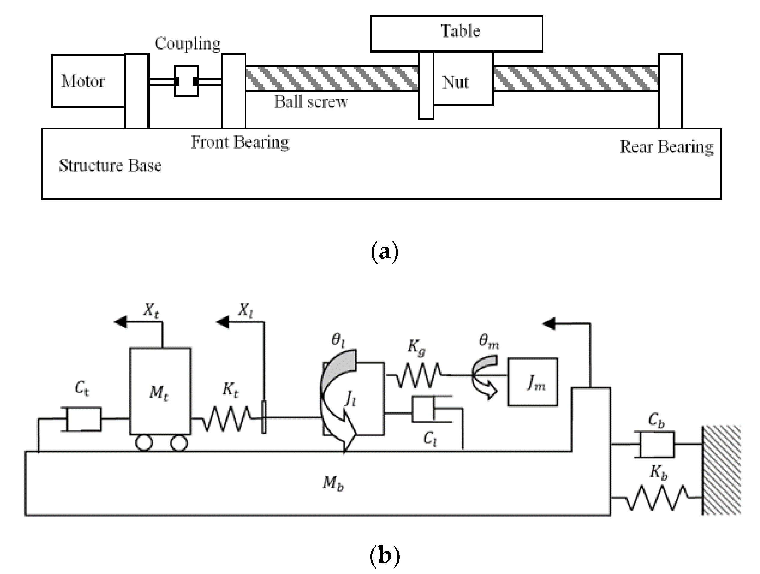
2. The Dynamic Model of the Feed Drive System

In this section, the dynamic model of the feed drive system is first derived. Then, the dynamic model is simplified to explain the parameter tuning process.

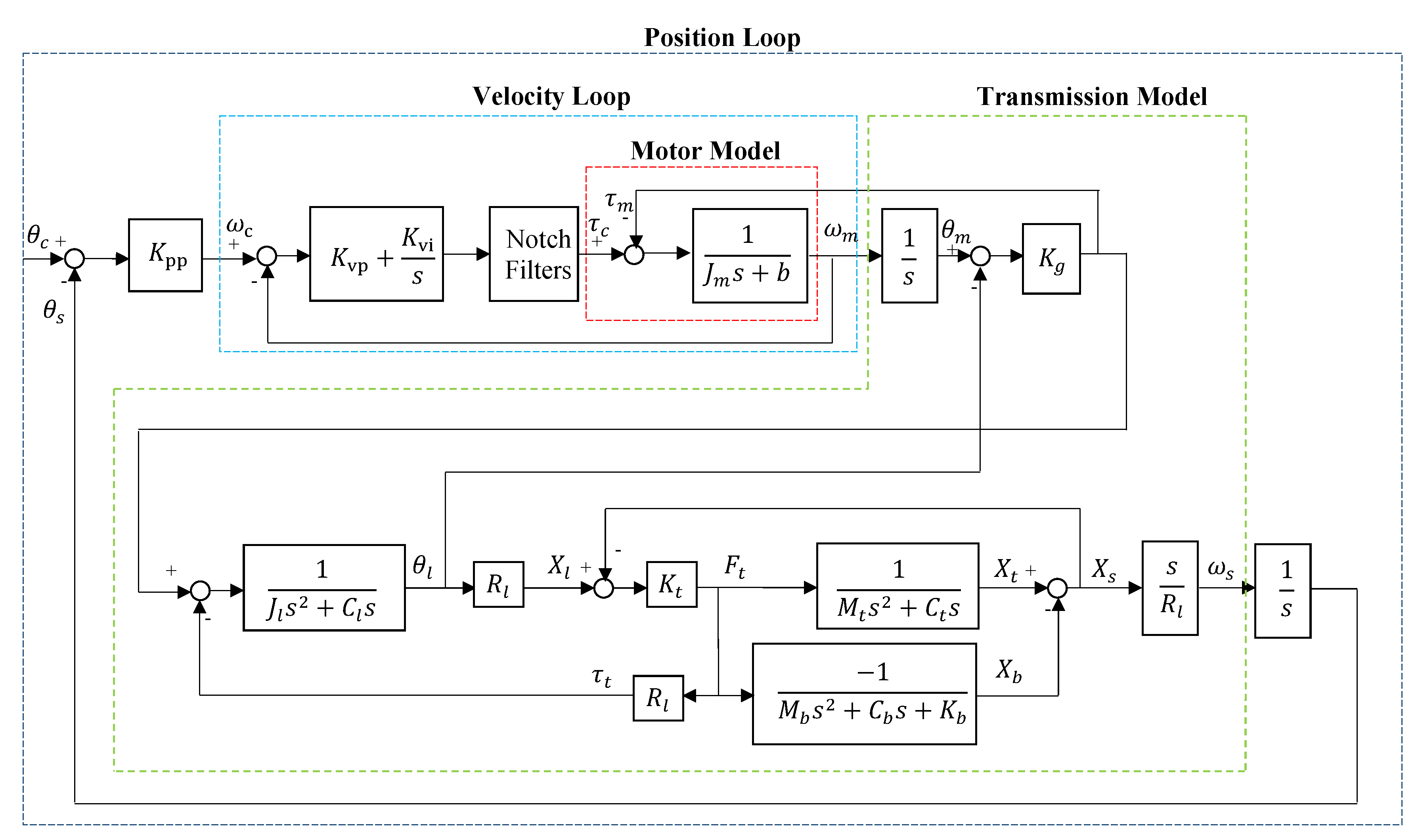
2.1. The Derivation of the Feed Drive System

To describe the dynamic behavior of feed drive system, this paper utilizes the model proposed by the paper [4]. The model includes the dynamics effects of couplings, ball-screws, structure base, and servo loop controls. The schematic diagram of a feed drive system is shown in Figure 1a. The rotary motion of the motor drives the platform through the coupling and the ball-screw. The rotation of the motor can be measured by the encoder mounted on the motor. The linear motion of the platform can be measured by the optical linear scale on the platform. The feed drive system can be simplified as a mass-damper-spring (MCK) system as shown in Figure 1b.

In Figure 1, the parameters could be defined as the following. $X_t$ is the displacement of the table, $X_l$ is the displacement of the ball-screw, and $X_b$ is the displacement of the base. ${\theta }_l$ and ${\theta }_m$ are the ball-screw and motor rotation angle. $J_l$ and $J_m$ are the inertia of the ball-screw and motor. $M_t$ and $M_b$ are the mass of table and base. $C_t$, $C_l$ and $C_b$ are the damping of guideway, ball-screw and base, respectively. $K_b$, $K_g$ and $K_t$ are the stiffness of base, coupling stiffness and longitudinal stiffness of ball-screw, respectively. The rotary motion of the ball-screw, ${\theta }_l$, is transmitted to the linear displacement, $X_l$, through the converting ratio, $R_l$. $R_l$ is given as $P/2\pi$, where $P$ is the pitch of the ball-screw.

After the integration of the feed drive system and servo loop control system, the complete system can be expressed as the block diagram shown in Figure 2 and is named as the servo feed drive system. The figure can be divided into four subsystems such as motor model, the transmission model, the velocity loop and the position loop. The four parts can be introduced as follows.

In the motor model, ${\tau }_c$ is the motor torque, $b$ is the friction torque of the motor, ${\omega }_m$ is the motor angular velocity, and ${\tau }_m$ is the torque which is generated by the resonance behavior of the transmission model.

The velocity loop consists of the velocity controller, the notch filters, and the motor model. The velocity controller includes proportional gain $K_{vp}$ and integral gains $K_{vi}$; the controller is designed to control the motor model under different effects. The notch filters are used for suppressing the resonance behavior and it can be represented as Equation (1). In the Equation, ${\omega }_n$, ${\zeta }_n$ and ${\kappa }_n$ are the center frequency, damping and depth of the notch filter, respectively. The Bode plot of the notch filter is shown in Figure 3.

$$N\left(s\right)=\frac{s^2+2{\zeta }_n {\omega }_n s+{{\omega }_n}^2}{s^2+2{\zeta }_n {\kappa }_n {\omega }_n s+{{\omega }_n}^2}$$

(1)

In the transmission model, the input of the model is the motor angular velocity ${\omega }_m$, and the output is the velocity ${\omega }_s$ of the moving platform, which is related to the linear displacement $X_s$ by ${\omega }_s=s{X}_s/R_l$. The transmission model is described by the transfer function between ${\omega }_s$ and ${\omega }_m$.

The outer loop is the position loop, which contains the velocity loop, the transmission model and the position controller. The position controller is a proportional gain and is represented as $K_{pp}$. The parameters of the servo feed drive system are identified from the experiment [4] as shown in

Table 1. Parameters of the servo feed drive system.

Parameters	Value (Unit)	Parameters	Value (Unit)
$C_b$	800 (Ns/m)	$K_g$	8520 (Nm/rad)
$C_l$	1.95 (Ns/m)	$K_t$	1.95 ×${10}^8$ (N/m)
$C_t$	500 (Ns/m)	$M_t$	138 (kg)
$J_l$	0.00823 (${\mathrm{kgm}}^2)$	$M_b$	570 (kg)
$J_m$	0.04 (${\mathrm{kgm}}^2)$	$R_l$	0.0032 (m/rad)
$K_b$	1.83 ×${10}^6$ (N/m)	$b$	0.003342 (Nms/rad)
$K_f$	1.38 ($\mathrm{Nm}/A$)

.

In order to explain the influence of the feed drive system on the design of the servo loop, the model is divided into different modules for simplification, which would be explained in the following paragraphs.

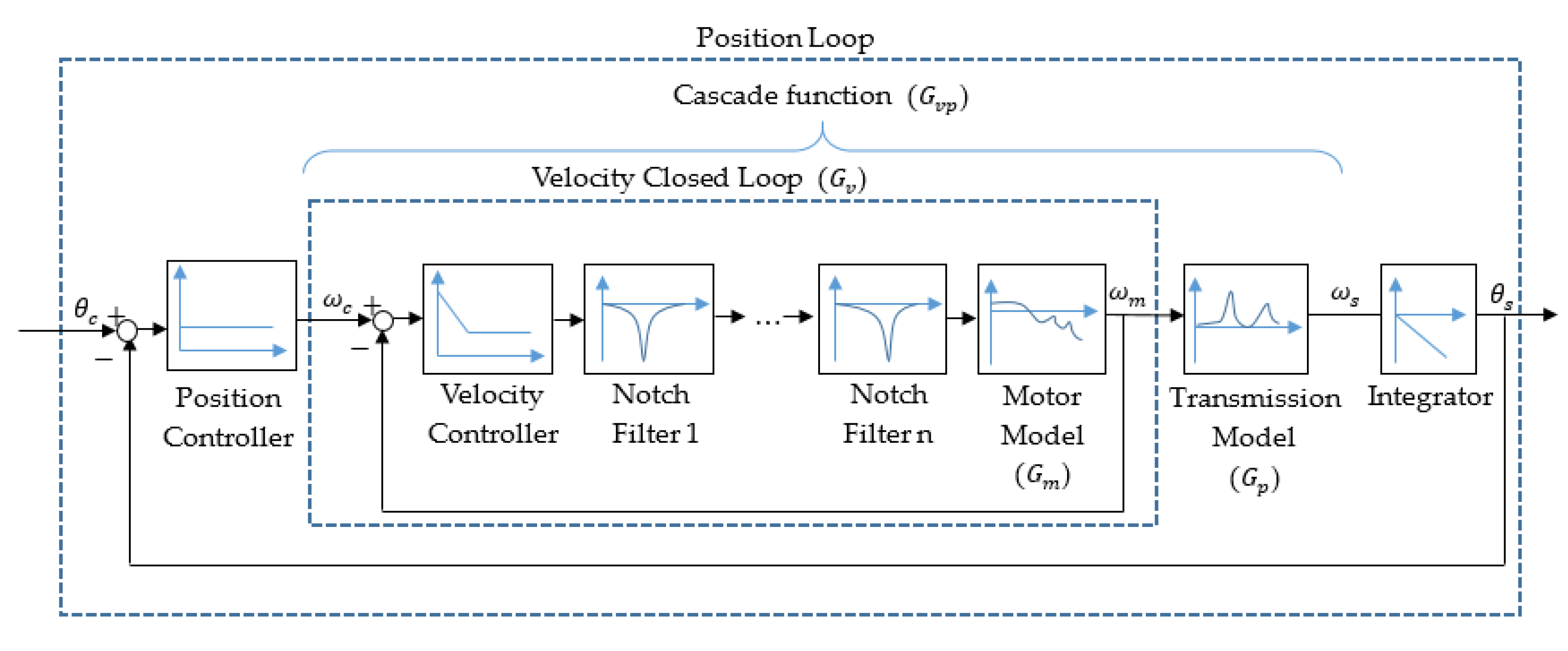
2.2. Transformed Representation of the Servo Feed Drive System

In this section, in order to discuss the impact caused by motor and transmission models, the feed drive system shown in Figure 2 is transformed into different representations as shown in Figure 4 where the motor and transmission models are obtained by Mason rules and the respective transfer functions G_m and $G_p$ are given as follows.

$$\begin{array}{c}{G}_m=\frac{G_{1}s\left(K_g{G}_2+K_t{G}_3-K_t{G}_4+K_g{K}_t{G}_2{G}_3-K_g{K}_t{G}_2{G}_4-{R_1}^2{K}_t{G}_2+1\right)}{s\left(K_g{G}_2+K_t{G}_3-K_t{G}_4+K_g{K}_t{G}_2{G}_3-K_g{K}_t{G}_2{G}_4-R_l{K}_t{G}_2{G}_4+1\right)+K_g{G}_1+K_g{K}_t{G}_1{G}_3-K_g{K}_t{G}_1{G}_4}\\ G_p=\frac{K_g{R}_l{K}_{t}s{G}_2\left(G_3-G_4\right)}{R_{l}s\left(K_g{G}_2+K_t{G}_3-K_t{G}_4+K_g{K}_t{G}_2{G}_3-K_g{K}_t{G}_2{G}_4-R_l{K}_t{G}_2{G}_4+1\right)}\\ G_1=\frac{1}{J_{m}s+b},G_2=\frac{1}{J_l{s}^2+C_{l}s},G_3=\frac{1}{M_t{s}^2+C_{t}s}, G_4=\frac{-1}{M_b{s}^2+C_{b}s+K_b}\end{array}$$

(2)

The velocity loop transfer function between ${\omega }_c$ and ${\omega }_m$ is defined as $G_v$. $G_{vp}$ is given as $G_v{G}_p$, which is the cascaded function of velocity loop $G_v$ and the transmission model $G_p$. The transformed representation could provide a more systematic approach to evaluate the dynamics within the velocity loop $G_v$ and the dynamics outside of the velocity loop $G_p$. Figure 4 motivates the objective of this paper for designing the notch filter with or without consideration of $G_p$.

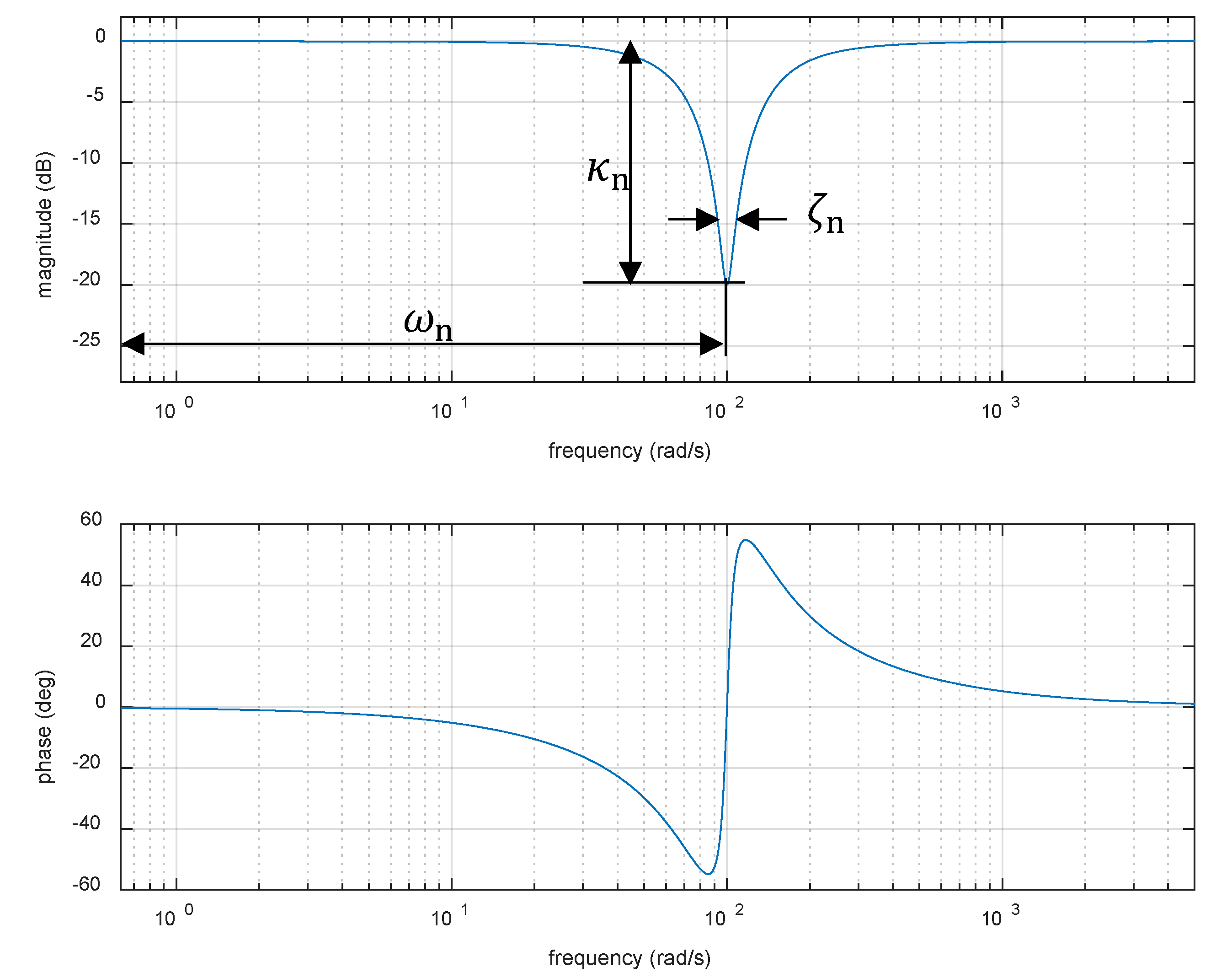
2.3. Traditional Tuning Method of Notch Filter

The process of the traditional tuning method of the controller is to tune the parameter of the velocity loop to a higher bandwidth. Then, the position loop parameter is then tuned based on either Bode plot or step response. However, when tuning the controller in the velocity loop, the resonance behavior outside the velocity loop, such as the resonance behavior of transmission model, would not be considered. To avoid vibration, the notch filter is applied in the velocity loop. The traditional approach to tune the parameters of notch filter only consider the dynamics of velocity loop based on the frequency response of the velocity closed loop. The resonance could be identified and the three parameters in Equation (1) could be found consequently. After tuning, the dynamics response of the velocity loop is generally smooth. However, the resonance behavior occured in a position loop because both velocity loop and position loop contain the resonance behavior as shown in Figure 4. Generally, the resonance behavior in the position loop cannot be suppressed because the position controller is a position gain $K_{pp}$ and has no notch filter. As the result, the $K_{pp}$ cannot be adjusted too high to avoid exciting the resonance.

Although using the traditional method could allow the controller parameters to be easily designed, the bandwidth of the position loop is quite limited. One systematical approach is to consider both the position and velocity loops simultaneously when designing the parameters of notch filter.

3. The Notch Filter Tuning Approach Using the Optimization

In this section, an optimization design methodology for the notch filter is proposed such that the resonance behaviors of the motor and transmission models in position loop can be suppressed as well. The range of the center frequency of the notch filter is firstly determined by Nyquist plot of the motor model as follows.

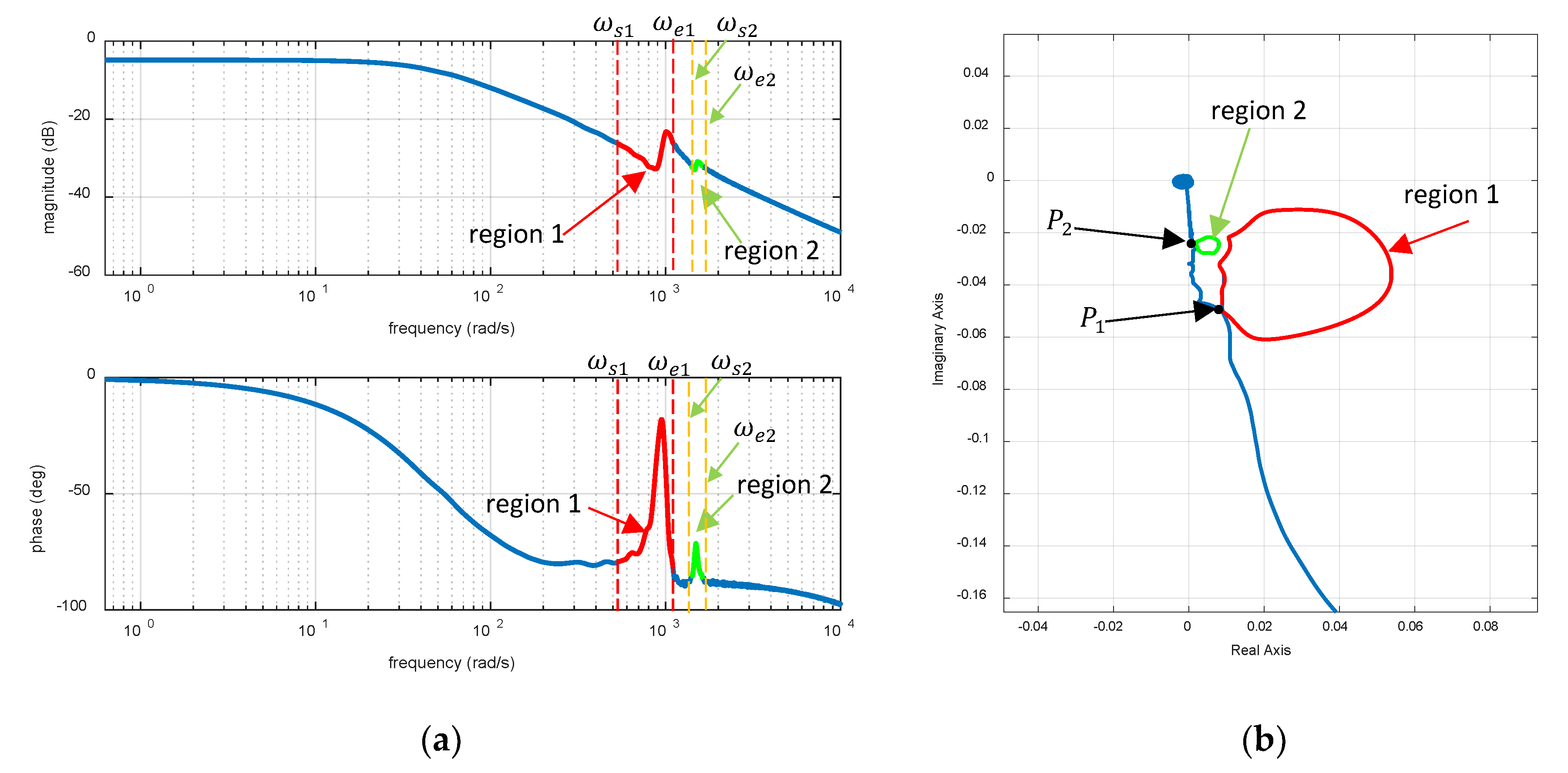
3.1. The Determination of the Range of the Center Frequency by Nyquist Plot

Using the parameters listed in Table 1, the Bode plot of $G_m$ is shown in Figure 5a where the two resonances occur at about 1000 and 1500 (rad/s). The Nyquist diagram shown in Figure 5b indicates that the frequency curves around each resonance will form a circle due to the phase changes within the region 1 and 2. The ${\omega }_{s1}$ and ${\omega }_{e1}$ in Figure 5a correspond to the same point of $P_1$ in Figure 5b. Taking region 1 as an example, by searching the intersection point $P_1$, one can locate the first resonance range. The searching of ${\omega }_s$ and ${\omega }_e$ is to let the following function equal to 0.

$$L=\sqrt{{\left(Re\left(G_m\left(j{\omega }_s\right)-G_m\left(j{\omega }_e\right)\right)\right)}^2+{\left(Im\left(P\left(j{\omega }_s\right)-P\left(j{\omega }_e\right)\right)\right)}^2}$$

(3)

In this case, the ${\omega }_{s1}$ is equal to 534 (rad/s) and ${\omega }_{e1}$ is equal to 1100 (rad/s). The resonance in region 1 occurs within (534,1100) (rad/s). Using the same approach, one can determine the ${\omega }_{s2}$ and ${\omega }_{e2}$ equal to 1400 and 1628 (rad/s) for region 2.

3.2. Optimal Approach for Tuning Notch Filter

After locating the range of the center frequency, the optimization approach is to search the parameter of the notch filter such that the transfer function $G_{vp}$ become a smooth curve since the $G_{vp}$ contains both the dynamics of the velocity loop and position loop. The tuning process is given as three major steps.

• Determine the start frequency ${\omega }_s$ and end frequency ${\omega }_e$ of each closed path using the searching method in Section 3.1.
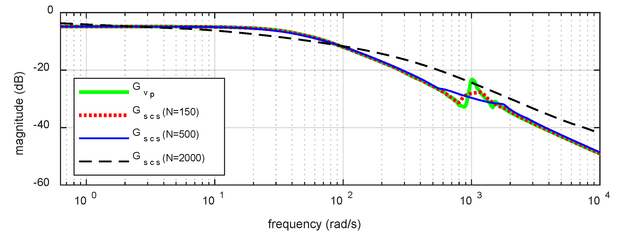
• Smooth $G_{vp}$ by applying the moving average filter $H$ given as the following.

  $$G_{scs}\left(s\right)=G_{vp}\left(s\right)H\left(s\right),H\left(s\right)=\frac{1}{N}\frac{1-e^{-sTN}}{1-e^{-sT}}$$

  (4)
  Here $G_{scs}$ is the smoothed transfer function of $G_{vp}$. The magnitude plot of $G_{vp}$ and three cases of $G_{scs}$ with different $N$ are shown in Figure 6. In the figure, it can be observed that $G_{scs}$ with smaller $N$ has a worse result; however, $G_{scs}$ with larger $N$ are changed completely and also have an unsuitable result. Hence, here the $N$ is selected as 500 to remain the main profile of $G_{vp}$ and smooth the peak parts of $G_{vp}$.
• The notch filter such that the resulting $G_{vp}$ can approach the $G_{scs}$ by minimizing the following objective function. The lower and upper bounds are obtained from step 1.

  $$J={{\displaystyle \int }}_{{\omega }_s}^{{\omega }_e}\left|G_{scs}\left(j\omega \right)-G_{vs}\left(j\omega \right)\right|d\omega$$

  (5)

By applying the particle swarming optimization [17], the optimal depth, damping and center frequency of the notch filter can be obtained. According to the content of Section 3.1, the resonance behavior of the plant occurs in two regions and they are within (534,1100) and (1400,1628) (rad/s), respectively. Because the resonance behavior is more serious and its frequency range is wider, we chose two notch filters (notch filter 1 and notch filter 2) in the first region and adopt one notch filter (notch filter 3) in the second region, and

Table 2. The sets of the notch filters for PSO optimization.

Transfer Function	Parameter	Initial Value	Minimum Value	Maximum Value	Unit
Notch Filter 1	${\omega }_1$	534	534	1100	rad/s
	${\zeta }_1$	0.1	0.1	10	-
	${\kappa }_1$	0.1	0.1	50	-
Notch Filter 2	${\omega }_2$	534	534	1100	rad/s
	${\zeta }_2$	0.1	0.1	10	-
	${\kappa }_2$	0.1	0.1	50	-
Notch Filter 3	${\omega }_3$	1400	1400	1628	rad/s
	${\zeta }_3$	0.1	0.1	10	-
	${\kappa }_3$	0.1	0.1	50	-

expresses the sets of the three notch filters for determining the optimal parameter through PSO. In Table 2, the center frequencies of the notch filters are limited within (534,1100) or (1400,1628) (rad/s), the other parameters such as damping and depth of the notch filters are within a wider range, and the initial values are the same as the minimum values.

Because the notch design could approach our desired smooth $G_{scs}$, the advantage is that both $G_p$ and $G_v$ are included in the design process. In the next section, the comparisons of using traditional and optimal approaches in time and frequency domains are discussed.

4. Results and Discussion

In this section, a comparison is given for the frequency response functions and the dynamic behavior of the feed drive system for the traditional and optimal approaches.

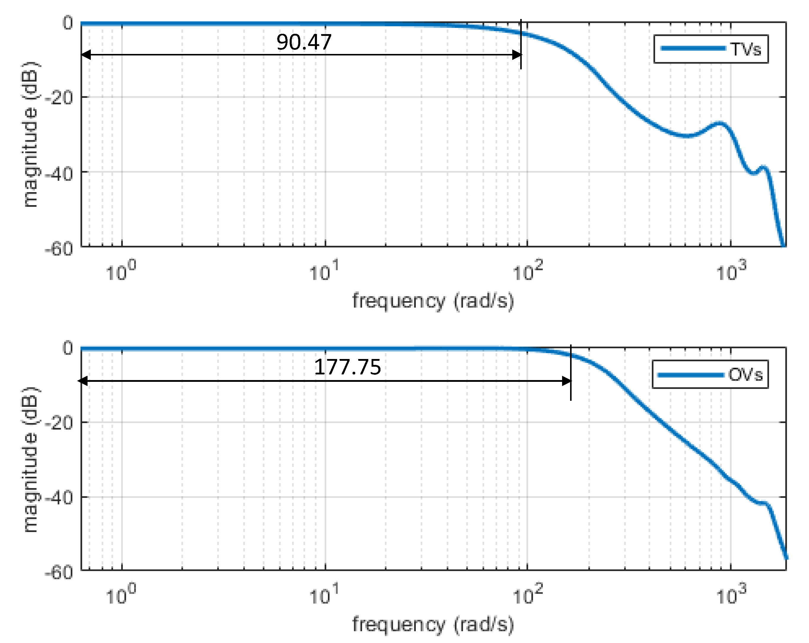
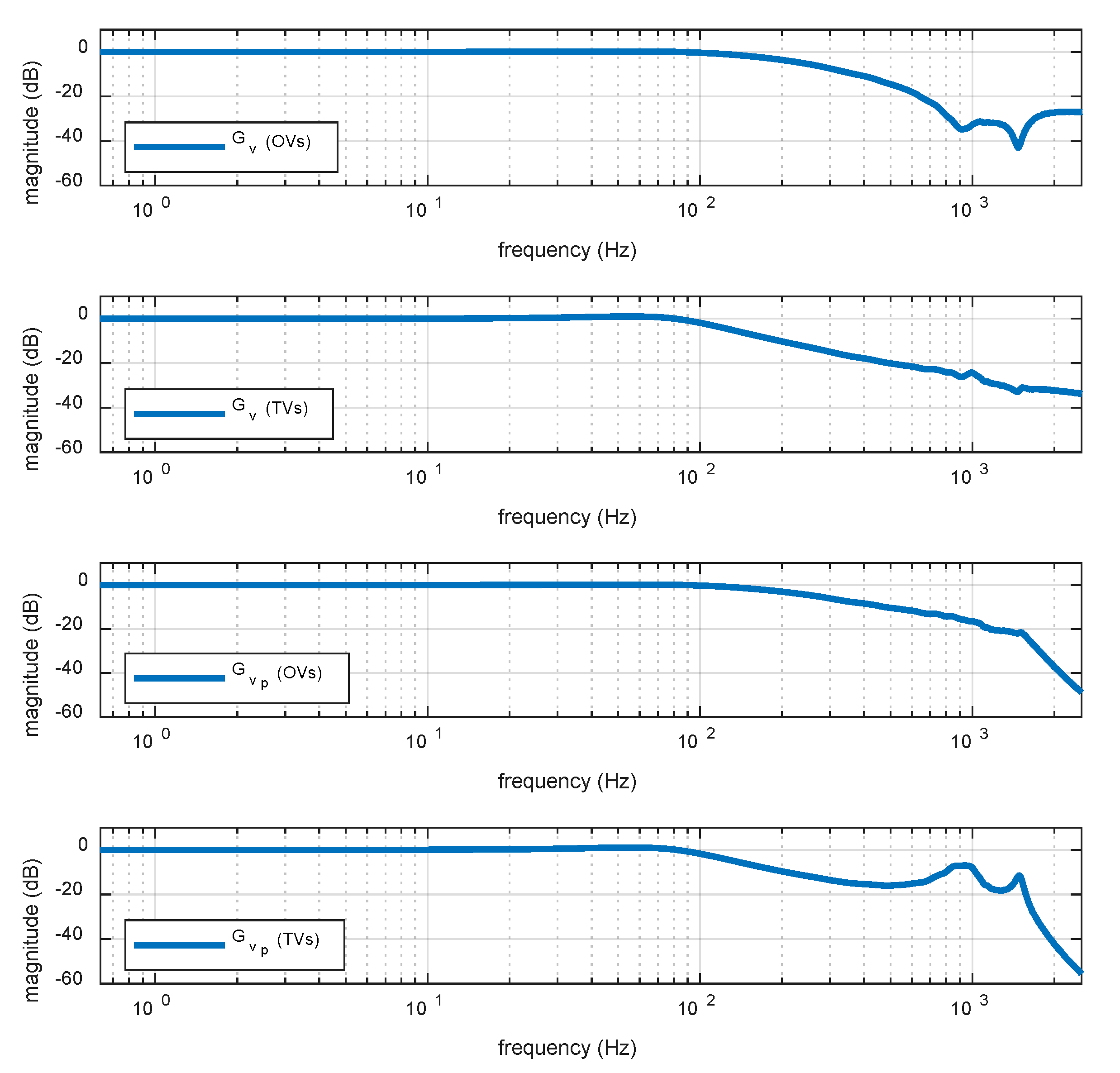
4.1. The Comparisons of Frequency Response Functions Using Traditional and Optimal Approaches

The parameters for traditional and optimal approaches are shown in

Table 3. The parameter values of optimal and traditional approaches.

Parameter	Traditional Value	Optimal Value	Unit
$K_{pp}$	92.47	298.41	1/s
$K_{vi}$	223.46	280.65	Nm $s^2$/rad
$K_{vp}$	1.78	4.46	Nms/rad
${\omega }_1$	1012.13	1099.92	rad/s
${\zeta }_1$	0.10	0.17	-
${\kappa }_1$	13.28	4.60	-
${\omega }_2$	884.33	988.31	rad/s
${\zeta }_2$	1.11	0.05	-
${\kappa }_2$	0.10	2.97	-
${\omega }_3$	1570.05	1485.52	rad/s
${\zeta }_3$	0.1	0.03	-
${\kappa }_3$	1.2	5.48	-

. Figure 7 shows the Bode plots of the velocity closed loop $G_v$ and the function $G_{vs}$ with traditional values (TVs) and optimal values (OVs). It is shown that the $G_v$ with TVs could suppress the resonance of the motor model $G_m$ completely. However, the resonances of $G_{vp}$ might hinder the increase of position gain. By using the OVs, the notch filter is designed to be deeper in order to compensate the resonance effect of $G_p$. Therefore, the $G_{vp}$ is smoother than $G_{vp}$ using the traditional approach.

To further investigate the effects on the position loop, the Bode plots of position loop for both cases are shown in Figure 8. Here, the $K_{pp}$ for both cases shown in Table 3 are chosen to be the maximum values such that the overshoot is less than 5%. It is shown that the bandwidth of position closed-loop with TVs is 90.47 (rad/s), and the bandwidth of position closed-loop with OVs is 177.75 (rad/s). The bandwidth is increased by 96% through using OVs.

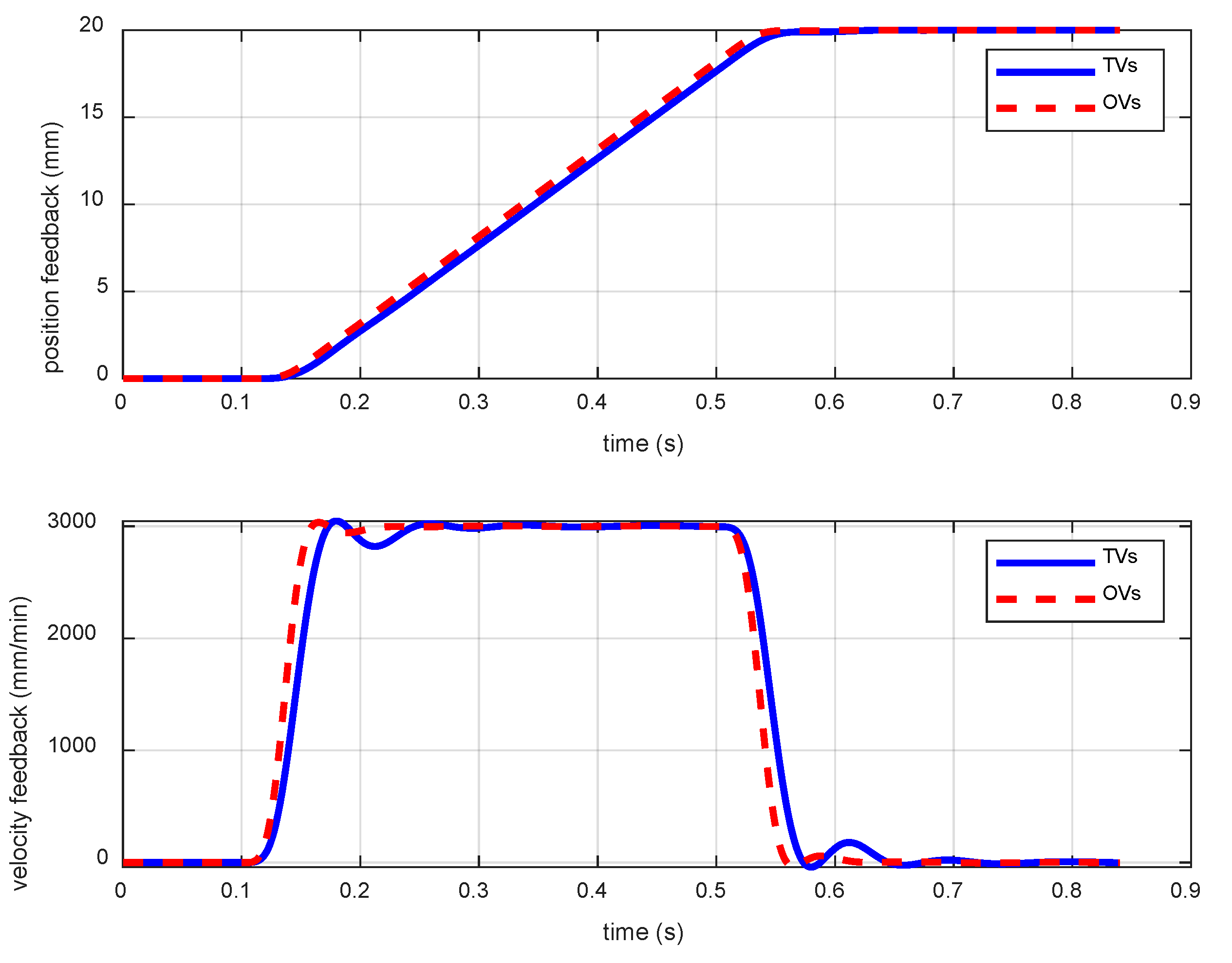
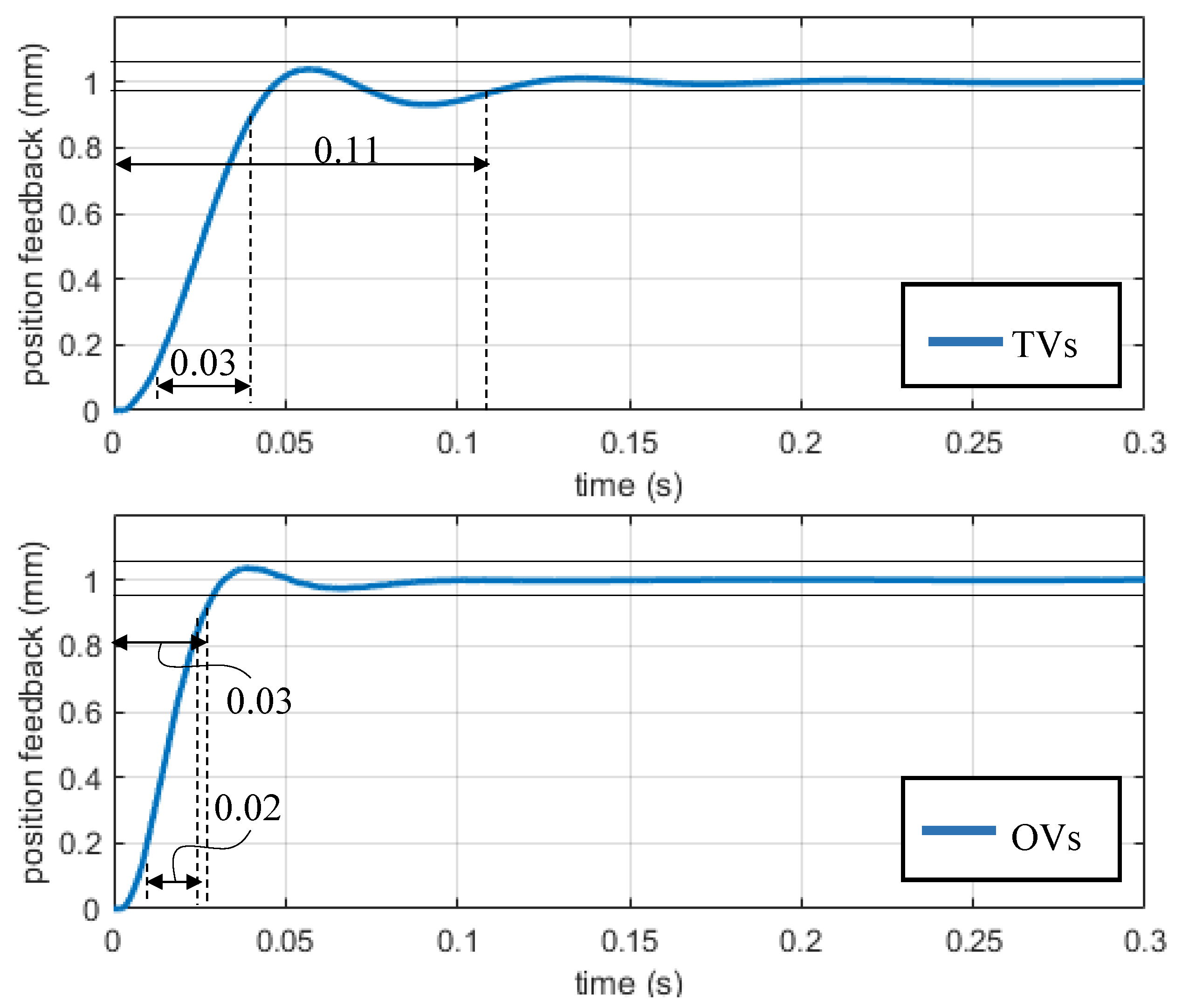
4.2. The Comparision of Simulation Results with Traditional and Optimal Parameters

The time domain simulations for one step response and one trajectory are conducted to compare the performances of the cases using the TVs and OVs.

As shown in Figure 9, the step responses for the input ${\theta }_c$ are shown in Figure 4. The output is the linear scale $X_s$. It could be found that the rising time of the system with TVs is 0.03 s and that with OVs is 0.02 s. The time to reach the steady state with TVs is 0.11 s and with OVs is 0.03 s where the case using OVs could improve by 72%. Because the bandwidth of the closed loop using TVs is higher, a quick response time can be expected. To validate that the algorithm can be applied in real machining, the results of the trajectory are performed.

Position commands of the trajectory under given velocity and accelerations are shown in the upper subfigure of Figure 10. The trajectory is given with a displacement, velocity and acceleration equals to 20 (mm), 3000 (mm/min), and 5000 $(\mathrm{mm}/s^2)$, respectively. The simulation results of using traditional and optimal parameters are shown in the lower subfigure of Figure 10. It can be observed that the system with OVs has a higher response and less resonance behavior as compared to the case with TVs. Again, it validates the advantages of using the optimal design approach for a notch filter.

5. Conclusions

Generally, the parameter determination of the notch filter is based on trial and error. In this paper, a systematical approach is proposed to obtain the optimal parameters of the notch filter. The first contribution of the paper is to derive the transformed block diagram, which could separate the dynamics within the velocity loop and outside the velocity loop. In order to locate the resonance range of center frequency, the Nyquist diagram is applied to find the intersection point which could be used in the optimization process. The second contribution of the paper is to use the moving average filter to specify the desired loop transfer function of the position loop. By applying the PSO method, one can determine the center frequency, damping and depth of notch filter at one time. The frequency response function of position closed loop shows that the bandwidth could increase compared to the tradition parameter approach and optimal approach. Furthermore, the rising time and steady state time of the step response are improved by 33% and 72%, respectively. In order to validate that the optimal approach can be applied to real machining, the trajectory with equal velocity and acceleration is tested. It is shown that the system with has higher response and less resonance behavior as compared to the case using the traditional approach.

References

1. Pritschow, G. On the Influence of the Velocity Gain Factor on the Path Deviation. Ann. CIRP 1996, 45, 367–371. [Google Scholar] [CrossRef]
2. Chen, Y.C.; Tlusty, J. Effect of Low-Friction Guideways and Lead-Screw Flexibility on Dynamics of High-Speed Machines. Ann. CIRP 1995, 44, 353–356. [Google Scholar] [CrossRef]
3. Pritschow, G. A Comparison of Linear and Conventional Electromechanical Drives. Ann. CIRP 1998, 47, 541–548. [Google Scholar] [CrossRef]
4. Tsai, M.S.; Huang, Y.C.; Lin, M.T.; Wu, S.K. Integration of Input Shaping Technique with Interpolation for Vibration Suppression of Servo-feed Drive System. J. Chin. Inst. Eng. 2017, 40, 284–295. [Google Scholar] [CrossRef]
5. Jones, S.D.; Ulsoy, A.G. An Approach to Control Input Shaping with Application to Coordinate Measuring Machines. ASME J. Dyn. Syst. Meas. Control 1999, 121, 242–247. [Google Scholar] [CrossRef]
6. Cole, M.O.T.; Shinonawanik, P.; Wongratanaphisan, T. Time-domain Prefilter Design for Enhanced Tracking and Vibration Suppression in Machine Motion Control. Mech. Syst. Signal Process. 2018, 104, 106–119. [Google Scholar] [CrossRef]
7. Symens, W.; Van Brussel, H.; Swevers, J. Gain-Scheduling Control of Machine Tools with Varying Structural Flexibility. Ann. CIRP 2004, 52, 321–324. [Google Scholar] [CrossRef]
8. Zheng, H.; Qin, H.; Ren, M.; Zhang, Z. Active Vibration Control for the Time-Varying Systems with a New Adaptive Algorithm. J. Vib. Control 2020, 26, 200–213. [Google Scholar] [CrossRef]
9. Ast, A.; Braun, S.; Eberhard, P.; Heisel, U. An Adaptronic Approach to Active Vibration Control of Machine Tools with Parallel Kinematics. Prod. Eng. 2009, 3, 207–215. [Google Scholar] [CrossRef]
10. Abdeljaber, O.; Avci, O.; Inman, D.J. Active Vibration Control of Flexible Cantilever Plates using Piezoelectric Materials and Artificial Neural Networks. J. Sound Vib. 2016, 363, 33–53. [Google Scholar] [CrossRef]
11. Yousefi, H.; Hirvonen, M.; Handroos, H. Application of Neural Network in Suppressing Mechanical Vibration of a Permanent Magnet Linear Motor. Control Eng. Pract. 2008, 16, 787–797. [Google Scholar] [CrossRef]
12. Edalath, S.; Kukreti, A.R.; Cohen, K. Enhancement of a Tuned Mass Damper for Building Structures using Fuzzy Logic. J. Vib. Control 2012, 19, 1763–1772. [Google Scholar] [CrossRef]
13. Thenozhi, S.; Yu, W. Active Vibration Control of Building Structures using Fuzzy Proportional-derivative/Proportional-integral-derivative Control. J. Vib. Control 2015, 21, 2340–2359. [Google Scholar] [CrossRef]
14. Yiǧit, I. Model Free Sliding Mode Stabilizing Control of a Real Rotary Inverted Pendulum. J. Vib. Control 2017, 23, 1645–1662. [Google Scholar] [CrossRef]
15. Wang, J.; Jin, F.; Zhou, L. Implementation of Model-free Motion Control for Active Suspension Systems. Mech. Syst. Signal Process. 2019, 119, 589–602. [Google Scholar] [CrossRef]
16. Smith, A.D. Wide Bandwidth Control of High-Speed Milling Machine Feed Drives. Ph.D. Thesis, University of Florida, Gainesville, FL, USA, 1999. [Google Scholar]
17. Kennedy, J.; Eberhart, R. Particle Swarm Optimization. Int. Conf. Neural Netw. IEEE 1995, 4, 1942–1948. [Google Scholar]
Figure 1. The feed drive system. (a) The schematic of the feed drive system. (b) The 2 DOF diagram of the feed drive system.
Jmmp 04 00021 g001
Figure 2. The block diagram of the servo feed drive system.
Jmmp 04 00021 g002
Figure 3. The Bode plot of the notch filter as ω n = 100 (rad/s), ζ n = 0.05 , and κ n = 20 (dB).
Jmmp 04 00021 g003
Figure 4. The transformed block diagram of the servo feed drive system.
Jmmp 04 00021 g004
Figure 5. The dynamic behavior of G m . (a) The Bode plot of G m ; (b) the Nyquist plot of G m .
Jmmp 04 00021 g005
Figure 6. The magnitude plot of G v p and three cases of G s c s with different N .
Jmmp 04 00021 g006
Figure 7. Magnitude plot of G v and G v p with TVs and OVs.
Jmmp 04 00021 g007
Figure 8. Magnitude plots of G p with traditional and optimal parameters.
Jmmp 04 00021 g008
Figure 9. The step responses of optical scale feedback X s using TVs and OVs.
Jmmp 04 00021 g009
Figure 10. The simulation results of the velocity and position feedback with TVs and OVs.
Jmmp 04 00021 g010