Intelligent Fault Diagnosis of Bearings Based on Energy Levels in Frequency Bands Using Wavelet and Support Vector Machines (SVM)

Abstract

In this paper, a new method was introduced for feature extraction and fault diagnosis in bearings based on wavelet packet decomposition and analysis of the energy in different frequency bands. This method decomposes a signal into different frequency bands using different types of wavelets and performs multi-resolution analysis to extract different features of the signals by choosing energy levels in different frequency bands. The support vector machines (SVM) technique was used for faults classifications. Daubechies, biorthogonal, coiflet, symlet, Meyer, and reverse Meyer wavelets were used for feature extraction. The most appropriate decomposition level and frequency band were selected by analyzing the variation in the signal’s energy level. The proposed approach was applied to the fault diagnosis of rolling bearings, and testing results showed that the proposed approach can reliably identify different fault categories and their severities. Moreover, the effectiveness of the proposed feature selection and fault diagnosis method was significant based on the similarity between the wavelet packet and the signal, and effectively reduced the influence of the signal noise on the classification results.

1. Introduction

Machine condition monitoring and fault diagnosis as a part of maintenance systems became global due to the potential advantages of reduced maintenance costs, improved productivity, and increased machine availability. Bearings and gears are identified as important machine components and therefore need to be constantly monitored for consistency in operation and potential faults and defects. Several different methods have been applied to detect and diagnose the faults in rolling element bearings, such as temperature measurement, oil-debris analysis, vibration, acoustic emission (AE), electrostatic, and ultrasound [1]. Among the various methods of condition monitoring techniques, vibration analysis is effective and widely used [2]. Common techniques to analyze the vibration signals for fault diagnosis include: Root mean square (RMS), crest factor, kurtosis, fast Fourier transform (FFT) envelope analysis, wavelets, expert systems, cyclo-stationary analysis, fuzzy logic techniques, and data-driven methods [1]. Because of advances in technology and intelligent systems, intelligent monitoring systems are also being developed. An important part of intelligent systems is the extraction of relevant features to conduct data classification. Pattern recognition techniques can be used to classify objects into distinctive classes using four basic steps: data importation, data preprocessing, feature extraction, and classification. Among these four stages of pattern recognition, feature extraction is a very important step. At present, various methods have been used for feature extraction such as statistical analysis [3,4,5], cyclic spectral analysis [6], wavelet analysis [7,8,9,10,11,12,13], correlation [14], Hilbert–Huang transform, and acoustic techniques [15,16]. Liu et al. (2019) used spectrum amplitude ratios and statistical features to identify the spalling damage location and level. In their work, the Pearson correlation coefficient (PCC) was used to determine the effective features among all the identified statistical features [17].

However, due to the unique features of the wavelet analysis, it is a useful technique for fault diagnosis in bearings and gears [18,19], as well as the detection of the location and size of the cracks in structures and components [20,21]. E.Y. Kim et al. [22] presented the fault detection method for a moving transfer robot in the mass production line of liquid crystal display (LCD) manufacturing based on the wavelet packet transform (WPT) for feature extraction and the artificial neural network (ANN) for fault classification. M. Rucka et al. [23] studied a method for estimating the damage location in beam and plate structures using continuous wavelet transform. Since there are many different variations of wavelet functions, it is important to select an appropriate wavelet. In Reference [24], the application and appropriate selection of the 324 basic wavelet functions for intelligent diagnostic systems were examined.

After feature extraction, data must be classified using an appropriate method. There are several methods for classification purposes, such as neural networks and wavelets [22,25], support vector machines (SVM), the Bayes statistical methods, and minimum distance. In this paper, a new method for feature extraction based on energy levels in different frequency bands using different wavelets is introduced. Then, the support vector machine classification technique is used to classify the data with high accuracy and reduce the effect of signal noise on classifying data of energy-based feature extraction in different frequency bands. The paper is structured as follows: in Section 2, a description of the wavelet transform, multi-resolution analysis, and support vector machine are presented. Section 3 explains how the data were obtained. In Section 4, the signals are decomposed using wavelets in the third level and then a suitable feature is extracted based on energy levels in different frequency bands. Conclusions are presented in last section.

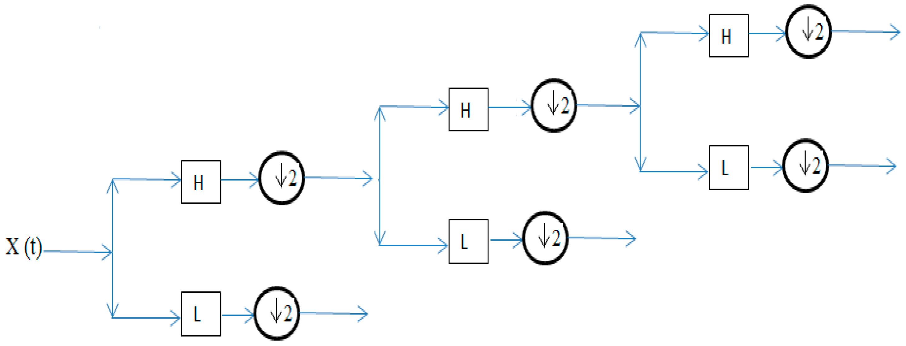
2. Wavelet Transform

One of the drawbacks in Fourier transform analysis is that frequency information can only be extracted for the complete duration of a signal [26]. Since the integral in the Fourier transform extends over all time, from $-\infty$. to $+\infty$, the information it provides is obtained from an average over the whole length of the signal [26]. To solve this problem, various techniques have been presented, such as short-time Fourier transform (STFT), Gabor transform, Wigner–Ville transform, and wavelet transform. Among these techniques, wavelet transform was identified as an effective method. In general, the wavelet function is defined as follows [8]:

$$\psi (t)=g(t)e^{-j2\pi f_{0}t}$$

(1)

$\psi (t)$ is an oscillatory time-dependent function which depends on two variables $(\tau ,a)$. The function on the time axis is transmitted with a change in $(\tau )$ and the width of function $\psi (t)$ on the time axis is changed with a change in the scale $(a)$. In the case of $a<1$, $\psi (t)$ is transformed to $\psi (t/a)$ and extended, and its frequency should be reduced. If $a<1$, the function is more compact, and its frequency is increased. The wavelet transform of a function is obtained from the following equation [8]:

$$w_x(\tau ,a)={\displaystyle \underset{-\infty }{\overset{+\infty }{\int }}\frac{1}{\sqrt{a}}x(t){\psi }^{*}(\frac{t-\tau }{a}})dt$$

(2)

The properties of wavelet transform are as follows:

A)

The integral of the wavelet function is equal to zero in the time domain.

$${\displaystyle \underset{-\infty }{\overset{+\infty }{\int }}\psi (t)dt=0}$$

In other words, the mean value of $\psi (t)$ is zero.

$${\displaystyle \underset{-\infty }{\overset{+\infty }{\int }}\frac{{\left|\widehat{\mathsf{\psi }}(f)\right|}^2}{\left|f\right|}df<\infty }$$

B)

In addition, one of the following conditions exists:

$$\widehat{\mathsf{\psi }}(f)=0\hspace{1em}\hspace{1em}f\le 0$$

(3)

$$\widehat{\mathsf{\psi }}(f)=0\hspace{1em}\hspace{1em}f\ge 0$$

(4)

$${\displaystyle \underset{-\infty }{\overset{0}{\int }}\frac{{\left|\widehat{\mathsf{\psi }}(f)\right|}^2}{\left|f\right|}df}={\displaystyle \underset{0}{\overset{+\infty }{\int }}\frac{{\left|\widehat{\mathsf{\psi }}(f)\right|}^2}{\left|f\right|}df}$$

(5)

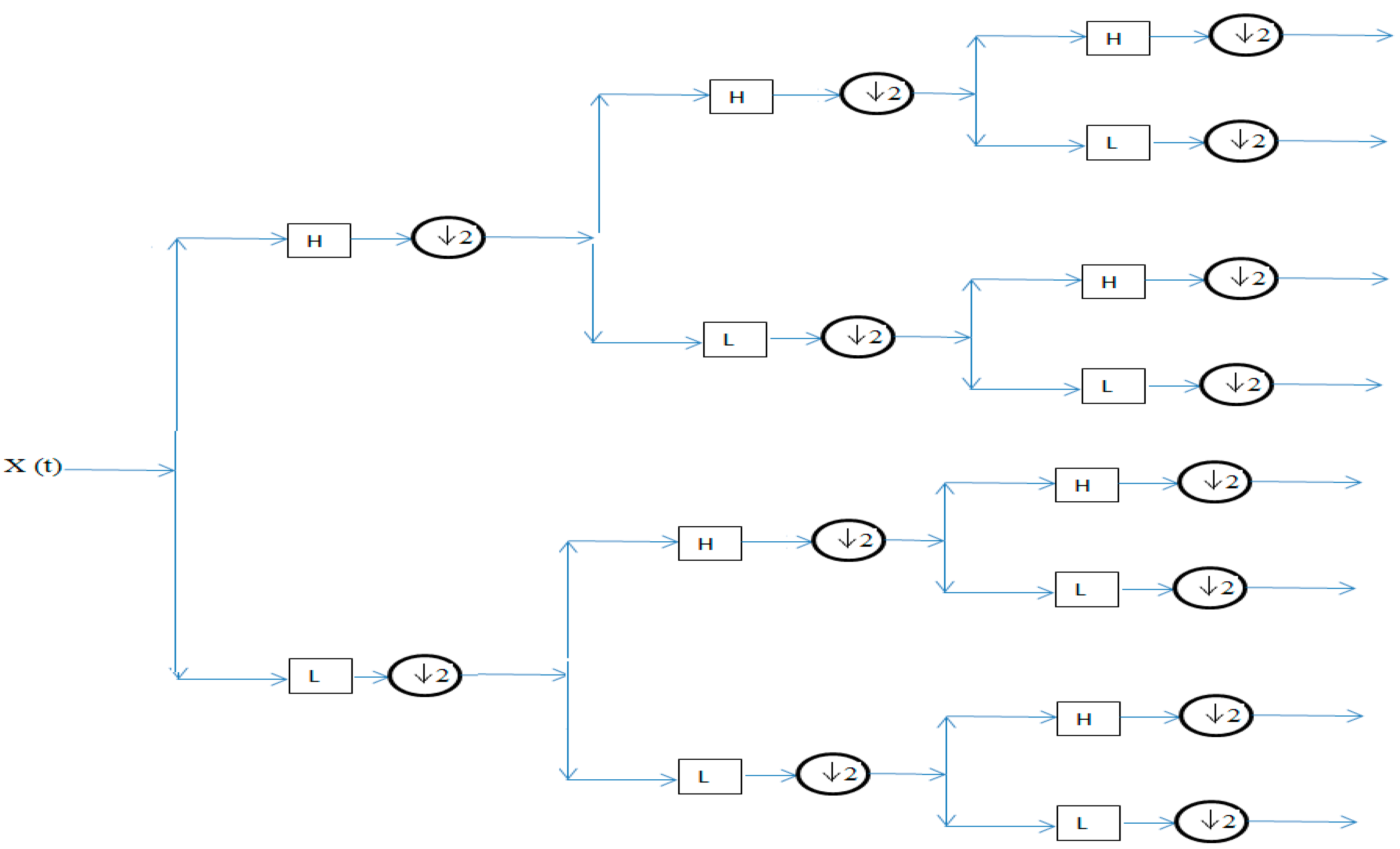
3. Multi-Resolution Analysis

The multi-resolution analysis algorithm was originally presented by Mallat [27]. In this analysis, the frequency resolution can be increased using a filter bank and thus is very effective in multi-resolution analysis. In the multi-resolution algorithm, considering the sampling frequency as Fs, the frequency domain resolution can be doubled using one low-pass and one high-pass filter. Accordingly, the resolution can then be increased by increasing the levels of decomposition. There are two methods for multi-resolution analysis—discrete wavelet transform (DWT) and discrete wavelet packet transform (DWPT). As shown in Figure 1, the first method (DWT) has a focus on lower frequencies. However, in the second method (DWPT), as shown in Figure 2, the resolution was improved significantly compared to the DWT using both low- and high-frequency filters [25,27]. In Figure 1 and Figure 2, H and L indicate the high-pass and low-pass filters. When the signal is decomposed at the third level, it is divided into eight frequency bands. When the sampling frequency is 12 kHz, the frequency bands at the third level of decomposition are presented as shown in

Table 1. The frequency intervals corresponding to the decomposition of a signal at the third level (Fs = 12,000 Hz).

Frequency Range (Hz)	Frequency Bands	Frequency Range (Hz)	Frequency Bands
(3000–3750)	Freq Band 5	(0–750)	Freq Band 1
(3750–4500)	Freq Band 6	(750–1500)	Freq Band 2
(4500–5250)	Freq Band 7	(1500–2250)	Freq Band 3
(5250–6000)	Freq Band 8	(2250–3000)	Freq Band 4

. When the signal is at the fourth level of decomposition, the signal is divided into 16 frequency bands. When the sampling frequency is 12 kHz and the signal is decomposed at the fourth level, the frequency bands at the fourth level of decomposition are presented as shown in

Table 2. The frequency intervals corresponding to the decomposition of a signal at the fourth level (Fs = 12,000 Hz).

Frequency Range (Hz)	Frequency Bands	Frequency Range (Hz)	Frequency Bands
(3000–3375)	Freq Band 9	(0–375)	Freq Band 1
(3375–3750)	Freq Band 10	(375–750)	Freq Band 2
(3750–4125)	Freq Band 11	(750–1125)	Freq Band 3
(4125–4500)	Freq Band 12	(1125–1500)	Freq Band 4
(4500–4875)	Freq Band 13	(1500–1875)	Freq Band 5
(4875–5250)	Freq Band 14	(1875–2250)	Freq Band 6
(5250–5625)	Freq Band 15	(2250–2625)	Freq Band 7
(5625–6000)	Freq Band 16	(2625–3000)	Freq Band 8

.

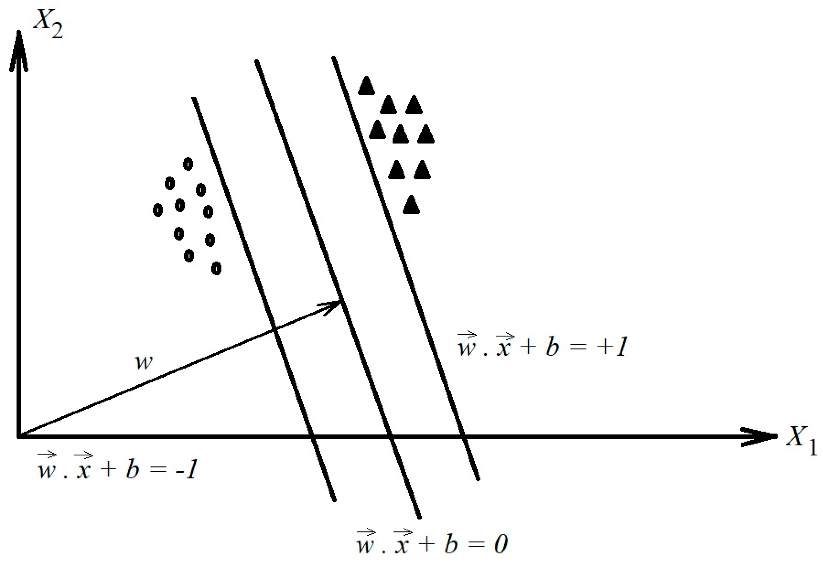
4. Support Vector Machine (SVM) Technique

The support vector machine classification method is based on the maximum distance between the data sets. This method was originally introduced in 1998 by Vapnik and Cortes [28]. In this method, the data were classified into two classes: $y_i=+1$ and $y_i=-1$. In this study, the aim was to check two classes of problems related to hard-margin support vector machines and soft-margin support vector machines. If the data could be linearly classified in the feature space, the classification was called hard-margin support vector machine classification (see Figure 3).

When the data were not linearly separable, the space of the data was transferred to a higher order space. In this case, data were linearly classified using support vector machines with soft-margins. If all of the data were considered as a pair of data points, such as $\left(x_1,y_1\right) , \left(x_2,y_2\right) , \dots , \left(x_n,y_n\right)$ where $x_n\in R^m , y_n\in \left\{-1,1\right\}$, then to classify the second order linear problems, the data were separated as follows:

$$w^T{x}_i+b\ge 1 \mathrm{for} y_i=+1$$

$$w^T{x}_i+b\le -1 \mathrm{for} y_i=-1$$

where b is the bias. The distance between the support vectors is obtained as follows:

$$d=\frac{2}{\Vert w\Vert }$$

where w is the normal vector perpendicular to the line $\overrightarrow{w}.\overrightarrow{x}+b=0$. and ‖w‖ is the magnitude of w. As the magnitude of d increases, the separation of variables will be more efficient. To increase the magnitude of d, the magnitude of w should decrease. Using the Lagrange function, the desired result (i.e., large d and small w parameters) can be defined:

$$L(w,b,\alpha )=\frac{{\Vert w\Vert }^2}{2}-{\displaystyle \sum _{i=1}^l{\alpha }_i.\{y_i.[(w,x_i)+b]-1\}}$$

(6)

where $({\alpha }_i)$ is the Lagrange coefficient. To solve the Lagrange equation, $({\alpha }_i)$ should be a maximum and $(d,w)$ should be a minimum:

$$\frac{\partial L(w,b,\alpha )}{\partial w}=0$$

(7)

$$\frac{\partial L(w,b,\alpha )}{\partial b}=0$$

(8)

After solving Equations (6)–(8), Equations (9) and (10) are obtained as follows:

$${\alpha }_i\{y_i(w^T{x}_i+b)-1\}=0\mathrm{for}i=1,2,3,\dots ,M$$

(9)

$${\alpha }_i\{y_i(w^T{x}_i+b)-1\}=0\mathrm{for}i=1,2,3,\dots ,M$$

(10)

In Equation (9), if ${\alpha }_i\ne 0$, then the training data $(x_i)$ are known as the support vectors. In this case the optimal separating hyperplane (OSH) is determined as follows:

$$w={\displaystyle \sum _{i=1}^l{\alpha }_i.y_i.x_i,}{\alpha }_i\ge 0,i=1,2,3,\dots ,\ell$$

(11)

where:

$${\displaystyle \sum _{i=1}^{\ell }{\alpha }_i.y_i=0},{\alpha }_i\ge 0,i=1,2,3,\dots ,\ell$$

If s is defined as $s=\left\{i|0<{\alpha }_i<c\right\}$, then from Equations (9) and (11): $b=\frac{1}{\left|s\right|}{{\displaystyle \sum }}_{i\in s}\left(y_i-w^T{x}_i\right)$. The distance of each point $(x_i)$ from the optimal separating hyperplane (OSH) is calculated as follows:

$$d(w,b,x)=\frac{\left|w.x+b\right|}{\Vert w\Vert }$$

(12)

Substituting Equation (11) into Equation (12), we obtain:

$$d(x)=\frac{({\displaystyle \sum _{i=1}^{\ell }{\alpha }_i.y_i.x_i).x+b}}{\Vert {\displaystyle \sum _{i=1}^{\ell }{\alpha }_i.y_i.x_i}\Vert }$$

(13)

The sign of $d(x)$ in Equation (13) shows the class of $x(i)$. If $d(x)>0$, the data will be categorized as class 1; if $d(x)<0$, the data will be categorized as class 2; and if $d(x)=0$, then $x(i)$ is on the border and cannot be classified. Here $\left|d\right|$ determines the distance between $x(i)$ and the optimal separating hyperplane (OSH). As the value of $\left|d\right|$ increases, the classification will be more efficient.

When the data are nonlinearly distributed, linear separation is not an effective method. In such cases, data will be transferred to a higher order space to be classified using a linear technique. This transformation will be done using the $\phi (x)$ operator rather than $x(i)$, where:

$$f(x)=w.\phi (x)+b$$

(14)

Substituting Equation (11) into Equation (14), the above equation can be generalized as follows:

$$f(x)={\displaystyle \sum _{i=1}^{\ell }{\alpha }_i.y_i.(\phi (x_i).}\phi (x))+b$$

(15)

In mapping to a higher order space, the $(\phi (x)\times \phi (x_i))$ should be selected appropriately. For this reason, the kernel function is defined as:

$$k(x_i,x)=(\varphi (x_i)\times \varphi (x))$$

The most commonly used kernel function is defined as follows:

A)

a polynomial kernel function:

$$k(x_i,x)={(x_i.x+1)}^p$$

(16)

B)

an RBF kernel function:

$$k(x_i,x)=\exp [-\gamma {\Vert x-x_i\Vert }^2]$$

(17)

More details about the SVM and classification problems can be found in References [12,13,14].

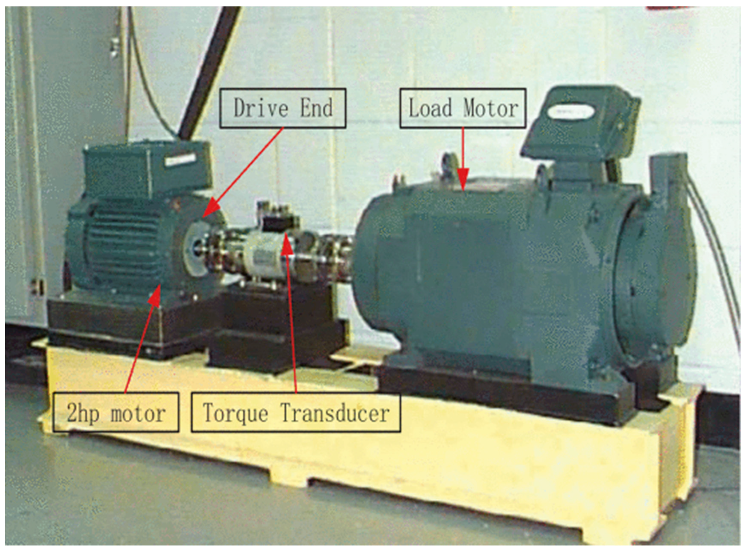
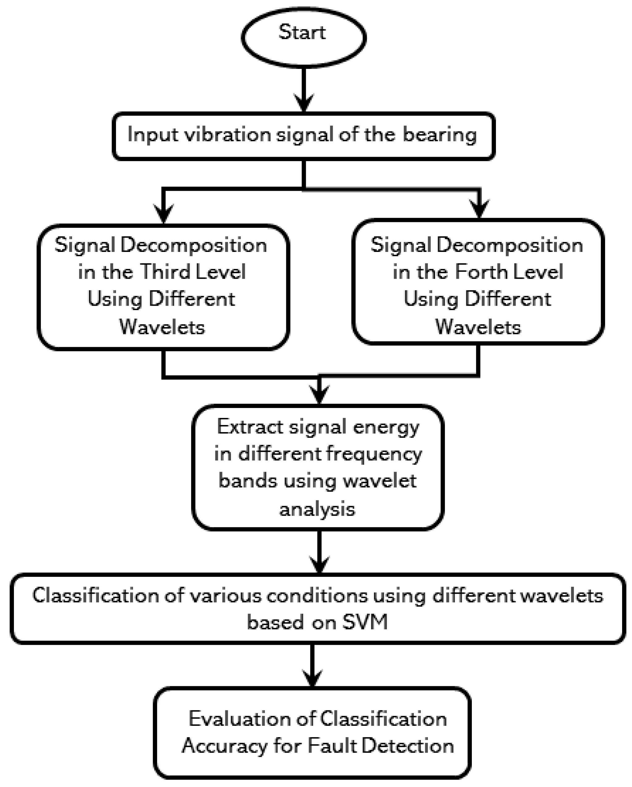
5. Data Acquisition of Vibration Signals

In this paper, the vibration signals of rolling bearing model 6205-2 RS JEM SKF deep-groove were obtained from the Case Western Reserve University Bearing Data Center [29]. For experimentation, an electrical motor connected to a fan was used to extract the signals for the bearings fault detection (Figure 4).

Signals used in this article consisted of different types of bearing operational conditions. These included: Normal operation conditions, the presence of faults in the inner ring, faults in the outer ring, and faults in the balls under different loads and rotational speeds. The sampling frequency was designated to be 12 kHz throughout the experiment, and the signals were obtained by an accelerometer placed perpendicular to the shaft. The experimental data acquired consisted of four vibrational signals for normal conditions and eight vibrational signals related to the faults in the inner ring, outer ring, and balls, totaling 28 vibration signals for the analysis in this study. Figure 5 shows the flowchart of the proposed method for the intelligent fault diagnosis of bearings based on energy levels in frequency bands using wavelet and support vector machines (SVM).

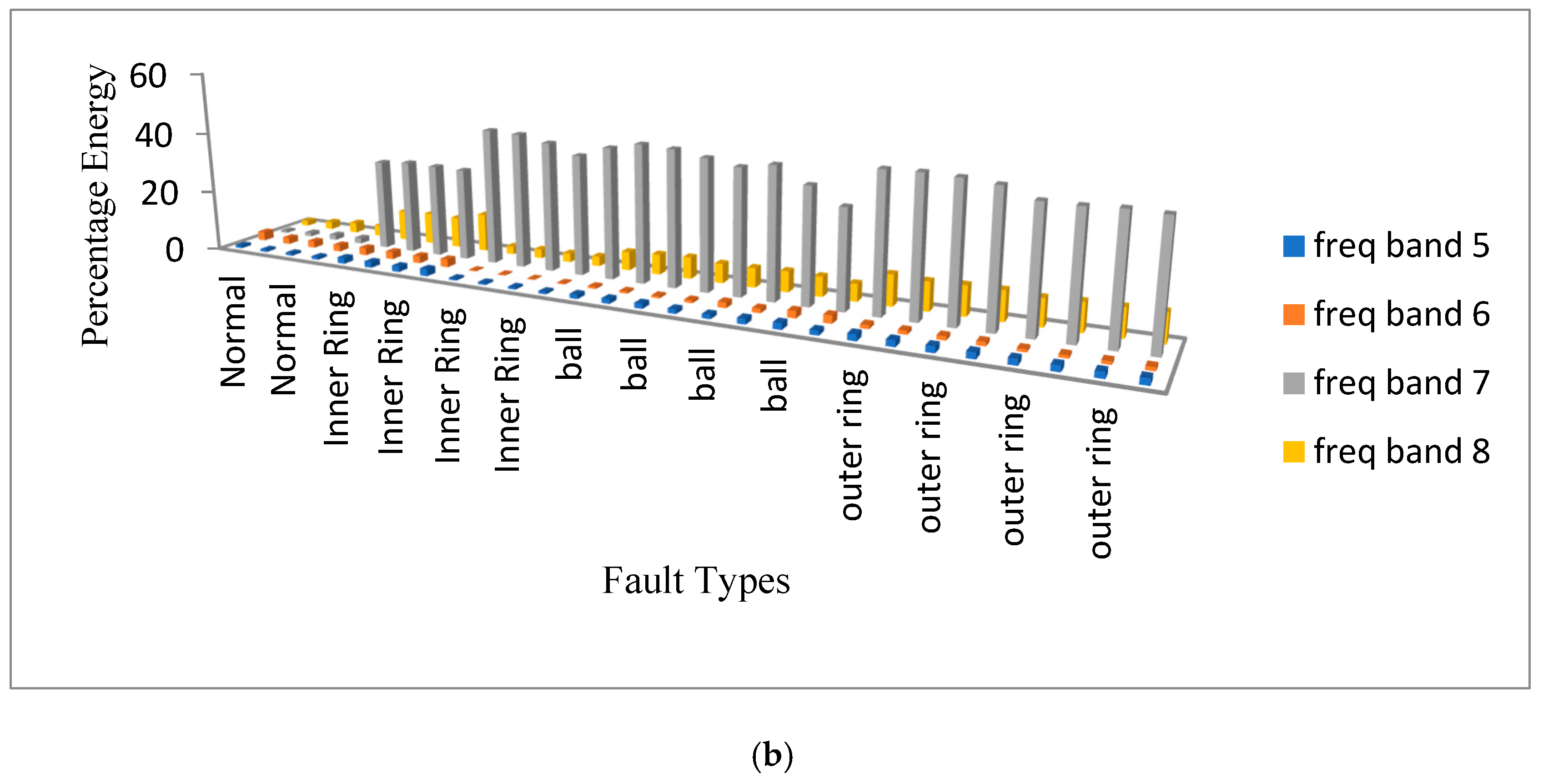
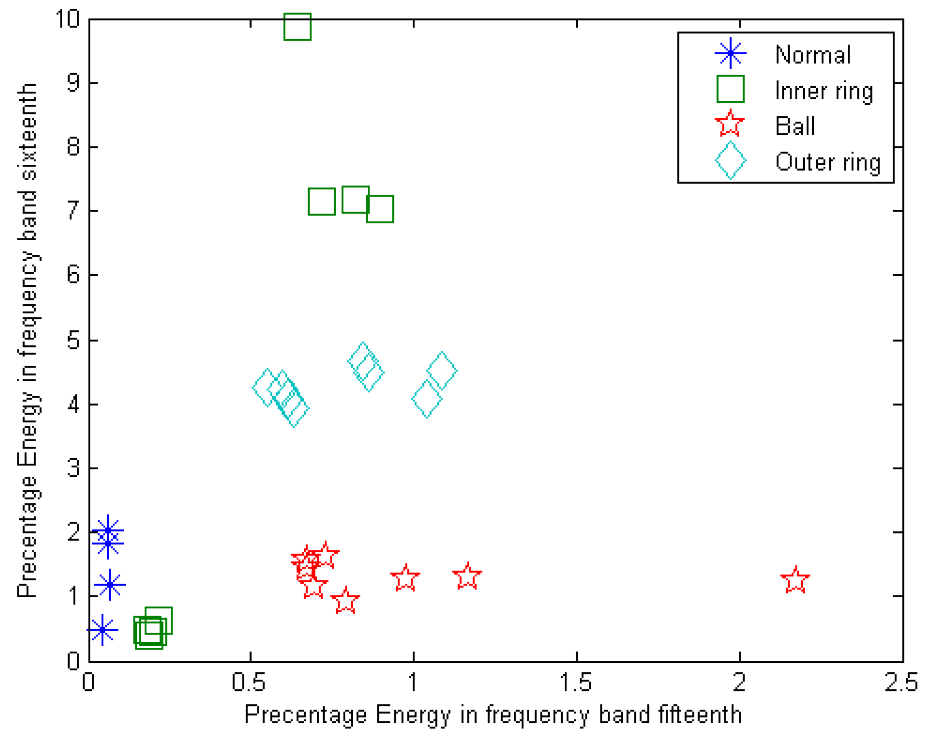
6. Feature Extraction

Feature extraction is the pivotal part of an intelligent fault diagnosis system. There are a variety of statistical methods for feature extraction from a signal [6,9,10]. The novel method presented in this study is based on the analysis of signal energy in different frequency bands using wavelet analysis.

Table 3. Energy extraction as signal energy by different wavelets.

Wavelet Type	Normal Conditions	Inner Ring	Outer Ring	Balls	Wavelet Type	Normal Conditions	Inner Ring	Outer Ring	Balls
Db (1–10)	2157.11	19,367.78	11,358.25	2200.625	bior 5.5	1646.074	19,875.59	14,148.54	2582.225
Sym (2–8)	2157.12	19,368.15	11,358.69	2200.63	bior 6.8	2220.009	19,964.09	11,197.79	2189.105
Coif (1–5)	2157.13	19,368.43	11,358.56	2200.65	rbio 1.1	2157.112	19,367.79	11,358.25	2200.554
dmey	2158.01	19,383.33	11,362.88	2202.375	rbio 1.3	1968.818	19,517.14	12,327.03	2327.723
bior 1.1	2157.112	19,367.79	11,358.25	2200.554	rbio 1.5	1928.785	19,601.41	12,917.27	2416.57
bior 1.3	2471.467	19,652.07	10,742.81	2132.575	rbio 2.2	2080.56	23,640.36	14,581.46	2763.02
bior 1.5	2627.541	19,954.79	10,477.61	2095.307	rbio 2.4	1834.783	23,242.51	15,360.39	2873.272
bior 2.2	2697.638	23,563.8	12,754.69	2561.615	rbio 2.6	1742.075	23,080.8	16,037.67	2982.819
bior 2.4	2844.135	23,600.42	11,734.45	2419.893	rbio 2.8	1697.09	23,004.08	16,639.32	3083.27
bior 2.6	2954.414	23,842.13	11,182.01	2329.608	rbio 3.1	3709.718	40,385.17	22,977.3	4467.429
bior 2.8	3039.554	24,100.1	10,784.85	2260.565	rbio 3.3	2278.809	37,702.51	23,492.65	4455.607
bior 3.1	3986.502	45,741.43	28,792.2	5301.835	rbio 3.5	1890.008	36,741.06	24,388.36	4596.692
bior3.3	3767.156	38,241.26	19,187.21	3980.502	rbio 3.7	1710.69	36,158.9	25,240.45	4744.515
bior 3.5	3768.738	37,900.59	17,383.33	3708.362	rbio 3.9	1617.109	35,760.62	26,009.97	4884.884
bior 3.7	3832.379	38,021.93	16,253.48	3519.478	rbio 4.4	2321.09	20,025.55	11,591.45	2264.359
bior 3.9	3902.459	38,245.49	15,448.34	3372.755	rbio 5.5	3175.766	20,351.78	9854.393	2047.906
bior 4.4	2050.796	20,143.06	11,956.86	2298.285	rbio 6.8	2104.933	19,875.52	12041.18	2326.006

presents the total energy of vibration signals in different conditions, using different wavelets. As shown in Table 3, different wavelets were used for decomposition in the third level for signal feature extraction. For a better understanding of the process in Table 3, these data are presented as a graph in Figure 6.

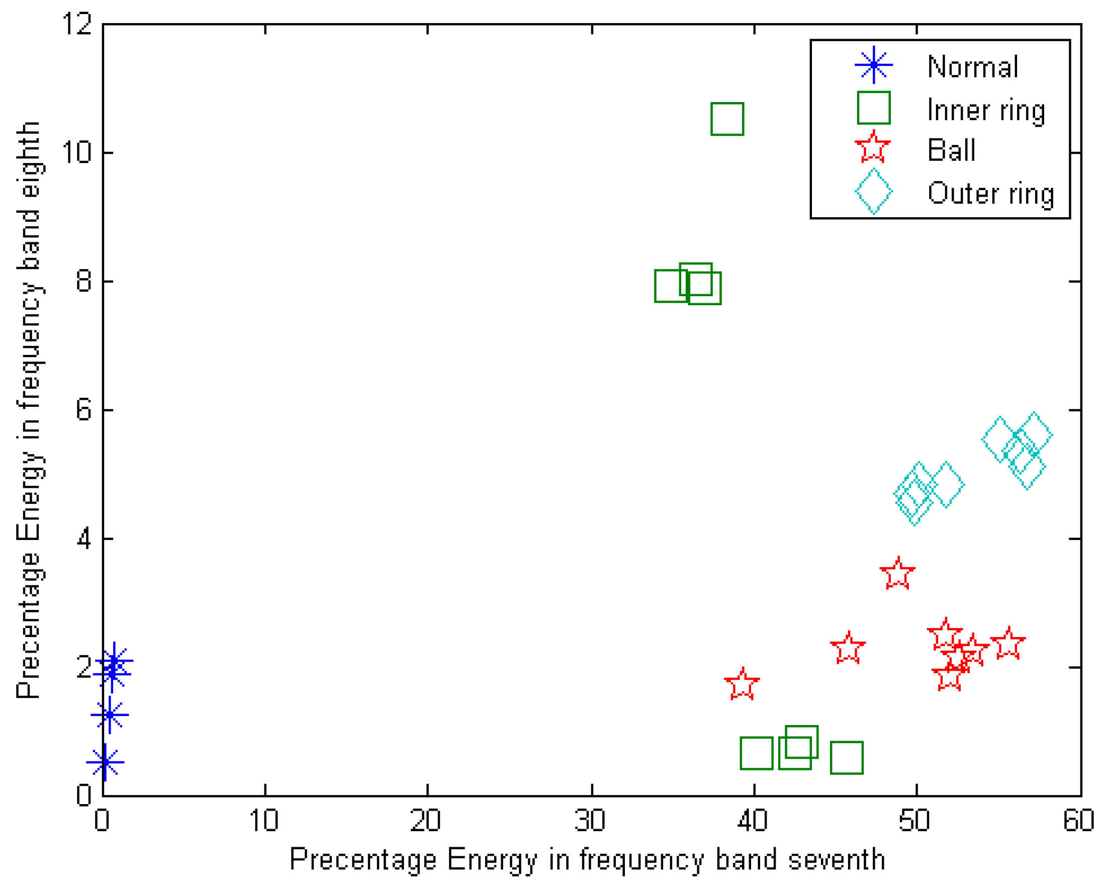
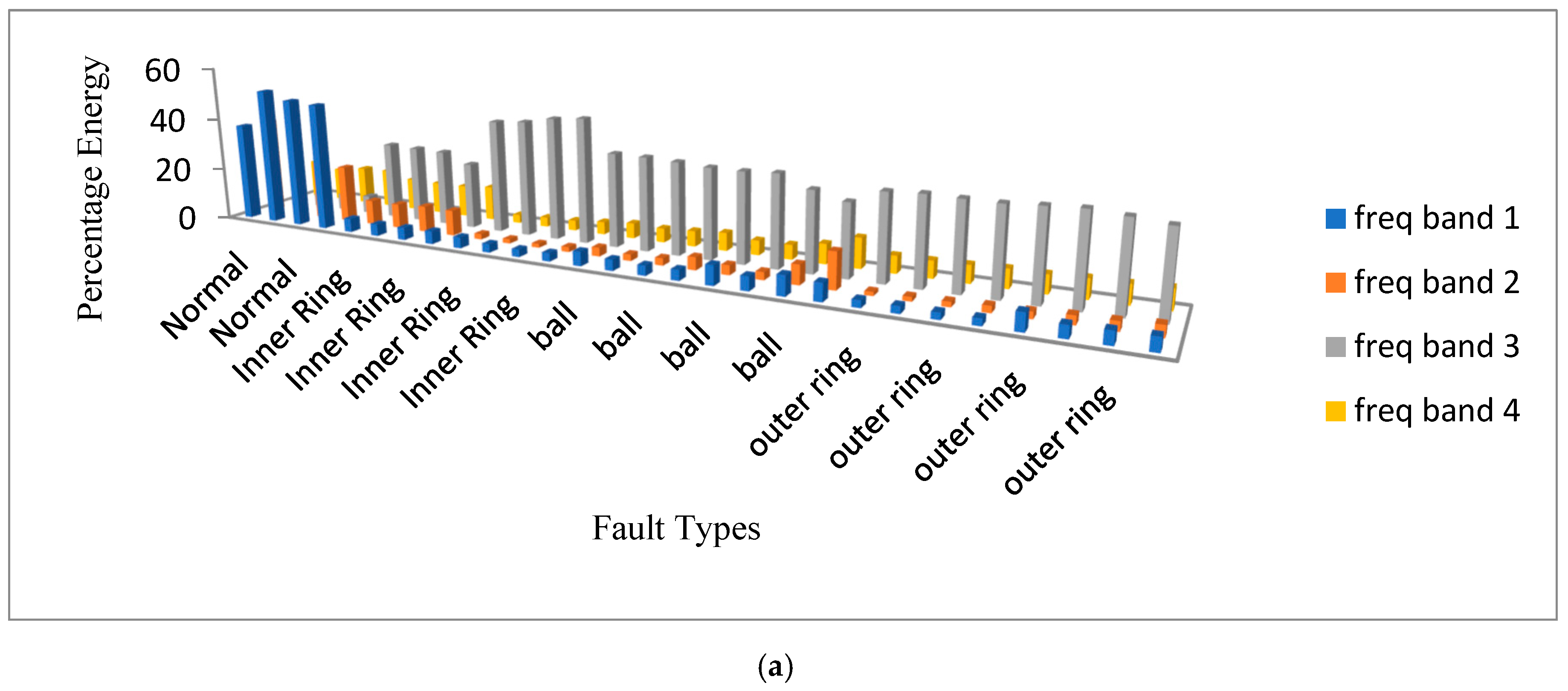
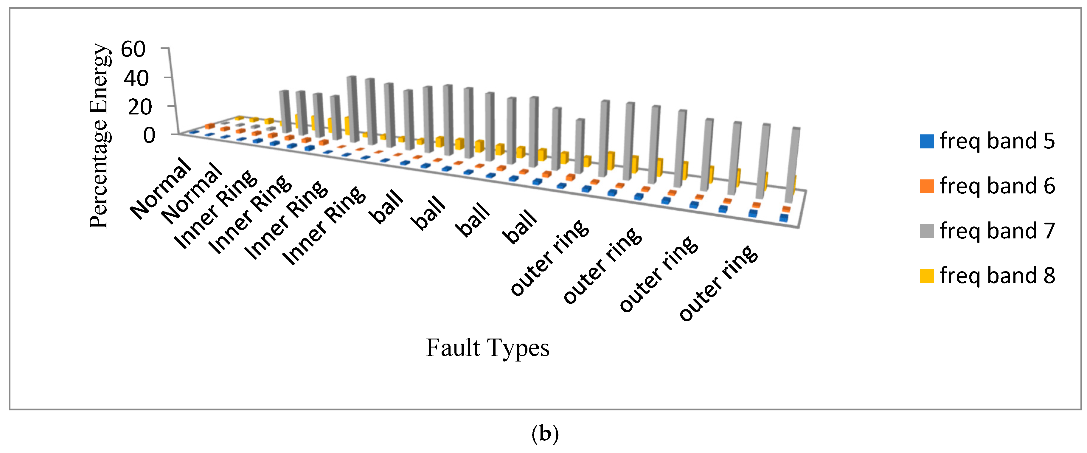
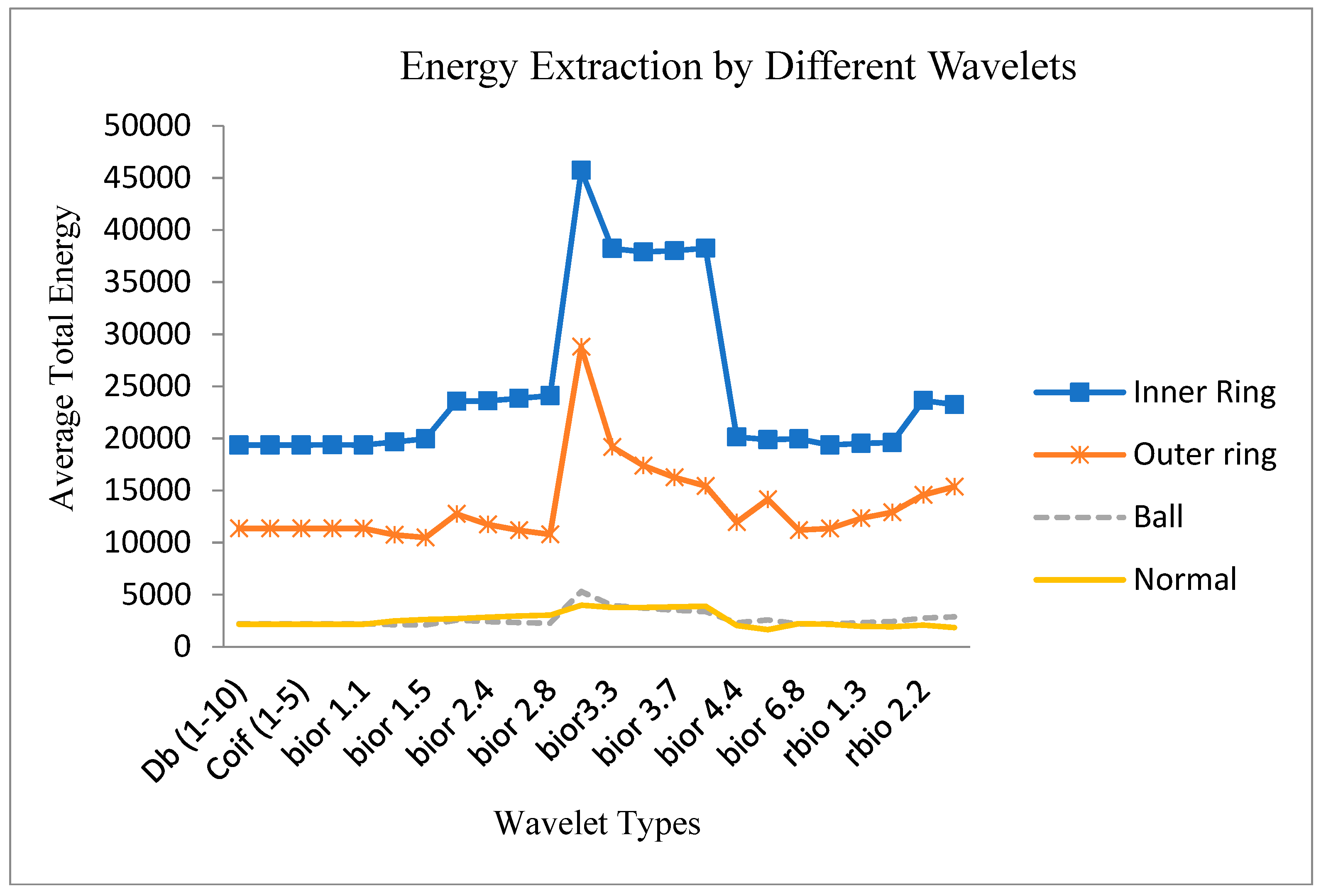
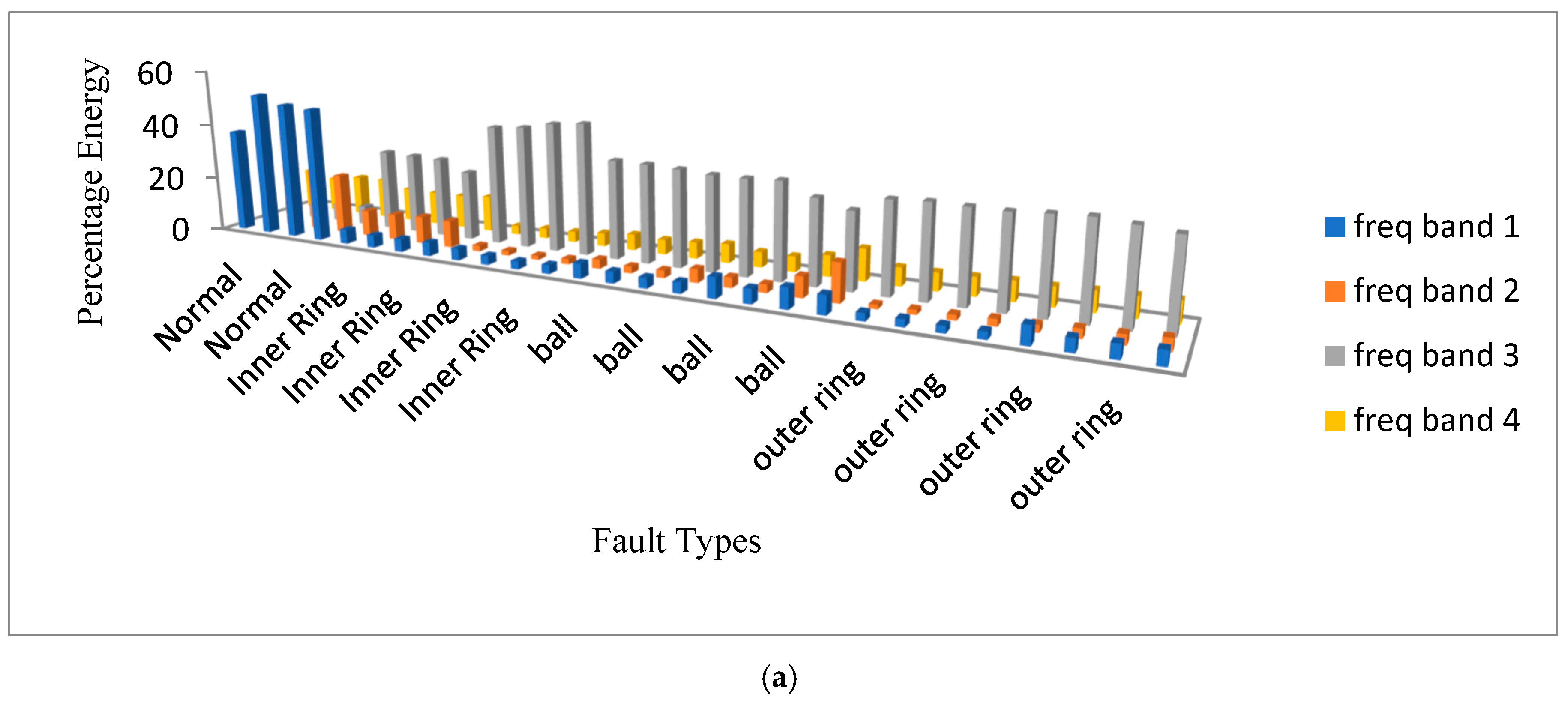
7. Signal Decomposition in the Third Level Using Different Wavelets

In this section, signals were decomposed by wavelets in the third level. Hence, there were eight (2^3 = 8) frequency bands. Following the signal decomposition, the evaluation of the signal’s energy in each frequency band identified the faults in the inner ring, outer ring, and balls. Figure 7 shows the energy level of each frequency band for the decomposition by wavelet db1 at the third level.

As can be seen in Figure 7, for the signals in normal conditions, the larger portion of the energy was in the first and second frequency bands. However, in case of the faults in the inner ring, outer ring, and balls, the larger portion of the energy was in the third and seventh frequency bands. Since there were appropriate and significant changes in the seventh and eighth frequency bands, these two bands were selected as feature vectors (identifiers). It should be noted that the more variation that exists between the energy levels of each type of fault, the better the detection and diagnosis will be (Figure 8).

Figure 9 shows the graphical classification of the different bearing conditions using energy levels in the seventh and eighth frequency bands in the third level. In Figure 9, the horizontal and vertical axes correspond to the energy level in the seventh and eighth frequency bands, respectively. The rate of change of energy in the seventh and eighth frequency bands are directly dependent on the type of wavelets. Hence, it is necessary to evaluate different kinds of wavelets to determine the appropriate wavelet type for classification. As presented in Table 3, three kinds of wavelets from the Daubechies wavelet group were used for signal decomposition in the third level in the seventh and eighth frequency bands. Table 3 shows that the decomposition and classification of the signals strongly depend on the type of wavelet.

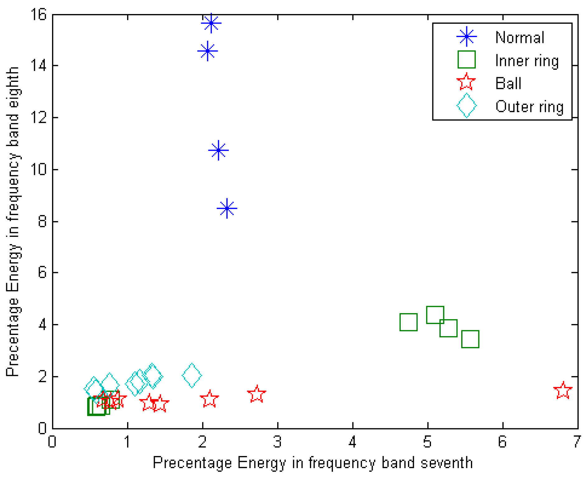
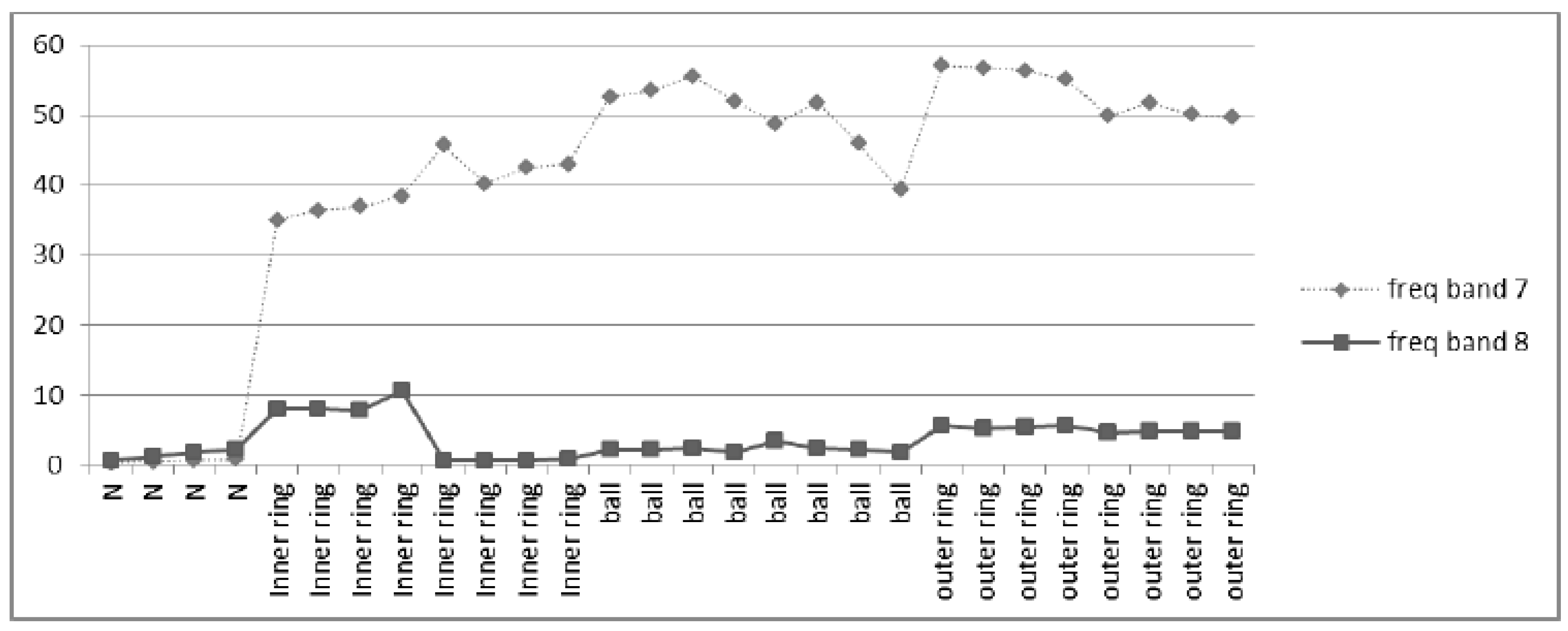
8. Signal Decomposition in the Fourth Level Using Different Wavelets

Similar to the previous section for feature extraction, these signals were decomposed by wavelets in the fourth level. In this case, 16 frequency bands exist (2^4 = 16). Following the signal decomposition, the energy level in each frequency band for normal conditions, as well as faults in the inner ring, outer ring, and balls were achieved. Figure 10 shows the energy level of different frequency bands using wavelet db3 with the fourth level of decomposition.

Figure 11 shows the graphical classification of the different bearing conditions using energy levels in the seventh and eighth frequency bands in the fourth level. As seen in Figure 11, the seventh and eighth frequency bands were not suitable to select the feature vectors, because changes in these two frequency bands were close together. However, choosing frequency bands 15 and 16 remarkably increased the accuracy of classification due to the larger changes of energy in these frequency bands. This is because there were 16 frequency bands in the fourth level of decomposition, while there were only eight frequency bands in the third level. Thus, in the third level of decomposition, the variation of energy levels in the seventh and eighth frequency bands was very low and close to each other. Figure 11 and Figure 12 as well as

Table 4. Classification accuracy of various conditions using different wavelets based on support vector machine (SVM) (analysis was performed in the third level and was used in the seventh and eighth frequency bands for data input to the SVM).

Wavelet Type	Normal Conditions	Inner Ring	Outer Ring	Balls	Wavelet Type	Normal Conditions	Inner Ring	Outer Ring	Balls
Db1	100%	100%	100%	100%	Coif2	100%	92%	92%	100%
Db2	100%	92%	100%	92%	Coif3	100%	100%	92%	92%
Db3	100%	78%	100%	92%	bior 1.1	100%	100%	100%	100%
Sym2	100%	92%	100%	92%	bior 1.3	100%	92%	100%	100%
Sym3	100%	92%	100%	92%	bior 1.5	100%	71%	100%	100%
Sym4	100%	85%	100%	92%	rbio 1.1	100%	71%	100%	92%
Coif1	100%	78%	100%	92%	rbio 1.3	100%	100%	100%	92%

and

Table 5. Classification accuracy of various conditions using different wavelets based on support vector machine (SVM) (analysis was performed in the fourth level and was used in the seventh and eighth frequency bands for data input to the SVM).

Wavelet Type	Normal Conditions	Inner Ring	Outer Ring	Balls	Wavelet Type	Normal Conditions	Inner Ring	Outer Ring	Balls
Db1	85%	92%	100%	85%	Coif2	92%	78%	71%	64%
Db2	85%	92%	100%	92%	Coif3	85%	64%	64%	50%
Db3	100%	92%	92%	57%	bior 1.1	85%	92%	100%	85%
Sym2	85%	100%	100%	57%	bior 1.3	100%	78%	85%	42%
Sym3	100%	85%	100%	50%	bior 1.5	85%	85%	85%	64%
Sym4	100%	78%	100%	64%	rbio 1.1	92%	100%	100%	71%
Coif1	85%	85%	100%	85%	rbio 1.3	85%	78%	100%	78%

show the accuracy in classification for the selected feature vectors in the different frequency bands. Classification accuracy for different types of faults depends on the level of decomposition and the determined level of signal energy using different wavelets. Since each type of wavelet has different characteristics influencing the decomposition of the signal, and they were used to detect all types of defects, the accuracy of classification could be different (or lower in some cases) due to the characteristics of the particular wavelet used for the classification of different faults.

As shown in Table 1 and Table 2, the bandwidth of the seventh and eighth frequency bands in the third level of decomposition was equal to the total (sum) bandwidth for the 13th to 16th frequency bands in the fourth level of decomposition. Since most of the variations in the signals in this study occurred in the 9000–12,000 Hz frequency range, to analyze the variations in the fourth level of decomposition, the 14th to 16th frequency bands should be evaluated. This is the main reason for the classification error when using the seventh and eighth frequency bands at the fourth level of decomposition. Due to the highest variation in fault detection, bior and rbior wavelet groups were the most adequate type of wavelets for real applications.

9. Conclusions

The proposed decomposition technique based on wavelet and SVM successfully detected and classified the faults in bearings with a high level of accuracy. The effectiveness of the proposed feature selection and classification method was also demonstrated by the testing results. The accuracy of the classification and detection in this method strongly depended on the type of wavelet selected for the decomposition. Higher similarity between the selected wavelet and the original signal resulted in a higher level of energy in different frequency bands. The outcome of the proposed method is summarized as follows: Total minimum average energy levels of the signal occurred in normal conditions, followed by the presence of faults in the balls. Total maximum average energy levels of signals occurred under fault conditions in the inner ring and outer ring. For the vibration signals of the faults in the inner ring or outer ring, the most variation occurred in the bior and rbior wavelet groups. The seventh and eighth frequency bands were a good choice of feature vectors when the third decomposition level was used. The 15th and 16th frequency bands were good for choosing feature vectors when the fourth decomposition level was used. If the seventh and eighth frequency bands in the fourth decomposition level were used, the classification error was significant.

References

1. Liu, J.; Shao, Y. Overview of dynamic modelling and analysis of rolling element bearings with localized and distributed faults. Nonlinear Dyn. 2018, 93, 1765–1798. [Google Scholar] [CrossRef]
2. Mehrabi, A.B.; Farhangdoust, S. A Laser-Based Non-Contact Vibration Technique for Health Monitoring of Structral Cables: Background, Success, and New Developments. Adv. Acoust. Vib. 2018, 2018, 1–13. [Google Scholar]
3. Lim, T.C.; Singh, R. Vibration transmission through rolling element bearings, part IV: Statistical energy analysis. J. Sound Vib. 1992, 153, 37–50. [Google Scholar] [CrossRef]
4. Martin, H.R.; Honarvar, F. Application of statistical moments to bearing failure detection. Appl. Acoust. 1995, 44, 67–77. [Google Scholar] [CrossRef]
5. Parey, A.; el Badaoui, M.; Guillet, F.; Tandon, N. Dynamic modelling of spur gear pair and application of empirical mode decomposition-based statistical analysis for early detection of localized tooth defect. J. Sound Vib. 2006, 294, 547–561. [Google Scholar] [CrossRef]
6. Antoni, J. Cyclic spectral analysis of rolling-element bearing signals: Facts and fictions. J. Sound Vib. 2007, 304, 497–529. [Google Scholar] [CrossRef]
7. Chebil, J.; Noel, G.; Mesbah, M.; Deriche, M. Wavelet Decomposition for the Detection and Diagnosis of Faults in Rolling Element Bearings. Jordan J. Mech. Ind. Eng. 2009, 3, 260–267. [Google Scholar]
8. Tang, Y.Y. Wavelet Theory and Its Application to Pattern Recognition, 2nd ed.; World Scientific Publishing Co., Inc.: River Edge, NJ, USA, 2009. [Google Scholar]
9. Li, Z.; Feng, Z.; Chu, F. A load identification method based on wavelet multi-resolution analysis. J. Sound Vib. 2014, 333, 381–391. [Google Scholar] [CrossRef]
10. He, Q.; Wang, X. Time–frequency manifold correlation matching for periodic fault identification in rotating machines. J. Sound Vib. 2013, 332, 2611–2626. [Google Scholar] [CrossRef]
11. Lin, J.; Qu, L. Feature extraction based on morlet wavelet and its application for mechanical fault diagnosis. J. Sound Vib. 2000, 234, 135–148. [Google Scholar] [CrossRef]
12. Nikravesh, S.M.Y.; Taheri, H.; Wagstaff, P. Identification of Appropriate Wavelet for Vibration Study of Mechanical Impacts. In Proceedings of the ASME 2013 International Mechanical Engineering Congress and Exposition, San Diego, CA, USA, 15–21 November 2013; Volume 14, p. V014T15A022. [Google Scholar]
13. Nikravesh, S.M.Y.; Taheri, H. Onset of Nucleate Boiling Detection in a Boiler Tube by Wavelet Transformation of Vibration Signals. J. Nondestruct. Eval. Diagn. Progn. Eng. Syst. 2018, 1, 31005–31007. [Google Scholar]
14. Liu, X.; Bo, L.; He, X.; Veidt, M. Application of correlation matching for automatic bearing fault diagnosis. J. Sound Vib. 2012, 331, 5838–5852. [Google Scholar] [CrossRef]
15. Peng, Z.K.; Tse, P.W.; Chu, F.L. An improved Hilbert–Huang transform and its application in vibration signal analysis. J. Sound Vib. 2005, 286, 187–205. [Google Scholar] [CrossRef]
16. Li, J.; Chen, X.; He, Z. Multi-stable stochastic resonance and its application research on mechanical fault diagnosis. J. Sound Vib. 2013, 332, 5999–6015. [Google Scholar] [CrossRef]
17. Liu, J.; Xu, Z.; Zhou, L.; Nian, Y.; Shao, Y. A statistical feature investigation of the spalling propagation assessment for a ball bearing. Mech. Mach. Theory 2019, 131, 336–350. [Google Scholar] [CrossRef]
18. Lu, W.; Jiang, W.; Yuan, G.; Yan, L. A gearbox fault diagnosis scheme based on near-field acoustic holography and spatial distribution features of sound field. J. Sound Vib. 2013, 332, 2593–2610. [Google Scholar] [CrossRef]
19. Kar, C.; Mohanty, A.R. Vibration and current transient monitoring for gearbox fault detection using multiresolution Fourier transform. J. Sound Vib. 2008, 311, 109–132. [Google Scholar] [CrossRef]
20. Nikravesh, S.M.Y.; Chegini, S.N. Crack identification in double-cracked plates using wavelet analysis. Meccanica 2013, 48, 2075–2098. [Google Scholar] [CrossRef]
21. Li, B.; Chen, X.F.; Ma, J.X.; He, Z.J. Detection of crack location and size in structures using wavelet finite element methods. J. Sound Vib. 2005, 285, 767–782. [Google Scholar] [CrossRef]
22. Kim, E.-Y.; Lee, Y.-J.; Lee, S.-K. Heath monitoring of a glass transfer robot in the mass production line of liquid crystal display using abnormal operating sounds based on wavelet packet transform and artificial neural network. J. Sound Vib. 2012, 331, 3412–3427. [Google Scholar] [CrossRef]
23. Rucka, M.; Wilde, K. Application of continuous wavelet transform in vibration based damage detection method for beams and plates. J. Sound Vib. 2006, 297, 536–550. [Google Scholar] [CrossRef]
24. Rafiee, J.; Rafiee, M.A.; Tse, P.W. Application of mother wavelet functions for automatic gear and bearing fault diagnosis. Expert Syst. Appl. 2010, 37, 4568–4579. [Google Scholar] [CrossRef]
25. Liu, H.; Wang, J.; Lu, C. Rolling bearing fault detection based on the teager energy operator and elman neural network. Math. Probl. Eng. 2013, 2013, 10. [Google Scholar] [CrossRef]
26. Newland, D.E. An Introduction to Random Vibrations, Spectral & Wavelet Analysis, 3rd ed.; Dover Publications: New York, NY, USA, 1993. [Google Scholar]
27. Mallat, S.G. A Theory for Multiresolution Signal Decomposition. IEEE Trans. Pattern Anal. Mach. Intell. 1989, 11, 674–693. [Google Scholar] [CrossRef]
28. Cortes, C.; Vapnik, V. Supprot-Vector Networks. Mach. Learn. 1995, 297, 273–297. [Google Scholar] [CrossRef]
29. CWRU. Case Western Reserve University Bearing Data Center. Available online: http://www.eecs.case.edu/labratory/bearing/download.html (accessed on 4 December 2012).
Figure 1. Wavelet decomposition using discrete wavelet transform (DWT).
Jmmp 03 00011 g001
Figure 2. Wavelet decomposition using discrete wavelet packet transform (DWPT).
Jmmp 03 00011 g002
Figure 3. Schematic drawing showing the separation of the data.
Jmmp 03 00011 g003
Figure 4. Equipment and experimental setup to extract the vibration signals for the bearing fault diagnosis.
Jmmp 03 00011 g004
Figure 5. Flowchart of the proposed method for the intelligent fault diagnosis of bearings based on energy levels in frequency bands using wavelet and support vector machines (SVM).
Jmmp 03 00011 g005
Figure 6. Signal energy extracted by different wavelets for different fault conditions.
Jmmp 03 00011 g006
Figure 7. Percentage energy in the third level of decomposition by db3. (a) frequency bands 1–4, and (b) frequency bands 5–8.
Jmmp 03 00011 g007aJmmp 03 00011 g007b
Figure 8. Changes in the signal’s energy level in the seventh and eighth frequency bands.
Jmmp 03 00011 g008
Figure 9. Third level of decomposition by db3 (classification accuracy for four different conditions: normal = 100%, inner ring = 78%, outer ring = 100%, and balls = 92%).
Jmmp 03 00011 g009
Figure 10. Percentage of energy in the fourth level of decomposition by db3, (a) frequency bands 1–4, and (b) frequency bands 5–8.
Jmmp 03 00011 g010aJmmp 03 00011 g010b
Figure 11. The fourth level of decomposition by db3 (classification accuracy for four different conditions: normal = 100%, inner ring = 78%, outer ring = 100%, and balls = 92%).
Jmmp 03 00011 g011
Figure 12. The fourth level of decomposition by db3 (classification accuracy for four different conditions: normal = 100%, inner ring = 78%, outer ring = 100%, and balls = 92%).
Jmmp 03 00011 g012