MaskLenNet: A Query-Based Instance Segmentation and Length Prediction Network for Quantitative Industrial Tool Wear and Breakage Assessment

Abstract

Tool wear detection is essential for machining quality control and predictive maintenance, but conventional inspection is often manual, time-consuming, and operator-dependent. Existing learning-based visual methods still face challenges in jointly achieving reliable wear-type recognition, accurate wear-region localization, and quantitative wear-width measurement under shop-floor imaging conditions. To address these issues, this study proposes MaskLenNet, a query-based instance segmentation and length prediction network for solid carbide end-milling tool diagnosis. MaskLenNet combines a Swin Transformer backbone, query-based instance-mask prediction, wear-oriented attention, and a key-point head that directly estimates the maximum wear-land width (VB). Evaluation uses 234 images from 54 physical tools under a tool-disjoint split, so different rotations of one tool cannot occur in both training and evaluation sets. On the held-out test set, MaskLenNet achieves 96.52% matched-instance classification accuracy, 95.75% foreground instance mIoU, and a VB mean absolute error of 0.010214 mm. Relative to BEiT-Base, the gains are 3.04 and 3.60 percentage points in accuracy and mIoU, respectively. These results demonstrate promising performance within the evaluated acquisition system; they do not establish equivalence to microscopy or generalization to other machines, optics, workpiece materials, or sites.

1. Introduction

With the continuous innovation in science and technology, the intersection of traditional manufacturing and advanced AI technologies has sparked significant advancements, fueling confidence in the forthcoming era of intelligent industry [1]. In this era of digital manufacturing, computer numerical control (CNC) machines play a pivotal role, and cutting tools have a direct impact on machining quality [2]. Efficient and intelligent tool condition monitoring (TCM) is therefore crucial for enhancing production efficiency, maintaining dimensional accuracy, and supporting predictive maintenance [3]. This study focuses specifically on coated solid-carbide end mills used in end-milling operations.

Currently, research in tool condition monitoring predominantly focuses on indirect and direct methods [4]. Indirect methods assess tool wear by analyzing online sensor signals like current, acoustic emissions, and vibrations [5]. Despite their efficiency and accuracy, these methods heavily rely on sensors and signal processing technologies. However, noise disturbances continue to undermine signal transmission, posing a significant and unresolved challenge [6]. Direct methods primarily apply radiographic graphic measurement, resistance measurement, and machine vision to determine wear on the cutting edge’s surface [7]. Compared to indirect methods, direct methods are better suited for high-efficiency automated environments and offer higher detection accuracy. Additionally, direct methods monitor targets more directly than sensor-based indirect methods, enhancing reliability.

In recent years, a growing body of research has integrated machine vision with tool wear monitoring. Common image-processing techniques include segmentation, morphology, filtering, adaptive thresholding, and grayscale transformation. Agarwal et al. [8] combined Gaussian filtering and Otsu thresholding [9] to quantify wear area in milling tools. Shahabi and Ratnam [10] developed an online tool-tip wear system based on the difference between unworn and worn images, and later examined notch wear and built-up edge in turning tools [11,12]. These examples also show why the cutting process and workpiece material must be stated: continuous turning, interrupted end-milling, and stamping impose different combinations of thermal cycling, impact, abrasion, and adhesion. Likewise, steels of moderate hardness, hardened die steels, and difficult-to-cut alloys produce different dominant wear mechanisms and optical appearances [13].

Lachance et al. [14] developed the Fully Automated Surface Condition Analysis Tool (FASCAT) wear measurement system, which measures wear flats by capturing them optically. A total of 254 edge profile cutting head images make up the new dataset constructed by García-Ordás et al. [15]. This is the first adequately curated dataset available to the public. Bagga et al. [16] measured flank wear by using region segmentation and edge detection techniques. To evaluate the probability of low, medium, and high wear levels, Barreiro et al. [17] suggested an approach based on texture description and linear discriminant analysis. Ye et al. [18] separated the tool damage into areas that were broken and worn. Next, utilizing visual feature migration and state-of-the-art reconstruction, tool wear and breakage picture data were recovered, respectively. To address the impossibility of directly measuring the worn tool, Fernández-Robles et al. [19] processed and analyzed micro-tool pictures, providing useful information to estimate the evolution of tool wear.

Although the aforementioned methods achieve high testing accuracy in specific application scenarios, the limitations of traditional digital image processing in manual feature extraction, limited adaptability, and difficulty in coping with noise disturbances critically compromise their generalizability. Additionally, the need for manual parameter adjustments complicates the optimization of the network. Over the past ten years, there has been notable progress in machine learning approaches—specifically in deep learning (DL) methods—to tackle computer vision (CV) issues at a level that is comparable to or better than human performance [20]. Recent research has witnessed a surge in the application of convolutional neural networks (CNNs) for tool wear monitoring. These CNN-based approaches have demonstrated promising results, suggesting their immense potential as a valuable tool in this domain. Wang et al. [21] introduced a hybrid machine learning approach that combines recurrent neural networks (RNNs) and CNNs to integrate heterogeneous data for the prognosis of tool condition. In order to identify tool wear areas in microscopic pictures, Bergs et al. [22] suggested two methods: one for semantic segmentation and the other for tool type classification. Lin et al. [23] integrated object detection and image segmentation for detecting the tool wear area on stitched images, and they obtained the best maximum dice coefficient score with 0.93. Wu et al. [24] coupled traditional image processing with the U-Net [25] semantic segmentation network to extract features of tool wear areas; the prediction accuracy was only 17% less than the error of manual measurements.

Recent work further illustrates three complementary directions. Li et al. [26] directly quantified micro-milling wear from images and improved robustness to uneven illumination and arbitrary spindle orientation through image restoration, registration, and geometric wear extraction. Singh et al. [27] used a Vision Transformer for image-based wear recognition in end-milling of Inconel 718 and evaluated generalization under changed lighting, highlighting both the value of global self-attention and the need to test acquisition-domain shifts. Beyond direct imaging, Liu et al. [28] fused acoustic and force features for abrasive-belt wear recognition under variable grinding parameters; their cross-condition results reinforce that performance measured under fixed operating conditions should not be interpreted as operating-condition-independent generalization. These studies motivate the present combination of direct quantitative imaging, Transformer-based instance representation, and cautious within-domain evaluation.

While these deep learning-based techniques effectively address the limitations of conventional approaches by discovering the innate patterns and characteristics in images, leading to groundbreaking advancements in the field of image processing, they ignore the quantitative assessment of tool wear, making them inadequate in meeting the stringent requirements for accurate and reliable tool damage assessment in industrial applications. Driven by the recognition of quantitative tool wear evaluation’s pivotal role and extensive industrial applications, researchers have embarked on a surge of research in this domain, fueled by the advancements in deep learning segmentation techniques.

To address the challenge of tool wear detection in the stamping process, Schlegel et al. [29] proposed a tool wear segmentation method based on fully convolutional networks (FCNs) and digital image processing. This method enables pixel-level classification of different wear types, facilitating the spatial analysis of tool wear. Experimental results demonstrate that the model achieves high intersection over union (IoU) values for various tool wear categories, with an average IoU of 91.95% on the test set. Notably, it exhibits exceptional performance in background, no-wear area, and groove categories. While this method effectively classifies and quantitatively evaluates tool wear regions, it falls short in assessing wear extent and lacks modifications or innovations to the employed backbone network, making it difficult to adapt to different task scenarios. Li et al. [30] proposed an intelligent detection method based on the Segment Anything Model (SAM). Firstly, an initial image segmentation mask is generated using U-Net. Then, points of interest (PoIs) are obtained through binarization processing. These PoIs are then fed into the prompt encoder of SAM along with the initial mask. Finally, the mask decoder of SAM outputs the tool wear segmentation mask. The results demonstrate that the proposed method outperforms U-Net under different training dataset sizes, particularly on small datasets. Similarly, the method only locates the wear regions and lacks investigation of the wear extent. To address the challenge of accurate measurement and evaluation of machine tool wear due to its complexity arising from diverse machining conditions and tool types (e.g., end mills, ball-end mills), Yoo et al. [31] introduced an image segmentation deep learning model based on Mask-RCNN [32], combined with an automated cutting depth line detection algorithm, for monitoring and measuring tool wear. This method is the most pertinent work that acquires images of the tool wear region and utilizes Hough transform to determine the cutting line’s horizontal angle, enabling precise evaluation of the maximum flank wear ($V{B}_{\max }$) of the tool. Experimental results showcase satisfactory performance, with an average accuracy error of 0.004142 compared to microscopic measurements, demonstrating high precision and potential for applications. Despite its utility, the current quantitative assessment approach is constrained to a singular wear type, overlooking other possible types of tool wear. In addition, the employed network model is also difficult to apply for generalized task scenarios. As mentioned above, there is an urgent need for a customized method that can comprehensively quantify tool wear and fracture phenomena.

To address quantitative tool wear assessment under shop-floor imaging, we formulate wear delineation as a query-based instance mask set-prediction problem within a DETR-style [33] end-to-end matching framework. Although instance-aware mask prediction methods provide a clean way to jointly learn categories and masks, they are not directly tailored to our scenario: industrial monitoring requires not only recognizing and segmenting wear but also producing a traceable geometric indicator—the maximum wear-land width (VB)—and reliably capturing subtle edge-local wear cues under reflective, low-contrast conditions. Directly applying a generic set-prediction pipeline typically leaves VB estimation to post-processing heuristics and offers limited wear-oriented feature enhancement.

Motivated by these gaps, we propose MaskLenNet, a task-driven instance-aware mask prediction architecture that unifies classification, mask prediction, and VB estimation in one end-to-end pipeline. The architecture combines established Swin and query-based mask prediction components with a task-specific two-point VB regression head, wear-oriented feature gating, and joint class-mask-point-length supervision. The detailed distinction between adopted and original components is given in Section 2.2; the principal contributions and their quantitative outcomes are consolidated in the Conclusions.

The remainder of this paper is organized as follows: Section 2 describes the dataset construction, image acquisition and annotation procedures, the proposed MaskLenNet architecture, and the experimental setup. Section 3 presents the quantitative comparison results and ablation study. Section 4 analyzes the effectiveness of the proposed method, interprets the experimental findings, and discusses its limitations and potential applications. Finally, Section 5 summarizes the main findings and contributions of this study.

2. Materials and Methods

2.1. Dataset Construction

2.1.1. Visual Acquisition Equipment and Tool Parameters

The task of tool wear monitoring based on deep learning is inherently data-driven. Consequently, a comprehensive and scientifically robust image dataset of tool wear is indispensable for advancing research in this domain. To the best of our knowledge, for the purpose of classifying tool wear, García-Ordás et al. [34] generated an insertion dataset of 573 binarized tool wear photos. Wu et al. [35]’s compilation of 8400 tool wear photos was divided into four groups for the purpose of classifying tool wear. A total of 100 photos were collected by Lutz et al. [36] in order to segment turning tools. A dataset of 3000 tool wear images was presented by Bergs et al. [22] for the purposes of image segmentation and classification. A heterogeneous dataset of 207 photos of industrial cutting tools was described by Lutz et al. [37], who compared automated machine learning techniques with manually trained segmentation networks. Pan et al. [38] presented a dataset of 8000 carbide milling tool wear images for classification (NJUST-CCTD). De Pauw et al. [39] proposed MATWI (multimodal tool wear inspection), which contains 17 lifespan tools for automatic tool wear monitoring.

Our research indicates that while existing datasets provide a foundation for deep learning-based tool wear monitoring, their image acquisition requirements often necessitate machine tool modifications, increasing costs and limiting applicability in production environments [40]. Many production line machine tools, especially those in high-end precision manufacturing, are difficult to modify due to space constraints and the potential for data breaches. To address these challenges, mobile inspection robots are being selected as a versatile and adaptable solution for tool image acquisition, enabling on-machine monitoring without significant modifications.

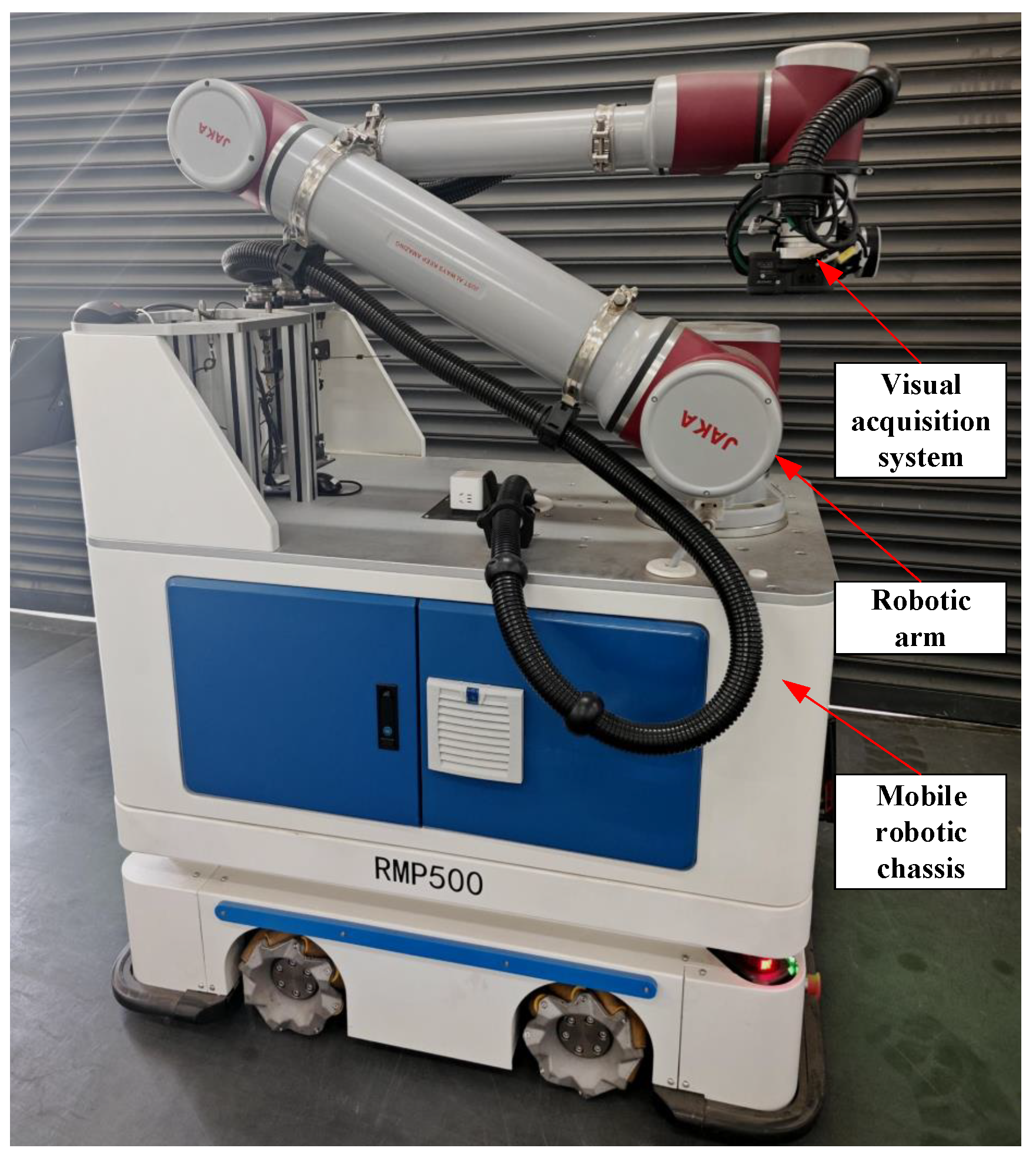
Figure 1 depicts the acquisition system, comprising an MRC-series mobile chassis (KeCong Control Technology Co., Ltd., Zhejiang, China), a JAKA Pro 16 collaborative robot (JAKA Robotics Co., Ltd., Shanghai, China), and an MV-CS200-10GM CMOS camera with an MVL-KF3524M-25MP fixed-focal-length lens and white ring light (HIKROBOT Co., Ltd., Hangzhou, China). The processing platform was a VMC50U five-axis CNC machining center (Kede CNC Co., Ltd., Dalian, China). The inspected tools were square-end, solid WC-Co carbide end mills with internal dataset designations EM-A (AlTiN-coated) and EM-B (AlTiSiN-coated), supplied by Shanghai Aerospace Equipment Manufacturing Co., Ltd. (Shanghai, China) and Changzhou Mingtaishun Cemented Carbide Co., Ltd. (Changzhou, China), respectively. The acquisition-system parameters are listed in

Table 1. Main parameters of tool wear visual acquisition system.

Equipment	Parameter Index
Industrial camera	Resolution: 5472 × 3648; Frame rate: 5.9 fps; Exposure time: 46 μs ∼ 2.5 s
Prime lens	Focal length: 35 mm; F-number: F2.4 ∼ F16; Optical-Distortion: 0.02%
Ring light sources	Color: White LED; Brightness: Adjustable; Lifespan: 30,000 h

; the designations, geometry, machining domains, and cutting-condition ranges are summarized in

Table 2. Designation and main parameters of the inspected end mills.

Code	Coating/Substrate	Diameter (mm)	Flutes	Rake/Clearance (°)	Helix (°)
EM-A	AlTiN/WC-Co	6, 10, 12	2–4	5/5	38
EM-B	AlTiSiN/WC-Co	12, 20	4	8/8	35

and

Table 3. Machining domains and cutting-condition ranges represented in the dataset.

Workpiece	Condition	Tool	${\mathit{v}}_{\mathit{c}}$ (m/min)	${\mathit{f}}_{\mathit{z}}$ (mm/Tooth)	${\mathit{a}}_{\mathit{p}}$ (mm)	${\mathit{a}}_{\mathit{e}}$	Cooling/Lubrication
AISI 1045 steel	180–220 HB	EM-A	80–120	0.03–0.06	0.3–0.8	0.10–0.30 D	Dry/air blast
AISI H13 die steel	48–52 HRC	EM-B	60–100	0.02–0.05	0.2–0.6	0.05–0.20 D	Air blast/MQL

.

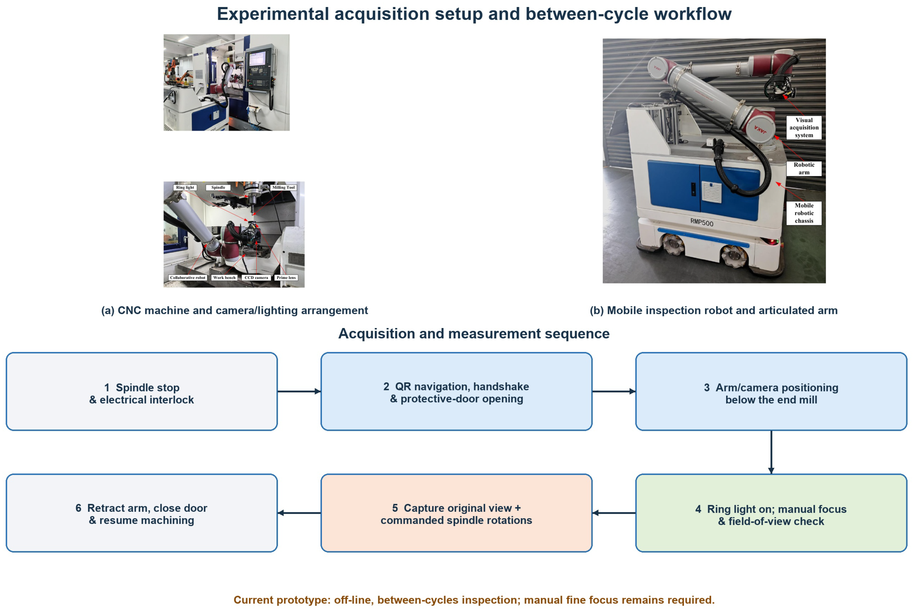
The acquisition sequence is illustrated in Figure 2. After the spindle was stopped and electrically interlocked, the mobile robot navigated to the machine via QR-code localization and established a machine handshake. The protective door was opened, the arm moved the camera beneath the tool, and the ring light was set to a fixed nominal level. Because a fixed lens was used, an operator performed fine focus and verified that the full bottom edge was inside the field of view. One image was then recorded at the original angular position, and additional images were recorded after commanded spindle rotations. The arm was retracted before the machine door was closed. Thus, the present system is an off-line, between-cycles inspection arrangement rather than an in-process or fully autonomous monitor.

The tools were obtained from routine end-milling production rather than a single-factor tool-life experiment. The ranges in Table 3 were reconstructed from production route cards and are reported at the dataset level; exact cumulative cutting time was not retained for every tool. Parameters were selected from supplier recommendations and then reduced, when necessary, to avoid chatter and thermal overload on the VMC50U for the specified tool diameter, workpiece hardness, and radial engagement. This retrospective provenance is considered when interpreting generalization.

2.1.2. Image Acquisition

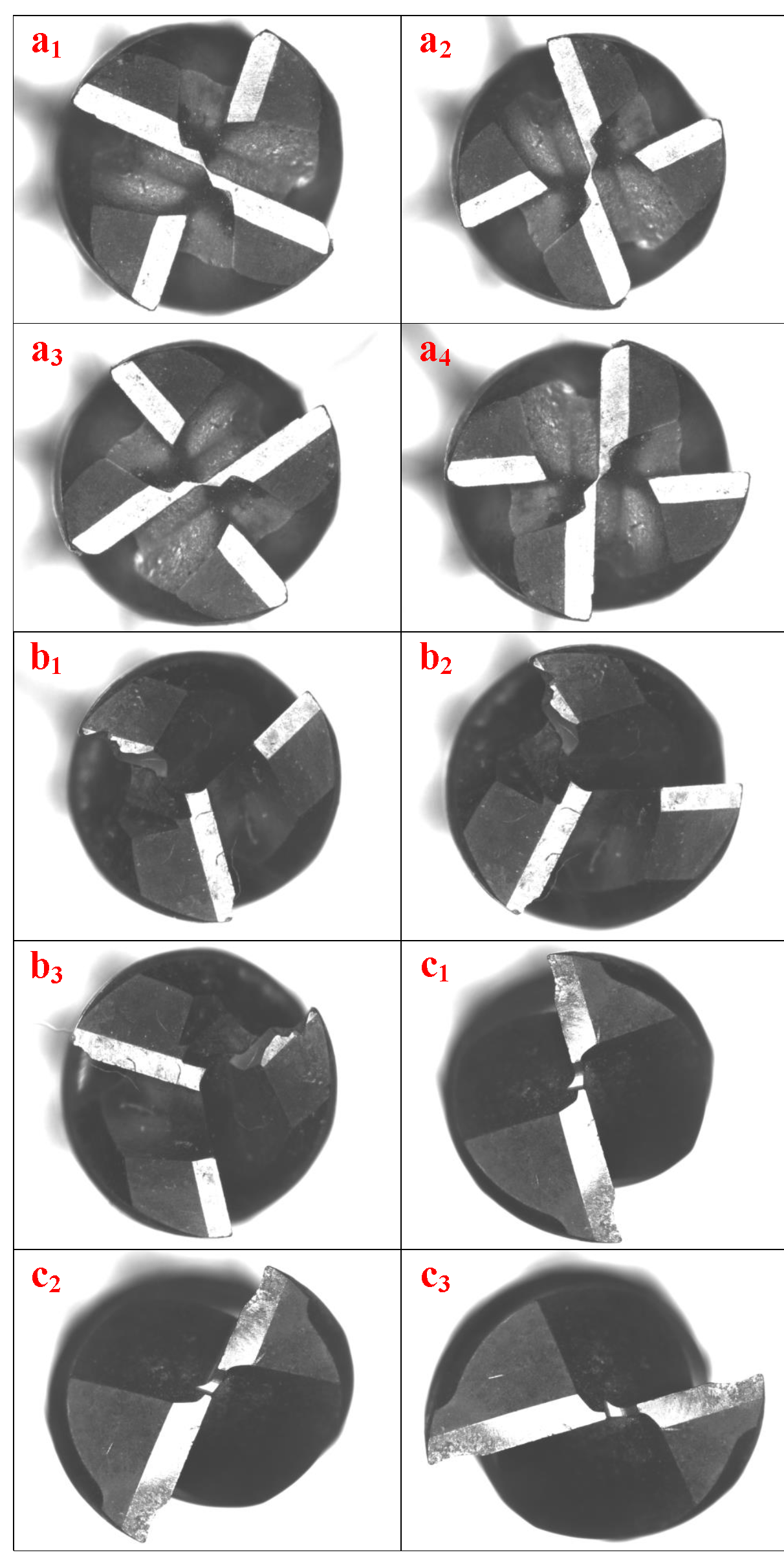
A total of 54 wear carbide end-milling tools with 4 prevalent distinct diameters were selected for bottom-edge image acquisition. The number of blades typically fell within a range of 2 to 4, and the quantity distribution of these tools was as follows (‘n’ denotes the number of tools): size 6 mm (n = 10), size 10 mm (n = 16), size 12 mm (n = 22), size 20 mm (n = 6). To facilitate data collection, four-edged milling tools underwent three random rotations, resulting in four images, including the original. Three-edged and two-edged tools underwent two random rotations, resulting in three images, including the original. As illustrated in Figure 3, image $a_1$ is the raw picture of the four-edged milling tool ($T_1$), while images $a_2$ to $a_4$ depict images obtained by subjecting $T_1$ to random rotations. Image $b_1$ presents the original image of the three-edged milling tool ($T_2$), while image $b_2$ and image $b_3$ denote pictures obtained by rotating $T_2$ at random. Similarly, image $c_1$ showcases the original image of the two-edged milling tool ($T_3$), while image $c_2$ and image $c_3$ mark pictures obtained by stochastic rotations of $T_3$. A total of 234 tool wear images were acquired during the experimental procedure. These images were obtained via physical rotation during acquisition and are treated as raw images in our study; the subsequent augmentation in Section 2.3.1 refers to digital image transformations applied only within the training pipeline.

2.1.3. Data Processing

Determination of Tool Wear Categories

Forms of Tool Failure: Tool failure is the condition in which a cutting tool loses its ability to cut effectively due to wear, breakage, or plastic deformation. There are two main modes of tool failure: tool wear, and tool breakage.

Tool Wear: A natural phenomenon arising from mechanical, chemical, and thermal stresses during machining processes, tool wear manifests as the progressive deterioration of cutting tools due to continuous usage during chip formation. This deterioration leads to increased cutting forces, diminished machining accuracy, and a decline in the quality of the machined surface [13]. Tool wear can be categorized into three primary types based on the location of wear:

• Crater Wear (KT Wear): This type of wear occurs on the rake face, the front surface of the cutting tool that forms the chip. It is characterized by the formation of a crater-like depression on the rake face due to friction and abrasion. Crater wear can lead to impaired chip formation, increased cutting temperature, and accelerated flank wear.
• Flank Wear (VB Wear): This type of wear emerges on the flank face, the rear surface of the cutting tool that contacts the work pieces. It is characterized by a gradual erosion of the tool material, resulting in a reduction in tool strength and an increase in cutting forces. Flank wear is often the most prevalent form of tool wear and a significant factor in determining tool life.
• Notch Wear: This type of wear appears at the intersection of the rake face and flank face, forming a notch or groove along the cutting edge. It is primarily caused by the plastic deformation of the workpiece material and the tool material under high cutting forces. Notch wear can weaken the cutting edge and contribute to premature tool failure.

Flank wear width (VB) is widely used as a quantitative wear indicator. ISO 3685:1993 defines related terminology for single-point turning tools, whereas ISO 8688-2:1989 is the process-relevant standard for end-milling tool-life tests [41,42]. In this study, ISO 3685 is cited only for the general VB terminology; the measurement direction and reference edge follow ISO 8688-2. We do not apply the ISO 3685 turning-tool life threshold and do not infer tool life from the proposed images.

Tool Breakage: Tool breakage in machining operations refers to the sudden and catastrophic failure of a cutting tool, resulting in its sudden fracture or break. Tool breakage encompasses both plastic and brittle fracture mechanisms. This study focuses on the latter, which manifests in various forms, including the following:

• Breakage: Known as catastrophic fracture, this is the most severe form of brittle fracture in cutting tools. It involves catastrophic tool failure characterized by extensive breakage or large fracture surfaces, which can arise from extreme machining conditions, design flaws, or existing cracks.
• Chipping: Known as edge fracture, this is a common type of brittle fracture in cutting tools, primarily caused by excessive impact loads or tool material defects, and typically manifesting as small notches on the cutting edge due to the sudden detachment of small fragments.
• Spalling: This type of brittle fracture in cutting tools, also known as flake fracture, involves the detachment of larger fragments from the tool surface, typically in the form of flakes or scales. Spalling primarily arises from thermal fatigue, chemical wear, and diffusion wear.
• Cracking: Cracking refers to the formation and growth of small cracks in the tool material, which typically originate from fatigue, thermal stress, and impact damage. Cracks can remain dormant or progress until they reach a critical size, leading to sudden chipping, spalling, or breakage.

While tool failure can be catastrophic, ISO 8688-2:1989 and industrial practice distinguish progressive wear from local edge damage [42]. Minor damage does not always prevent continued cutting. To determine representative visible categories, we randomly sampled 100 images and counted five recurrent annotation candidates (

Table 4. Statistics of five primary tool wear types.

Tool Wear Category	Number of Instances	Average Number of Pixels	Total Number of Images
Breakage	434	13.679	100
Chipping	309	3.166
Flank wear	187	2.385
Spalling	11	4.099
Cracking	78	/

).

The class distribution reported in Table 4 is inherently imbalanced, which is a consequence of real wear formation rather than an artifact of dataset construction. In shop-floor milling, most of the visible tool surface remains intact, while wear/damage is typically localized around mechanically and thermally stressed regions—especially along the cutting edge and adjacent flank/rake areas. As a result, “normal/tool-body” pixels dominate spatially, whereas wear-related instances occupy smaller extents and occur with different frequencies. We therefore preserve this natural long-tailed distribution to reflect realistic operating priors and deployment conditions, instead of artificially rebalancing rare phenomena to unrealistic proportions.

The final model taxonomy contains four target classes: breakage, chipping, flank wear, and cracking. Crater and notch wear were discussed as general mechanisms but were not retained because the bottom-edge view did not provide a consistent rake-face/depth-of-cut reference for those labels. Spalling was observed only 11 times and was excluded because it could not support a separate train/validation/test evaluation. Spalling polygons were assigned an ignore index rather than relabeled as another class; an image containing a target class remained usable, while ignored pixels did not contribute to class, mask, or mIoU calculations. This treatment avoids both label conflation and artificial inflation of the common classes.

Data Annotations

Before commencing image annotation, we initially considered employing a combination of physical ground-truth and microscopic measurements to annotate tool wear-land width. However, the laboratory industrial microscope, despite its capacity for high-precision calibration and measurement, exhibited several limitations:

• First, the visual system’s pose could not be self-calibrated and required manual distance adjustments, resulting in poor flexibility, time consumption, and hindering automation.
• Second, the fixed-focus lens limited imaging to a single cutting edge of the tool, severely restricting the extraction of global features and recognition capabilities during model training.
• Third, the system was incapable of annotating tool wear categories, making it incompatible with mainstream annotation software.

Considering these limitations, X-AnyLabeling v2.3.3 was selected because it supports polygon, circle, and point/line annotations in one record [43]. All masks and VB candidate lines were manually reviewed by a second annotator before export.

Ground-Truth Hierarchy and Traceability: Three related but distinct records are used. Class and mask ground truth consists of the adjudicated manual annotations on the robot-acquired images. The regression label used for training and validation is the two-endpoint line obtained from the candidate-line selection rule below and converted to millimeters using the image-specific scale. For the held-out test-set VB MAE, the same physical wear feature is linked by physical-tool ID, flute index, and acquisition view to a microscope reading of that edge; this microscope reading is the operational quantitative reference. The test microscope values are not used for model fitting. Thus, the microscope is a reference instrument for the reported test MAE, not a competing prediction method and not an error-free absolute standard.

Annotation Principles: The model estimates visible damage width; it does not predict tool life. For flank wear, the maximum wear-land width is measured perpendicular to the original cutting edge in accordance with ISO 8688-2:1989 [42]. For chipping or breakage, an analogous local width is recorded perpendicular or parallel to the original edge, as appropriate. Cracking is segmented and classified but is not assigned a VB target when two physically meaningful boundaries cannot be identified.

Annotation Details: In accordance with ISO 8688-2:1989, Clauses 7.5.1 and 7.5.3, flank wear should be measured in a plane parallel to the wear band surface and in a direction perpendicular to the original cutting edge. It is the distance from the original cutting edge to that limit of the wear land that intersects the original flank. The size of chipping should be measured parallel or perpendicular to the original cutting edge on the flank and face, and the location of chipping on the cutting edge should be indicated. Consequently, semantic segmentation is the primary annotation method employed. To facilitate a more comprehensive quantitative assessment of tool wear in this study, we introduced two additional annotation types during image annotation:

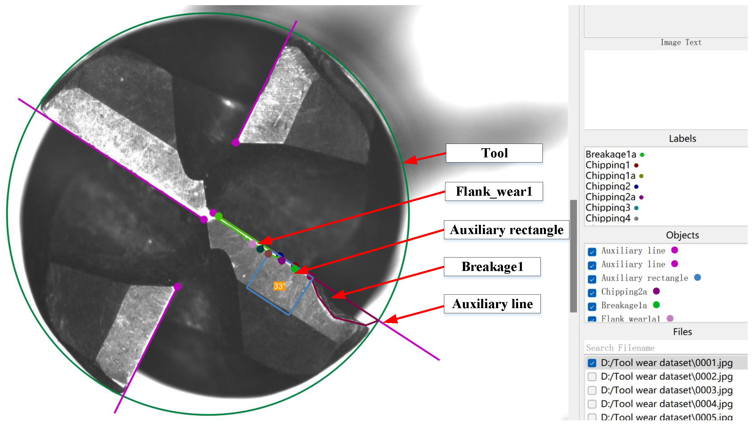
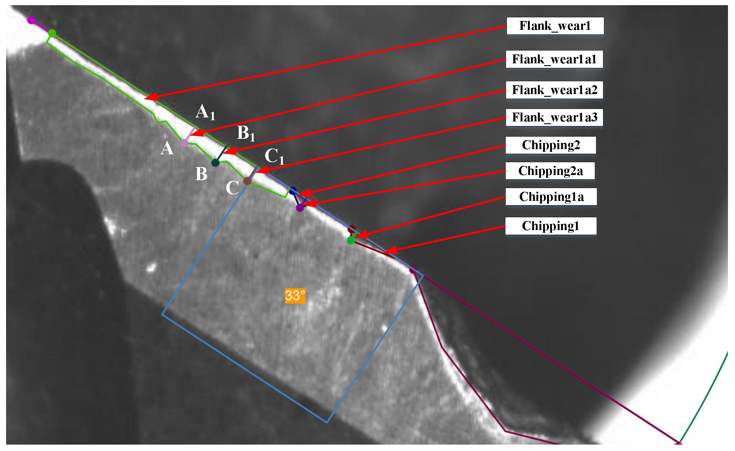
• Tool Bottom-Edge Circumscribed Circle: Represented by ‘Tool’ during annotation, this circle is employed to calculate the scale factor between the actual tool diameter and the pixel diameter. The specific annotations and illustration are marked in Figure 4.
• Wear Band Width VB for the Three Wear Types: The suffix ‘a’ is appended to the annotation type to distinguish between the two wear types. Figure 5 denotes the details of labeling the width of the wear band (VB).

For a regular region, one boundary-to-boundary line is annotated. For an irregular region, the annotator records K candidate endpoint pairs. A preprocessing script calculates the Euclidean length of every candidate, selects the longest pair, and writes only that pair as the two-point regression target. Thus, the annotation interface may contain several candidates, whereas the model consistently outputs two endpoints defining $V{B}_{\max }$. The pixel-space target follows Equation (1) [42]:

$$\begin{array}{cc}\hfill d_k& =\sqrt{{(x_k^{\mathrm{w}}-x_k^{\mathrm{e}})}^2+{(y_k^{\mathrm{w}}-y_k^{\mathrm{e}})}^2},k=1,\dots ,K,\hfill \\ \hfill k^{\ast }& =\arg \underset{k}{\max }{d}_k,V{B}_{\mathrm{pixel}}=d_{k^{\ast }},\hfill \end{array}$$

(1)

where $(x_k^{\mathrm{e}},y_k^{\mathrm{e}})$ and $(x_k^{\mathrm{w}},y_k^{\mathrm{w}})$ are the cutting-edge and outer wear-boundary endpoints of candidate k. The selected pair $k^{\ast }$ supplies the only two points used by the regression head.

The selected pixel distance is converted to a physical dimension using the known tool diameter and its annotated circumscribed-circle diameter according to Equation (2):

$$\begin{array}{c}\hfill D_{\mathrm{real}}=D_{\mathrm{pixel}}\times R,\end{array}$$

(2)

where $D_{\mathrm{real}}$ is the physical width inferred from a robot-acquired image, $D_{\mathrm{pixel}}$ is the measured pixel distance in that image, and $R=D_{\mathrm{tool}}/D_{\mathrm{tool},\mathrm{pixel}}$ is its diameter-based scale in mm/pixel. Two optical systems must be distinguished: The robot-based dataset system uses the MV-CS200-10GM camera, conventional MVL-KF3524M-25MP fixed-focal-length lens, white ring light, fixed nominal pose, and manual fine focusing described in Section 2.1.1; Equation (2) and the diameter ratio apply only to these robot images. The separate microscope reference system uses the G3-GM30M5105 camera and DTCM210-36-M42-AL telecentric lens described in Section 2.3.4, together with its calibrated distance tool, to provide the linked test-set VB reference readings. The telecentric-lens distortion specification therefore characterizes the microscope reference system and is not assigned to the robot camera. For the robot images, the per-image diameter ratio partly compensates for working-distance variation only when the tool end face remains approximately normal to the optical axis. A full robot-camera intrinsic/extrinsic calibration, pose-sensitivity experiment, and repeated-operator gauge repeatability and reproducibility study were not archived. Consequently, 0.010214 mm is an empirical test-set MAE against the separate microscope references under the stated fixed setup, not a claimed camera resolution, metrological uncertainty, or general 0.01 mm accuracy guarantee. This use of ISO 8688-2 concerns the measurement direction and definition of the wear boundary; it is not an ISO-conforming controlled tool-life test, because the tools were collected retrospectively from production.

2.2. Proposed Method

2.2.1. Overview

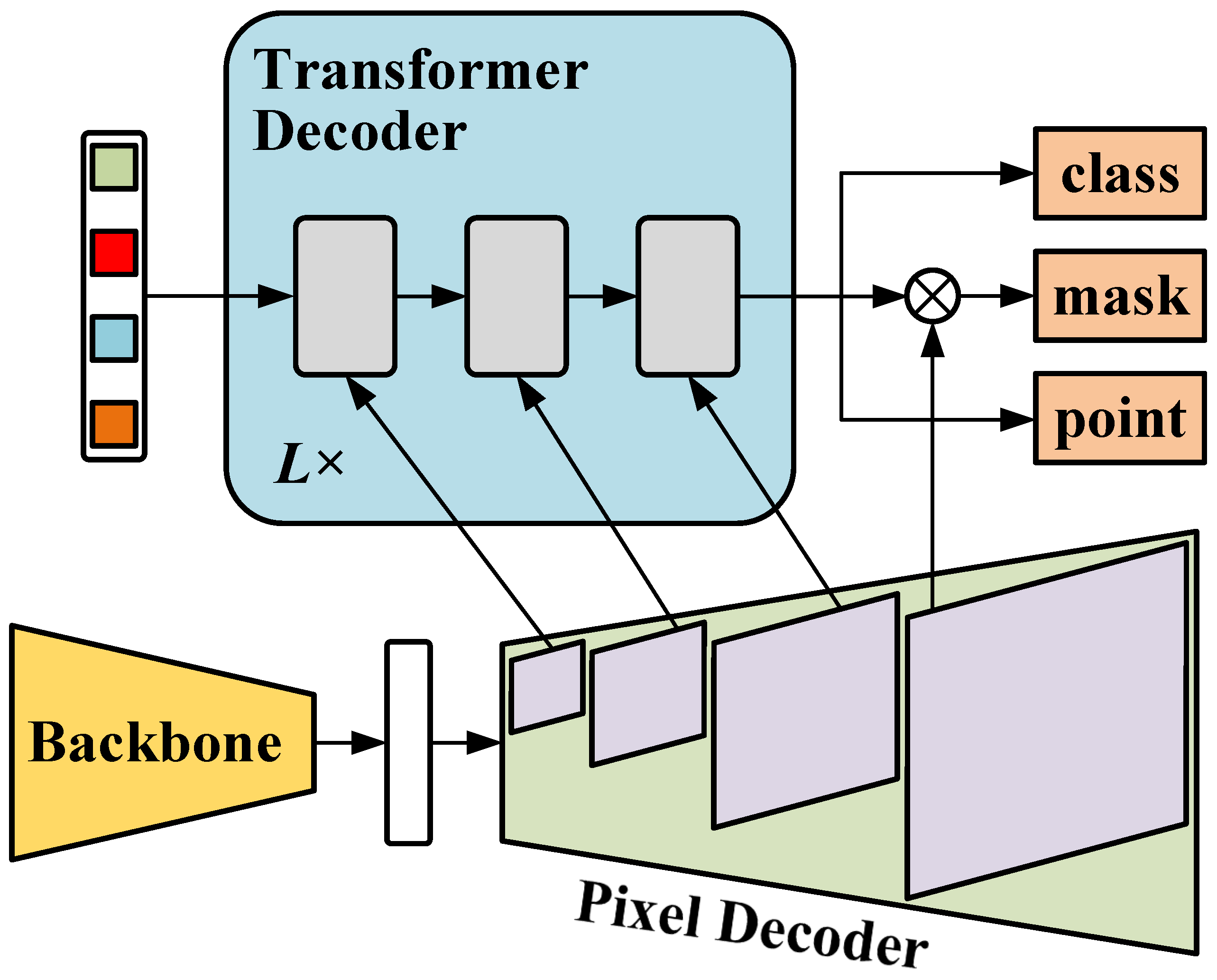
MaskLenNet treats each visible wear or damage region as a query-matched instance and jointly predicts its category, foreground mask, and $V{B}_{\max }$ line. As summarized in Figure 6, four hierarchical backbone features are projected to a common channel dimension, fused by the pixel decoder, and consumed by a nine-layer query decoder. The output for each of 100 queries comprises five class logits (four target classes plus ‘no object’), a binary mask embedding, and four normalized coordinates representing the two endpoints of the selected $V{B}_{\max }$ line. Exact implementation dimensions are listed in

Table 5. Reproducible configuration of MaskLenNet.

Component	Configuration
Input	RGB, $1024\times 1024$
Backbone	Swin-S; patch 4; depths [2, 2, 18, 2]; heads [3, 6, 12, 24]
Backbone outputs	strides [4, 8, 16, 32]; channels [96, 192, 384, 768]
Pixel decoder	4 scales projected to 256 channels
Query decoder	100 queries; 9 layers; 8 attention heads; hidden dimension 256
Wear attention	fused strides 4/8; depthwise kernels 3/5; sigmoid gate; train ROI from annotation; inference ROI from pre-forward circle fit; 8-pixel dilation; pre-cross-attention addition
Outputs/query	5 class logits; mask embedding; 4 normalized endpoint coordinates
Loss balancing	4 learnable log variances $s_t$; initialized to 0
Initialization	ImageNet-1K pretrained Swin-S; new heads initialized with Xavier uniform

.

2.2.2. Backbone

We use the Swin-S variant [44] because the task contains small edge-local defects at high input resolution and benefits from hierarchical features. The implementation uses a $4\times 4$ patch embedding, stage depths [2, 2, 18, 2], attention heads [3, 6, 12, 24], and feature dimensions [96, 192, 384, 768]. The four stage outputs are extracted at strides [4, 8, 16, 32] and projected to 256 channels. Swin and its shifted-window attention are adopted without architectural novelty; our changes are downstream and are described below.

2.2.3. Positional Embedding

To incorporate spatial information, the module uses a sine positional encoding mechanism. Positional encodings are added to each projected feature map, allowing the model to capture the relative positions of objects within the image. This is crucial for maintaining spatial consistency across the various scales processed by the network.

2.2.4. Transformer Decoder

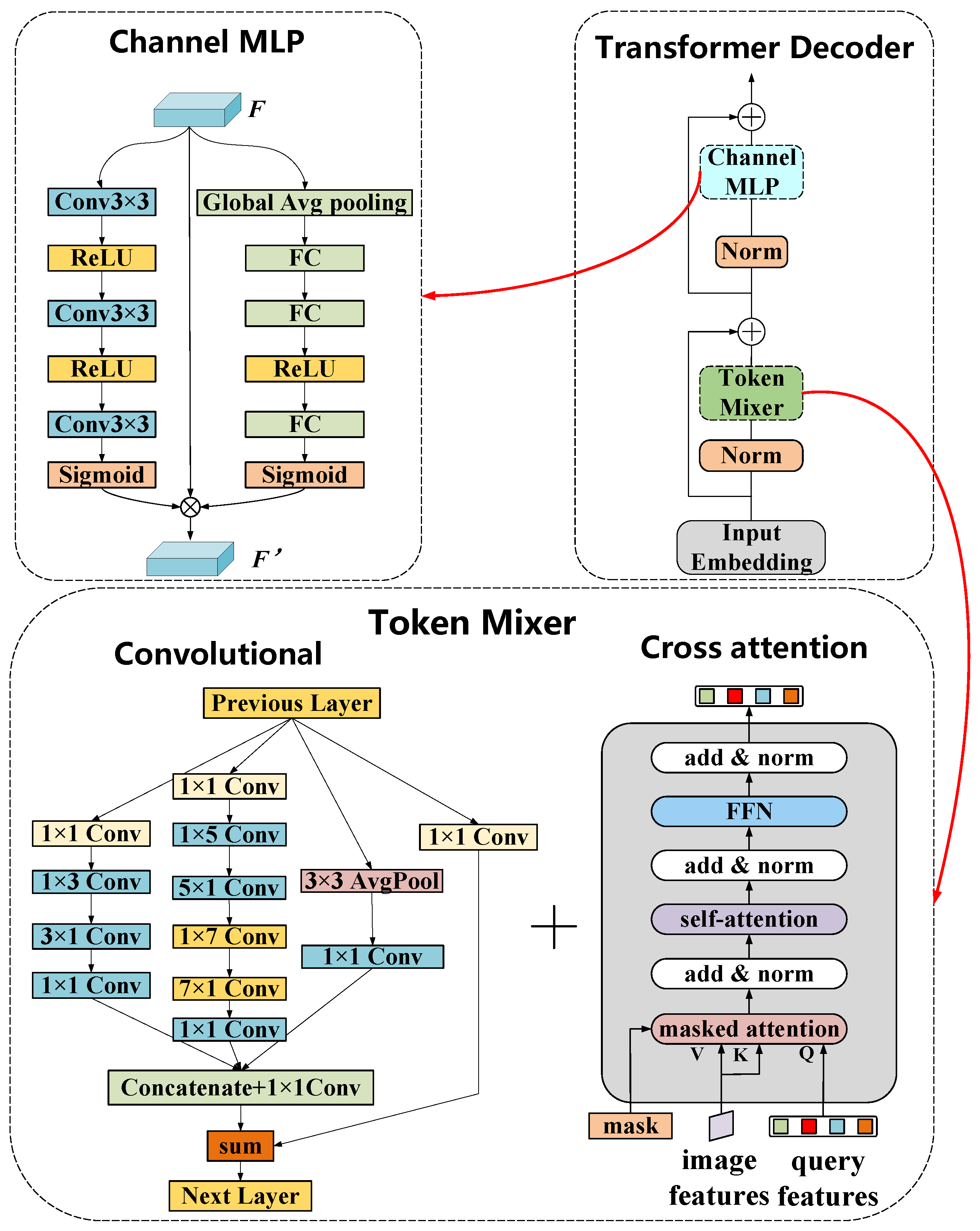
The decoder follows the query-based masked-attention paradigm of Mask2Former [45]. Each of the nine layers contains cross-attention to one feature scale, query self-attention, and a feed-forward block; feature scales are used cyclically from coarse to fine. Patch mixing and channel mixing are adapted from the general MetaFormer concept [46], rather than being claimed as new components.

Patch and Channel–Spatial Mixing: The patch mixer uses parallel depthwise convolutions with $3\times 3$, $5\times 5$, and $7\times 7$ kernels followed by a $1\times 1$ projection, GELU, and a residual connection. The channel gate is generated by global average pooling and a two-layer MLP with reduction ratio 16. The spatial gate is generated by concatenating channel-average and channel-maximum maps and applying a $7\times 7$ convolution. Sigmoid channel and spatial weights modulate the 256-channel feature map before residual addition.

Wear-Attention Branch: Shallow $1/4$- and $1/8$-scale features are fused by parallel $3\times 3$ and $5\times 5$ depthwise convolutions. The gate is conditioned on a binary tool ROI that is available before query decoding; it is not derived from the final wear masks. During training, the ROI is rasterized from the annotated “Tool” circumscribed circle. During inference, the same image-level geometric preprocessing used to estimate $D_{\mathrm{tool},\mathrm{pixel}}$ fits the visible circular tool boundary from the input edge map, rasterizes the fitted disk, and dilates it by eight input pixels to avoid suppressing boundary wear. A circle fit is accepted when its mean absolute radial residual is no greater than five input pixels and detected boundary support covers at least 50% of the circumference. The fitted disk is resized to each feature scale and multiplied with the sigmoid attention map. If either acceptance condition fails, a conservative centered disk using the detected tool diameter is used; no ground-truth ROI, final wear-mask prediction, or microscope information enters inference. The gated edge-local feature is added to the pixel-decoder feature before cross-attention. This wear-oriented ROI gate, the two-point VB target/head, and their joint optimization are the task-specific contributions. Swin, Hungarian query matching, masked attention, and generic channel/spatial mixing are adopted or adapted from prior work.

Figure 7 shows the exact connections among scale projection, feature mixing, masked cross-attention, query self-attention, and the prediction heads. Tensor dimensions, query count, feature scales, and layer count are provided in Table 5 so that the architecture can be reproduced without inferring settings from the schematic.

2.2.5. Prediction Heads

MaskLenNet simultaneously predicts class labels, instance masks, and the two endpoints of the selected $V{B}_{\max }$ line. Outputs are produced per query after Hungarian assignment.

Classification Head: A linear layer maps each query to breakage, chipping, flank wear, cracking, or ‘no object’. The no-object category absorbs unused queries during training and inference.

Regression Head: A three-layer MLP followed by a sigmoid predicts $(x^e,y^e,x^w,y^w)$ in normalized image coordinates. The target is the single longest candidate pair selected by Equation (1); swapped endpoint order is treated as equivalent in the point loss. The pixel length is converted to millimeters with the image-specific scale in Equation (2). For cracking instances without a meaningful width line, point and length losses are masked out.

Segmentation Head: A linear projection converts each query into a 256-dimensional mask embedding; its dot product with the $1/4$-scale pixel embedding yields the binary instance mask.

The proposed novelty therefore lies in the wear-oriented ROI gate, the candidate-to-$V{B}_{\max }$ target transformation, the two-point VB head, and their joint optimization with classification and mask prediction. The backbone and query-based mask machinery are established components used as the comparison foundation.

2.2.6. Loss Function

The training objective uses the bipartite Hungarian assignment introduced for DETR-style set prediction [33]. The matching cost combines class probability, mask overlap, and point distance; Equation (3) denotes the resulting assignment:

$$\begin{array}{c}\hfill \sigma ,\gamma =\mathrm{Hungarian}\left(\mathrm{gt},\mathrm{pred}\right),\end{array}$$

(3)

where $\sigma$ and $\gamma$ represent the index on each matched sample, respectively.

After matching the predictions, the total loss function consists of four loss components (classification loss, mask loss, point loss and length loss) to align the predictions with the ground truth. Below is a detailed breakdown of each component:

Classification Loss (${\mathcal{L}}_{\mathrm{cls}}$): Cross-entropy is applied to the four wear classes and the no-object class following query-based segmentation practice [45]; the matched-instance term is summarized by Equation (4):

$$\begin{array}{c}\hfill \begin{array}{c}\hfill {\mathcal{L}}_{\mathrm{cls}}=-{\displaystyle \frac{1}{N}}{\displaystyle \sum _{i=1}^N}\sum _{c\in \mathcal{C}}{y}_{i,c}log{\widehat{p}}_{i,c},\end{array}\end{array}$$

(4)

where N is the number of assigned queries, $\mathcal{C}$ includes the four target classes and no-object class, $y_{i,c}$ is the one-hot target, and ${\widehat{p}}_{i,c}$ is the predicted probability.

Mask Loss (${\mathcal{L}}_{\mathrm{mask}}$): Binary cross-entropy evaluates the predicted foreground mask against its matched ground-truth mask [45], as shown in Equation (5):

$$\begin{array}{c}\hfill \begin{array}{c}\hfill {\mathcal{L}}_{\mathrm{mask}}=-{\displaystyle \frac{1}{NP}}{\displaystyle \sum _{i=1}^N}{\displaystyle \sum _{u=1}^P}\left[y_{i,u}log{\widehat{m}}_{i,u}+(1-y_{i,u})log(1-{\widehat{m}}_{i,u})\right],\end{array}\end{array}$$

(5)

where P is the number of evaluated pixels, and $y_{i,u}$ and ${\widehat{m}}_{i,u}$ are the ground-truth and predicted mask values at pixel u.

Point Loss (${\mathcal{L}}_{\mathrm{point}}$) Smooth $L_1$ loss [47] measures endpoint error and is evaluated in both endpoint orders, with the lower value retained, as summarized in Equation (6):

$$\begin{array}{c}\hfill \begin{array}{c}\hfill {\mathcal{L}}_{\mathrm{point}}={\displaystyle \frac{1}{N}}{\displaystyle \sum _{i=1}^N}min\left[\mathrm{SmoothL1}({\mathbf{q}}_i,{\widehat{\mathbf{q}}}_i),\mathrm{SmoothL1}(swap\left({\mathbf{q}}_i\right),{\widehat{\mathbf{q}}}_i)\right],\end{array}\end{array}$$

(6)

where ${\mathbf{q}}_i$ and ${\widehat{\mathbf{q}}}_i$ contain the two ground-truth and predicted endpoints, and swap reverses the endpoint order.

Length Loss (${\mathcal{L}}_{\mathrm{length}}$): To maintain accurate predictions of object dimensions, length loss penalizes the squared difference between the predicted line lengths and ground-truth lengths. This term is vital for ensuring that the model accurately estimates the size of the objects, which can be attained by Equation (7):

$$\begin{array}{c}\hfill \begin{array}{c}\hfill {\mathcal{L}}_{\mathrm{length}}={\displaystyle \frac{1}{N}}{\displaystyle \sum _{i=1}^N}{({\ell }_i-{\widehat{\ell }}_i)}^2,\end{array}\end{array}$$

(7)

where ${\ell }_i$ and ${\widehat{\ell }}_i$ are the true and predicted lengths of the selected endpoint pair. Instances without a valid width line are masked from both regression losses.

Total Loss (${\mathcal{L}}_{\mathrm{total}}$): Following uncertainty-based multi-task weighting [48], four learnable log-variance terms $s_t$ adapt the relative task weights. Each $s_t$ is initialized to zero and optimized jointly with the network. The total loss is given by Equation (8):

$$\begin{array}{c}\hfill {\mathcal{L}}_{\mathrm{total}}=\sum _{t\in \{\mathrm{cls},\mathrm{mask},\mathrm{point},\mathrm{length}\}}\left[exp(-s_t){\mathcal{L}}_t+s_t\right].\end{array}$$

(8)

In summary, the overall loss function balances these components to ensure accurate classification, precise segmentation, and reliable boundary detection, while the Hungarian matching loss ensures that the assignments between predicted and actual objects are optimal. This multi-faceted approach helps the model perform well even in challenging conditions, such as fine-grained class distinctions and high-resolution images.

2.3. Experimental Setup

The experiments used the EM-A and EM-B end mills designated in Table 2. Their end-milling workpiece domains, cutting-speed/feed/depth ranges, and dry, air-blast, or MQL conditions are listed in Table 3. These variables describe the industrial provenance of the imaged tools; the learning split is performed by physical tool and not by individual image.

2.3.1. Data Augmentation

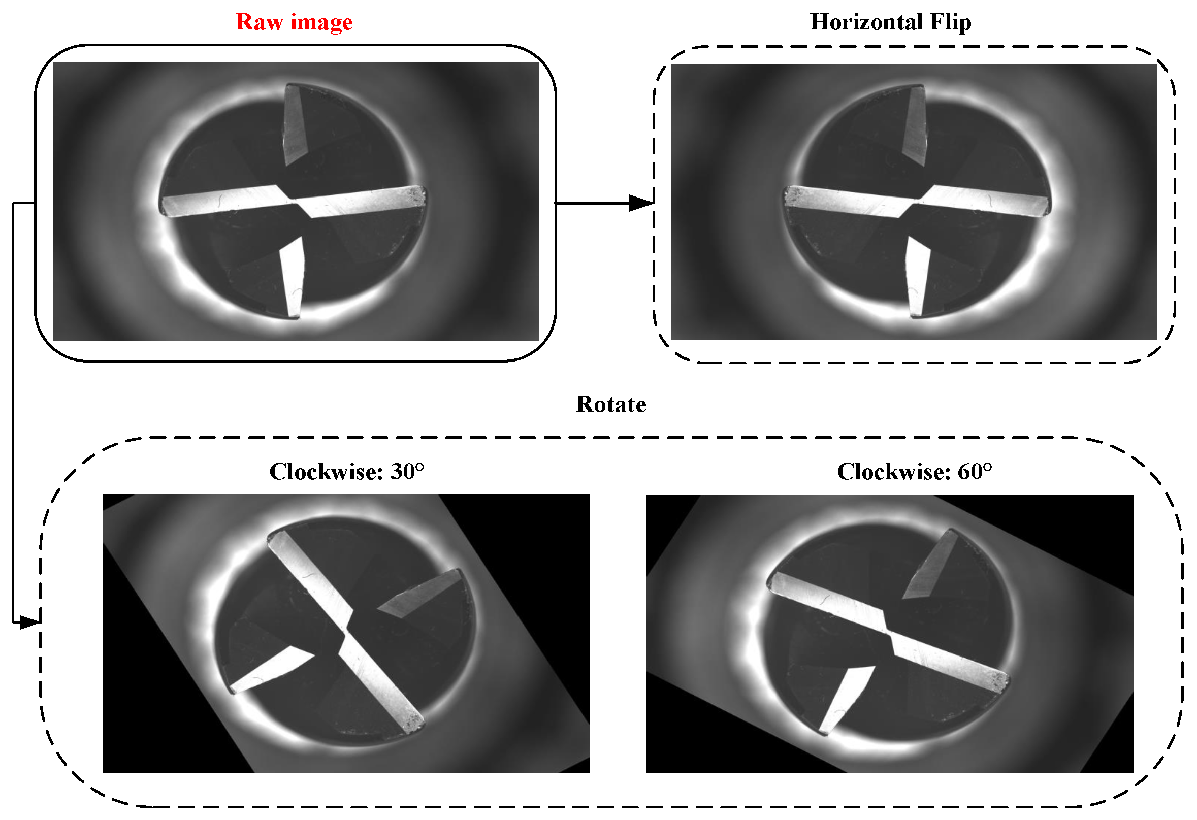
Since the acquired tool images originate from real machining environments and already contain realistic noise, we did not introduce additional synthetic noise during augmentation. Instead, we applied simple geometric transformations, including horizontal flipping and clockwise rotations of 30° and 60° (Figure 8). Starting from 234 raw shop-floor images, applying three non-composed transformations (horizontal flip, 30° rotation, 60° rotation) to each raw image would yield an augmented pool of 936 images (234 × 4). However, under our tool-disjoint protocol, augmentation is applied only to the training split after splitting: the training set contains 165 raw images, and augmentation generates three additional variants per training image, resulting in 660 training images in total (165 + 3 × 165). The validation and test sets contain raw images only, which keeps the evaluation conservative and prevents leakage across different views of the same physical tool.

To prevent leakage across views of the same physical tool, splitting was performed on the physical-tool identifier before any digital augmentation. A seeded group split (seed 2025) assigned 38 tools to training, 8 to validation, and 8 to testing (

Table 6. Summary of the dataset split protocol.

Split	Tools	Raw Images	Images After Augmentation	Augmentation Applied?
Train	38	165	660	Yes: rotations and horizontal flipping
Validation	8	35	35	No: raw images only
Test	8	34	34	No: raw images only

Note: ‘936’ is the theoretical total if all 234 raw images were augmented. In the experiments, only the training split was augmented (165 → 660), while the validation and test splits remained raw.

). Assignment was stratified as far as the small group count allowed by diameter, coating, and presence of the four target classes. All images generated by physical rotation remained with their parent tool. Horizontal flipping and digital rotations were applied only after the training groups were fixed; the validation and test sets contained raw images only.

2.3.2. Implementation Details

All experiments were performed under 64-bit Ubuntu 20.04 LTS using PyTorch 1.13.1, CUDA 11.7, and MMSegmentation 0.30.0 [49] on an Intel Xeon Gold 6230 processor (Intel Corporation, Santa Clara, CA, USA) with eight NVIDIA RTX 3090 GPUs (24 GB each; NVIDIA Corporation, Santa Clara, CA, USA). The held-out test set was used only for final reporting. The tool-disjoint validation set controlled early stopping and hyperparameter selection.

MaskLenNet Parameter Settings and Overfitting Controls: All models used a fixed $1024\times 1024$ input, ImageNet-pretrained initialization when available, AdamW [50], batch size 16, weight decay ${10}^{-2}$, and a cosine learning-rate decay from ${10}^{-4}$ to ${10}^{-6}$. Training was capped at 10 epochs with validation-loss early stopping (patience 3). Leakage was controlled by the tool-disjoint split and train-only augmentation. To assess random initialization and sampling variability, the complete training was repeated with three seeds;

Table 7. Repeated MaskLenNet training runs on the fixed tool-disjoint split.

Seed	Acc (%)	mIoU (%)	MAE (mm)
2024	96.18	95.43	0.010370
2025	96.52	95.75	0.010214
2026	95.96	95.28	0.010510
Mean ± SD	$96.22\pm 0.28$	$95.49\pm 0.24$	$0.010365\pm 0.000148$

reports the held-out results. Full group cross-validation was not performed because only 54 physical tools were available and each fold would further reduce rare-class support; this remains a limitation rather than evidence of broad generalization.

2.3.3. Evaluation Metrics

We report matched-instance classification accuracy, foreground instance mIoU, and VB mean absolute error. The definitions below are important because these metrics do not represent image-level accuracy or full detection average precision. Class and mask metrics use the adjudicated visual annotations; the test-set VB MAE uses the linked microscope reading of the same physical wear feature as its operational reference.

Matched-Instance Classification Accuracy (Acc): After Hungarian assignment, Top-1 class accuracy is computed over matched foreground instances according to Equation (9):

$$\begin{array}{cc}\hfill \mathrm{Acc}(\%)& ={\displaystyle \frac{1}{N_{\mathrm{m}}}}{\displaystyle \sum _{i=1}^{N_{\mathrm{m}}}}\mathbb{I}\left({\widehat{y}}_i=y_i\right)\times 100\%,\hfill \end{array}$$

(9)

where $N_{\mathrm{m}}$ is the number of Hungarian-matched foreground instances, $y_i$ and ${\widehat{y}}_i$ are the true and predicted wear classes, and $\mathbb{I}$ is the indicator function. The displayed 96.52% is therefore a conditional matched-instance classification accuracy, not image-level accuracy or a detection metric. Queries assigned to no-object, duplicate/unmatched foreground predictions, and unmatched ground-truth instances are excluded from both the numerator and denominator of this conditional Acc; images in which a class is absent add no entry. Because the archived prediction files do not support a reliable reconstruction of confidence-thresholded precision, recall, or average precision, this manuscript does not claim that Acc measures end-to-end detection performance. Unmatched cases are nevertheless assigned zero overlap in the mIoU definition below.

Foreground Instance mIoU: Following common semantic-segmentation overlap reporting [51], IoU is first calculated for each matched foreground instance. Unmatched ground-truth and unmatched foreground predictions receive IoU zero. For each target class, instance IoUs are averaged, and the reported mIoU is the macro-average over the four target classes according to Equation (10):

$$\begin{array}{cc}\hfill {\mathrm{IoU}}_j& ={\displaystyle \frac{|A_j\cap B_j|}{|A_j\cup B_j|}},\mathrm{mIoU}={\displaystyle \frac{1}{\left|\mathcal{C}\right|}}\sum _{c\in \mathcal{C}}{\displaystyle \frac{1}{N_{\mathrm{c}}}}\sum _{j:y_j=c}{\mathrm{IoU}}_j,\hfill \end{array}$$

(10)

where $A_j$ and $B_j$ are predicted and ground-truth masks; $\mathcal{C}$ contains breakage, chipping, flank wear, and cracking; and $N_{\mathrm{c}}$ is the number of evaluated instances of class c. Tool-body/background pixels and ignored spalling pixels are excluded. A class absent from a particular image is not averaged as a perfect score; all four classes are present in the complete test set.

Mean Absolute Error (MAE): For instances with a valid two-point target, MAE measures absolute VB error in millimeters according to Equation (11):

$$\begin{array}{c}\hfill \mathrm{MAE}={\displaystyle \frac{1}{N_{\mathrm{v}}}}{\displaystyle \sum _{i=1}^{N_{\mathrm{v}}}}\left|p_i-{\widehat{p}}_i\right|,\end{array}$$

(11)

where $N_{\mathrm{v}}$ is the number of matched test instances with a valid width line and linked microscope reading, $p_i$ is the operational microscope reference for the corresponding tool/flute feature, and ${\widehat{p}}_i$ is the model prediction after pixel-to-millimeter conversion. The same linked microscope references are used for every learned method. This descriptive error does not demonstrate metrological equivalence or agreement with microscopy.

2.3.4. Compared Methods

We compare MaskLenNet with Mask R-CNN [32], Mask2Former [45], ViT-Base [52], BEiT-Base [53], and a U-Net plus rule-based measurement pipeline [25]. These entries are not all “backbone replacements.” Mask R-CNN, Mask2Former, and the U-Net pipeline are complete reference architectures adapted to produce the common four classes, masks, and VB output; the identical two-point regression MLP is attached to matched ROI/query features for Mask R-CNN and Mask2Former. ViT-Base and BEiT-Base are encoder substitutions within the common query-decoder and prediction-head scaffold. Results are therefore reported as two comparison levels—full architecture baselines and controlled encoder substitutions—rather than as if all methods differed at one architectural level.

All learning-based methods use the identical tool-disjoint split, $1024\times 1024$ input, train-only augmentation, pretrained initialization, batch size, maximum epochs, AdamW optimizer, and early-stopping rule. For each method, the learning rate was selected from $\{5\times {10}^{-5},{10}^{-4},2\times {10}^{-4}\}$ using only the validation set. No test-set tuning was performed. This common protocol reduces, but cannot eliminate, the possibility that a baseline would benefit from a larger architecture-specific search.

The selected reference architectures span convolutional, Vision Transformer, masked-attention, and two-stage measurement families. Their parameter counts are reported explicitly rather than treated as matched, and the common validation search is limited. The comparison is therefore dataset-specific and should not be interpreted as a universal ranking of the architectures.

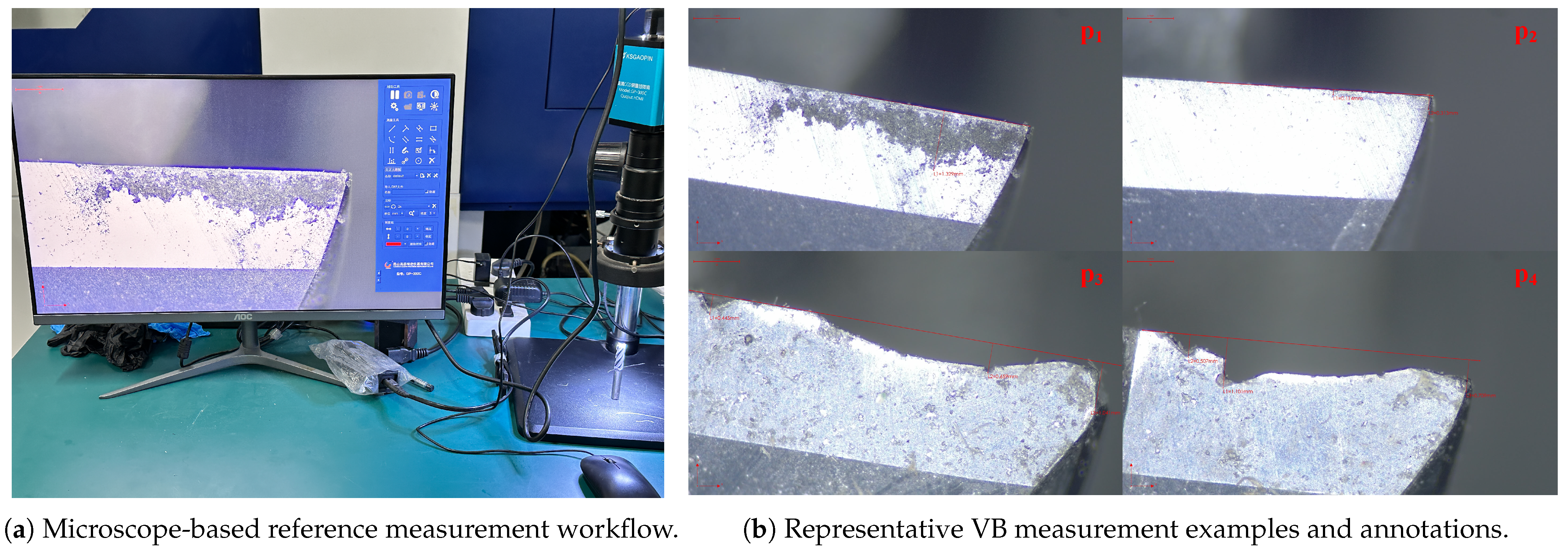
To obtain the operational quantitative reference, we used a G3-GM30M5105 industrial camera and DTCM210-36-M42-AL telecentric lens (LingYun Optics Technology Group Co., Ltd., Beijing, China). The fixed-focus system imaged one cutting edge at a time, and its calibrated distance tool was used to record VB. Each reading was linked to the robot-acquired record by physical-tool ID and flute/feature identity. The instrument parameters are summarized in

Table 8. Parameters of the separate microscope VB reference measurement system.

Equipment	Parameter Index
Industrial camera	Resolution: 5120 × 5120; Frame rate: 20 fps; Optical size: APS-H
Telecentric lens	Magnification: 0.917×; Depth of field: ±0.9 mm; Optical distortion: ≤0.1%
Ring light sources	Color: White LED; Brightness: Adjustable

, and Figure 9 shows the workflow and representative test-set measurements. The displayed example is a 12 mm, four-flute EM-B tool used for end-milling AISI H13 (48–52 HRC) at $v_c=80$ m/min, $f_z=0.04$ mm/tooth, $a_p=0.4$ mm, $a_e=1.2$ mm, with MQL/air blast; the remaining measured tools fall within the ranges of Table 3. The reported MAE values compare each learned method with these linked microscope readings. Because repeated-operator and repeated-microscope measurements were not archived, the readings are operational references, not error-free absolute ground truth.

3. Results

3.1. Main Results

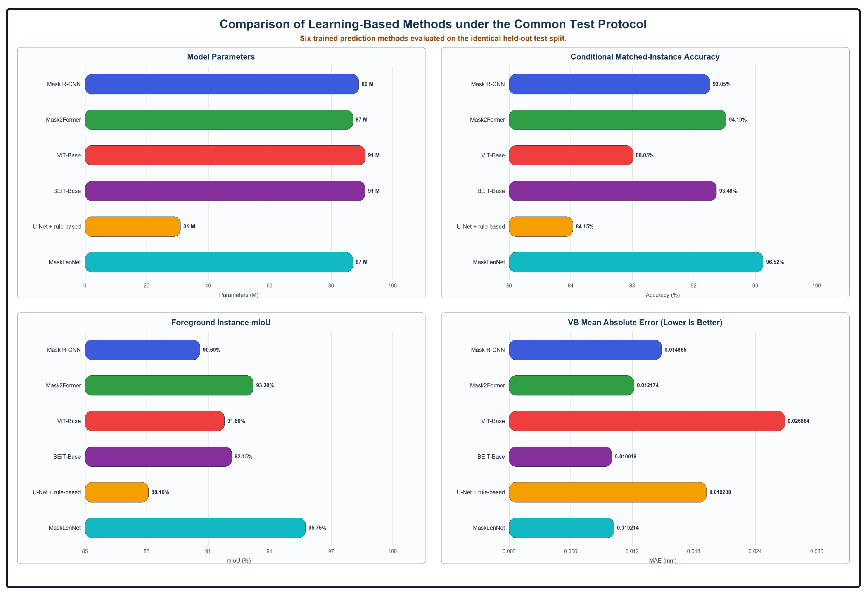
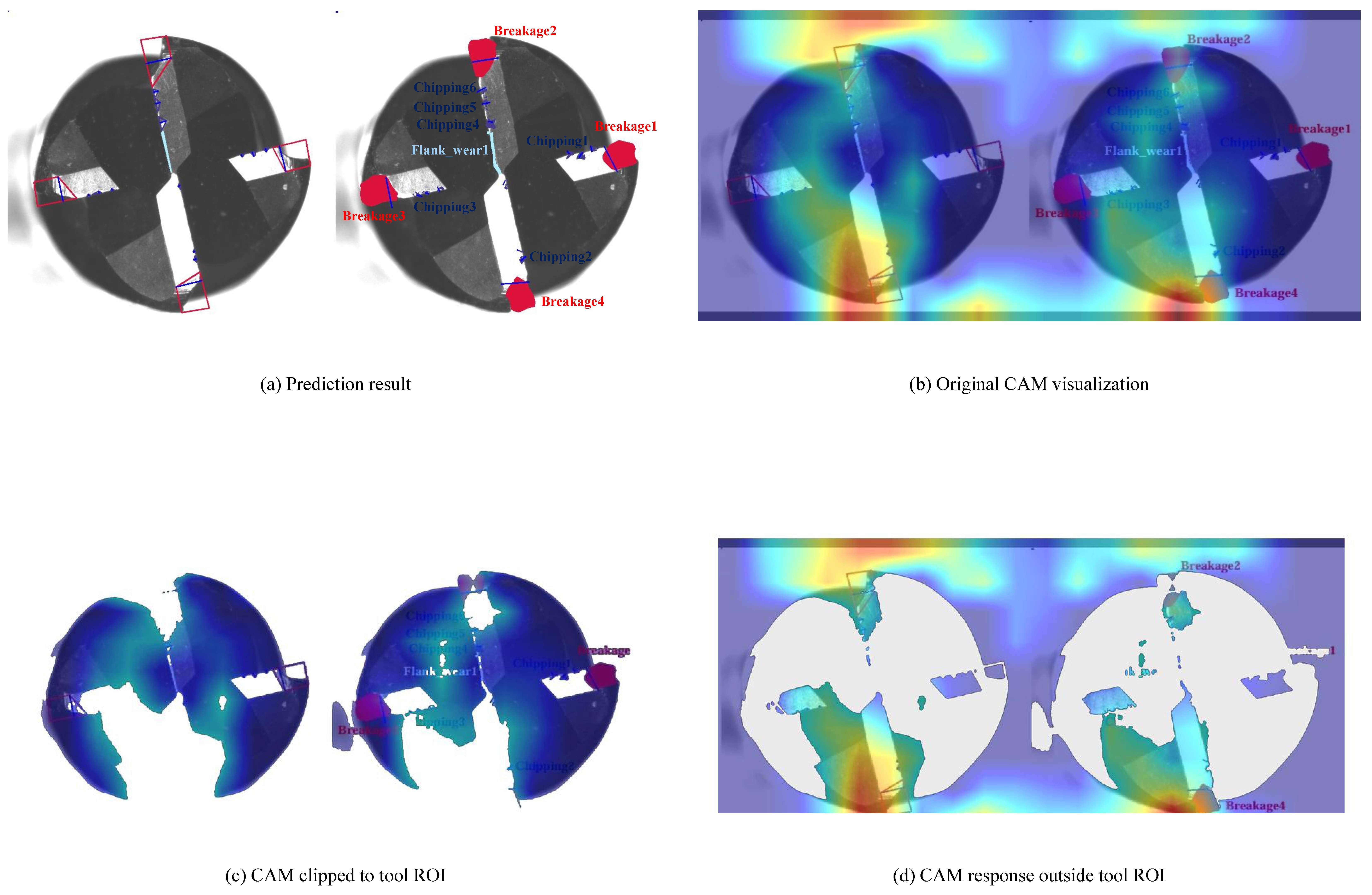
The comparison follows the two levels defined in Section 2.3.4: complete reference architectures adapted to the common outputs, and controlled encoder substitutions within the common query-decoder scaffold. Pretrained initialization and the common training/evaluation protocol are used as specified above. The detailed results are summarized in

Table 9. Main results of the compared learning-based methods on the test set.

Method	#Params	Acc (%)	mIOU (%)	MAE (mm)
Mask R-CNN [32]	89 M	93.05	90.60	0.014865
Mask2Former [45]	87 M	94.10	93.20	0.012174
Visual Transformer (ViT-Base) [52]	91 M	88.05	91.80	0.026884
BEiT-Base [53] (SOTA)	91 M	93.48	92.15	0.010019
Two-stage pipeline
(U-Net + rule-based measure) [25]	31M	84.15	88.10	0.019238
MaskLenNet (Ours)	87 M	96.52	95.75	0.010214

Bold denotes the best value in the corresponding column.

and visualized in Figure 10. The multi-panel Figure 11 combines the prediction visualization and the corresponding Class Activation Map (CAM) [54] views—including a region-of-interest (ROI)-clipped CAM and an outside-ROI response check—to clarify where the network attends when producing wear-related outputs, to verify that dominant activations concentrate on the tool/edge regions rather than the background, and to provide qualitative interpretability support (not causal proof) for the learned discriminative cues. Figure 11a illustrates the prediction result, Figure 11b indicates the original CAM visualization, Figure 11c shows a CAM clipped to the tool ROI (showing the attention distribution only on the physical tool surface), and Figure 11d introduces an outside-ROI response map (explicitly checking whether noticeable attention exists off-tool).

MaskLenNet achieved 96.52% conditional matched-instance accuracy, 95.75% foreground instance mIoU, and 0.010214 mm VB MAE against the linked microscope references. Mask2Former was the strongest segmentation baseline, with 94.10% accuracy and 93.20% mIoU; MaskLenNet therefore improved these metrics by 2.42 and 2.55 percentage points, respectively. BEiT-Base achieved 93.48% accuracy, 92.15% mIoU, and a slightly lower VB MAE of 0.010019 mm. The microscope was used only as the quantitative reference for the learned-method MAE and was not treated as a competing prediction method.

3.2. Computational Performance

Runtime was measured with batch size 1, $1024\times 1024$ input, PyTorch 1.13.1 mixed precision, a single RTX 3090, and 100 warm-up plus 500 timed images. Peak memory included model parameters and inference tensors. These measurements exclude robot navigation, focusing, and image transfer. The results are summarized in

Table 10. Single-GPU computational comparison under the common inference protocol.

Method	Time/Image (ms)	FPS	Peak GPU Memory (GB)
Mask R-CNN	165	6.1	10.2
Mask2Former	134	7.5	9.4
ViT-Base	148	6.8	9.9
BEiT-Base	151	6.6	10.0
U-Net + rule-based measure	74	13.5	5.1
MaskLenNet	141	7.1	9.7

.

3.3. Ablation Study

Within the fixed test split, the proposed query-based instance mask and length-prediction architecture improves the reported classification and mask-overlap metrics over the selected reference methods. Its VB predictions also show a small empirical MAE against the linked microscope references, subject to the uncertainty limitations stated above. To isolate the contribution of the loss design, we varied one loss component at a time while keeping the remaining experimental settings fixed.

For the first ablation study, we replaced the smooth $L_1$ loss in the point loss with the $L_1$ loss. In the second ablation study, we modified the length loss calculation by replacing the squared term with the absolute value.

Table 11. Results of ablation experiments using different loss functions in MaskLenNet.

Point Loss (Smooth ${\mathit{L}}_1$)	Point Loss (${\mathit{L}}_1$)	Length Loss (Squared Term)	Length Loss (Absolute Value)	Acc (%)	mIoU (%)	MAE (mm)
–	✔	✔	–	92.17	90.68	0.010632
✔	–	–	✔	94.69	92.24	0.017836
✔	–	✔	–	96.52	95.75	0.010214

✔ indicates that the loss component is included; – indicates that it is excluded; bold denotes the best joint result in this ablation.

unveils the results of the two ablation experiments.

With $L_1$ point loss and squared length loss, the model obtained 92.17% accuracy, 90.68% mIoU, and 0.010632 mm MAE. With smooth $L_1$ point loss and absolute length loss, it obtained 94.69% accuracy, 92.24% mIoU, and 0.017836 mm MAE. The final smooth $L_1$ plus squared-length configuration produced the best joint result in this ablation (96.52%, 95.75%, and 0.010214 mm).

To clarify component contributions beyond the loss ablation, we progressively enabled wear attention, channel–spatial attention, the multi-task head, and adaptive loss balancing while keeping the data and training pipeline fixed. A0 is the baseline, A1 and A2 add the two attention modules separately, A3 combines them, A4 adds the multi-task head, and A5 adds adaptive loss balancing.

Table 12. Component-wise ablation experiments of MaskLenNet.

ID	Wear Attn	Channel-Spatial Attn	Multi-Task Head	Loss Balancing	Acc (%)	mIoU (%)	MAE (mm)
A0	–	–	–	–	94.30	93.50	0.012857
A1	–	✔	–	–	95.05	94.10	0.011936
A2	✔	–	–	–	95.60	94.80	0.011248
A3	✔	✔	–	–	96.00	95.20	0.010725
A4	✔	✔	✔	–	96.35	95.55	0.010483
A5 (final)	✔	✔	✔	✔	96.52	95.75	0.010214

✔ indicates that the component is enabled; – indicates that it is disabled; bold denotes the final model and its corresponding results.

reports Acc, mIoU, and MAE for this sequence.

4. Discussion

4.1. Interpretation of the Main Results

On the fixed test set, MaskLenNet’s 96.52% accuracy exceeds the two-stage pipeline, Mask R-CNN, ViT-Base, BEiT-Base, and Mask2Former by 12.37, 3.47, 8.47, 3.04, and 2.42 percentage points, respectively. These are absolute percentage-point differences, not relative percentages. Within this dataset, the result is consistent with improved discrimination of the four retained wear classes.

MaskLenNet’s 95.75% mIoU exceeds Mask2Former’s 93.20% by 2.55 percentage points. Because the metric excludes tool-body/background pixels and macro-averages foreground instances, this value should be interpreted specifically as overlap quality for the four annotated wear classes, not as whole-image semantic accuracy.

The VB MAE of MaskLenNet is 1.95% higher than BEiT-Base. All learned-method MAEs use the linked microscope readings as their operational reference. Accordingly, the principal advantage in this experiment is the joint class-mask-VB output and its segmentation performance, not a statistically established equivalence to microscopy.

These findings support promising within-dataset performance. They do not by themselves establish external generalization, robustness to untested acquisition changes, or measurement interchangeability with a microscope.

4.2. Interpretation of the Ablation Results

In the fixed ablation runs, smooth $L_1$ rather than $L_1$ increased accuracy and mIoU by 4.35 and 5.07 percentage points and reduced MAE by 3.93% in relative terms. Using squared rather than absolute length error increased accuracy and mIoU by 1.83 and 3.51 percentage points and reduced MAE by 42.73% in relative terms. Percentage points are used for Acc/mIoU; percentages are reserved for relative MAE changes.

The smooth $L_1$ configuration performed better in these runs and is less sensitive to large residuals by construction [47]. However, no convergence-time comparison or external overfitting analysis was conducted, so the results do not establish that it prevents overfitting or reaches an optimum faster.

The squared-error configuration penalizes large length deviations more strongly and produced the lowest MAE in this ablation. This is an empirical observation for the present split, not a general claim that squared error is always preferable.

Relative to A0, adding channel–spatial attention alone (A1) changes Acc/mIoU by +0.75/+0.60 percentage points and reduces MAE by 7.16%. Wear attention alone (A2) changes Acc/mIoU by +1.30/+1.30 percentage points and reduces MAE by 12.51%. With both modules (A3), Acc and mIoU reach 96.00% and 95.20%, while MAE is 16.58% below A0. These within-split increments are consistent with complementary effects but do not prove causality outside the evaluated data.

Adding the multi-task head (A4) changes Acc/mIoU by +0.35/+0.35 percentage points relative to A3. Adaptive loss balancing (A5) yields the best single run (96.52% Acc, 95.75% mIoU, 0.010214 mm MAE), with +0.17/+0.20 percentage points and a 2.57% relative MAE reduction compared with A4. These modest increments support retaining the components, while repeated external validation is still required.

4.3. Failure Modes and Industrial Workflow

Qualitative review of erroneous cases showed three recurring patterns: cracks occupying only a few pixels were sometimes missed, specular highlights on AlTiSiN tools were occasionally segmented as chipping, and defocus or partial occlusion by adhered chips displaced the predicted VB endpoint. Errors were more frequent for 6 mm tools because the same physical defect covered fewer pixels. The current sample size does not support a reliable factorial analysis of coating, flute count, diameter, and defect size, so these observations are descriptive.

The complete inspection workflow requires the spindle to stop, the door to open, the arm to position, manual fine focus, capture, and retraction. Across the recorded runs, door/handshake required 4–6 s, arm positioning 6–10 s, manual focus 8–15 s, image capture 1–2 s, and retraction/closure 6–10 s, for approximately 25–43 s per inspection, excluding robot travel between machines. Network inference (141 ms/image) is not the dominant delay. Accordingly, the prototype is an off-line, between-cycles, robot-assisted system and is not yet an in-process or fully autonomous monitor.

4.4. Limitations

• Small Correlated Dataset: Only 54 physical tools and 234 raw images are available. The tool-disjoint split prevents cross-view leakage, and three seeds quantify some training variability, but augmentation does not create independent experimental variation, and group cross-validation was not performed.
• Metric Scope: Accuracy is conditional on Hungarian-matched foreground instances and excludes unmatched/duplicate cases; it is not image-level accuracy or full detection average precision. The mIoU definition assigns zero to unmatched cases. Because confidence-thresholded detection outputs were not archived, precision, recall, and average precision could not be reconstructed.
• Measurement Uncertainty: Paired replicate microscope readings, full camera calibration, pose-sensitivity data, confidence intervals, regression agreement, and Bland–Altman limits were not available. Therefore, this study reports MAE against an operational microscope reference only and makes no claim of 0.01 mm metrological accuracy or equivalence to microscopy.
• Acquisition Dependence: Illumination, distance, focus, coolant contamination, chip presence, and pose were not varied systematically. The model depends on the stated camera, lens, ring light, and manual-focus procedure.
• Limited Domain Coverage: No external-site validation was performed with unseen machines or optical systems. Tools were limited to two coating families, four diameters, two workpiece-material domains, and the cutting ranges in Table 3. Spalling was excluded because only 11 instances were available.
• Operational Maturity: Manual focus and machine stoppage remain necessary. Broader tool families, automated focus/calibration, contamination handling, and cross-site evaluation are required before production deployment.

5. Conclusions

This study makes four principal contributions: First, it provides a traceable mobile-robot imaging and annotation workflow for 234 images from 54 coated solid-carbide end mills, together with a physical-tool-disjoint evaluation protocol that prevents rotational views of one tool from crossing data splits. Second, it formulates wear analysis as joint query-based class, instance-mask, and quantitative VB prediction. Third, it introduces a wear-oriented ROI gate and a candidate-line preprocessing rule that converts multiple irregular-region annotations into one two-endpoint $V{B}_{\max }$ target. Fourth, under the stated test protocol, MaskLenNet obtains 96.52% conditional matched-instance accuracy, 95.75% foreground instance mIoU, and 0.010214 mm VB MAE against the operational microscope reference. Relative to Mask2Former, the accuracy and mIoU gains are 2.42 and 2.55 percentage points, respectively.

These results are promising only within the evaluated acquisition system. The study is limited by 54 physical tools, no group cross-validation or external-site test, no systematic illumination/pose/contamination experiment, manual focusing, and the absence of replicate microscope data needed for confidence intervals or agreement analysis. The results therefore do not establish strong cross-domain generalization or equivalence to microscopy. Future work will prioritize a larger multi-site tool-disjoint benchmark, automated optical calibration/focus, rare-class collection, and repeated-measurement uncertainty analysis.

References

1. Hu, L.; Li, W.; Li, B.; Cui, B.; Wang, Z.; Wang, Y. Wear Characteristics and Mechanism Evaluation of High-speed Petal Magnetic Rotor Series Bearings (HPMRSBs) in Vacuum. Compos. Part B Eng. 2026, 313, 113369. [Google Scholar] [CrossRef] [Scilit]
2. Yu, G.; Liu, J.; Hu, L.; Jiang, A.; Wang, L. Motion System Modeling and Acceleration Analysis of Five-axis Hybrid Machine Tool. Adv. Eng. Inform. 2026, 71, 104368. [Google Scholar] [CrossRef] [Scilit]
3. Zhang, J.; Heinemann, R.; Bakker, O.J. Knot-TPP: A Unified Deep Learning Model for Process Incidence and Tool Wear Monitoring in Stacked Drilling. J. Manuf. Mater. Process. 2025, 9, 160. [Google Scholar] [CrossRef] [Scilit]
4. Yu, G.; Hu, L.; Qu, Y. Fretting Slip Wear Mechanism of AlCrN Coated Cemented Carbide Tool on Titanium Alloy TC4 under Ultimate Continuous Cutting. Int. J. Refract. Met. Hard Mater. 2026, 140, 107859. [Google Scholar] [CrossRef] [Scilit]
5. Hashmi, A.W.; Mali, H.S.; Meena, A.; Khilji, I.A.; Hashmi, M.F. Machine Vision for the Measurement of Machining Parameters: A Review. Mater. Today Proc. 2022, 56, 1939–1946. [Google Scholar] [CrossRef] [Scilit]
6. Pimenov, D.Y.; Bustillo, A.; Wojciechowski, S.; Sharma, V.S.; Gupta, M.K.; Kuntoğlu, M. Artificial Intelligence Systems for Tool Condition Monitoring in Machining: Analysis and Critical Review. J. Intell. Manuf. 2023, 34, 2079–2121. [Google Scholar]
7. Liu, Y.; Guo, L.; Gao, H.; You, Z.; Ye, Y.; Zhang, B. Machine Vision Based Condition Monitoring and Fault Diagnosis of Machine Tools Using Information from Machined Surface Texture: A Review. Mech. Syst. Signal Process. 2022, 164, 108068. [Google Scholar] [CrossRef] [Scilit]
8. Agarwal, A.; Potthoff, N.; Shah, A.M.; Mears, L.; Wiederkehr, P. Analyzing the Evolution of Tool Wear Area in Trochoidal Milling of Inconel 718 Using Image Processing Methodology. Manuf. Lett. 2022, 33, 373–379. [Google Scholar] [CrossRef] [Scilit]
9. Otsu, N. A Threshold Selection Method from Gray-Level Histograms. IEEE Trans. Syst. Man Cybern. 1979, 9, 62–66. [Google Scholar] [CrossRef] [Scilit]
10. Shahabi, H.H.; Ratnam, M.M. On-Line Monitoring of Tool Wear in Turning Operation in the Presence of Tool Misalignment. Int. J. Adv. Manuf. Technol. 2008, 38, 718–727. [Google Scholar]
11. Shahabi, H.H.; Low, T.H.; Ratnam, M.M. Notch Wear Detection in Cutting Tools Using Gradient Approach and Polynomial Fitting. Int. J. Adv. Manuf. Technol. 2008, 40, 1057–1066. [Google Scholar] [CrossRef] [Scilit]
12. Shahabi, H.H.; Ratnam, M.M. In-Cycle Detection of Built-Up Edge (BUE) from 2-D Images of Cutting Tools Using Machine Vision. Int. J. Adv. Manuf. Technol. 2010, 46, 1179–1189. [Google Scholar]
13. Soori, M.; Arezoo, B. Cutting Tool Wear Prediction in Machining Operations, a Review. J. New Technol. Mater. 2022, 12, 113–128. [Google Scholar]
14. Lachance, S.; Bauer, R.; Warkentin, A. Application of Region Growing Method to Evaluate the Surface Condition of Grinding Wheels. Int. J. Mach. Tools Manuf. 2004, 44, 823–829. [Google Scholar] [CrossRef] [Scilit]
15. García-Ordás, M.T.; Alegre-Gutiérrez, E.; Alaiz-Rodríguez, R.; González-Castro, V. Tool Wear Monitoring Using an Online, Automatic and Low Cost System Based on Local Texture. Mech. Syst. Signal Process. 2018, 112, 98–112. [Google Scholar] [CrossRef] [Scilit]
16. Bagga, P.J.; Makhesana, M.A.; Patel, K.M. A Novel Approach of Combined Edge Detection and Segmentation for Tool Wear Measurement in Machining. Prod. Eng. 2021, 15, 519–533. [Google Scholar] [CrossRef] [Scilit]
17. Barreiro, J.; Castejón, M.; Alegre, E.; Hernández, L.K. Use of Descriptors Based on Moments from Digital Images for Tool Wear Monitoring. Int. J. Mach. Tools Manuf. 2008, 48, 1005–1013. [Google Scholar] [CrossRef] [Scilit]
18. Ye, Z.; Wu, Y.; Ma, G.; Li, H.; Cai, Z.; Wang, Y. Visual High-Precision Detection Method for Tool Damage Based on Visual Feature Migration and Cutting Edge Reconstruction. Int. J. Adv. Manuf. Technol. 2021, 114, 1341–1358. [Google Scholar] [CrossRef] [Scilit]
19. Fernández-Robles, L.; Sánchez-González, L.; Díez-González, J.; Castejón-Limas, M.; Pérez, H. Use of Image Processing to Monitor Tool Wear in Micro Milling. Neurocomputing 2021, 452, 333–340. [Google Scholar] [CrossRef] [Scilit]
20. Domínguez-Monferrer, C.; Fernández-Pérez, J.; De Santos, R.; Miguélez, M.H.; Cantero, J.L. Machine Learning Approach in Non-Intrusive Monitoring of Tool Wear Evolution in Massive CFRP Automatic Drilling Processes in the Aircraft Industry. J. Manuf. Syst. 2022, 65, 622–639. [Google Scholar] [CrossRef] [Scilit]
21. Wang, P.; Liu, Z.; Gao, R.X.; Guo, Y. Heterogeneous Data-Driven Hybrid Machine Learning for Tool Condition Prognosis. CIRP Ann. 2019, 68, 455–458. [Google Scholar] [CrossRef] [Scilit]
22. Bergs, T.; Holst, C.; Gupta, P.; Augspurger, T. Digital Image Processing with Deep Learning for Automated Cutting Tool Wear Detection. Procedia Manuf. 2020, 48, 947–958. [Google Scholar] [CrossRef] [Scilit]
23. Lin, W.-J.; Chen, J.-W.; Jhuang, J.-P.; Tsai, M.-S.; Hung, C.-L.; Li, K.-M.; Young, H.-T. Integrating Object Detection and Image Segmentation for Detecting the Tool Wear Area on Stitched Image. Sci. Rep. 2021, 11, 19938. [Google Scholar] [CrossRef] [Scilit] [PubMed]
24. Wu, C.; Wang, S. Tool Wear Assessment and Life Prediction Model Based on Image Processing and Deep Learning. Int. J. Adv. Manuf. Technol. 2023, 126, 1303–1315. [Google Scholar] [CrossRef] [Scilit]
25. Ronneberger, O.; Fischer, P.; Brox, T. U-Net: Convolutional Networks for Biomedical Image Segmentation. In Medical Image Computing and Computer-Assisted Intervention—MICCAI 2015; Ronneberger, O., Fischer, P., Brox, T., Eds.; Part III; Springer: Cham, Switzerland, 2015; pp. 234–241. [Google Scholar]
26. Li, Y.; Hong, G.S.; Zhu, K. Robust and Fast Monitoring Method of Micro-Milling Tool Wear Using Image Processing. Chin. J. Mech. Eng. 2025, 38, 70. [Google Scholar] [CrossRef] [Scilit]
27. Singh, G.; Agarwal, A.; Desai, K.A.; Mears, L. Implementation of Vision Transformer Model for Robust Tool Wear Monitoring in Milling of Inconel 718. Machines 2026, 14, 589. [Google Scholar] [CrossRef] [Scilit]
28. Liu, Y.; Zou, L.; Wang, W.; He, H.; Song, S. Acoustic-Force Fusion with Stacking Ensemble Learning for Wear Recognition of Pyramid Abrasive Belts under Variable Grinding Conditions. Mech. Syst. Signal Process. 2026, 250, 114120. [Google Scholar] [CrossRef] [Scilit]
29. Schlegel, C.; Molitor, D.A.; Kubik, C.; Martin, D.M.; Groche, P. Tool Wear Segmentation in Blanking Processes with Fully Convolutional Networks Based Digital Image Processing. J. Mater. Process. Technol. 2024, 324, 118270. [Google Scholar] [CrossRef] [Scilit]
30. Li, Z.; Huo, D.; Meurer, M.; Bergs, T. Efficient Cutting Tool Wear Segmentation Based on Segment Anything Model. In International Manufacturing Science and Engineering Conference; American Society of Mechanical Engineers: New York, NY, USA, 2024; Volume 88117, p. V002T07A002. [Google Scholar]
31. Yoo, Y.; Yang, G.; Park, K.; Hyun, Y.; Jeong, S. Extendable Machine Tool Wear Monitoring Process Using Image Segmentation Based Deep Learning Model and Automatic Detection of Depth of Cut Line. Eng. Appl. Artif. Intell. 2024, 135, 108570. [Google Scholar] [CrossRef] [Scilit]
32. He, K.; Gkioxari, G.; Dollár, P.; Girshick, R. Mask R-CNN. In Proceedings of the IEEE International Conference on Computer Vision; IEEE: New York, NY, USA, 2017; pp. 2961–2969. [Google Scholar]
33. Carion, N.; Massa, F.; Synnaeve, G.; Usunier, N.; Kirillov, A.; Zagoruyko, S. End-to-End Object Detection with Transformers. In European Conference on Computer Vision; Springer: Cham, Switzerland, 2020; pp. 213–229. [Google Scholar]
34. García-Ordás, M.T.; Alegre, E.; González-Castro, V.; Alaiz-Rodríguez, R. A Computer Vision Approach to Analyze and Classify Tool Wear Level in Milling Processes Using Shape Descriptors and Machine Learning Techniques. Int. J. Adv. Manuf. Technol. 2017, 90, 1947–1961. [Google Scholar] [CrossRef] [Scilit]
35. Wu, X.; Liu, Y.; Zhou, X.; Mou, A. Automatic Identification of Tool Wear Based on Convolutional Neural Network in Face Milling Process. Sensors 2019, 19, 3817. [Google Scholar] [CrossRef] [Scilit] [PubMed]
36. Lutz, B.; Kisskalt, D.; Regulin, D.; Reisch, R.; Schiffler, A.; Franke, J. Evaluation of Deep Learning for Semantic Image Segmentation in Tool Condition Monitoring. In 2019 18th IEEE International Conference on Machine Learning and Applications (ICMLA); IEEE: New York, NY, USA, 2019; pp. 2008–2013. [Google Scholar]
37. Lutz, B.; Reisch, R.; Kisskalt, D.; Avci, B.; Regulin, D.; Knoll, A.; Franke, J. Benchmark of Automated Machine Learning with State-of-the-Art Image Segmentation Algorithms for Tool Condition Monitoring. Procedia Manuf. 2020, 51, 215–221. [Google Scholar] [CrossRef] [Scilit]
38. Pan, Y.; Xu, G.; Xiong, Z.; Li, F.; Hu, B.; Sun, Y.; Pan, C.; Wang, Y. NJUST-CCTD: An Image Database for Milling Tool Wear Classification with Deep Learning. Int. J. Adv. Manuf. Technol. 2023, 127, 1–18. [Google Scholar] [CrossRef] [Scilit]
39. De Pauw, L.; Jacobs, T.; Goedemé, T. MATWI: A Multimodal Automatic Tool Wear Inspection Dataset and Baseline Algorithms. In International Conference on Computer Vision Systems; Springer: Cham, Switzerland, 2023; pp. 255–269. [Google Scholar]
40. Pan, Y.; Hao, L.; He, J.; Ding, K.; Yu, Q.; Wang, Y. Deep Convolutional Neural Network Based on Self-Distillation for Tool Wear Recognition. Eng. Appl. Artif. Intell. 2024, 132, 107851. [Google Scholar] [CrossRef] [Scilit]
41. ISO 3685:1993; Tool-Life Testing with Single-Point Turning Tools. ISO: Geneva, Switzerland, 1993.
42. ISO 8688-2:1989; Tool Life Testing in Milling–Part 2: End Milling. ISO: Geneva, Switzerland, 1989.
43. Wang, W.; CVHub. X-AnyLabeling: Advanced Auto Labeling Solution with Added Features, version 2.3.3. Available online: https://github.com/CVHub520/X-AnyLabeling (accessed on 2 July 2026).
44. Liu, Z.; Lin, Y.; Cao, Y.; Hu, H.; Wei, Y.; Zhang, Z.; Lin, S.; Guo, B. Swin Transformer: Hierarchical Vision Transformer Using Shifted Windows. In Proceedings of the IEEE/CVF International Conference on Computer Vision; IEEE/CVF: New York, NY, USA, 2021; pp. 10012–10022. [Google Scholar]
45. Cheng, B.; Misra, I.; Schwing, A.G.; Kirillov, A.; Girdhar, R. Masked-Attention Mask Transformer for Universal Image Segmentation. In Proceedings of the IEEE/CVF Conference on Computer Vision and Pattern Recognition; IEEE/CVF: New York, NY, USA, 2022; pp. 1290–1299. [Google Scholar]
46. Yu, W.; Luo, M.; Zhou, P.; Si, C.; Zhou, Y.; Wang, X.; Feng, J.; Yan, S. MetaFormer Is Actually What You Need for Vision. In 2022 IEEE/CVF Conference on Computer Vision and Pattern Recognition (CVPR); IEEE: New York, NY, USA, 2022; pp. 10809–10819. [Google Scholar]
47. Girshick, R. Fast R-CNN. In Proceedings of the IEEE International Conference on Computer Vision; IEEE: New York, NY, USA, 2015; pp. 1440–1448. [Google Scholar]
48. Kendall, A.; Gal, Y.; Cipolla, R. Multi-Task Learning Using Uncertainty to Weigh Losses for Scene Geometry and Semantics. In Proceedings of the IEEE/CVF Conference on Computer Vision and Pattern Recognition; IEEE/CVF: New York, NY, USA, 2018; pp. 7482–7491. [Google Scholar]
49. MMSegmentation Contributors. MMSegmentation: OpenMMLab Semantic Segmentation Toolbox and Benchmark, version 0.30.0. Available online: https://github.com/open-mmlab/mmsegmentation (accessed on 2 July 2026).
50. Loshchilov, I.; Hutter, F. Decoupled Weight Decay Regularization. In Proceedings of the International Conference on Learning Representations, New Orleans, LA, USA, 6–9 May 2019. [Google Scholar]
51. Long, J.; Shelhamer, E.; Darrell, T. Fully Convolutional Networks for Semantic Segmentation. In Proceedings of the IEEE Conference on Computer Vision and Pattern Recognition; IEEE: New York, NY, USA, 2015; pp. 3431–3440. [Google Scholar]
52. Dosovitskiy, A.; Beyer, L.; Kolesnikov, A.; Weissenborn, D.; Zhai, X.; Unterthiner, T.; Dehghani, M.; Minderer, M.; Heigold, G.; Gelly, S. An Image is Worth 16x16 Words: Transformers for Image Recognition at Scale. In Proceedings of the International Conference on Learning Representations, Virtual, 3–7 May 2021. [Google Scholar]
53. Bao, H.; Dong, L.; Wei, F. BEiT: BERT Pre-Training of Image Transformers. In Proceedings of the International Conference on Learning Representations, Virtual, 25–29 April 2022. [Google Scholar]
54. Zhou, B.; Khosla, A.; Lapedriza, A.; Oliva, A.; Torralba, A. Learning Deep Features for Discriminative Localization. In Proceedings of the IEEE Conference on Computer Vision and Pattern Recognition; IEEE: New York, NY, USA, 2016; pp. 2921–2929. [Google Scholar]
Figure 1. The proposed tool visual acquisition system based on the mobile inspection robot.
Jmmp 10 00286 g001
Figure 2. Experimental acquisition sequence: (1) spindle stop and safety interlock, (2) robot-to-machine handshake and door opening, (3) arm positioning below the end mill, (4) ring-light activation and manual fine focus, (5) bottom-edge image capture at the original and rotated angular positions, and (6) arm retraction and door closure.
Jmmp 10 00286 g002
Figure 3. Tool images acquired by the visual acquisition system: (a1a4) original and three rotated views of a four-flute tool; (b1b3) original and two rotated views of a three-flute tool; and (c1c3) original and two rotated views of a two-flute tool.
Jmmp 10 00286 g003
Figure 4. Annotations of tool wear and breakage categories. In this annotation scheme, ‘Tool’ represents the circumscribed circle of the tool’s bottom edge, and a numerical suffix following the wear type distinguishes the number of instances of the wear type. For instance, ‘Flank_wear1’ denotes the first flank wear region in the given image. Additionally, an auxiliary line is superimposed on each cutting edge to facilitate the annotation of wear regions. An auxiliary rectangle is employed to ensure that the line representing the wear-band width is perpendicular to the cutting edge, thereby minimizing manual annotation errors. The cropped annotation-software panel is shown only to illustrate the labeling workflow and is not an analytical result.
Jmmp 10 00286 g004
Figure 5. Candidate-line annotation and conversion to the two-point V B max target. A regular region uses one endpoint pair. For an irregular region such as ‘Flank_wear1’, three candidate lines (A A 1 , B B 1 , and C C 1 ) are recorded perpendicular to the original cutting edge. Their pixel lengths are calculated automatically, and only the endpoints of the longest candidate are exported as the model’s two-point target.
Jmmp 10 00286 g005
Figure 6. MaskLenNet architecture and tensor flow. A 3 × 1024 × 1024 image produces Swin stage features at 1 / 4 , 1 / 8 , 1 / 16 , and 1 / 32 resolution with 96, 192, 384, and 768 channels. The pixel decoder projects all scales to 256 channels. A nine-layer, eight-head decoder updates 100 queries and feeds class, mask, and two-point VB heads. Colors distinguish feature maps, processing modules, attention operations, and output heads; they are schematic and do not encode numerical values.
Jmmp 10 00286 g006
Figure 7. Detailed decoder connections. Four 256-channel pixel-decoder scales feed a nine-layer decoder in cyclic order. Each layer applies masked cross-attention, eight-head self-attention, and a feed-forward block to 100 queries. Channel–spatial mixing modulates the scale feature, while the wear-attention branch injects ROI-constrained edge-local features before cross-attention. Block colors distinguish convolutional, normalization, activation, attention, and feature/output elements; red arrows indicate the feature-injection path, and colors do not represent measured magnitudes.
Jmmp 10 00286 g007
Figure 8. The process of the image augmentation. For each raw image, three additional variations are generated. These variations are created by applying a horizontal flip and clockwise rotations of 30 and 60 to the original image (i.e., two rotated variants generated independently from the original).
Jmmp 10 00286 g008
Figure 9. Microscope-based VB reference workflow and examples. Panel (a) shows the camera, telecentric lens, calibration, and single-edge measurement; the Chinese interface text identifies acquisition and measurement-tool menus only, and the red scale bar represents 1 mm. Panel (b) shows four representative cutting-edge measurement views (p1p4) for the 12 mm EM-B/H13 condition stated in the text; red lines and labels indicate the measured wear widths. The microscope readings are used as quantitative references; no equivalence claim is made because agreement intervals and repeated-operator uncertainty were unavailable.
Jmmp 10 00286 g009
Figure 10. Statistical comparison of the six learning-based methods on the held-out test set. All displayed MAE values are calculated against the same linked microscope reference readings; the reference instrument is not a plotted method.
Jmmp 10 00286 g010
Figure 11. Multi-panel CAM-based interpretability analysis with tool-ROI leakage check: (a) prediction result; (b) original CAM; (c) CAM clipped to the tool ROI; and (d) CAM response outside the tool ROI. In panel (a), red masks/labels denote predicted breakage, blue masks/labels denote predicted chipping or flank wear, and cyan lines denote predicted width segments. In the CAM panels, colors progress from blue (low activation) through green/yellow to red (high activation); white regions in panels (c,d) are masked out. The ROI views explicitly check whether appreciable activation occurs outside the physical tool area.
Jmmp 10 00286 g011