Defect-Sensitivity Analysis of Yield Behavior in Additively Manufactured 316L Stainless-Steel Pipe Material Using a Monte Carlo-Reconstructed Crystal Plasticity Finite Element Model

Abstract

Defects such as lack-of-fusion pores, keyhole pores, and thermal cracks are inherent to additively manufactured (AM) components and significantly degrade their mechanical performance, yet their quantitative influence on the strength of AM structures remains insufficiently understood. In this study, a columnar-grained microstructure of AM 316L stainless-steel pipe material containing explicit pores and cracks was reconstructed using the Monte Carlo method based on SEM observations and was incorporated into a calibrated crystal plasticity finite element model. The reconstructed columnar-grain width agreed with the measured value, and the predicted yield strengths of both defect-free and defect-containing material matched tensile measurements, confirming the accuracy of the micromechanical framework. Moreover, the influences of the pore diameter, crack length, pore arrangement, and porosity on the circumferential and axial yielding were systematically investigated. Results showed that increasing the size of the pore and porosity reduced the circumferential and axial yield strengths simultaneously with distinct extents. Cracks exhibited pronounced directional sensitivity: circumferential cracks mainly reduced axial capacity, whereas an axial crack reduced circumferential strength significantly, indicating that crack-induced degradation is governed by the interaction between crack orientation and loading direction. Directional pore arrangements produced anisotropic responses, whereas random arrangements reduced this anisotropy and resulted in a quasi-isotropic response, although clustering at higher porosity intensified local stress-concentration interactions and further lowered load-bearing capacity. The results clarify the mechanisms of defect-induced stress concentration and local plastic evolution and provide a quantitative basis for defect-tolerance assessment and quality control of AM components.

1. Introduction

Additive manufacturing (AM) is an advanced fabrication technology that builds complex components directly from digital models through layer-by-layer material deposition. Metal AM mainly encompasses selective laser melting, laser-directed energy deposition, electron beam melting, and wire arc additive manufacturing. Compared with conventional subtractive or formative processes such as machining, casting, and forging, AM offers high design freedom, high material utilization, short production cycles, and the ability to fabricate complex internal structures in a single integrated step. It has therefore been widely adopted in aerospace, nuclear energy, biomedical, and high-end equipment manufacturing. Owing to its excellent corrosion resistance, good formability, and well-balanced mechanical properties, 316L austenitic stainless steel has become a core material for pressure piping, heat-exchange equipment, and load-bearing structures, and is now one of the most widely studied materials in metal AM. However, the AM process involves complex heat input and rapid solidification, during which the material undergoes repeated heating, melting, solidification, and thermal cycling. This leads to microstructural evolution distinct from that of conventionally manufactured materials, giving rise to complex melt-pool boundaries, columnar grains, texture, residual stresses, and multi-scale defects [1,2]. Consequently, the mechanical performance of AM materials is governed not only by alloy composition but jointly by process parameters, thermal history, microstructure, and defect structure.

From a process standpoint, parameters such as laser power, scanning speed, hatch spacing, layer thickness, scanning strategy, and preheating temperature collectively determine the melt-pool morphology, cooling rate, and solidification behavior. Martucci et al. [3] revealed a pronounced process–microstructure–property coupling in AM-fabricated aluminum alloys, identifying melt-pool stability and heat-input level as key factors governing the build quality. Su et al. [4] noted that although AM integrates material forming and part forming, the large number of process parameters and the interference of geometric features with local heat conduction lead to randomly distributed porosity, which remains a major obstacle to the engineering application of fatigue-critical components. Dejene et al. [5] further pointed out that the microstructure, defects, residual stresses, and surface roughness are all determined by process parameters and their physical interactions. More recently, crystal plasticity models have been introduced into AM process studies to analyze the formation mechanisms of thermal stress, residual stress, and dislocation structures [6,7]. These findings indicate that the mechanical response of AM materials must be understood from the dual perspectives of process thermal history and microstructural evolution.

Defects are a critical factor limiting the service reliability of AM components. Common defects include lack-of-fusion pores, keyhole pores, gas pores, shrinkage pores, spatter-induced pores, inclusions, surface roughness, and thermal cracks [8,9]. Lack-of-fusion pores are typically associated with insufficient energy input, inadequate melt-track overlap, or uneven powder spreading, whereas keyhole pores mainly result from melt-pool deepening and narrowing under high energy density, enhanced vapor recoil pressure, and keyhole collapse [10]. Templeton et al. [11] demonstrated that shrinkage pores and high-porosity lack-of-fusion defects significantly degrade the tensile properties and fatigue life. Such defects not only reduce the effective load-bearing area but also generate stress concentration around the defects, inducing local plastic deformation and crack propagation, thereby markedly weakening the strength, ductility, fatigue life, and fracture toughness of the material. Therefore, evaluating AM defects solely by the average porosity is inadequate; the size, morphology, spatial location, and orientation of defects, as well as their relationship to the surrounding microstructure, also significantly influence local damage behavior.

To quantitatively assess the influence of defects on mechanical properties, research has gradually shifted from macroscopic empirical evaluation toward numerical simulation based on real or statistically reconstructed microstructures. X-ray computed tomography (XCT) can capture the three-dimensional morphology of pores, while electron backscatter diffraction (EBSD) provides grain orientation and grain-boundary information; their combination enables the construction of representative volume elements containing realistic pores and crystallographic orientations. In addition, Monte Carlo methods, statistically equivalent volume elements, and generative models have been employed to build statistically representative three-dimensional microstructures [12,13,14,15,16], allowing defect sensitivity analyses while preserving the statistical features of the grain size, shape, orientation distribution, and porosity. On this basis, the crystal plasticity finite element (CPFE) method has become an important tool for investigating the micro-deformation mechanisms of AM materials, as it accounts for grain orientation, grain-boundary characteristics, and the evolution of slip systems. Several studies have coupled CPFE with macroscopic tensile behavior to reveal the relationships among defect morphology, grain orientation, and stress concentration [17,18,19]; for fatigue problems, microstructure-sensitive fatigue models have been combined with CPFE to analyze the effects of local slip accumulation, grain orientation, and stress concentration on fatigue crack initiation [20,21]. Sun et al. [22] developed a computational framework based on crystal plasticity and a cohesive-zone model that effectively reproduced the entire process of defect-induced short-crack initiation and propagation in AM AlSi10Mg alloy. Cong et al. [23] employed a defect-containing CPFE model and confirmed that grains with high Schmid factors and high-angle grain boundaries were the preferential sites for plastic localization and potential micro-crack initiation. Regarding the pore/crack sensitivity, studies have shown that lack-of-fusion defects are generally more prone to inducing stress concentration and crack initiation than the near-spherical gas pores, owing to their irregular morphology, sharp corners, and high local curvature. The local plastic zone, crack path, and propagation rate all change as the crack tip approaches a pore [24,25,26,27]. Lyu et al. [28] investigated the cyclic deformation behavior of LPBF-fabricated 316L stainless steel and found that the coupling between pore defects and unfavorable grain orientations affects local strain accumulation even more strongly than pore size alone. Wang et al. [29] established a real-microstructure CPFE model based on EBSD data and demonstrated that local damage preferentially initiates in regions of high strain concentration and near grain boundaries. Yildiz et al. [30] combined high-resolution nano-CT with in situ tensile testing and revealed that failure of 316L stainless steel proceeds through three stages, namely the pore expansion, pore linkage, and pore coalescence.

Overall, existing research has substantially advanced the defect-sensitivity analysis of AM from three aspects, that is, the process control, defect formation mechanisms, and multi-scale simulation based on XCT/EBSD, statistical reconstruction, and CPFE. Nevertheless, there are still several limitations remaining. First, many models still rely on idealized pores or two-dimensional cross-sections and thus fail to capture realistic three-dimensional defect morphologies. Second, the coupling among porosity, residual stress, grain orientation, and crack propagation has not been fully clarified. Third, microstructures generated by Monte Carlo or statistical reconstruction methods still require more rigorous experimental validation against real AM microstructures.

Therefore, this study focuses on additively manufactured 316L stainless steel tubing and establishes a micromechanical model incorporating pore and crack defects by combining microstructural characterization, the Monte Carlo grain-reconstruction method, and a crystal plasticity finite element model. On the basis of experimental validation, the study systematically investigates how the shape, size, orientation, spatial distribution, and porosity of defects influence the yield behavior and local plastic deformation of the material, and elucidates the mechanisms of defect-induced stress concentration and plastic evolution, thereby providing a theoretical basis for defect-tolerance assessment and quality control of additively manufactured components.

2. Materials and Methods

Microscale defects, including pores and cracks, were represented by their equivalent dimensions and regenerated within the CPFE model. A defect-containing CPFE model of the additively manufactured pipe material was established. Local stresses obtained from a macroscale sequentially coupled thermomechanical analysis can be introduced into the CPFE model as an initial stress field, enabling the assessment of the mechanisms by which microscopic cracks and residual stresses affect the local crystal-scale response. Grain morphology and orientation data were obtained from scanning electron microscopy (SEM, ZEISS Sigma 360 field emission scanning electron microscope, Oberkochen, Baden-Württemberg, Germany) observations and Monte Carlo reconstruction.

2.1. Experimental Characterization

Additively manufactured pipe specimens were systematically sampled and characterized at multiple length scales using optical metallography and SEM. All pipe specimens were manufactured via laser powder bed fusion (LPBF) using 316L powder, followed by heat treatment to reduce residual stress and improve mechanical properties. The forming process adopts a small laser spot with high energy density to scan the powder bed layer by layer. Rapid melting and ultra-fast solidification occur within localized melt pools during deposition, forming a typical columnar grain microstructure and intrinsic process-induced defects, including pores and thermal cracks. Coordinate definition: X = pipe circumferential direction, and Y = pipe axial/LPBF build direction. Standard tensile dog-bone coupons were machined directly from the pipe wall along circumferential and axial orientations. Uniaxial tensile tests were conducted on a universal electronic tensile testing machine at room temperature and under quasi-static loading conditions with a constant strain rate. Load–displacement data were recorded to calculate tensile strength, yield strength and elongation.

The measured microstructural features were closely associated with the mechanical response. These data provide an experimental basis for validating the micromechanical material models, reconstructing grain morphologies, and establishing polycrystalline models for subsequent process–structure–property analyses.

Multiple typical process-induced defects exist in the as-fabricated LPBF pipe, including spherical gas pores, irregular lack-of-fusion pores and grain-boundary thermal cracks. The pore sizes range from sub-millimeter to several millimeters, while thermal cracks exhibit linear strip morphology. These defects are randomly distributed within the pipe wall, and local defect clustering will emerge when the overall porosity increases.

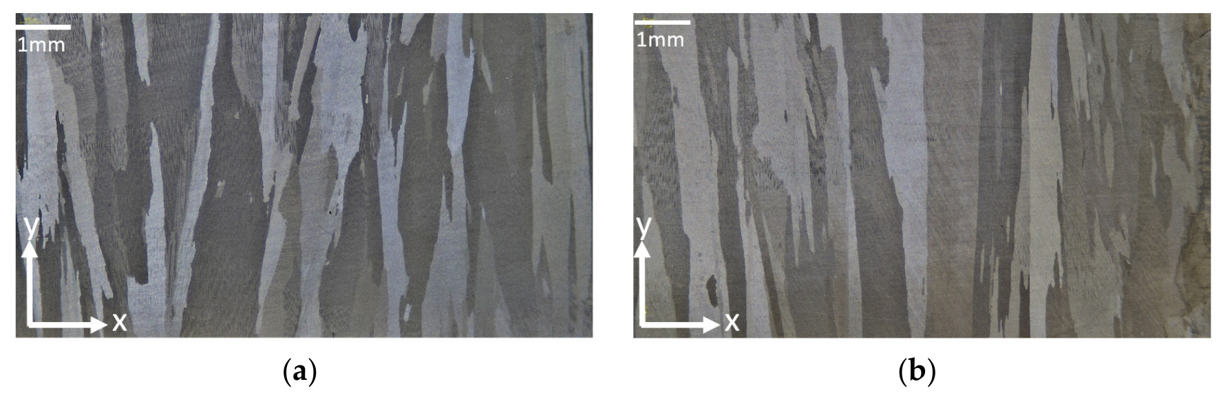
The specimen identifiers and representative microstructures of the additively manufactured pipes are shown in Figure 1. The specimens were cut from a single LPBF pipe blank (length 650 mm, outer diameter 325 mm, wall thickness 28 mm). The build direction coincides with the pipe axial direction (Y-axis in Figure 1).

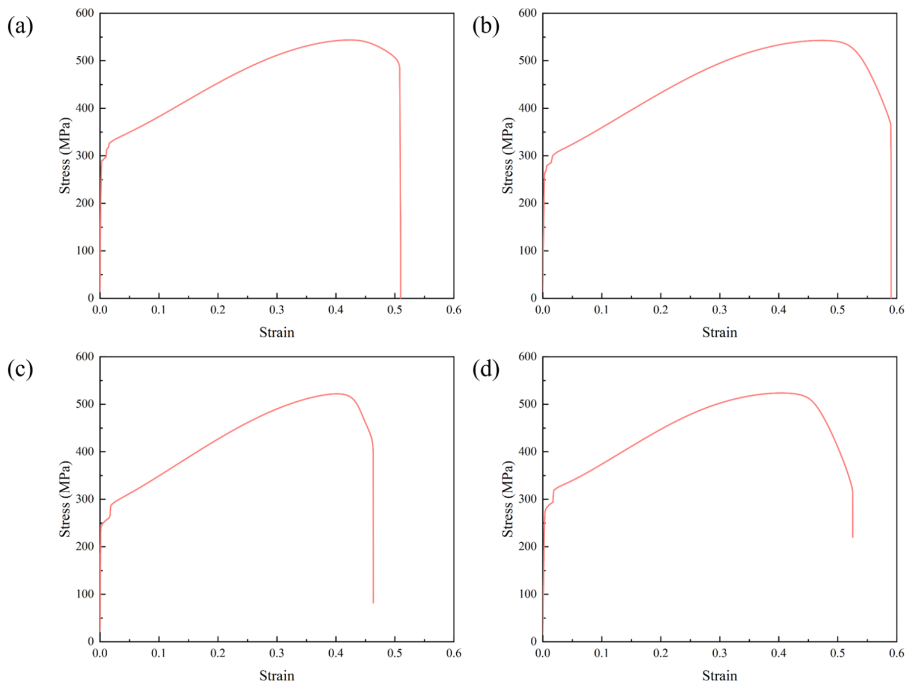
The specimen identifiers and tensile responses are summarized in Figure 2. As indicated by the figures, the circumferential and axial tensile yield strengths of specimen A were 289 and 261.5 MPa, respectively. In comparison, the corresponding values of specimen B were 245 and 278 MPa, respectively.

2.2. Experimental Tensile Response of Defect-Containing Specimens

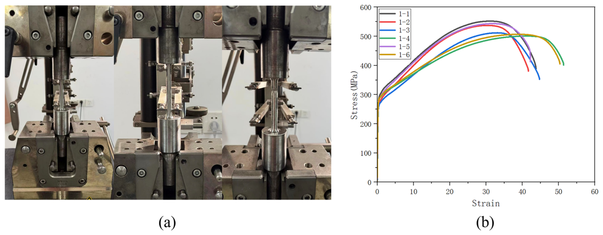
To further characterize the macroscopic mechanical response of the defect-containing material and provide an experimental basis for the subsequent numerical analysis, a series of uniaxial tensile tests was conducted on six specimens containing manufacturing defects. Before testing, each specimen was individually numbered and mounted in the grips of a universal testing machine(CMT5205, SUST, Zhuhai, China). The specimen position was carefully adjusted to ensure that its longitudinal axis was aligned with the loading direction, thereby minimizing the influence of eccentric loading. The tests were performed at room temperature under displacement control, and the load and displacement were recorded continuously throughout the loading process.

Figure 3 presents the engineering stress–strain curves of the six defect-containing specimens. All tensile curves exhibited the typical stages of elastic deformation, yielding, uniform plastic deformation, necking, and final fracture. After yielding, the engineering stress increased continuously with increasing strain, indicating pronounced strain-hardening behavior. After the ultimate tensile strength was reached, the engineering stress gradually decreased because of localized necking and progressive damage accumulation until final fracture.

The yield strengths of the six specimens were determined using the 0.2% offset method. The measured yield strengths ranged from 261.8 to 282.7 MPa, with an average value of 274.1 MPa, a standard deviation of 8.3 MPa, and a coefficient of variation of 3.0%, as listed in

Table 1. Statistical analysis of the yield strengths of six defective specimens.

Specimen Number	Yield Strength (Rp 0.2/MPa)
1–1	282.7
1–2	266.0
1–3	261.8
1–4	278.8
1–5	275.6
1–6	279.8

. Specimen 1–1 exhibited the highest yield strength of 282.7 MPa, whereas specimen 1–3 showed the lowest value of 261.8 MPa, corresponding to a difference of 20.9 MPa. Except for specimens 1–2 and 1–3, which exhibited relatively lower yield strengths, the values of the remaining specimens were concentrated within the range of 275.6–282.7 MPa. Overall, the relatively small scatter in the measured yield strengths indicates that the defect-containing specimens exhibited good consistency and repeatability in their yielding behavior. These experimental results provide a quantitative reference for the subsequent development and analysis of the crystal plasticity finite element model.

2.3. Monte Carlo Method

The Monte Carlo method discretizes the domain using a regular lattice, most commonly a hexagonal or quadrilateral lattice. The total number of lattice sites is $N_1\times N_1$. Each site has six neighbors in a hexagonal lattice and eight neighbors in a quadrilateral lattice. During initialization, each site is assigned an integer orientation value in [1, $q_1$] ($q_1$ > 1). Adjacent sites with the same orientation belong to the same grain, whereas sites with different orientations are separated by a grain boundary. A model containing $N_1\times N_1$ lattice sites is simulated over an area of $S_{\mathrm{a}}$ micrometers squared. The lattice spacing $\lambda$ is therefore calculated as $\lambda ={\displaystyle \frac{\sqrt{S_{\mathrm{a}}}}{N_1}}$. The energy of a site at a given time is defined as:

$$E_{ij}=-J_1{\displaystyle {\sum }_{i=1}^m}\left({\delta }_{q_{1i}{q}_{1j}}-1\right),$$

(1)

where $J_1$ is a positive constant representing grain-boundary energy, m is the number of neighboring sites, and $\delta$ is the Kronecker delta. Grain growth in the additively manufactured heat-affected region is represented by the coarsening of fine grains through a reduction in total grain-boundary energy and the associated migration of grain boundaries. Trial orientations are assigned iteratively and accepted or rejected according to the prescribed transition rule.

Two update schemes are commonly used. In the first, a lattice site is selected randomly and assigned an arbitrary value from [1, $q_1$]. In the second, a randomly selected site is assigned one of the orientation values of its neighbors; eight candidate values are available for a quadrilateral lattice. After a trial orientation is assigned, acceptance is evaluated using the probability as follows:

$$p_1=\{\begin{array}{c}1,\Delta E\le 0\\ e^{-{\displaystyle \frac{\Delta E}{k_{\mathrm{B}}{T}_{\mathrm{a}\mathrm{b}\mathrm{s}}}}},\Delta E>0\end{array},$$

(2)

where $p_1$ is the probability of retaining the trial orientation and $\Delta E$ is the change in total system energy; $k_{\mathrm{B}}$ is the Boltzmann constant and Tabs is the absolute temperature. A trial orientation is accepted whenever the total energy decreases. If the energy increases, it is accepted probabilistically, with the acceptance probability decreasing as the energy increment increases. Grain growth consequently evolves toward lower total energy, consistent with grain-boundary migration and reductions in temperature and dislocation density.

2.4. Crystal Plasticity Finite Element Formulation

The finite element model is constructed as a three-dimensional solid RVE with dimensions of 13 mm (circumferential, X) × 7 mm (axial, Y) × 0.1 mm (radial, Z), discretized by C3D8 elements with a uniform element size of 0.1 mm. Defects are explicitly introduced as cylindrical pores or rectangular cracks penetrating the full thickness of the RVE. The porosity is defined as the ratio of the total defect volume to the RVE total volume. For a cylindrical pore with diameter, the equivalent volume is $V={\displaystyle \frac{\pi d^2}{4}}\cdot t_{\mathrm{R}\mathrm{V}\mathrm{E}}$, where $t_{\mathrm{R}\mathrm{V}\mathrm{E}}=0.1 \mathrm{m}\mathrm{m}$. For a crack-like defect with length $l$ and width $w$, the equivalent volume is $V=l\cdot w\cdot t_{\mathrm{R}\mathrm{V}\mathrm{E}}$.

Uniaxial tensile loading was applied to the RVE under displacement control. For circumferential tension, the left surface of the RVE (X = 0) was coupled to reference point RP-1 via a kinematic coupling constraint, and RP-1 was fully fixed (U₁ = U₂ = U₃ = UR₁ = UR₂ = UR₃ = 0). The right surface (X = 13 mm) was coupled to reference point RP-2 via an identical kinematic coupling constraint, and a displacement of U₁ = 5.2 mm (ramp amplitude) was prescribed to RP-2, with all other degrees of freedom constrained (U₂ = U₃ = UR₁ = UR₂ = UR₃ = 0). Analogous boundary conditions were adopted for axial tension: the bottom surface (Y = 0) was fully fixed, and the top surface (Y = 7 mm) was subjected to a prescribed displacement in the Y-direction. All remaining external surfaces were traction-free. The kinematic coupling constraints ensured that the loaded and fixed surfaces remained planar during deformation, preventing artificial stress concentrations at the boundaries.

The total deformation gradient is multiplicatively decomposed into elastic and plastic components. Plastic deformation is assumed to arise exclusively from crystallographic slip; grain-boundary sliding and deformation twinning are neglected:

$$\mathit{F}={\mathit{F}}^{\mathrm{e}}{\mathit{F}}^{\mathrm{p}},$$

(3)

where ${\mathit{F}}^{\mathrm{e}}$ is the elastic deformation gradient associated with lattice stretching and rigid-body rotation, and ${\mathit{F}}^{\mathrm{p}}$ is the plastic deformation gradient generated by crystallographic slip. At the microscale, slip is localized within discrete slip bands rather than distributed uniformly. In a polycrystal containing many slip bands, however, the macroscopic deformation appears approximately homogeneous. Let ${\mathit{m}}^{\left(\alpha \right)}$ and ${\mathit{n}}^{\left(\alpha \right)}$ denote, respectively, the unit slip direction and slip-plane normal of slip system alpha in the intermediate configuration. Following elastic lattice deformation, ${\mathit{m}}^{\left(\alpha \right)}$ transforms to ${\mathit{m}}^{\ast \left(\alpha \right)}$, while ${\mathit{n}}^{\left(\alpha \right)}$ transforms to ${\mathit{n}}^{\ast \left(\alpha \right)}$.

$${\mathit{m}}^{\mathrm{*}\left(\alpha \right)}={\mathit{F}}^{\mathrm{e}}{\mathit{m}}^{\left(\alpha \right)}$$

(4)

$${\mathit{n}}^{\ast \left(\alpha \right)}={\left({\left({\mathit{F}}^{\mathrm{e}}\right)}^{-1}\right)}^{\mathrm{T}}{\mathit{n}}^{\left(\alpha \right)}$$

(5)

The accumulated plastic shear on the individual slip systems produces the macroscopic plastic deformation according to

$${\dot{\mathit{F}}}^{\mathrm{p}}{\left({\mathit{F}}^{\mathrm{p}}\right)}^{-1}={\displaystyle {\sum }_{\alpha =1}^N}{\dot{\gamma }}^{\left(\alpha \right)}{\mathit{m}}^{\left(\alpha \right)}\otimes {\mathit{n}}^{\left(\alpha \right)},$$

(6)

where ${\dot{\gamma }}^{\left(\alpha \right)}$ is the shear strain rate on slip system $\alpha$, and $N$ is the number of active slip systems. Thus,

$${\mathit{L}}^{\mathrm{p}}={\mathit{F}}^{\mathrm{e}}{\dot{\mathit{F}}}^{\mathrm{p}}{\left({\mathit{F}}^{\mathrm{p}}\right)}^{-1}{\left({\mathit{F}}^{\mathrm{e}}\right)}^{-1}={\displaystyle \sum _{\alpha =1}^N}{\dot{\gamma }}^{\left(\alpha \right)}{\mathit{m}}^{\ast \left(\alpha \right)}\otimes {\mathit{n}}^{\ast \left(\alpha \right)}$$

(7)

The constitutive relation is written as:

$${\widehat{\mathit{\sigma }}}^{\mathrm{e}}=\mathit{E}\mathit{M}\mathit{T}:{\mathit{D}}^{\mathrm{e}},$$

(8)

where $\mathit{E}\mathit{M}\mathit{T}$ is the elastic stiffness tensor constructed from C₁₁, C₁₂, and C₄₄, and ${\widehat{\mathit{\sigma }}}^{\mathrm{e}}$ is the Jaumann rate of the Kirchhoff stress tensor in the intermediate configuration. Therefore,

$${\widehat{\mathit{\sigma }}}^{\mathrm{e}}=\dot{\mathit{\sigma }}-{\mathit{W}}^{\mathrm{e}}\mathit{\sigma }+\mathit{\sigma }{\mathit{W}}^{\mathrm{e}}$$

(9)

For the Cauchy stress tensor in the initial configuration, the corresponding Jaumann rate is

$$\widehat{\mathit{\sigma }}=\dot{\mathit{\sigma }}-\mathit{W}\mathit{\sigma }+\mathit{\sigma }\mathit{W}$$

(10)

Consequently,

$${\widehat{\mathit{\sigma }}}^{\mathrm{e}}=\widehat{\mathit{\sigma }}+{\mathit{W}}^{\mathrm{p}}\mathit{\sigma }-\mathit{\sigma }{\mathit{W}}^{\mathrm{p}}$$

(11)

$${\mathit{W}}^{\mathrm{p}}={\displaystyle \sum _{\alpha =1}^N}{\mathit{W}}^{\left(\alpha \right)}{\dot{\gamma }}^{\left(\alpha \right)}$$

(12)

Substitution of the known variables into the constitutive relation gives

$$\widehat{\mathit{\sigma }}=\mathit{E}\mathit{M}\mathit{T}:\mathit{D}-{\displaystyle \sum _{\alpha =1}^N}\left[\mathit{E}\mathit{M}\mathit{T}:{\mathit{P}}^{\left(\alpha \right)}+{\mathit{B}}^{\left(\alpha \right)}\right]{\dot{\gamma }}^{\left(\alpha \right)}$$

(13)

Equations (1)–(11) relate the stress rate to the deformation rate and the slip-system shear rates. Specifically, the stress rate $\widehat{\mathit{\sigma }}$ depends on the shear strain rate ${\dot{\gamma }}^{\left(\alpha \right)}$ and the deformation rate $\mathit{D}$. Evaluation of the stress rate therefore requires the slip-system shear rate ${\dot{\gamma }}^{\left(\alpha \right)}$, which is obtained from ${\dot{\gamma }}^{\left(\alpha \right)}$ as follows:

$${\dot{\gamma }}^{\left(\alpha \right)}={\dot{\gamma }}^0{f}^{\left(\alpha \right)}\left({\displaystyle \frac{{\tau }^{\left(\alpha \right)}}{g^{\left(\alpha \right)}}}\right),$$

(14)

where ${\dot{\gamma }}^0$ is the reference shear strain rate, $g^{\left(\alpha \right)}$ is the slip resistance on slip system $\alpha$, ${\tau }^{\left(\alpha \right)}$ is the resolved shear stress, and $f^{\left(\alpha \right)}$ defines the stress-rate sensitivity relation:

$$f^{\left(\alpha \right)}\left(x\right)=x{\left|x\right|}^{k_1-1},$$

(15)

where $k_1$ is the rate-sensitivity exponent. As $k_1$ approaches infinity, the formulation tends toward rate-independent plasticity. Combining the preceding relations gives

$${\dot{\gamma }}^{\left(\alpha \right)}={\dot{\gamma }}^0\left({\displaystyle \frac{{\tau }^{\left(\alpha \right)}}{g^{\left(\alpha \right)}}}\right){\left|{\displaystyle \frac{{\tau }^{\left(\alpha \right)}}{g^{\left(\alpha \right)}}}\right|}^{k_1-1}$$

(16)

Strain hardening is described by the evolution equation for $g^{\left(\alpha \right)}$:

$${\dot{g}}^{\left(\alpha \right)}={\displaystyle \sum _{\beta =1}^N}{h}_{\alpha \beta }\left|{\dot{\gamma }}^{\beta }\right|$$

(17)

The summation is performed over all active slip systems, and $N$ is the number of active systems. $h_{\alpha \beta }$ is the latent-hardening modulus describing the hardening induced on slip system $\alpha$ by shear on slip system $\beta$.

$$h_{\alpha \alpha }=h\left(\gamma \right)=h_0{\mathrm{s}\mathrm{e}\mathrm{c}}^2\left|{\displaystyle \frac{h_0\gamma }{{\tau }_{\mathrm{s}}-{\tau }_0}}\right|,$$

(18)

where $h_0$ is the initial hardening modulus; ${\tau }_0$ is the initial critical resolved shear stress and equals the initial slip resistance $g^{\left(\alpha \right)}$, denoted by $g^{\left(\alpha \right)}\left(0\right)$; ${\tau }_{\mathrm{s}}$ is the saturation stress associated with large plastic deformation; and $\gamma$ is the accumulated Taylor shear strain. The self-hardening modulus $h_{\alpha \alpha }$ gives the latent-hardening modulus $h_{\alpha \beta }$ as:

$$h_{\alpha \beta }=qh\left(\gamma \right),$$

(19)

where $q$ is a material constant. A tangent-modulus scheme is introduced into the shear-strain equations to obtain the slip-system shear rates.

In the CPFE framework, the shear strain ${\gamma }^{\alpha }$, resolved shear stress ${\tau }^{\alpha }$, and accumulated shear strain $\gamma$ are defined at the slip-system level and stored in the solution-dependent state variable (STATEV) array of the UMAT subroutine. Specifically, the shear strain on the slip system is updated incrementally as ${\gamma }^{\alpha }\leftarrow {\gamma }^{\alpha }+\Delta {\gamma }^{\alpha }$ and stored in STATEV(NSLPTL + 1)–STATEV(2·NSLPTL). The resolved shear stress ${\tau }^{\alpha }$ is computed via Schmid’s law as the projection of the Cauchy stress onto the slip system, updated incrementally, and stored in STATEV(2·NSLPTL + 1)–STATEV(3·NSLPTL). The accumulated shear strain is tracked at two levels: (i) the cumulative shear strain on each individual slip system, ${\gamma }_{\mathrm{i}\mathrm{n}\mathrm{d}}^{\alpha }={\int }_0^t\left|{\dot{\gamma }}^{\alpha }\right|dt$, stored in STATEV(9·NSLPTL + 1)–STATEV(10·NSLPTL), and (ii) the total cumulative shear strain over all slip systems, ${\gamma }_{\mathrm{t}\mathrm{o}\mathrm{t}}={\sum }_{\alpha =1}^N{\int }_0^t\left|{\dot{\gamma }}^{\alpha }\right|dt$, stored in STATEV(10·NSLPTL + 1). All three quantities are field variables defined at each Gauss integration point. The mean shear strain, mean resolved shear stress, and mean accumulated shear strain reported in the following sections are obtained by volume-averaging the corresponding field variables over all Gauss integration points within the RVE.

3. Results and Discussion

3.1. Validation of the Monte Carlo Reconstruction

The experimentally observed microstructure was reconstructed using the Monte Carlo method by prescribing the sampling domain and grain-growth probability. Grain orientations, dimensions, and spatial positions were generated through simulated grain growth, and the resulting morphology and orientation data were transferred to the CPFE model. The Monte Carlo geometry was discretized into a finite element mesh and assigned the corresponding crystal orientations. Reaction force–displacement curves were extracted to obtain the local mechanical response and were compared with the tensile measurements to validate the micromechanical framework.

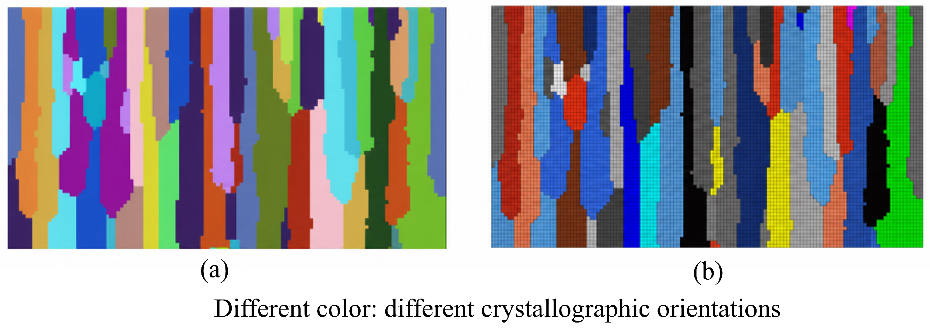
The reconstructed and experimentally observed microstructures were compared in Figure 4. The analyzed region measured 13 × 7 mm and corresponded to specimen A. The microstructure was dominated by columnar grains. The experimentally measured columnar-grain width was 0.52 mm, whereas the Monte Carlo model predicted 0.50 mm, corresponding to an error of 3.8%. A finite element mesh was subsequently generated from the reconstructed morphology, as shown in Figure 4b.

3.2. Validation of the Crystal Plasticity Model

3.2.1. Defect-Free Model

The crystal plasticity parameters were calibrated against the experimental stress–strain curves (

Table 2. Crystal plasticity parameters for 316L stainless steel.

Material Parameter	Value
C11 (GPa)	204.6
C12 (GPa)	137.7
C44 (GPa)	126.2
h0 (MPa)	171
τs (MPa)	214
τ0 (MPa)	116
k1	55
${\dot{\gamma }}_0$(s−1)	0.001

). The initial orthotropic elastic constants for 316L stainless steel were C₁₁ = 204.6 GPa, C₁₂ = 137.7 GPa, and C₄₄ = 126.2 GPa, as used in Equation (6). The rate-sensitivity exponent was k₁ = 55 for Equation (13), and the reference strain rate was 0.001 s⁻¹. The three parameters governing post-yield stiffness, saturation strength, and initial yielding were inversely identified from the defect-free experimental response: initial hardening modulus is h₀ = 171 MPa, the saturation stress is τ_s = 214 MPa, and the initial critical resolved shear stress is τ₀ = 116 MPa. These values were used in Equation (16) and retained for the subsequent defect-containing simulations.

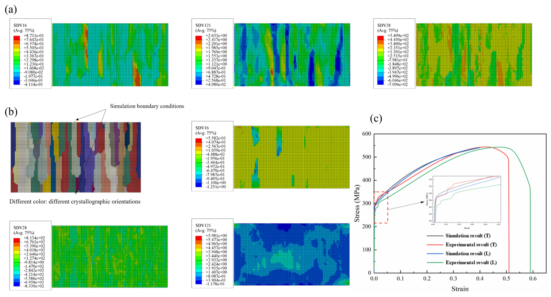
The simulation results are summarized in Figure 5. The circumferential-tension response of the defect-free model is shown in Figure 5a. The face-centered cubic 316L stainless steel contains 12 slip systems. Taking the (−1 1 1) [1 0 1] system as an example, the resolved shear stress is the projection of the applied stress onto the slip direction and plane, whereas the slip-system shear strain is obtained by integrating the slip rate. These quantities reveal the local, nonuniform activation of individual systems that is obscured in conventional continuum stress and strain contours. The mean shear strain and resolved shear stress on the selected slip system were 0.016 and 340 MPa, respectively, and the mean accumulated shear strain was 0.257.

The boundary conditions and computed axial-tension response are shown in Figure 5b. The mean shear strain, resolved shear stress, and accumulated shear strain were −0.346, 264.6 MPa, and 0.390, respectively. Figure 5c compares the predicted and measured tensile stress–strain curves. As indicated by the figure, the CPFE model predicted circumferential and axial yield strengths of 294.3 and 286.9 MPa, respectively, compared with measured values of 289 and 261.5 MPa. The corresponding errors were 1.8% and 9.7%, demonstrating that the model captures the principal anisotropic yielding response.

3.2.2. Defect-Containing Model

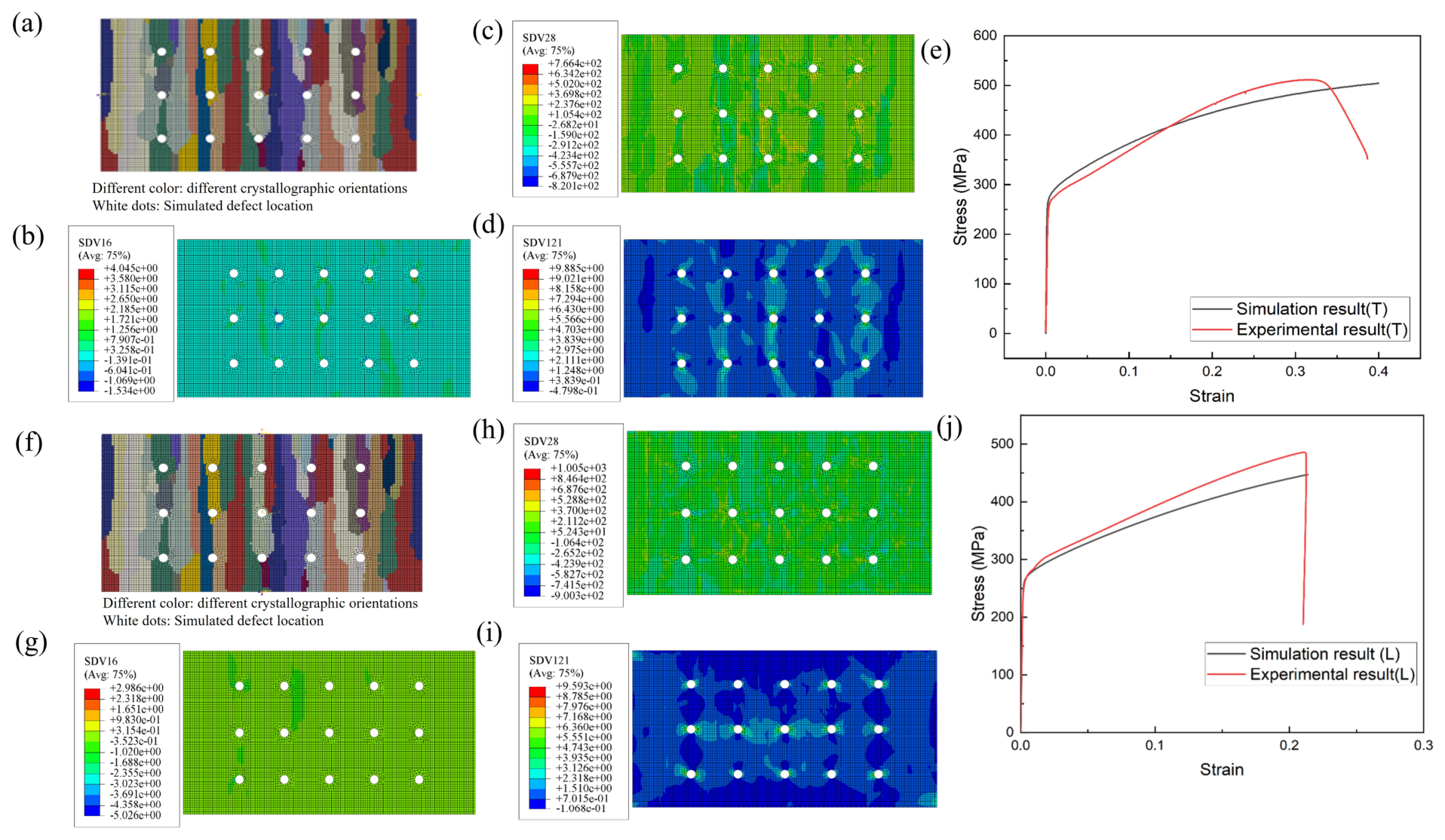
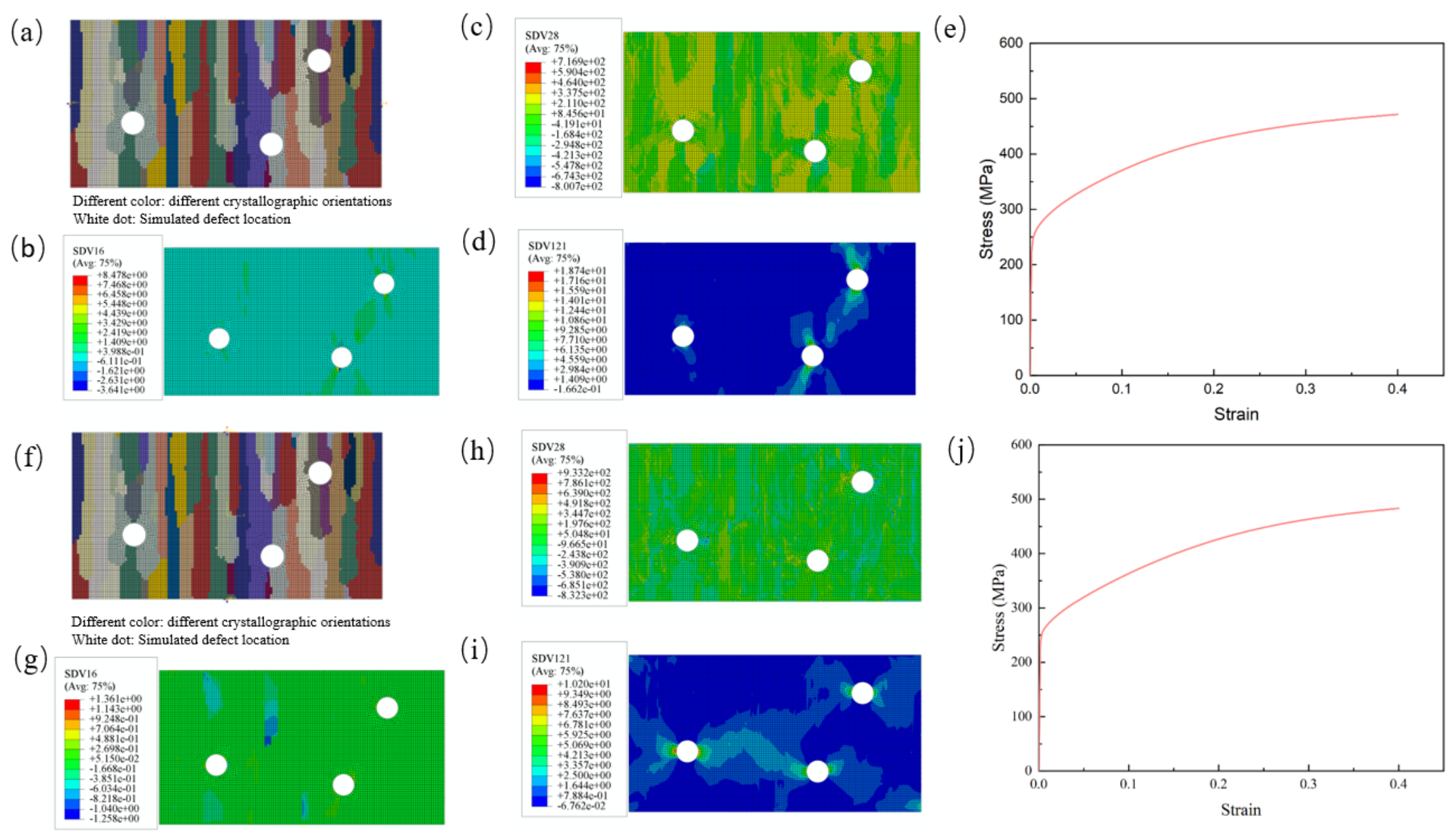
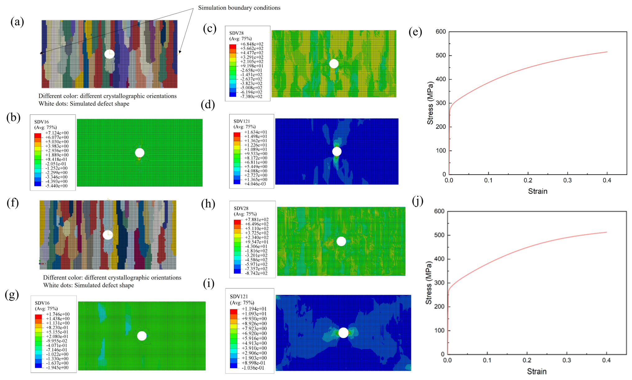
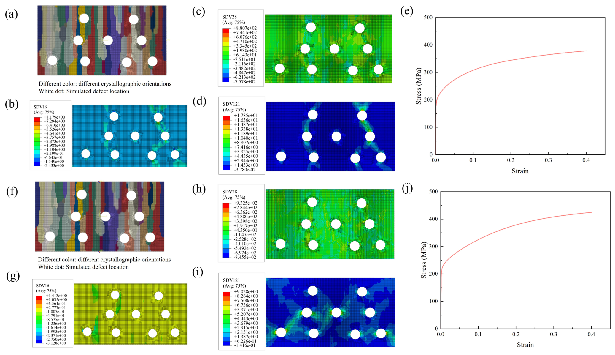
Pores or cracks were introduced into the calibrated defect-free model. Fifteen pores with a diameter of 0.4 mm were added, resulting in a porosity of 2.1%. The circumferential-tension boundary conditions and results are shown in Figure 6a–d. The mean shear strain, resolved shear stress, and accumulated shear strain were 0.139, 369.8 MPa, and 0.384, respectively. As shown in Figure 6e, the predicted circumferential yield strength was 272.9 MPa, compared with the measured value of 261.8 MPa, giving a relative error of 4.2%.

The axial-tension boundary conditions and results are shown in Figure 6f–i. The mean shear strain, resolved shear stress, and accumulated shear strain were −0.352, 370 MPa, and 0.702, respectively. Figure 6j compares the predicted and measured curves. The calculated axial yield strength was 267.7 MPa, compared with the experimental value of 265.5 MPa, corresponding to an error of 0.8%.

3.3. Defect-Shape Sensitivity

After validation, the model was further used to quantify the effects of two representative defect classes, pores and cracks. Pore diameter, crack length, pore arrangement, and porosity were varied, and their effects on circumferential and axial yielding were evaluated using the stress–strain response, yield strength, slip-system shear strain, resolved shear stress, and accumulated shear strain. Defects of specific shapes, sizes, porosities, and arrangements were considered to quantitatively reveal the governing mechanisms of defect-induced yield degradation. The combined macroscopic and local-field results clarify the mechanisms governing defect-induced degradation.

Defect shape governs both the local stress-concentration pattern and the reduction in effective load-bearing area. A circular pore primarily produces stress concentration around its boundary, whereas a crack is directional and contains sharp tips that promote localized deformation and potential failure paths. A pore of 1 mm diameter and a crack of 4 mm long and 0.1 mm wide were therefore selected as representative defects for comparison under circumferential and axial tension.

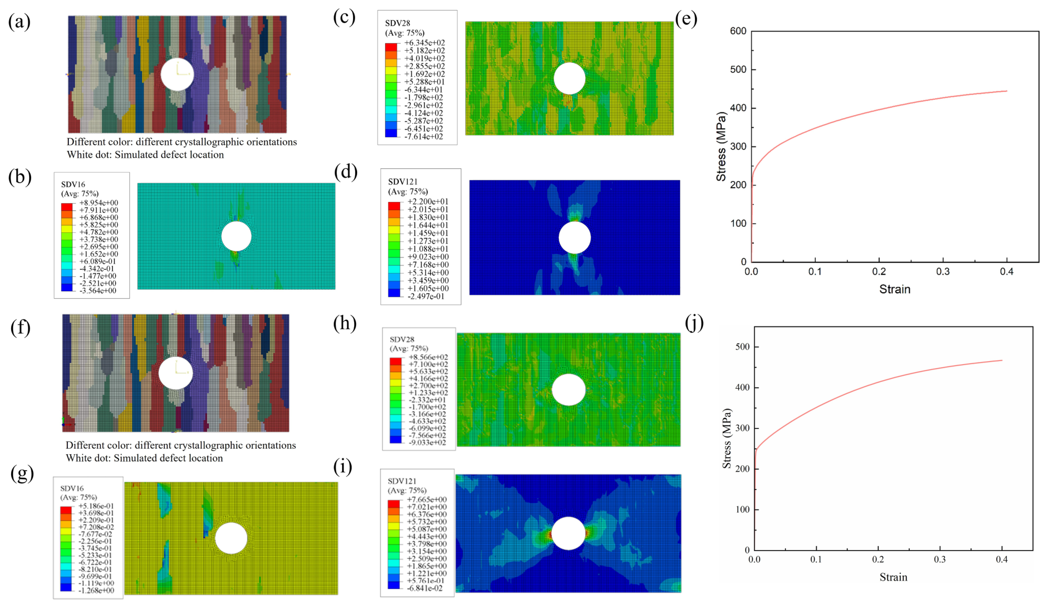
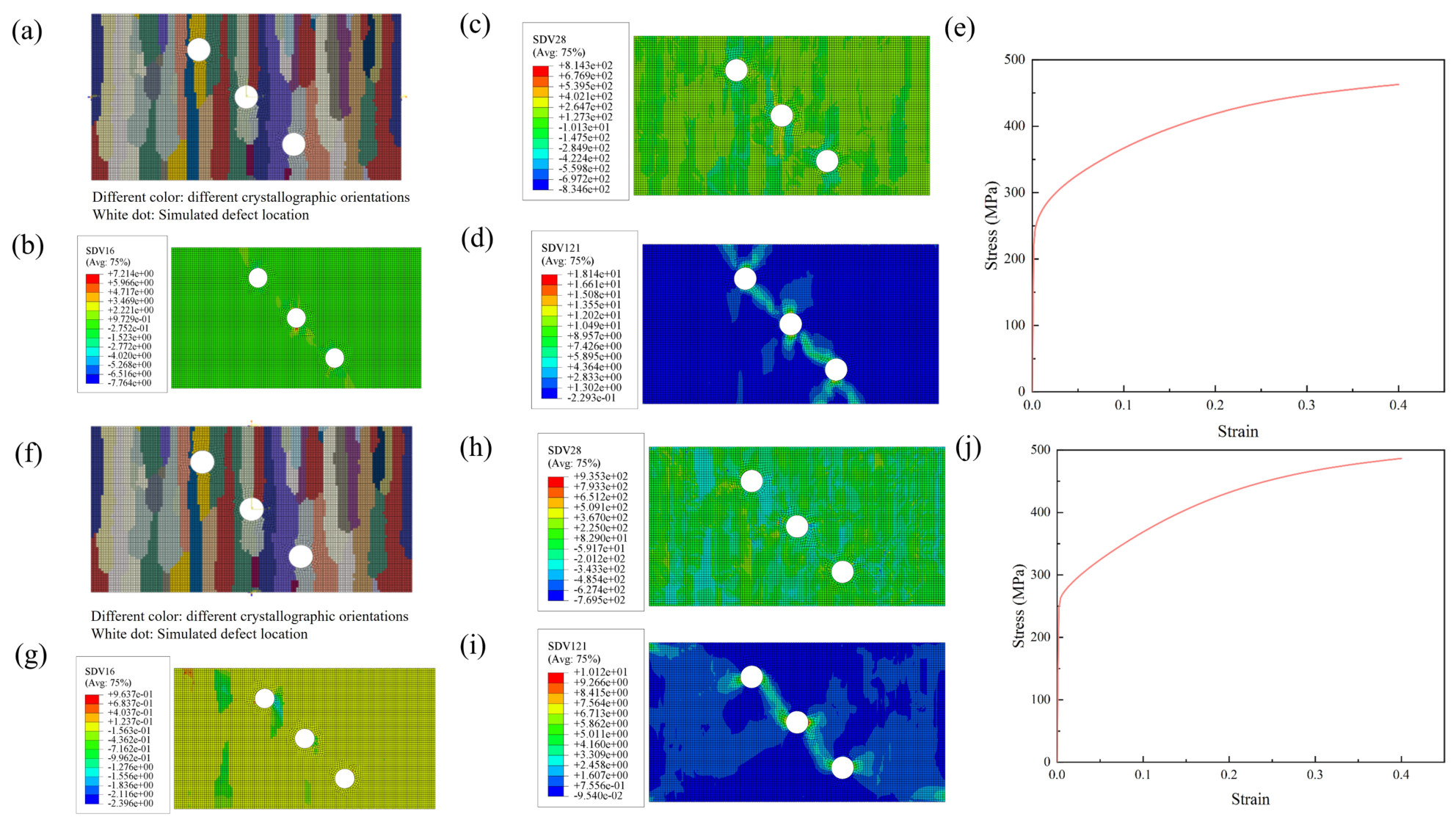
The local stress and strain fields and stress–strain curves for the model with a pore of diameter 1 mm are shown in Figure 7. The circumferential and axial yield strengths were 282.5 and 272.3 MPa, respectively, both lower than those of the defect-free model. Shear strain and accumulated shear strain were localized around the pore boundary, indicating that the geometric discontinuity redistributes stress and triggers early plastic deformation. The reduction in strength is therefore attributable to both loss of effective load-bearing area and pore-edge stress concentration.

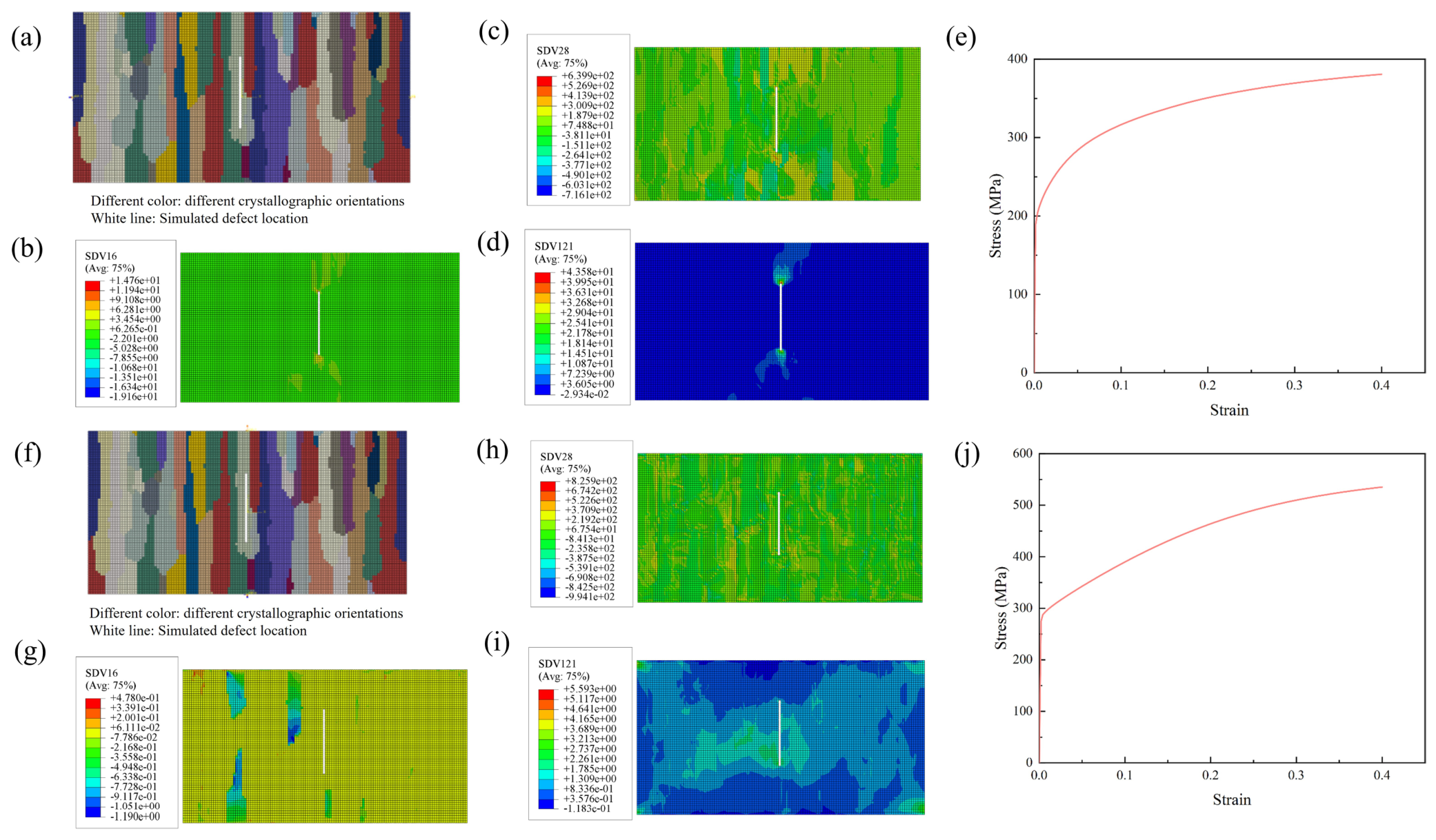
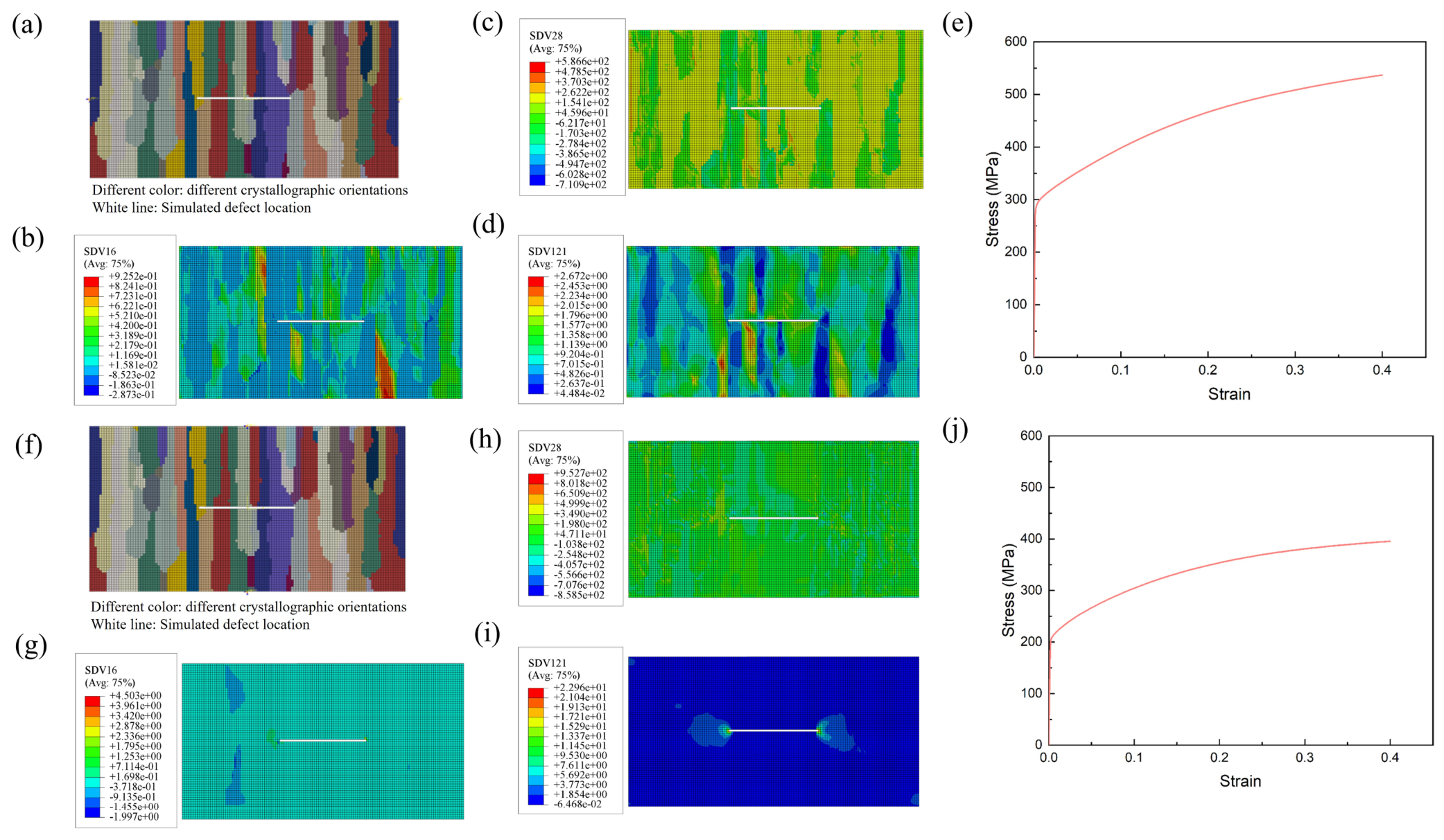
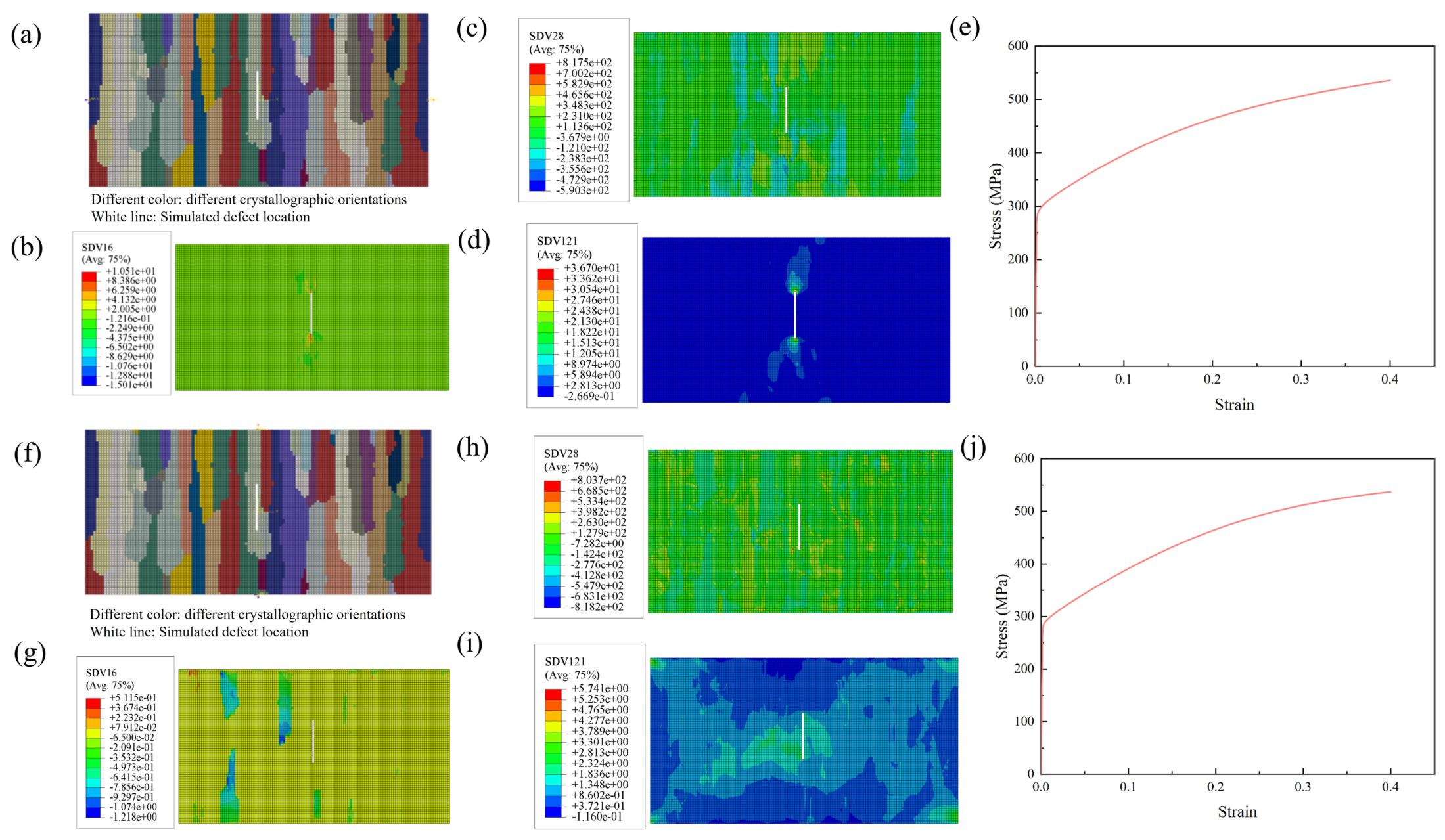
The responses of the model with a crack of 4 mm width are presented in Figure 8. In contrast to the pore, the crack showed pronounced directional sensitivity. Under circumferential tension, the yield strength was 292 MPa and remained close to the defect-free value, indicating limited influence for this crack orientation. Under axial tension, however, the yield strength decreased to 209.2 MPa. Strong stress and accumulated shear strain developed near the crack tips. When the crack orientation was unfavorable relative to the loading direction, the effective load path was disrupted, and plastic deformation was localized at the crack tips.

As indicated by the above discussion, both defect types reduced the yield strength, but through different mechanisms. Pores produced a comparatively uniform reduction through edge stress concentration and loss of load-bearing area. Cracks exhibited a strongly directional effect controlled by their orientation relative to the applied load. Defect-tolerance assessments should therefore emphasize pore size and porosity for pore-like defects, while jointly considering crack length and orientation for crack-like defects.

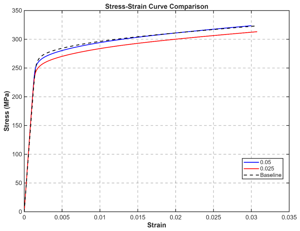
To evaluate the sensitivity of the predicted mechanical response to mesh density, the 1 mm pore model introduced above was selected as the baseline case. Two element sizes, namely 0.05 mm and 0.025 mm, were employed to discretize the same baseline geometry under uniaxial tension, and the predicted stress–strain curves were compared with the baseline solution in Figure 9. As indicated by the figure, the elastic moduli predicted by the 0.05 mm and 0.025 mm meshes are approximately 183.6 GPa and 182.9 GPa, respectively, which deviate from the baseline value of 176.0 GPa by 4.4% and 4.0%. The nearly identical elastic moduli obtained from the two meshes indicate that the elastic response is already mesh-converged at the 0.05 mm resolution.

In the yield-transition regime, the 0.05 mm mesh produced stress values that agree with the baseline data within a relative error of 0.01–4.4%, with the deviation diminishing to 0.11% at larger strains. The 0.025 mm mesh yielded a comparable level of agreement, with relative deviations ranging from 3.1% to 5.0%. The marginal difference between the two mesh predictions—only 0.4% in elastic modulus and within 2% in flow stress at identical strain levels—demonstrates that halving the element size exerts a limited influence on the macroscopic stress–strain response under the present crystal-plasticity framework. Both discretization sizes captured the baseline trend with comparable fidelity, confirming that the defect-size and defect-distribution investigations presented in the preceding sections are not subject to significant mesh-induced bias.

3.4. Defect-Size Sensitivity

Defect size is a key parameter in defect-tolerance assessment. Increasing pore diameter reduces the effective load-bearing area and intensifies stress concentration at the pore boundary, potentially lowering the yield strength and initiating local plasticity at an earlier stage. Models containing pores of different diameters were therefore systematically analyzed under circumferential and axial tension to reveal the defect-size sensitivity.

3.4.1. Size of Pore

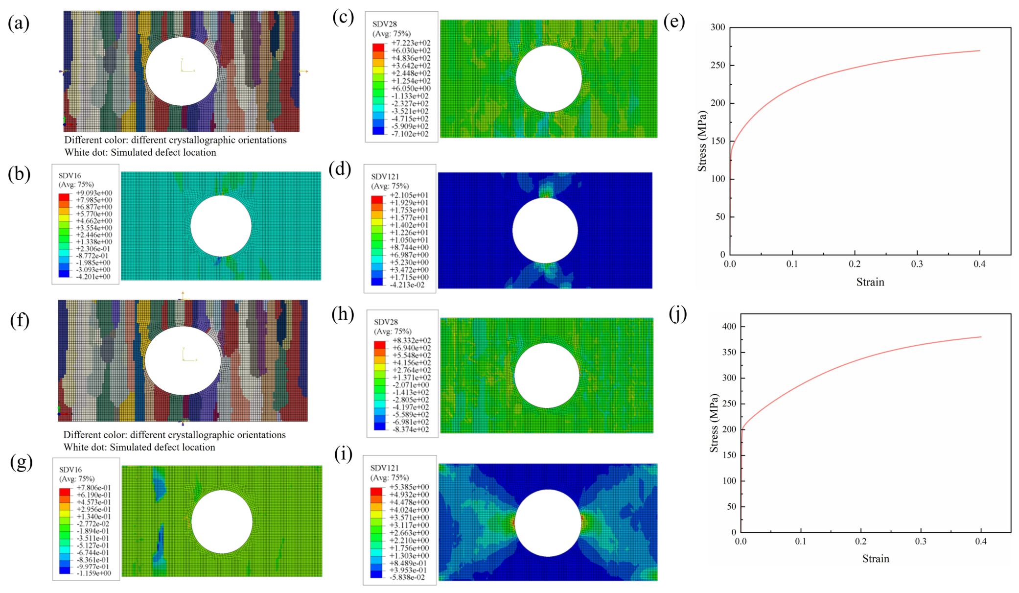
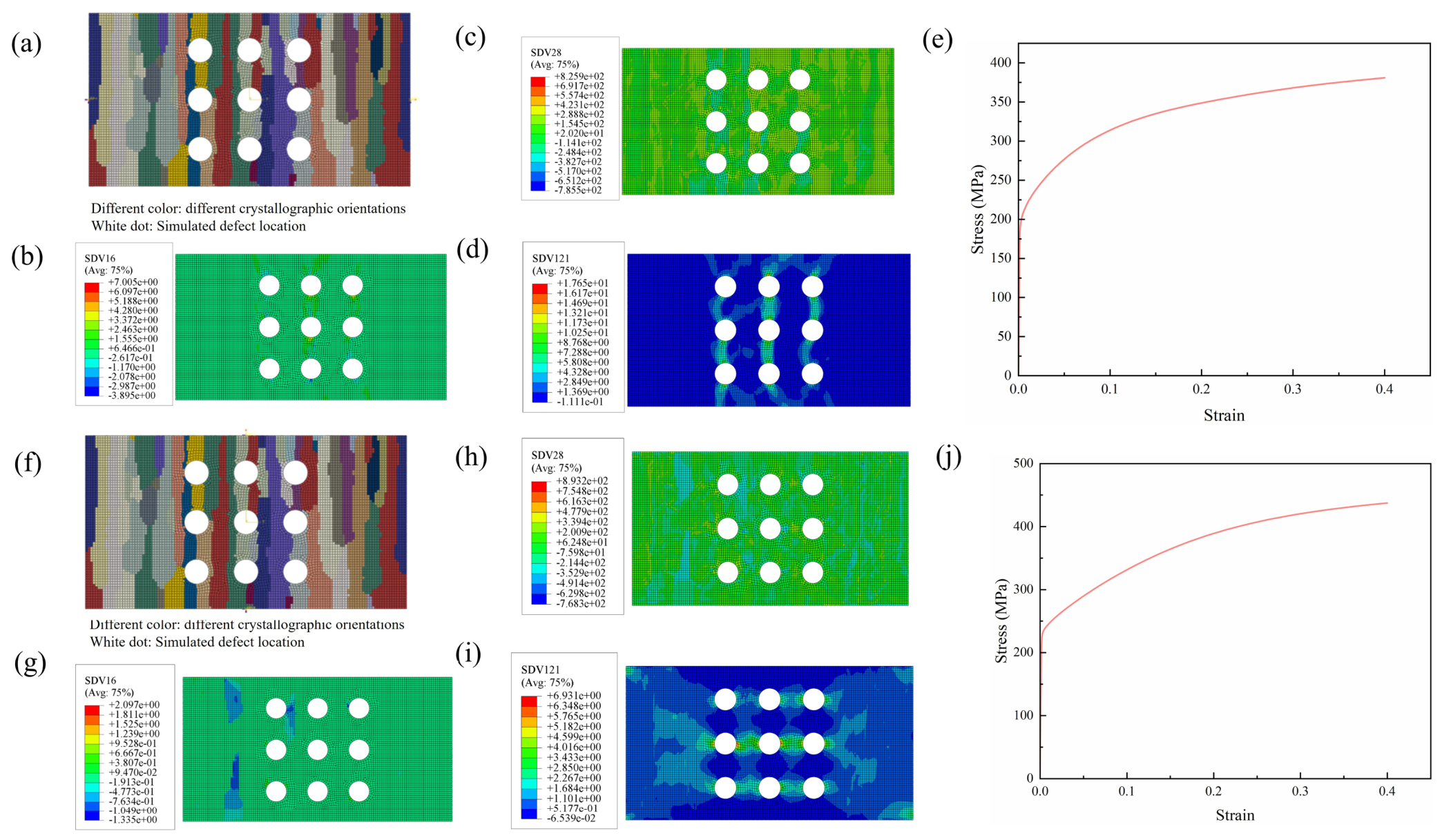
The pore diameters of 2 and 4 mm were modeled under the same conditions and compared with the 1 mm case, which are shown in Figure 10 and Figure 11 respectively. As indicated by the figures, the yield strength decreased markedly with increasing pore size. For diameters of 2 and 4 mm, the circumferential yield strengths decreased to 234.6 and 140.1 MPa, respectively, while the axial values decreased to 248.3 and 204.03 MPa. Moreover, the circumferential response was more sensitive to pore diameter. Larger pores also expanded the regions of concentrated shear strain and accumulated shear strain. The associated reduction in effective area and stronger pore-edge stress concentration accelerated earlier local plastic deformation, identifying large pores as a critical source of strength degradation.

3.4.2. Sizes of Circumferential Cracks

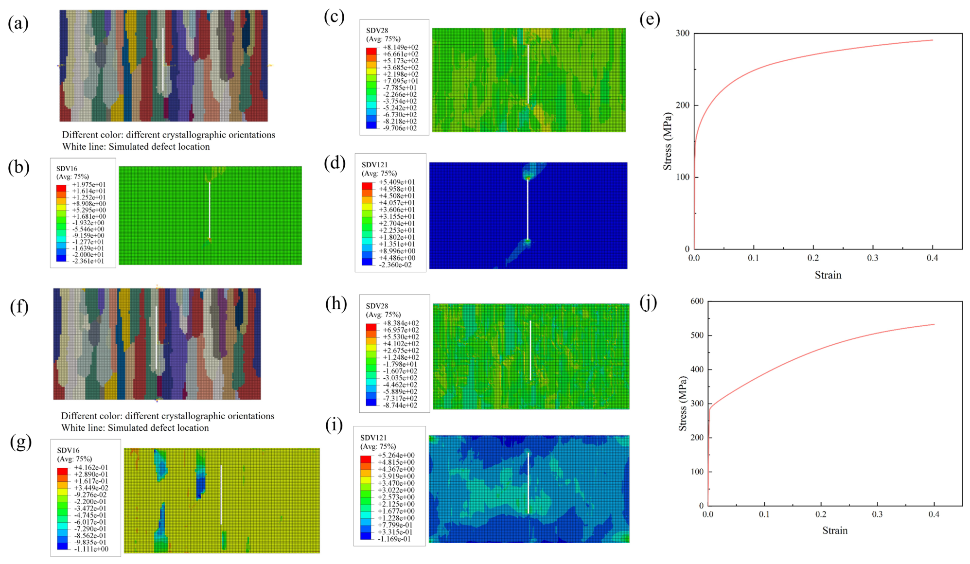
To investigate the effects of the crack width on the mechanical responses of the additively manufactured structures, the circumferential cracks with lengths of 6 and 8 mm were modeled in addition to the 4 mm case. Both loading directions were analyzed and the results are shown in Figure 12 and Figure 13. The circumferential yield strengths for the models with 6 and 8 mm cracks were 292.5 and 288.1 MPa, respectively, showing little change with the variation in the crack length. In contrast, the axial yield strengths decreased sharply to 166.4 and 121 MPa. Under axial loading, stress and accumulated shear strain localized near the crack tips, demonstrating that circumferential cracks reduce the effective axial load-bearing section and promote tip-localized plastic deformation. Their adverse effect on axial capacity increased substantially with crack length.

3.4.3. Length of Axial Cracks

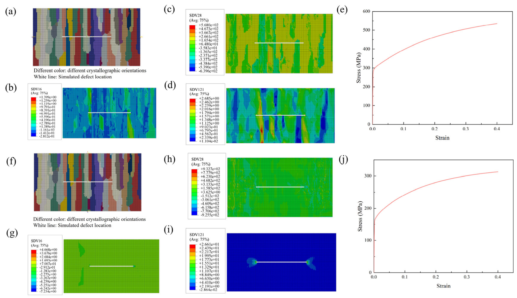
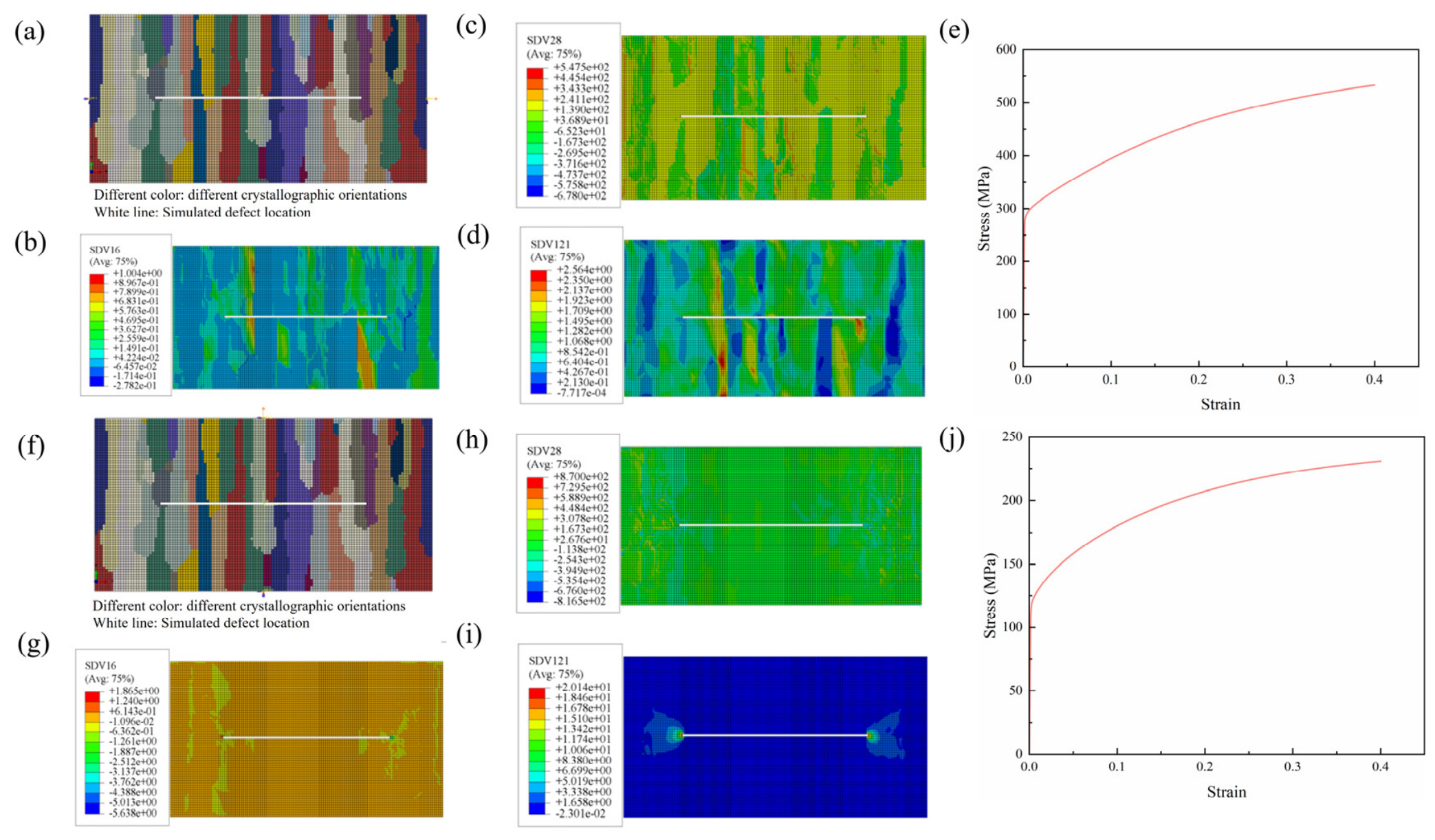
To further investigate the effects of the size of the axial cracks, the cracks with lengths of 2, 3, and 4 mm were modeled under identical circumferential and axial loading conditions. The resulting responses are presented in Figure 14, Figure 15 and Figure 16. As shown by the figures, the circumferential yield strength decreased from 291.2 to 200.1 and 153.1 MPa as axial crack length increased from 2 to 4 mm. The corresponding axial yield strengths were 287.8, 285.9, and 285.6 MPa, exhibiting only minor variation. Therefore, the axial cracks strongly impair circumferential capacity but have limited influence on axial capacity. Under circumferential tension, stress and accumulated shear strain concentrated near the crack tips, indicating the disruption of the effective circumferential load path and preferential development of local plasticity. Under axial tension, the crack was approximately parallel to the loading direction and caused much less disruption of the principal load path, leaving the axial yield strength nearly unchanged.

In summary, the combined results confirm a clear loading-direction selectivity; that is, the circumferential cracks primarily reduce axial capacity, whereas axial cracks primarily reduce circumferential capacity. Crack length and orientation must therefore be treated as coupled variables in defect-tolerance assessment.

3.5. Distribution of the Defects

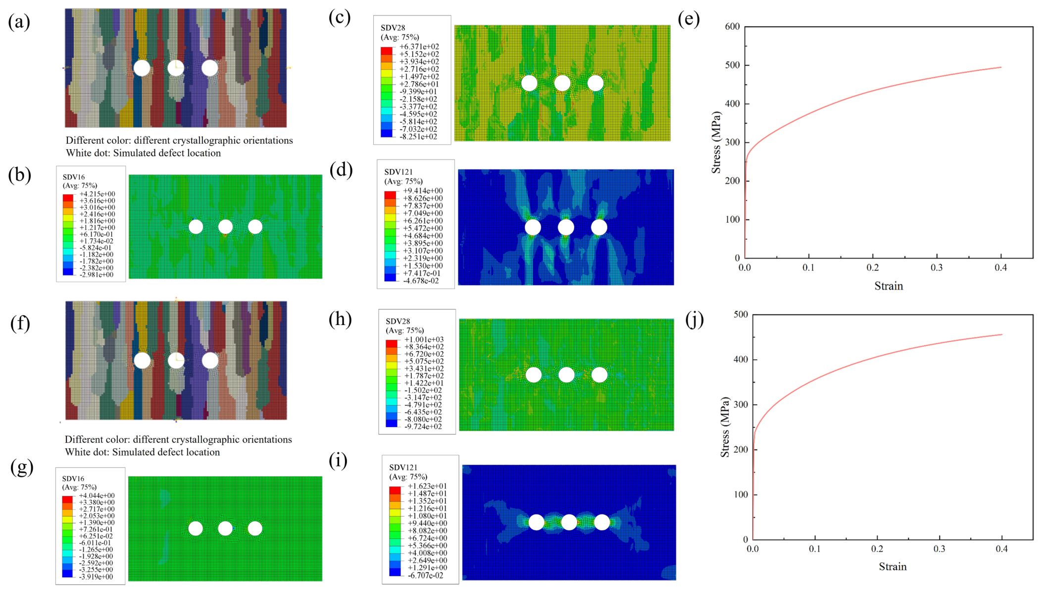
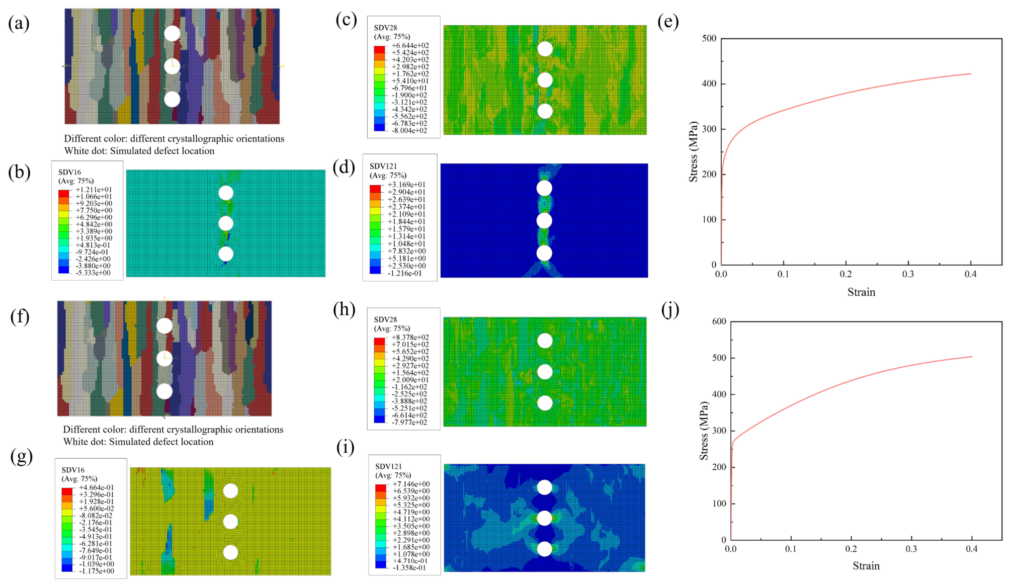
In additively manufactured materials, pores generally occur as populations rather than isolated defects. Their spatial arrangement governs interactions among local stress-perturbation fields and can alter the anisotropic mechanical response. To investigate the influences of the distribution of defects, models with circumferential, axial, and 45-degree diagonal pore arrangements at a constant porosity were analyzed under both loading directions and the results are shown in Figure 17, Figure 18 and Figure 19.

As indicated by the figures, the circumferentially arranged model produced circumferential and axial yield strengths of 262.5 and 240.5 MPa, respectively. The axially arranged model produced 227.8 and 267.6 MPa, while the 45-degree arrangement produced 247.7 and 260.5 MPa. Circumferential arrangements therefore caused a larger reduction in axial strength, whereas axial arrangements caused a larger reduction in circumferential strength. The diagonal arrangement affected both directions and yielded intermediate values. Thus, directional pore arrays modified the load-transfer path and coupled the stress-concentration zones of neighboring pores. When the pore alignment was unfavorable relative to the principal load path, local plastic zones were more likely to coalesce, leading to a pronounced decrease in yield strength. Taken together, the pore arrangement controlled both the magnitude and directionality of strength degradation.

3.5.1. Effect of Porosity

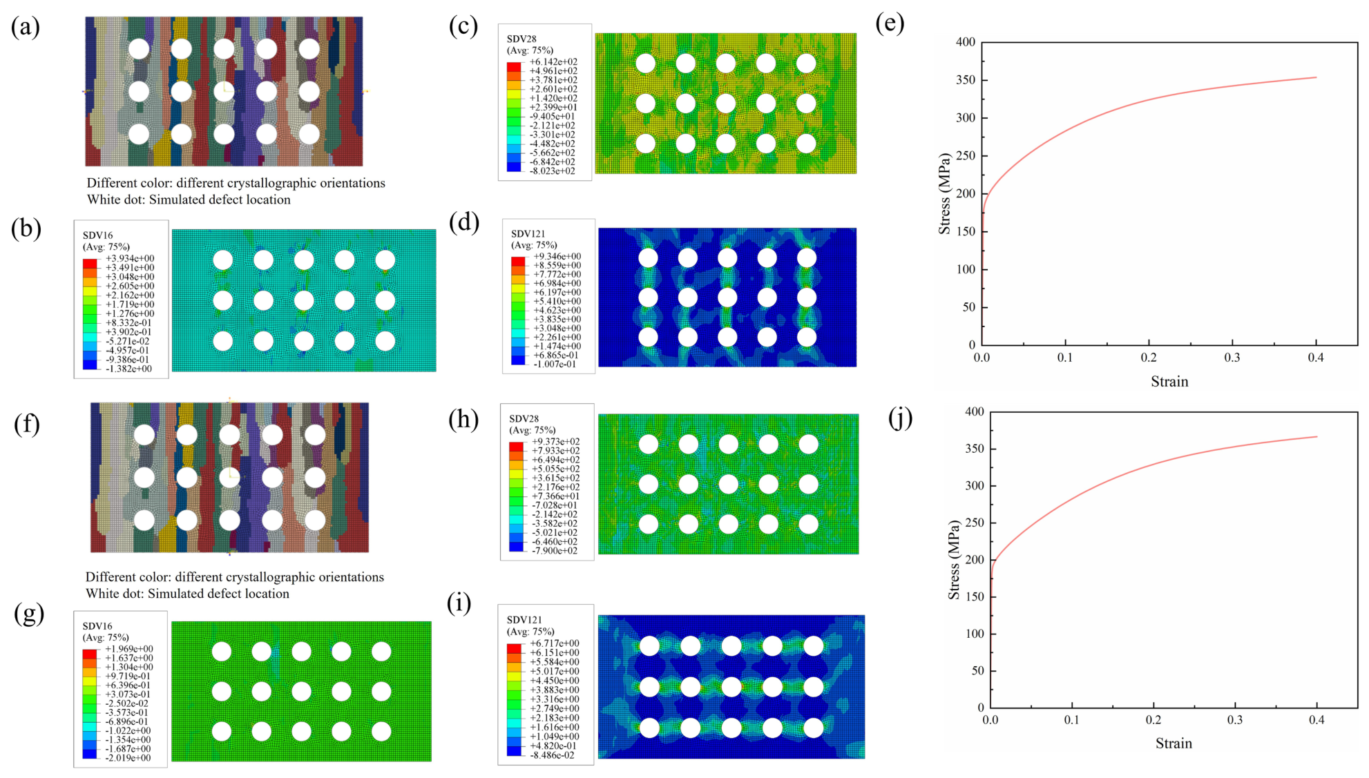
To quantify the cumulative effect of pore populations, the number of pores was increased to obtain porosities of 7.8% and 12.9%. The corresponding results are shown in Figure 20 and Figure 21. As indicated by the figures, the yield strength decreased in both directions as porosity increased. At 7.8% porosity, the circumferential and axial yield strengths were 202.2 and 233.6 MPa, respectively. At a porosity of 12.9%, the circumferential and axial yield strengths decreased by 36.4% and 32.5%, respectively, relative to those of the defect-free model. The greater degradation at high porosity demonstrates a pronounced cumulative damage effect. This can be explained by the increasing porosity expanding the regions of concentrated shear strain and accumulated shear strain and promoting interactions among the plastic zones surrounding adjacent pores. At a low porosity, the local stress perturbations remained relatively independent; at a high porosity, they coupled and substantially reduced the overall load-bearing capacity. Thus, the pore arrangement primarily controlled the directionality of degradation, whereas porosity governed the cumulative defect effect. Therefore, assessment of additively manufactured pipe materials should consider the spatial arrangement and total concentration of pores in addition to the size of individual defects.

3.5.2. Random Pore Arrangements

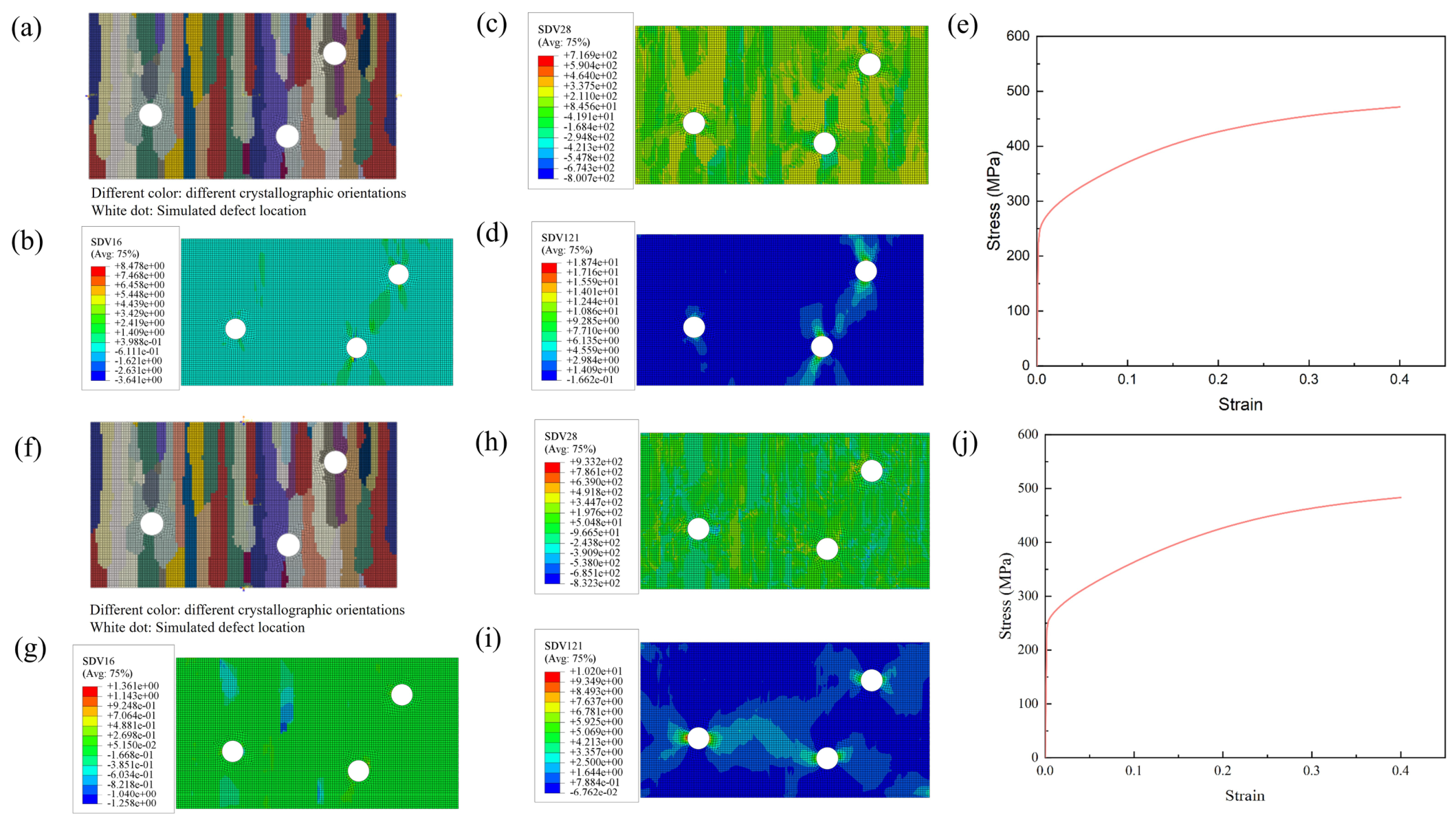
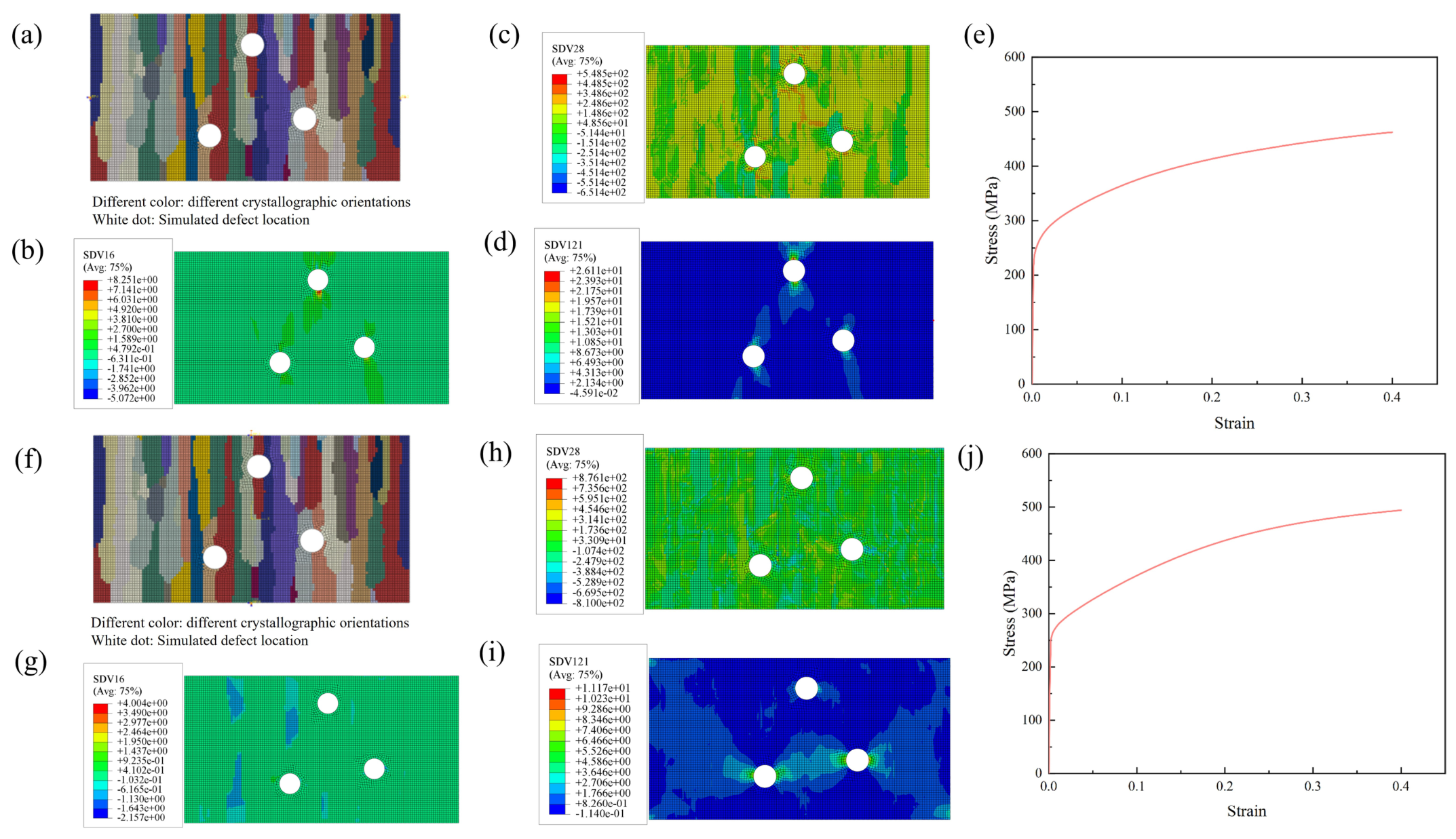
At a fixed porosity of 2.6%, three random configurations were generated, each containing three pores with a diameter of 1 mm. These models were used to evaluate the influence of random spatial arrangement on macroscopic strength and local plasticity. The simulation results are shown in Figure 22, Figure 23 and Figure 24. As indicated by the figures, the three configurations produced circumferential yield strengths of 249.7, 247.7, and 244.3 MPa and axial yield strengths of 253.1, 260.3, and 259.9 MPa. The limited scatter indicates that changes in relative pore position alter the degree of local stress-field interaction, but the macroscopic response remains statistically stable over the configurations considered. The locations of concentrated shear strain and accumulated shear strain differed among the random models, confirming that pore position controls the local plastic-deformation path. Moreover, compared to directional arrangements, randomization reduced strong anisotropy and brought the circumferential and axial yield strengths closer together, producing a quasi-isotropic response.

A random model at 7.8% porosity was further compared with the uniformly distributed model at the same porosity (Figure 25). The random model produced circumferential and axial yield strengths of 198.9 and 220.1 MPa, respectively, both lower than those with the uniform-distribution pores. In addition, at higher porosity, random placement more readily formed local defect clusters, intensifying interactions among stress-concentration and plastic zones and further reducing load-bearing capacity. Therefore, random pore distributions have two principal effects: individual configurations introduce limited scatter in local fields and yield strength, while their macroscopic response remains relatively stable at a fixed porosity. As the porosity increases, local clustering becomes more pronounced and may produce greater degradation than a uniform arrangement. The above simulation results suggest that practical defect assessments should consequently account for both porosity and spatial randomness.

4. Conclusions

Based on experimental microstructural observations, Monte Carlo grain reconstruction, and crystal plasticity finite element modeling, this study established a micromechanical framework for analyzing defects in additively manufactured 316L stainless-steel pipe material. The defect sensitivity of size, orientation, concentration, and spatial distribution on the yielding behavior were quantitatively identified. The main conclusions are as follows:

• An experimentally informed MC–CPFEM framework was developed to reconstruct the columnar-grained microstructure and predict the mechanical response of defect-containing material. The reconstruction error in the columnar-grain width was 3.8%, while the maximum errors in the predicted yield strengths of the defect-free and pore-containing models were 9.7% and 4.2%, respectively. This confirms the accuracy of the developed micromechanical framework.
• Pore size and crack orientation were identified as the primary factors governing strength degradation. Increasing pore size caused progressively greater reductions in the circumferential and axial yield strengths, with maximum decreases of 52.4% and 28.9%, respectively. Circumferential cracks primarily reduced the axial load-bearing capacity, whereas axial cracks mainly reduced the circumferential capacity, with maximum strength reductions of 57.8% and 48.0%, respectively.
• Pore distribution governed the directionality of strength degradation, whereas pore concentration controlled the overall damage level. At a pore concentration of 2.6%, directional pore arrangements produced the greatest strength reduction in the loading direction perpendicular to the pore alignment, while random distributions reduced the difference between the circumferential and axial strengths. When the pore concentration increased to 12.9%, the yield-strength reductions in both directions exceeded 30%.

References

1. Narasimharaju, S.R.; Zeng, W.; See, T.L.; Zhu, Z.; Scott, P.; Jiang, X.; Lou, S. A comprehensive review on laser powder bed fusion of steels: Processing, microstructure, defects and control methods, mechanical properties, current challenges and future trends. J. Manuf. Process. 2022, 75, 375–414. [Google Scholar] [CrossRef]
2. Kotadia, H.R.; Gibbons, G.; Das, A.; Howes, P.D. A review of laser powder bed fusion additive manufacturing of aluminium alloys: Microstructure and properties. Addit. Manuf. 2021, 46, 102155. [Google Scholar] [CrossRef]
3. Martucci, A.; Aversa, A.; Lombardi, M. Ongoing challenges of laser-based powder bed fusion processing of Al alloys and potential solutions from the literature—A review. Materials 2023, 16, 1084. [Google Scholar] [CrossRef] [PubMed]
4. Su, J.-L.; Jiang, F.-L.; Teng, J.; Chen, L.-Q.; Requena, G.; Yan, M.; Zhang, L.-C.; Wang, Y.M.; Okulov, I.V.; Zhu, H.-M.; et al. Laser additive manufacturing of titanium alloys: Process, materials and post-processing. Rare Met. 2024, 43, 6288–6328. [Google Scholar] [CrossRef]
5. Dejene, N.D.; Lemu, H.G. Current status and challenges of powder bed fusion-based metal additive manufacturing: Literature review. Metals 2023, 13, 424. [Google Scholar] [CrossRef]
6. Grilli, N.; Hu, D.; Yushu, D.; Chen, F.; Yan, W. Crystal plasticity model of residual stress in additive manufacturing using the element elimination and reactivation method. Comput. Mech. 2022, 69, 825–845. [Google Scholar] [CrossRef]
7. Hu, D.; Grilli, N.; Yan, W. Dislocation structures formation induced by thermal stress in additive manufacturing: Multiscale crystal plasticity modeling of dislocation transport. J. Mech. Phys. Solids 2023, 173, 105235. [Google Scholar] [CrossRef]
8. Kan, W.H.; Chiu, L.N.S.; Lim, C.V.S.; Zhu, Y.; Tian, Y.; Jiang, D.; Huang, A. A critical review on the effects of process-induced porosity on the mechanical properties of alloys fabricated by laser powder bed fusion. J. Mater. Sci. 2022, 57, 9818–9865. [Google Scholar] [CrossRef]
9. Huang, Y.; Fleming, T.G.; Clark, S.J.; Marussi, S.; Fezzaa, K.; Thiyagalingam, J.; Leung, C.L.A.; Lee, P.D. Keyhole fluctuation and pore formation mechanisms during laser powder bed fusion additive manufacturing. Nat. Commun. 2022, 13, 1170. [Google Scholar] [CrossRef] [PubMed]
10. Yang, X.; Li, Y.; Li, B. Formation mechanisms of lack of fusion and keyhole-induced pore defects in laser powder bed fusion process: A numerical study. Int. J. Therm. Sci. 2023, 188, 108221. [Google Scholar] [CrossRef]
11. Frieden Templeton, W.; Hinnebusch, S.; Strayer, S.T.; To, A.C.; Pistorius, P.C.; Narra, S.P. A mechanistic explanation of shrinkage porosity in laser powder bed fusion additive manufacturing. Acta Mater. 2024, 266, 119632. [Google Scholar] [CrossRef]
12. Liu, Y.; Cheng, L.; Zeng, Q.; Feng, Z.; Zhang, J.; Peng, J.; Xie, C.; Guan, K. Monte Carlo simulation of polycrystalline microstructures and finite element stress analysis. Mater. Des. 2014, 55, 740–746. [Google Scholar] [CrossRef]
13. Rodgers, T.M.; Madison, J.D.; Tikare, V. Simulation of metal additive manufacturing microstructures using kinetic Monte Carlo. Comput. Mater. Sci. 2017, 135, 78–89. [Google Scholar] [CrossRef]
14. Zhang, Z.; Tan, Z.J.; Yao, X.X.; Hu, C.P.; Ge, P.; Wan, Z.Y.; Li, J.Y.; Wu, Q. Numerical methods for microstructural evolutions in laser additive manufacturing. Comput. Math. Appl. 2019, 78, 2296–2307. [Google Scholar] [CrossRef]
15. Azhari, F.; Wallbrink, C.; Sterjovski, Z.; Crawford, B.R.; Menzel, A.; Agius, D.; Wang, C.H.; Schaffer, G. Predicting the complete tensile properties of additively manufactured Ti-6Al-4V by integrating three-dimensional microstructure statistics with a crystal plasticity model. Int. J. Plast. 2022, 148, 103127. [Google Scholar] [CrossRef]
16. Loiodice, L.; Stopka, K.S.; Sangid, M.D. Pore defects’ influence on the local, near-threshold fatigue crack growth behavior of additively manufactured Ti-6Al-4V. J. Mech. Phys. Solids 2025, 202, 106173. [Google Scholar] [CrossRef]
17. Krishnamoorthi, S.; Bandyopadhyay, R.; Sangid, M.D. A microstructure-based fatigue model for additively manufactured Ti-6Al-4V, including the role of prior β boundaries. Int. J. Plast. 2023, 163, 103569. [Google Scholar] [CrossRef]
18. Sun, H.; Busso, E.P.; Ling, C.; Li, D.F. Crystal plasticity based investigation of the effects of additive manufactured voids on the strain localisation behaviour of Ti-6Al-4V. Int. J. Plast. 2024, 183, 104141. [Google Scholar] [CrossRef]
19. Bulgarevich, D.S.; Nomoto, S.; Watanabe, M.; Demura, M. Crystal plasticity simulations with representative volume element of as-build laser powder bed fusion materials. Sci. Rep. 2023, 13, 20372. [Google Scholar] [CrossRef] [PubMed]
20. Castelluccio, G.M.; McDowell, D.L. Microstructure-sensitive small fatigue crack growth assessment: Effect of strain ratio, multiaxial strain state, and geometric discontinuities. Int. J. Fatigue 2016, 82, 521–529. [Google Scholar] [CrossRef]
21. Roters, F.; Eisenlohr, P.; Hantcherli, L.; Tjahjanto, D.D.; Bieler, T.R.; Raabe, D. Overview of constitutive laws, kinematics, homogenization and multiscale methods in crystal plasticity finite-element modeling: Theory, experiments, applications. Acta Mater. 2010, 58, 1152–1211. [Google Scholar] [CrossRef]
22. Sun, J.; Qian, G.; Li, J.; Li, R.; Jian, Z.; Hong, Y.; Berto, F. A framework to simulate the crack initiation and propagation in very-high-cycle fatigue of an additively manufactured AlSi10Mg alloy. J. Mech. Phys. Solids 2023, 175, 105293. [Google Scholar] [CrossRef]
23. Cong, T.; Li, R.; Zheng, Z.; Ma, X.; Wu, S.; Zhang, R.; Berto, F.; Sun, J.; Qian, G. Experimental and computational investigation of weathering steel Q450NQR1 under high cycle fatigue loading via crystal plasticity finite element method. Int. J. Fatigue 2022, 159, 106772. [Google Scholar] [CrossRef]
24. Fleishel, R.; Ferrell, W.; TerMaath, S. Fatigue-damage initiation at process introduced internal defects in electron-beam-melted Ti-6Al-4V. Metals 2023, 13, 350. [Google Scholar] [CrossRef]
25. Zhang, J.S.; Tang, Y.T.; Jin, R.; Lui, A.; Grant, P.S.; Alabort, E.; Cocks, A.C.F.; Reed, R.C. On the size-dependent fatigue behaviour of laser powder bed fusion Ti-6Al-4V. Addit. Manuf. 2024, 79, 103922. [Google Scholar] [CrossRef]
26. Beretta, S.; Romano, S. A comparison of fatigue strength sensitivity to defects for materials manufactured by AM or traditional processes. Int. J. Fatigue 2017, 94, 178–191. [Google Scholar] [CrossRef]
27. Günther, J.; Krewerth, D.; Lippmann, T.; Leuders, S.; Tröster, T.; Weidner, A.; Biermann, H.; Niendorf, T. Fatigue life of additively manufactured Ti–6Al–4V in the very high cycle fatigue regime. Int. J. Fatigue 2017, 94, 236–245. [Google Scholar] [CrossRef]
28. Lyu, X.; Weber, F.; Gebhardt, C.; Chen, G.; Broeckmann, C. Crystal plasticity enhanced direct cyclic analysis of cyclic behaviour of LPBF-manufactured AISI 316L stainless steel. Mater. Des. 2024, 240, 112864. [Google Scholar] [CrossRef]
29. Wang, H.; Lee, H.-W.; Tran, M.T.; Kim, D.-K. Microstructure-based modeling of deformation and damage behavior of extruded and additively manufactured 316L stainless steels. Materials 2024, 17, 2360. [Google Scholar] [CrossRef] [PubMed]
30. Yildiz, R.A.; Mirsafi, F.S.; Leißner, T.; Malekan, M. Evaluating porosity differences in wrought and additively manufactured 316L stainless steel: A tensile deformation study via high-resolution X-ray nanotomography. J. Mater. Sci. 2025, 60, 13029–13047. [Google Scholar] [CrossRef]
Figure 1. Microstructures of additively manufactured pipe specimens, coordinate definition: X = pipe circumferential direction, Y = pipe axial/AM build direction: (a) specimen A; (b) specimen B.
Jmmp 10 00264 g001
Figure 2. Tensile stress–strain curves of additively manufactured pipe specimens: (a) circumferential tension of specimen A; (b) axial tension of specimen A; (c) circumferential tension of specimen B; (d) axial tension of specimen B.
Jmmp 10 00264 g002
Figure 3. Experimental tensile response of defect-containing specimens: (a) tensile testing process; (b) tensile stress–strain curves of six defective specimens.
Jmmp 10 00264 g003
Figure 4. Microstructure reconstruction and finite element modeling: (a) Monte Carlo-reconstructed grain morphology; (b) reconstructed finite element mesh.
Jmmp 10 00264 g004
Figure 5. Validation of the defect-free model: (a) circumferential-tension results; (b) axial-tension results; (c) comparison of tensile stress–strain curves.
Jmmp 10 00264 g005
Figure 6. Validation of the defect-containing model: (ae) circumferential tension and (fj) axial tension. For each loading direction, the panels respectively show the model, shear strain, resolved shear stress, accumulated shear strain, and stress–strain curve.
Jmmp 10 00264 g006
Figure 7. Simulation results for the model with a 1 mm pore: (ae) circumferential tension and (fj) axial tension. For each loading direction, the panels show the model, shear strain, resolved shear stress, accumulated shear strain, and stress–strain curve.
Jmmp 10 00264 g007
Figure 8. Simulation results for the model with a 4 mm crack: (ae) circumferential tension and (fj) axial tension. For each loading direction, the panels show the model, shear strain, resolved shear stress, accumulated shear strain, and stress–strain curve.
Jmmp 10 00264 g008
Figure 9. Uniaxial tension stress–strain curves with different mesh sizes.
Jmmp 10 00264 g009
Figure 10. Results for the model with a 2 mm pore: (ae) circumferential tension and (fj) axial tension. For each loading direction, the panels show the model, shear strain, resolved shear stress, accumulated shear strain, and stress–strain curve.
Jmmp 10 00264 g010
Figure 11. Results for the model with a 4 mm pore: (ae) circumferential tension and (fj) axial tension. For each loading direction, the panels show the model, shear strain, resolved shear stress, accumulated shear strain, and stress–strain curve.
Jmmp 10 00264 g011
Figure 12. Results for the model with a 6 mm circumferential crack: (ae) circumferential tension and (fj) axial tension. For each loading direction, the panels show the model, shear strain, resolved shear stress, accumulated shear strain, and stress–strain curve.
Jmmp 10 00264 g012
Figure 13. Results for the model with an 8 mm circumferential crack: (ae) circumferential tension and (fj) axial tension. For each loading direction, the panels show the model, shear strain, resolved shear stress, accumulated shear strain, and stress–strain curve.
Jmmp 10 00264 g013
Figure 14. Results for the model with a 2 mm axial crack: (ae) circumferential tension and (fj) axial tension. For each loading direction, the panels show the model, shear strain, resolved shear stress, accumulated shear strain, and stress–strain curve.
Jmmp 10 00264 g014
Figure 15. Results for the model with a 3 mm axial crack: (ae) circumferential tension and (fj) axial tension. For each loading direction, the panels show the model, shear strain, resolved shear stress, accumulated shear strain, and stress–strain curve.
Jmmp 10 00264 g015
Figure 16. Results for the model with a 4 mm axial crack: (ae) circumferential tension and (fj) axial tension. For each loading direction, the panels show the model, shear strain, resolved shear stress, accumulated shear strain, and stress–strain curve.
Jmmp 10 00264 g016
Figure 17. Results for circumferentially distributed pores at 2.6% porosity: (ae) circumferential tension and (fj) axial tension. For each loading direction, the panels show the model, shear strain, resolved shear stress, accumulated shear strain, and stress–strain curve.
Jmmp 10 00264 g017
Figure 18. Results for axially distributed pores at 2.6% porosity: (ae) circumferential tension and (fj) axial tension. For each loading direction, the panels show the model, shear strain, resolved shear stress, accumulated shear strain, and stress–strain curve.
Jmmp 10 00264 g018
Figure 19. Results for pores distributed at 45 degrees at 2.6% porosity: (ae) circumferential tension and (fj) axial tension. For each loading direction, the panels show the model, shear strain, resolved shear stress, accumulated shear strain, and stress–strain curve.
Jmmp 10 00264 g019
Figure 20. Results for uniformly distributed pores at 7.8% porosity: (ae) circumferential tension and (fj) axial tension. For each loading direction, the panels show the model, shear strain, resolved shear stress, accumulated shear strain, and stress–strain curve.
Jmmp 10 00264 g020
Figure 21. Results for uniformly distributed pores at 12.9% porosity: (ae) circumferential tension and (fj) axial tension. For each loading direction, the panels show the model, shear strain, resolved shear stress, accumulated shear strain, and stress–strain curve.
Jmmp 10 00264 g021
Figure 22. Results for randomly distributed pores (case 1) at 2.6% porosity: (ae) circumferential tension and (fj) axial tension. For each loading direction, the panels show the model, shear strain, resolved shear stress, accumulated shear strain, and stress–strain curve.
Jmmp 10 00264 g022
Figure 23. Results for randomly distributed pores (case 2) at 2.6% porosity: (ae) circumferential tension and (fj) axial tension. For each loading direction, the panels show the model, shear strain, resolved shear stress, accumulated shear strain, and stress–strain curve.
Jmmp 10 00264 g023
Figure 24. Results for randomly distributed pores (case 3) at 2.6% porosity: (ae) circumferential tension and (fj) axial tension. For each loading direction, the panels show the model, shear strain, resolved shear stress, accumulated shear strain, and stress–strain curve.
Jmmp 10 00264 g024
Figure 25. Results for randomly distributed pores at 7.8% porosity: (ae) circumferential tension and (fj) axial tension. For each loading direction, the panels show the model, shear strain, resolved shear stress, accumulated shear strain, and stress–strain curve.
Jmmp 10 00264 g025