Thermal and Flow Effects of Limescale on the Cooling of Slender Injection Molding Cores: A Numerical Study

Abstract

Different strategies have been proposed to optimize injection mold cooling to reduce cycle time and improve efficiency. While recent research has focused on the design of additively manufactured conformal cooling inserts, the impact of mold maintenance conditions on cooling performance has received limited attention, particularly regarding the formation of limescale. This work presents a numerical modeling approach to quantify the combined effects of thermal resistance and hydraulic restriction caused by limescale accumulation in high-aspect-ratio cooling channels used in slender mold cores. An integrated thermal-fluid analysis is employed to evaluate coolant flow behavior and heat-transfer performance and to assess their coupled influence on cooling efficiency and part dimensional stability. The results show that, in slender cooling channels, even thin limescale deposits can significantly reduce cooling performance, with hydraulic restriction emerging as the dominant mechanism under the investigated conditions due to the reduced effective flow area. Design strategies that reduce effective frictional length and mitigate limescale deposition reduced part temperature by approximately 10 °C and shortened cooling time by about 17%. Further optimization of coolant flow conditions yielded an additional 65% reduction in cooling time. These findings highlight the importance of integrating cooling design with preventive maintenance to achieve robust injection molding performance.

1. Introduction

Injection molding is one of the most widely used processes for manufacturing plastic components, as its efficiency and precision make it ideal for high-volume production. In recent years, increasing demands for higher performance and more complex part geometries have driven mold designs toward greater complexity, with cooling channels becoming longer, narrower, and more intricate. These developments have been further accelerated by the adoption of conformal cooling through additive manufacturing [1,2]. While such advances improve temperature uniformity, they also create cooling systems that are more susceptible to heat-transfer limitations and increasingly challenging to maintain.

Since cooling typically represents the longest portion of the molding cycle, its efficiency directly affects both productivity and part quality [3]. Mold design, therefore, remains a critical factor influencing cooling performance. In this context, simulation tools have become indispensable for predicting heat-transfer behavior, evaluating design alternatives, and setting realistic expectations for reducing cycle time. However, the efficiencies predicted through simulation can only be realized in practice if the cooling system remains free from degradation. Fouling, particularly limescale formation, progressively reduces heat-transfer efficiency, leading to underperformance in even well-designed, optimized cooling systems over time. This gap between predicted and actual cooling performance motivates the present study.

A wide range of strategies has been proposed to enhance cooling in injection molds. Optimizing channel layout with appropriate diameter, pitch, and depth can reduce conduction paths, improve flow uniformity, and shorten cooling times by up to 70% compared to poorly designed systems [3,4]. Conformal cooling, enabled by additive manufacturing, further improves heat transfer by following part contours where straight-drilled channels are ineffective [5,6,7,8]. Additionally, auxiliary components such as bubblers, baffles, and thermal pins can increase the surface area or promote turbulence, thereby enhancing local heat extraction [3,4]. Material selection also plays a critical role: high-conductivity steels and localized inserts can accelerate heat removal but often introduce trade-offs in durability, structural integrity, and manufacturability [9,10,11,12,13]. Despite these advances, the practical implementation of such solutions is frequently constrained by geometry, mold construction, surface finish requirements, and cost. Ultimately, the most critical factor for reliable cooling performance is maintaining adequate coolant flow; however, this condition is highly vulnerable to fouling and limescale, which progressively diminish the heat-transfer capacity.

In addition to mold design and construction, cooling performance depends strongly on the coolant’s operating conditions. Increasing flow rates promote turbulence, which enhances convective heat transfer by disrupting the thermal boundary layer at the channel wall [14]. The effect is typically characterized by the Nusselt number (Nu), which increases with the Reynolds number (Re) until conductive resistance within the mold dominates, resulting in diminishing returns. Numerical studies of conformal cooling channels confirm that, beyond an optimal Re of approximately 20,000, cooling performance levels off, while pressure drop and pumping power rise sharply [4,15]. Lowering the coolant temperature provides another route to improving heat removal by increasing the thermal gradient between the mold and the fluid, thus driving a higher heat flux [4]. However, this strategy typically requires ancillary equipment and reduces chiller efficiency. Ultimately, both approaches are limited in practice, and their effectiveness can be further compromised by fouling or limescale deposits, which reduce the effective flow area and alter local turbulence.

Water is the most common coolant in injection molding due to its low cost, high heat capacity, and wide availability. However, the use of untreated hard water (i.e., containing dissolved calcium salts, such as Ca(HCO₃)₂) can lead to mineral deposition, primarily calcium carbonate (CaCO₃), on the internal surfaces of cooling channels and components. Limescale precipitation occurs when heating reduces the solubility of CO₂. This leads to its release and shifts the carbonate equilibrium toward higher carbonate ion concentrations, promoting supersaturation and the nucleation of calcium carbonate. The deposition rate depends on fluid temperature, ion concentration, flow velocity, and surface characteristics, with higher temperatures and lower velocities favoring accumulation. These conditions are frequently encountered in injection molds, where elevated wall temperatures and localized stagnation zones promote fouling [16]. Once formed, limescale deposits act as thermal insulators, increasing resistance at the coolant-mold interface and significantly reducing cooling efficiency.

Numerous researchers have investigated the impact of limescale on mold cooling via numerical simulations. Zink et al. measured the limescale thermal conductivity at 1.37 W/(m·K). Then, they modeled limescale deposition explicitly as a solid layer with thicknesses ranging from 0.25 to 2 mm [17]. Their simulations showed that even a 1 mm layer could raise mold surface temperatures by as much as 20 °C, effectively eliminating the thermal advantage of conformal cooling over conventional layouts. Similarly, Poszwa et al. modeled limescale in mold flow simulation as a thermal resistance layer applied to the internal surfaces of straight-drilled cooling channels with diameters of 6–8 mm, varying channel pitch, distance to the molded part, and coolant temperature [18]. With deposit thicknesses of 0.5–2.0 mm and an assigned thermal conductivity of 0.5 W/(m·K), they reported significant local overheating and temperature non-uniformity that worsened with limescale thickness. In a complementary study, Przybyliński et al. employed CFD and hydraulic modeling to investigate flow effects, demonstrating that deposits as thin as 1.7 mm in 10 mm diameter channels resulted in a pressure drop increase of more than 200 kPa [19]. These studies demonstrate that limescale reduces cooling performance through both thermal insulation and flow restriction. However, prior work has mainly focused on larger-diameter conventional or conformal channels, where deposits occupy a relatively small fraction of the flow area and are therefore treated predominantly as an added thermal resistance. In contrast, for slender cores with narrow and high-aspect-ratio cooling channels, thin deposits can substantially reduce the available flow area, making hydraulic restriction as important as the thermal penalty.

To address this gap, this work develops a numerical framework to evaluate the coupled thermal and hydraulic effects of limescale deposition in slender cooling channels. The objective is to quantify how these deposits influence coolant distribution, cooling efficiency, and dimensional stability under high-aspect-ratio conditions. In contrast to prior studies, which have primarily treated limescale as a thermal resistance, this work captures its combined impact on flow behavior and heat transfer in slender geometries. The research work evaluates the effects on cooling time and part performance under different design and process conditions. The findings provide new insight into limescale-sensitive cooling behavior in high-aspect-ratio cores and improve the predictive capability of mold-cooling simulations under realistic operating conditions.

2. Materials and Methods

2.1. Design and Modeling Approach

The part selected for the study is a well plate, a standard tool for analytical research and clinical diagnostic testing laboratories. The wells in the part are small tubes (diameter approximately 6 mm and depth 10 mm) molded using a series of slender mold cores. In the mold, bubblers are used to cool individual cores. Hence, a grid of 96 bubblers is used for each cavity. This configuration is representative of industrial applications involving dense arrays of slender cores cooled by bubblers, where cooling performance is particularly sensitive to flow restriction and fouling, and is broadly applicable to high-aspect-ratio cooling components used in injection molding systems.

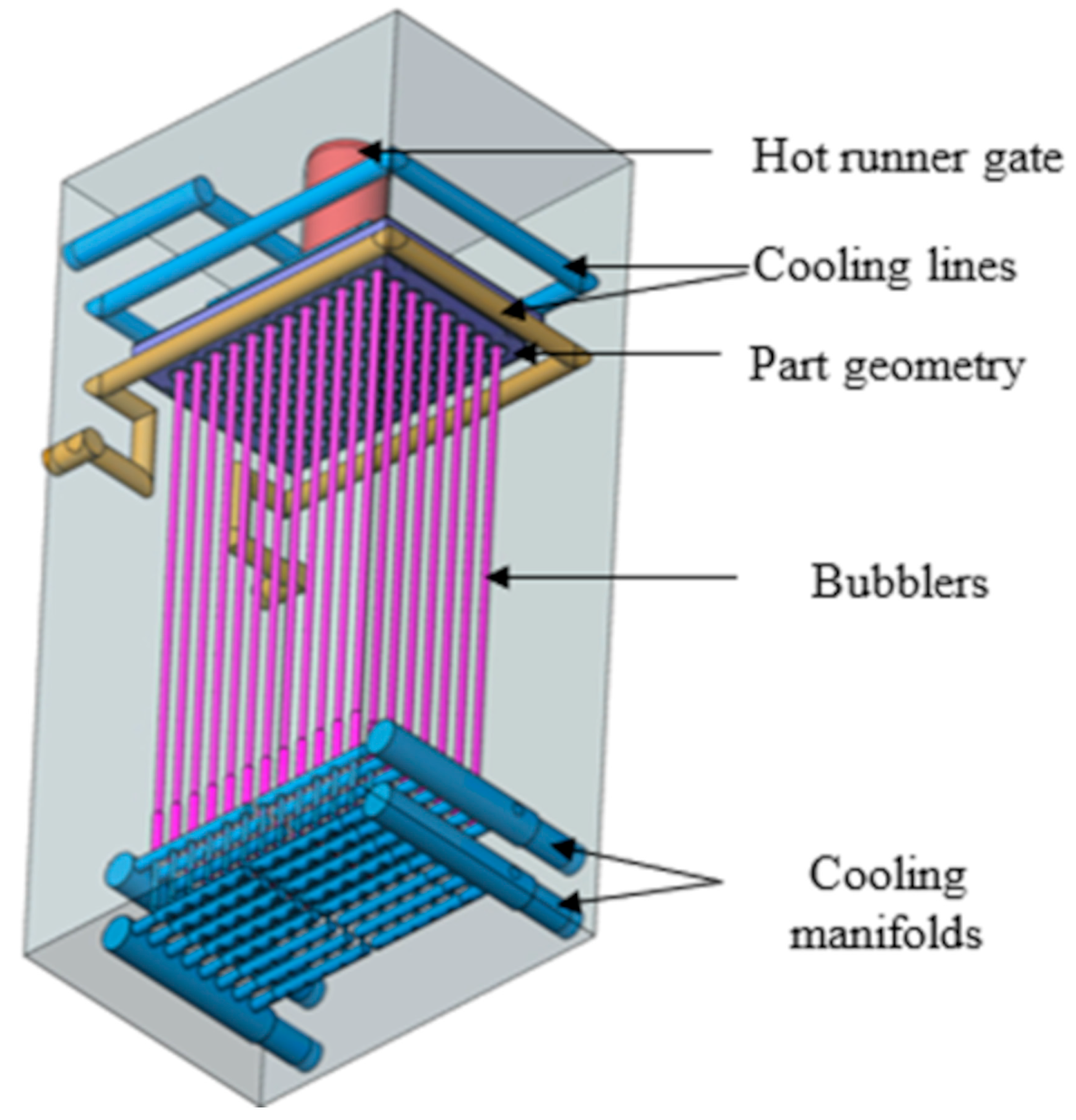
To avoid conflicts with the ejection system, the bubblers extend significantly into the B-side of the mold, resulting in elongated cooling channels with high aspect ratios. In these small channels, flow and thermal gradients are more pronounced, increasing the possibility of limescale deposition [16]. Different numerical models were developed to study the effects of limescale deposition on cooling performance and part dimensional stability. Compared to previous studies, the focus was on isolating the effects of thermal insulation and flow restriction. All simulations were run using Autodesk Moldflow Insight 2023. For all models, a 3D tetrahedral mesh with a global edge length of 5 mm was used for the part geometry, with sufficient resolution to capture the cooling channels and local geometric features. Figure 1 illustrates the simplified block design isolated from the entire mold design for the study.

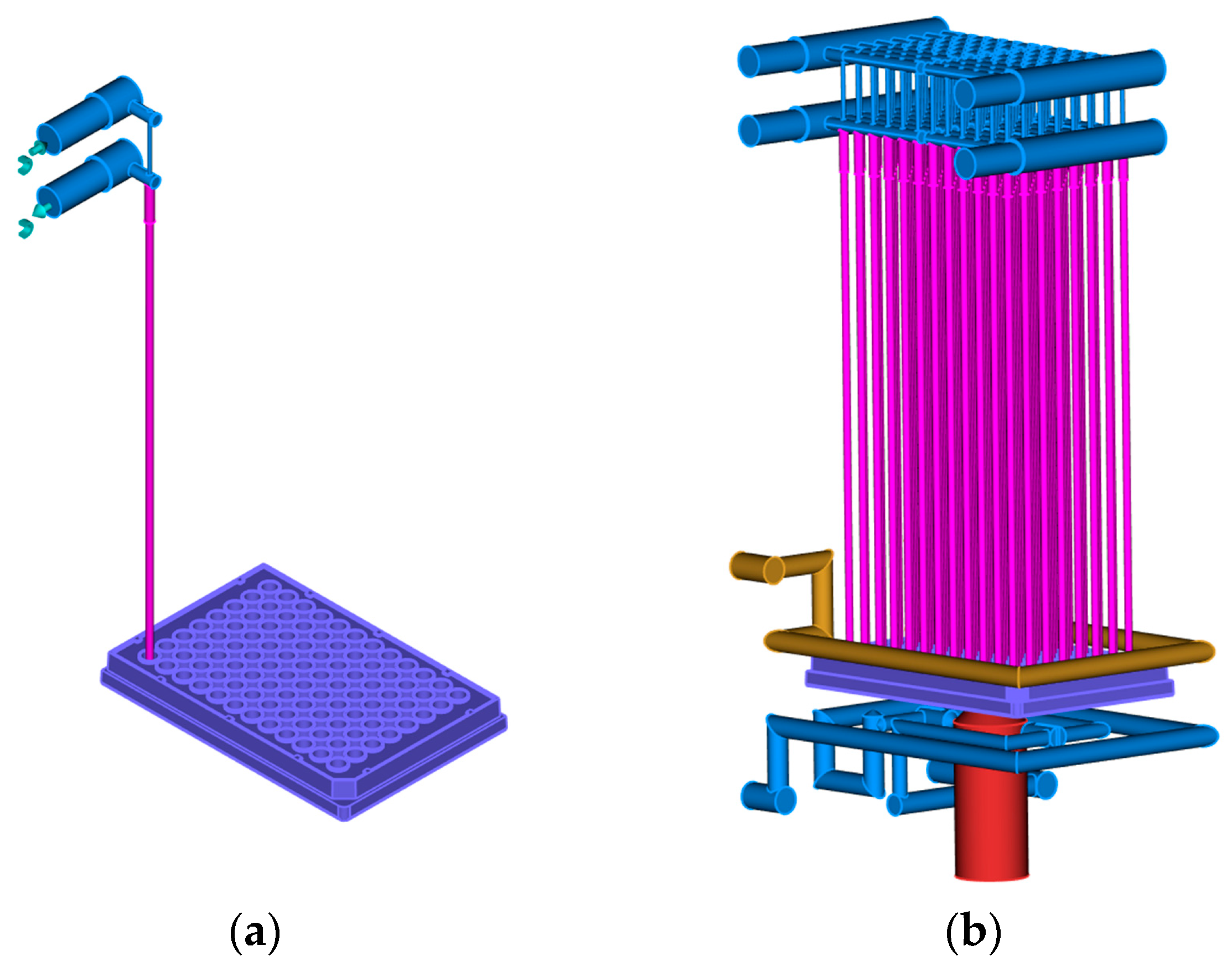
Considering the geometrical complexity of the mold, two different models were defined (see Figure 2 and

Table 1. Mesh density for the two models (all elements are tetrahedral).

Model	Number of Mesh Elements [Millions]			Analysis Type	Computational Time [Days]
	Part	Cooling Lines	Mold
Simplified	9.9	0.5	5.5	Cooling (FEM)	1
Full-scale	9.9	7.5	10	Cool (FEM), Fill, Pack, Warp	5

):

• Simplified Model: modeling of a single bubbler to isolate the effects of limescale on heat transfer and flow restriction. The other bubblers and cooling lines are disregarded.
• Full-Scale Model: modeling of the whole 96-bubbler cooling system to calculate mold temperature around the entire part.

For both models, the same parameters and processing conditions were used to ensure consistency, as shown in

Table 2. Process parameters and settings for the two simulations.

Process Parameters	Inputs
Material	Polystyrene
Melt temperature [°C]	200
Mold material	P20
Coolant	Water
Coolant pressure [kPa]	250
Mold temperature [°C]	45
Ejection temperature [°C]	108

.

The cooling analysis was performed using the Cool (FEM) module in Autodesk Moldflow Insight, which employs a finite-element formulation to model the coupled thermal-fluid behavior in the cooling system. Coolant flow was defined using prescribed inlet pressure conditions (Table 2), while outlet conditions were determined internally by the solver based on system flow resistance. The coolant was modeled as water, and the analysis was inherently transient, capturing the time-dependent heat transfer between the polymer, mold, and coolant throughout the molding cycle. The coolant temperature was defined through the thermal boundary conditions of the Cool (FEM) analysis and handled within the coupled solution.

Wall roughness was not explicitly specified and was therefore accounted for through the default assumptions embedded in the empirical correlations used by the Moldflow solver. Coolant flow in the channels was modeled using engineering correlations based on internal pipe flow theory. In this framework, the Reynolds number characterizes flow conditions and governs both hydraulic losses and convective heat transfer. Frictional losses were evaluated using empirical correlations (e.g., Swamee–Jain) consistent with the Darcy–Weisbach formulation, which depends on Reynolds number and channel roughness [20]. Similarly, convective heat transfer at the coolant-mold interface was determined through Reynolds–Nusselt-based correlations for internal flows [21]. Accordingly, turbulence effects were not defined through conventional turbulence models (e.g., k-ε or k-ω) but were implicitly represented through Reynolds-number-dependent correlations.

The numerical solution was obtained using the standard solver settings available within the Cool (FEM) analysis. Although a global edge length of 5 mm was assigned to the mold domain, the limescale layer was meshed as a separate component, resulting in locally refined elements with sizes significantly smaller than the global setting, consistent with the geometric scale of the deposit layer. This automatic local refinement ensured adequate geometric representation of the annular gap and reduced the flow area associated with limescale deposition. Although a formal mesh sensitivity study was not conducted, the selected mesh yielded stable, consistent trends in key output variables (e.g., coolant flow rate, Reynolds number, and cooling time) across the investigated cases. Therefore, the results are interpreted primarily within a comparative, trend-based framework rather than as absolute quantitative predictions. The observed trends are consistent with classical scaling relationships for internal flows, supporting the physical validity of the numerical results.

This numerical framework is based on well-established heat transfer and internal flow correlations implemented in the Moldflow Cool (FEM) solver. The trends observed in the present simulations, such as the dependence of cooling performance on flow rate, Reynolds number, and thermal resistance, are consistent with the established literature [14,15], supporting the physical validity of the model. Accordingly, the framework provides a consistent basis for comparative analysis of limescale effects under controlled conditions.

2.2. Limescale Definition and Modeling

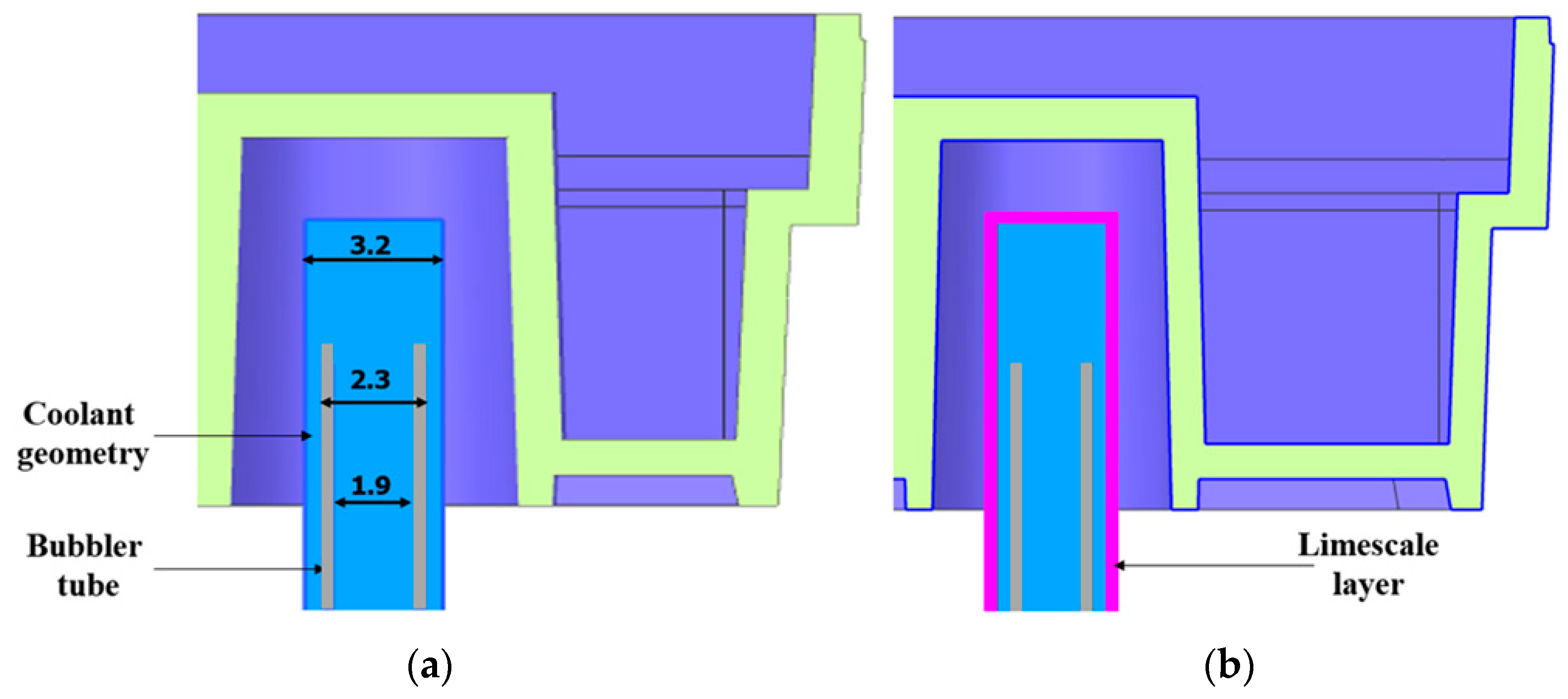
To analyze its effects, limescale deposition was modeled on the inner surface of the bubblers, as shown in Figure 3. The deposit was represented as a uniform annular layer (0.1 mm thickness) along the channel length, implemented in the CAD model and imported into Moldflow as a solid 3D mesh. This representation enables both flow restriction and the assignment of specific thermal properties.

Thermal properties were assigned based on the experimental measurements reported by Zink et al. [17], who characterized six limescale samples collected from injection mold cooling circuits, obtaining an average thermal conductivity (λ) of 1.37 ± 0.43 W/(m·K) over a range of 0.56–1.74 W/(m·K) depending on sample composition and an average specific heat capacity (cp) of 800 J/(kg·K). Although this range indicates significant variability in limescale composition, the selected average value is representative of compacted deposits typically found in mold cooling channels. Variations within this range are expected to influence the magnitude of heat transfer, but not the overall trends discussed in this work. Accordingly, the results are interpreted in terms of relative trends rather than as absolute predictions of limescale behavior.

The limescale layer was modeled in direct contact with the mold surface to affect the coolant/mold heat-transfer interface. A uniform thickness was assumed as a controlled simplification in the modeling. Although actual limescale deposition is typically non-uniform and influenced by local flow and thermal conditions, this assumption enables a consistent evaluation of its coupled thermal and hydraulic effects. In models that include limescale, an ideal interface conductance (i.e., 30,000 W/m²·K) was assumed at the mold/limescale interface due to the lack of reliable experimental data for fouling layers under these conditions. While actual limescale layers may introduce additional interfacial resistance due to imperfect contact, roughness, and potential interfacial voids, this would increase the overall thermal resistance associated with the deposit. Therefore, the present assumption may lead to a conservative estimation of the thermal contribution of limescale. However, the results indicate that, under the investigated conditions, performance degradation in slender channels is strongly influenced by flow restriction effects associated with reductions in hydraulic diameter. Accordingly, while the thermal effect may be underestimated in absolute terms, the comparative trends observed in this study are not expected to change under the investigated conditions.

Within the simplified model introduced in Section 2.1, two limescale modeling approaches were defined to isolate the relative contributions of thermal insulation and hydraulic restriction. In the first approach, limescale was introduced as a low-conductivity layer without modifying the coolant flow section, allowing the thermal resistance effect to be evaluated independently. In the second approach, the same limescale layer was modeled together with a reduced coolant flow area, thereby accounting for both thermal resistance and flow restriction. This distinction enables the decoupling of both mechanisms and clarifies their respective roles in cooling degradation. In particular, while variations in limescale thermal conductivity affect the local heat-transfer magnitude, the reduction in hydraulic diameter directly alters coolant flow rate and convective heat-transfer conditions, which can become a dominant factor governing cooling performance under confined geometries such as bubbler channels.

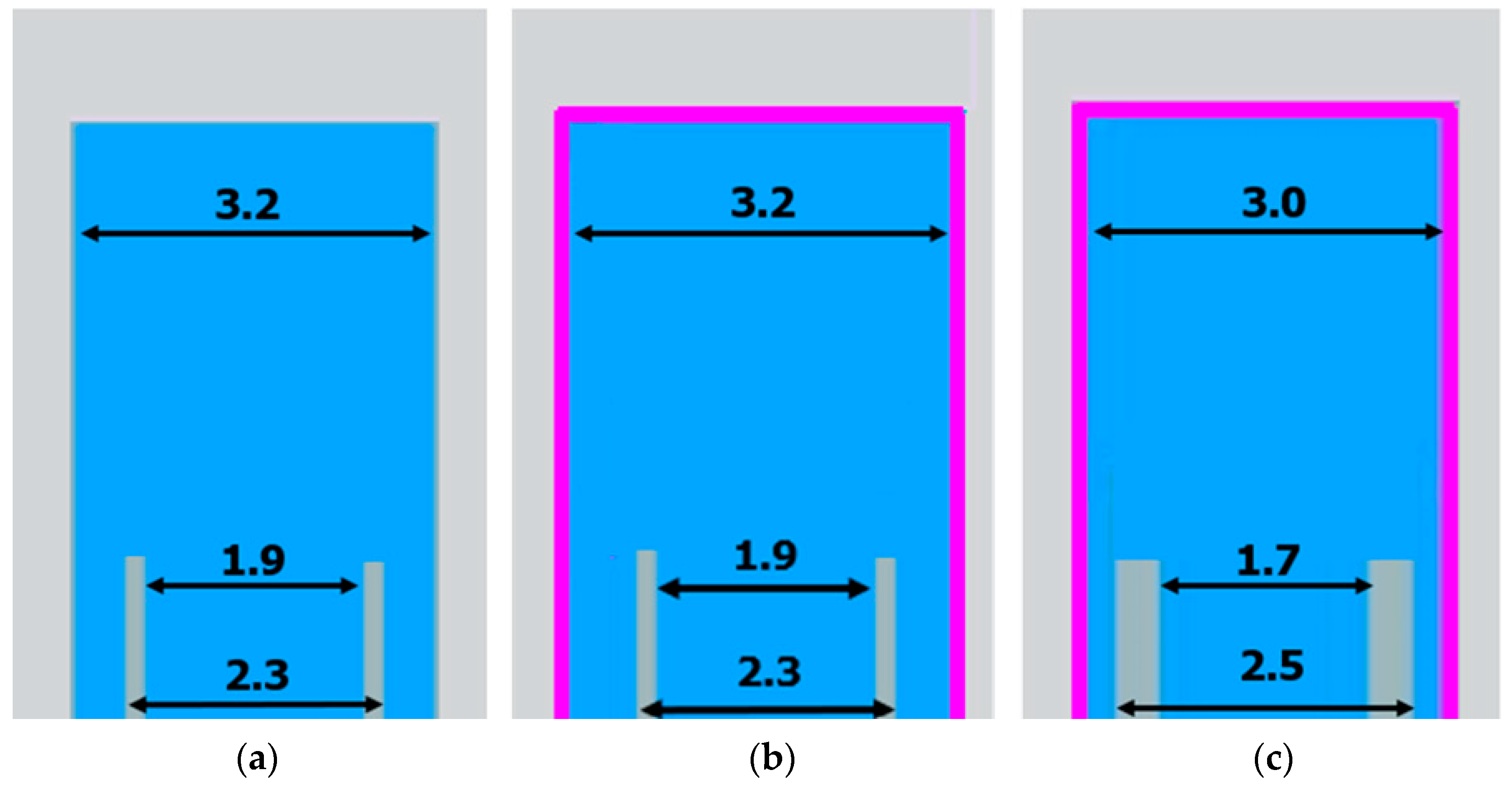
Figure 4 provides an overview of these two limescale modeling approaches and their respective geometrical definitions. Specifically, Figure 4a shows the model without limescale, corresponding to ideal conditions. Figure 4b illustrates a model with a low-thermal-conductivity limescale layer but no effect on the coolant flow sections (i.e., the dimensions are the same as those of the ideal model). Figure 4c shows the model with a low-thermal-conductivity limescale layer and reduced coolant flow diameters (i.e., both inside and outside the bubbler tube). For all models, Cool (FEM) analyses were conducted to evaluate changes in coolant flow rate, the increase in coolant temperature from inlet to outlet, part temperature, and the time to reach ejection temperature. Considering the limitations of the single-bubbler model, the part results were analyzed locally around the bubbler, disregarding the effects on the remainder of the cavity.

After isolating and analyzing the effects of the two modeling approaches on limescale deposition, the deposit thickness was varied. Deposits of 0.05 mm and 0.15 mm were evaluated, corresponding to approximately 1.6% and 4.7% of the 3.2 mm diameter of the cooling channel, respectively. It should be noted that these values are significantly smaller than those reported by Zink et al. [22] (e.g., 0.25–2 mm, representing 3–25% of typical 5–8 mm cooling channel diameters), which focused on larger, more conventional cooling line diameters. The smaller relative thicknesses investigated here more accurately represent the conditions encountered in precision molds, where even minor deposits can significantly impact heat-transfer efficiency.

Although direct experimental validation was not performed in the present study, the modeling approach is based on correlations for internal flow and heat transfer, with pressure losses and convective heat transfer governed by Reynolds-number-dependent formulations consistent with classical approaches (e.g., the Darcy-Weisbach and Nusselt correlations). The observed trends, such as the sensitivity of flow rate and heat transfer to reductions in hydraulic diameter, are consistent with fundamental fluid mechanics and prior literature trends [14,15,19]. Therefore, the results are interpreted primarily as comparative, trend-based findings rather than as absolute quantitative predictions.

2.3. Simulation Studies

The numerical investigation of the effects of limescale on cooling performance focused on studying different coolant conditions and bubbler designs using the simplified model.

Table 3. Factors and level settings in the design of experiments.

Factors	Level 1	Level 2
Coolant Pressure [kPa]	50	250
Bubbler Length [%]	50	100
Limescale [mm]	0	0.1

reports the factors and levels used in the design of the experiment. The two-level DOE was used as a screening study to identify the primary effects of limescale, coolant pressure, and bubbler length on the thermal-fluid response of the system, rather than to establish a full parametric description of the design space. This approach enables the identification of dominant factors while maintaining computational feasibility for the complex full-scale model.

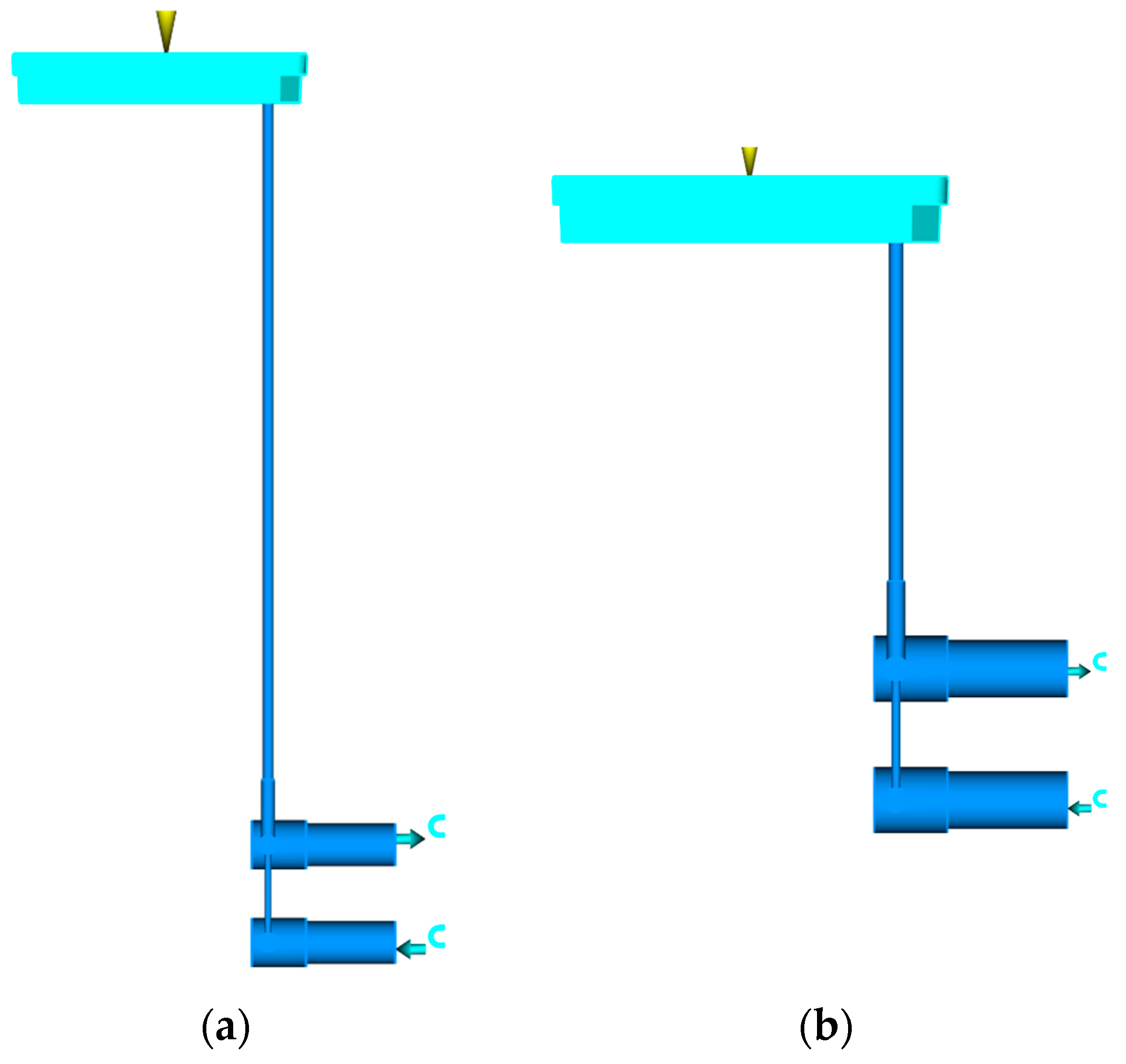
The coolant pressure was varied, as it is a critical parameter for controlling injection-molding cooling systems, with the selected levels defined to represent typical process adjustments (e.g., variations in coolant pressure and flow rate). The bubbler length in the mold base was shortened (cf. Figure 5) to evaluate the possibility of reducing the coolant flow path through mold base design optimization, representing feasible design modifications to the bubbler geometry. Finally, comparisons were made with and without limescale, modeled exclusively along the length of the bubblers, disregarding buildup in the cooling lines, to represent the presence of deposits commonly observed in injection-molding cooling systems. The results analysis focused on evaluating coolant flow turbulence (i.e., Reynolds number), coolant flow rate, and time to reach the ejection temperature. All simulations were conducted using the same boundary conditions and process parameters defined in Table 2. Additional simulations at intermediate and higher pressure levels were subsequently performed as a complementary sensitivity analysis to examine the influence of coolant pressure on thermal-fluid performance and to identify the onset of diminishing returns.

The full-scale model was developed to validate trends identified in the simplified model and to calculate the temperature distributions of the entire part and mold, ultimately enabling warpage calculations. The simplified model enabled a localized assessment of the effects of limescale thickness and flow restriction on thermal-fluid behavior within individual bubblers. These insights were subsequently transferred to the full-scale model to evaluate how localized mechanisms influence the global thermal response of the mold and the resulting part quality, including temperature distribution, shrinkage, and warpage. To achieve these goals, a complete analysis sequence (i.e., Cool (FEM), Fill, Pack, and Warp) was performed, enabling the study of limescale-induced thermal effects on cooling performance and part quality. Specifically, two models were evaluated: (1) the baseline design with 0.10 mm limescale buildup in the bubblers (i.e., worst-case scenario), and (2) an improved configuration incorporating the optimized bubbler length without limescale deposition (i.e., best-case scenario). The comparison enabled a quantitative assessment of how limescale affects cooling performance and how design modifications can mitigate adverse effects on part quality and dimensional stability.

3. Results and Discussion

3.1. Simplified Model

3.1.1. Approach to Limescale Modeling

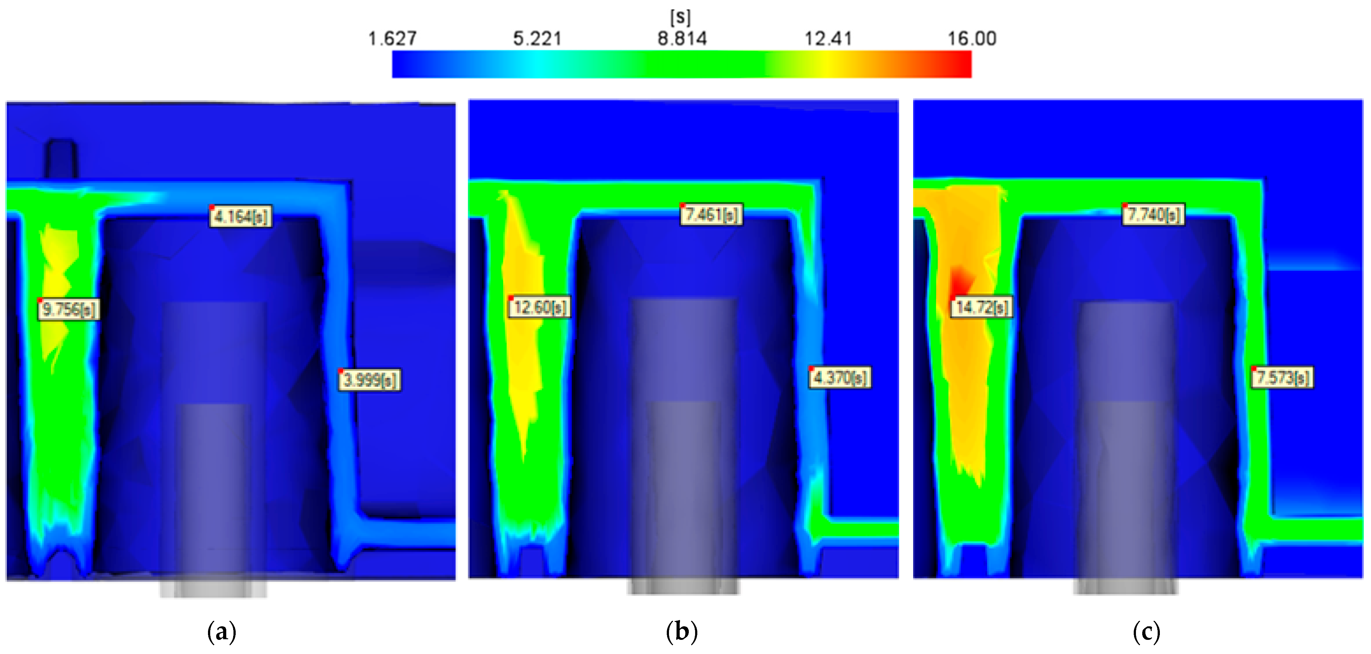
Figure 6 compares the time to reach the ejection temperature results for the models defined in Figure 4, simulated under constant coolant pressure (250 kPa). The same nodes around the bubbler were probed in all models, and the average time to reach the ejection temperature was calculated.

In the model with no scale (Figure 6a), the maximum ejection time around the bubbler was 9.8 s, which served as the baseline reference for subsequent comparisons. Introducing a 0.1 mm limescale layer, considering only its thermal resistance (Figure 6b), extended the time to ejection temperature by 29%. When both thermal resistance and flow restriction were included (Figure 6c), the increase reached 51%. These results demonstrate that the combined effects of flow restriction and low thermal conductivity have the most severe impact on cooling performance. The addition of a limescale layer reduces the effective cross-sectional area of the cooling channel, lowering coolant velocity and Reynolds number, and thereby weakening turbulence and heat transfer at the fluid–wall interface. These effects are particularly critical in the 3.2 mm bubbler studied here, where even thin deposits occupy a substantial fraction of the flow area. While Zink et al. [17] also reported the insulating effect of limescale in conventional channels, the slender annular geometry analyzed here is markedly more sensitive to partial blockage. This modeling approach was retained for subsequent analyses, as it provides a more realistic representation of the conditions that may occur during actual mold operation, where small deposits can trigger disproportionate cooling inefficiencies.

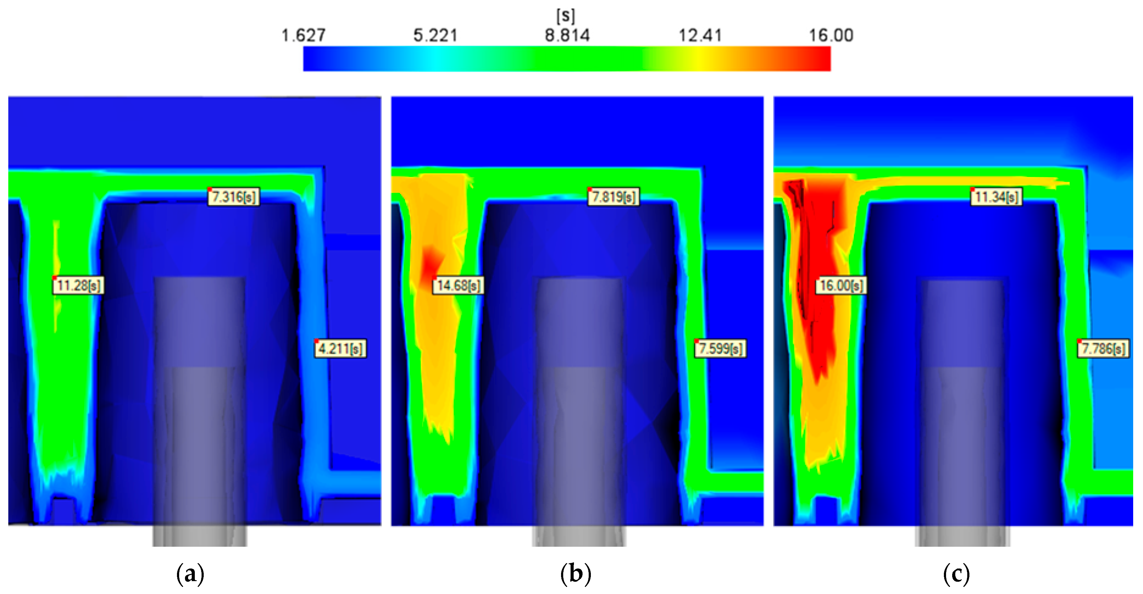
Figure 7 quantifies the effect of increasing the limescale thickness on the time to reach the ejection temperature under constant coolant pressure conditions. As the limescale thickness increased from 0.05 mm to 0.15 mm, the effective cross-sectional area of the cooling channel decreased, leading to a significant drop in the coolant velocity from 3.4 m/s to 1.4 m/s, resulting in a 64% increase in ejection time for the thickest layer compared to the no-limescale case (42% relative to the 0.05 mm deposit). This outcome is consistent with heat-transfer principles: the convective heat-transfer coefficient increases with flow velocity, as reflected in the Reynolds number (Re), which governs the flow regime and turbulence level. Under the constant-pressure condition, Re decreased sharply from approximately 4150 for the bubbler with no limescale (turbulent) to about 2380 for the 0.05 mm deposit (transitional) and to 750 and 425 for the 0.10 and 0.15 mm deposits, respectively. This progression reflects a transition from turbulent to transitional and ultimately laminar flow, which significantly reduces mixing at the fluid–wall interface and degrades convective heat transfer in this confined annular geometry. The Reynolds number was calculated using the annular section’s hydraulic diameter and the average coolant velocity. The latter was obtained from the simulated velocity field at the outlet section of the annular gap, where the coolant is in direct contact with the mold wall. The local heat-transfer behavior follows the expected positive correlation between the Nusselt number and the Reynolds number in the transitional-to-turbulent regime; therefore, the observed reduction in Re directly lowers the convective heat-transfer coefficient (h), diminishing the system’s ability to remove heat effectively. The reduction in hydraulic diameter increases the overall flow resistance, which, under constant inlet pressure, lowers the mass flow rate and coolant velocity toward the end of the bubbler. This behavior is consistent with classical pipe-flow theory, in which pressure losses increase sharply as the hydraulic diameter decreases. Such sensitivity is particularly critical in narrow cooling channels, where even small deposits can severely impair flow and thermal performance [4,14].

Notably, the 0.15 mm layer corresponds to 4.7% of the 3.2 mm channel diameter. However, in the annular section of the bubblers, this same thickness reduces the radial clearance between the inner and outer walls from 0.45 mm to 0.15 mm, representing a 67% decrease in gap height. This geometric change makes hydraulic resistance the dominant limitation, even when the thermal properties remain unchanged. Therefore, a 0.10 mm layer was selected for further analysis because it provided a measurable increase in ejection time, confirming the combined impact of thermal and flow restrictions while maintaining sufficient coolant velocity to ensure through-flow along the entire length of the bubbler.

3.1.2. Effects of Limescale on Coolant Flow and Localized Heat Transfer

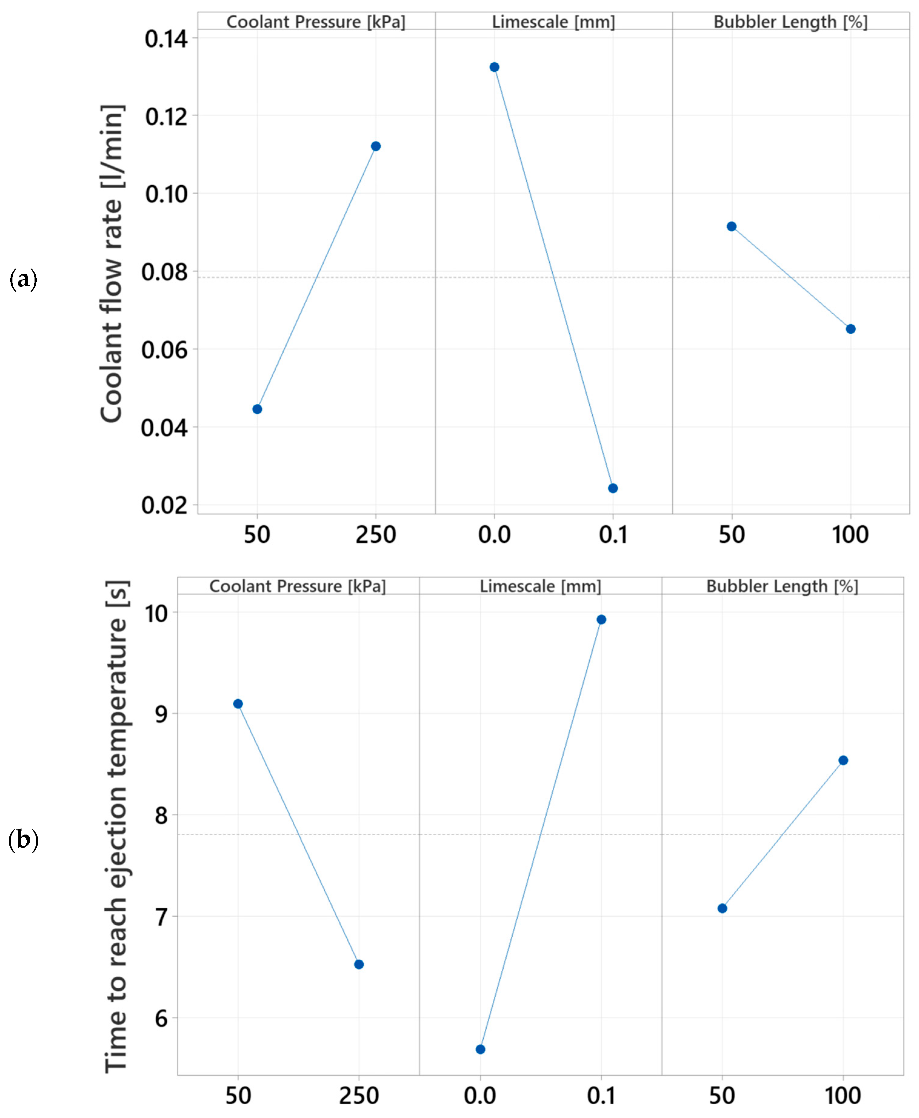
The results of the simulation DOE (cf. Table 3) are presented in Figure 8. The main-effect plots are used to evaluate the impact of limescale on cooling performance under various coolant conditions and bubbler lengths.

Figure 8a shows that the formation of a 0.1 mm layer of limescale on the surface of the bubblers results in a 71% reduction in the coolant flow rate and a corresponding 67% decrease in the calculated Reynolds number. As discussed above, this reduction in Reynolds number weakens turbulence and convective heat transfer, as higher Reynolds numbers promote fluid mixing and heat-transfer efficiency [14]. This behavior results from flow obstruction, as the deposit reduces the effective cross-sectional area under constant inlet pressure. Increasing coolant pressure and reducing bubbler length partially mitigate this effect by improving flow delivery and reducing frictional pressure losses along the coolant path.

To provide a more explicit link between flow conditions and convective heat-transfer performance, the Nusselt number and convective heat-transfer coefficient were estimated in a post-processing step from the Reynolds numbers characterizing each case, using classical correlations for internal flow [21]. A Prandtl number of Pr = 3.9 and thermal conductivity of water k = 0.64 W/m·K at the operating coolant temperature (45 °C) were assumed, and the hydraulic diameter of the annular channel was used as the characteristic length. The Gnielinski correlation was applied for turbulent and transitional conditions, while a constant Nusselt number (Nu = 3.66) was assumed for laminar flow [21]. For the baseline case (Re = 4158), Nu = 26.5 and h ≈ 18,760 W/m²K. With a 0.05 mm deposit (Re = 2380), Nu decreases to 13.1 and h to approximately 9270 W/m²K, a 51% reduction relative to the baseline. For deposits of 0.10 mm and 0.15 mm, the flow is laminar, and Nu converges to 3.66, yielding h ≈ 2590 W/m²K, an 86% reduction relative to the clean channel. Notably, both laminar cases yield identical values, as the Nusselt number becomes independent of the Reynolds number under fully developed laminar flow. While these values should be interpreted as engineering estimates given the annular geometry and transitional flow conditions, they consistently support the conclusion that hydraulic restriction is the dominant performance-limiting mechanism in slender cooling channels.

These thermal-fluid effects directly translate into improved cooling performance, as shown in Figure 8b. The factors influencing flow are directly reflected in the time required for the part to reach ejection temperature. The addition of limescale increased cooling time by nearly 50%, a result consistent with the drop in flow efficiency. Conversely, higher coolant pressure and shorter bubblers improved cooling performance, confirming that thermal transport losses induced by limescale can be partially recovered through design and process adjustments.

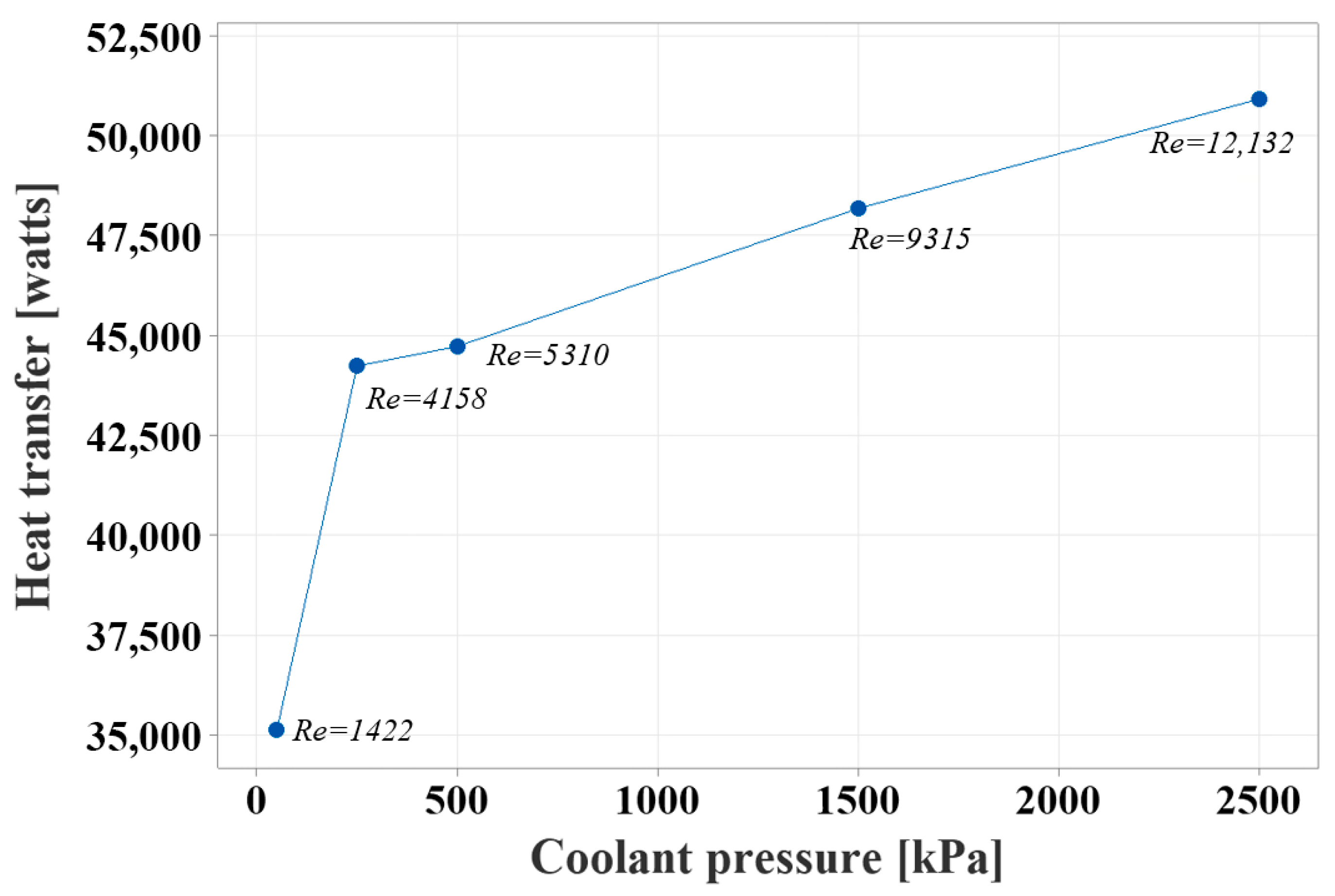
The effect of coolant pressure was evaluated by running simulations with inlet pressures of 50, 250, 500, 1500, and 2500 kPa. The heat removed by the single bubbler was calculated from the coolant mass flow rate, specific heat, and the temperature difference between the inlet and outlet. Figure 9 shows that heat transfer increases with coolant pressure, a result of the higher mass flow rate and corresponding rise in Reynolds number, which enhances convective turbulence and surface heat-transfer efficiency.

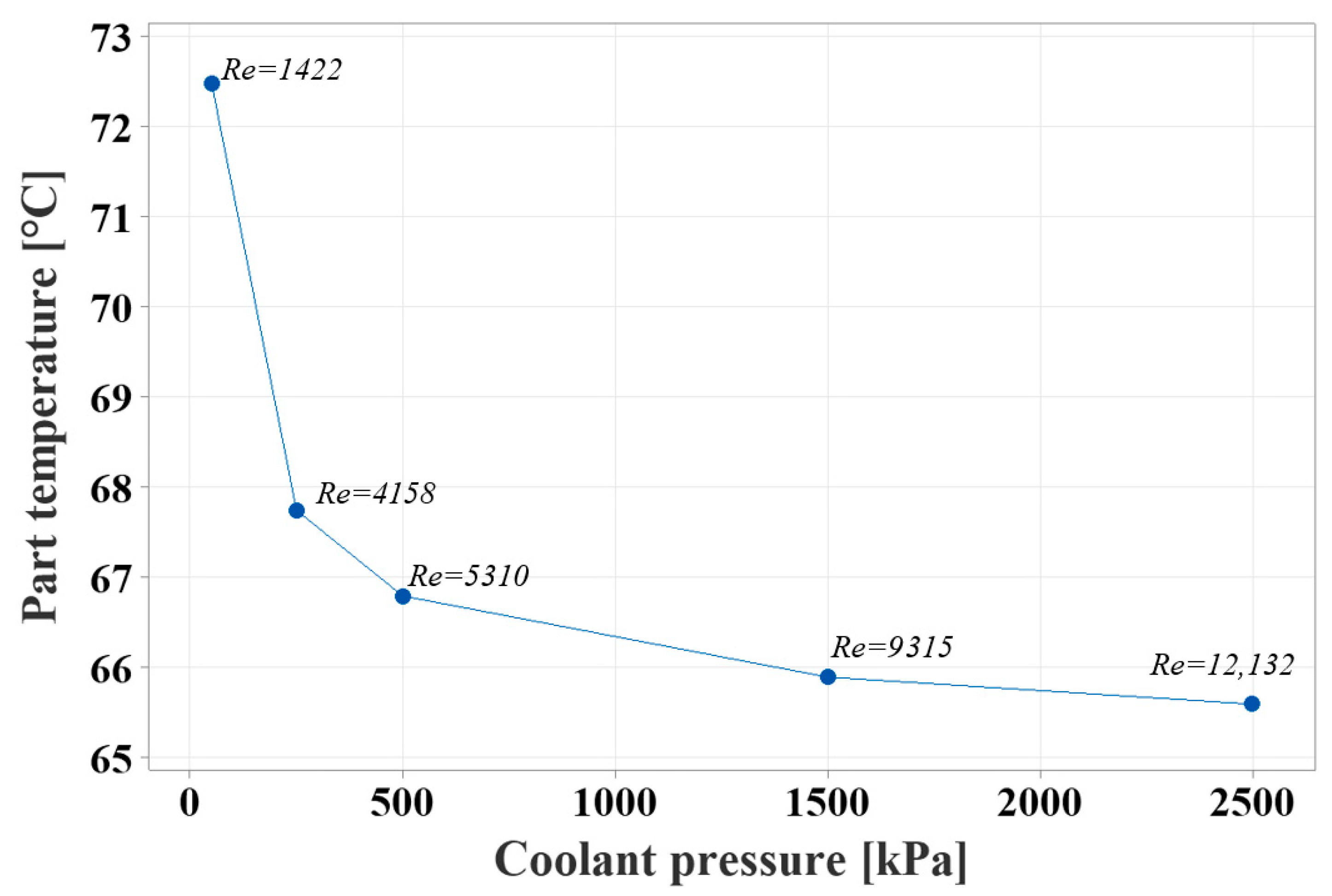
Figure 10 confirms the existence of a plateau in the performance. As coolant pressure increases, the part temperature continues decreasing, but the rate of improvement diminishes beyond 1500 kPa. At this stage, the dominant thermal resistance shifts from the coolant-side convection to the conductive path through the steel between the channel and cavity surface. As described by Rashid et al., the total thermal resistance in the system results from two main contributions acting in series: one from coolant-side convection and another from the steel bulk between the cooling channel and the cavity surface. As coolant-side heat transfer improves (due to turbulence), the steel’s resistance eventually becomes dominant, limiting further gains [4].

Similar trends have been observed in the literature; for instance, Gao et al. showed that beyond a Reynolds number of approximately 20,000, cooling performance does not significantly improve but substantially increases pressure drop and pumping requirements [15]. Although their study focused on a different mold geometry and cooling design, naturally yielding higher critical Re values, the underlying principle remains relevant: for process optimization, once internal turbulence is sufficiently developed to break down the thermal boundary layer, further increases in flow are governed by the interface resistance, primarily driven by material contact, surface conditions, and limescale deposits.

The simulations in the present study enable a direct assessment of this thermal–flow trade-off, identifying an application-specific lower optimal operating point. The emergence of a temperature plateau beyond 1500 kPa (see Figure 10) in this narrow-channel bubbler suggests that a similar diminishing behavior can occur at significantly lower Re values (Re < 4500), depending on the system’s geometry, materials, and cooling configuration. This highlights the importance of application-specific evaluations to avoid overdesign.

3.2. Full-Scale Model

3.2.1. Temperature Results

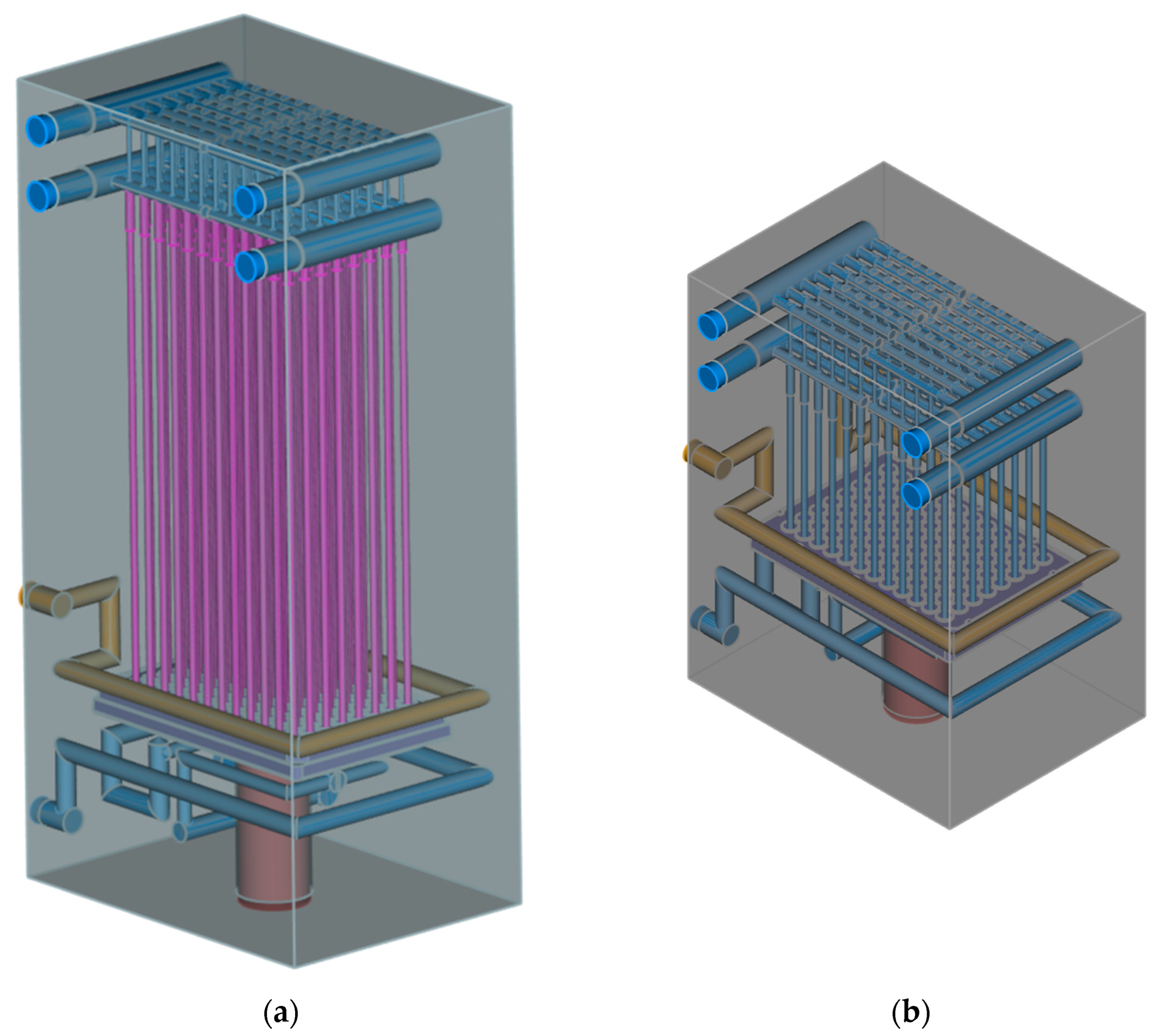
The impact of limescale on the complete 96-bubbler part was evaluated using the full-scale model to obtain part temperature and dimensional results. Two representative cases for comparison were defined, as shown in Figure 11. A worst-case design model (Figure 11a) was defined using the original configuration with 0.1 mm of limescale buildup and full-length bubblers. A best-case design model (Figure 11b) was modified to omit limescale and to reduce the bubbler extension.

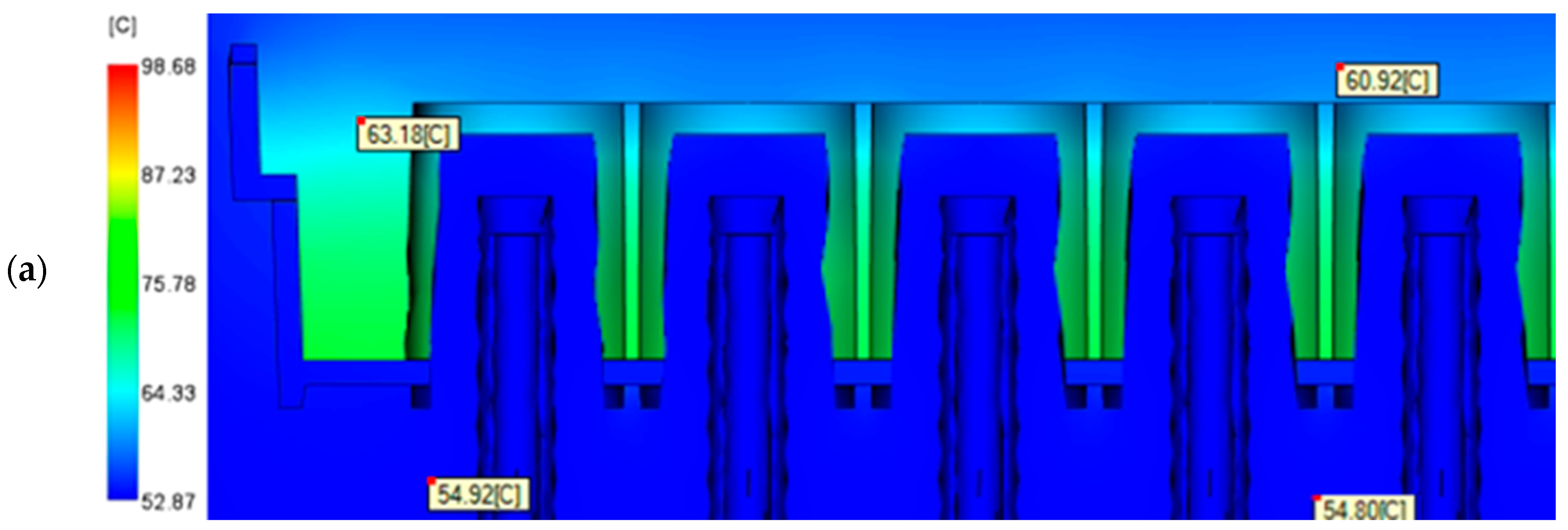
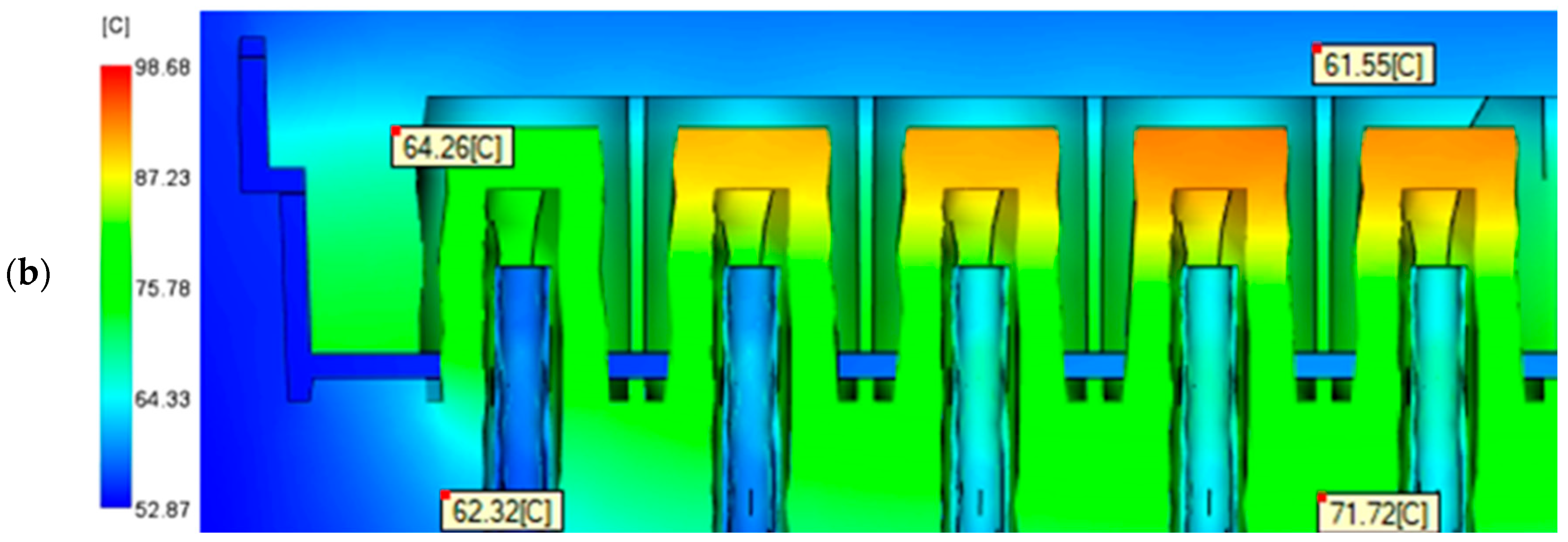
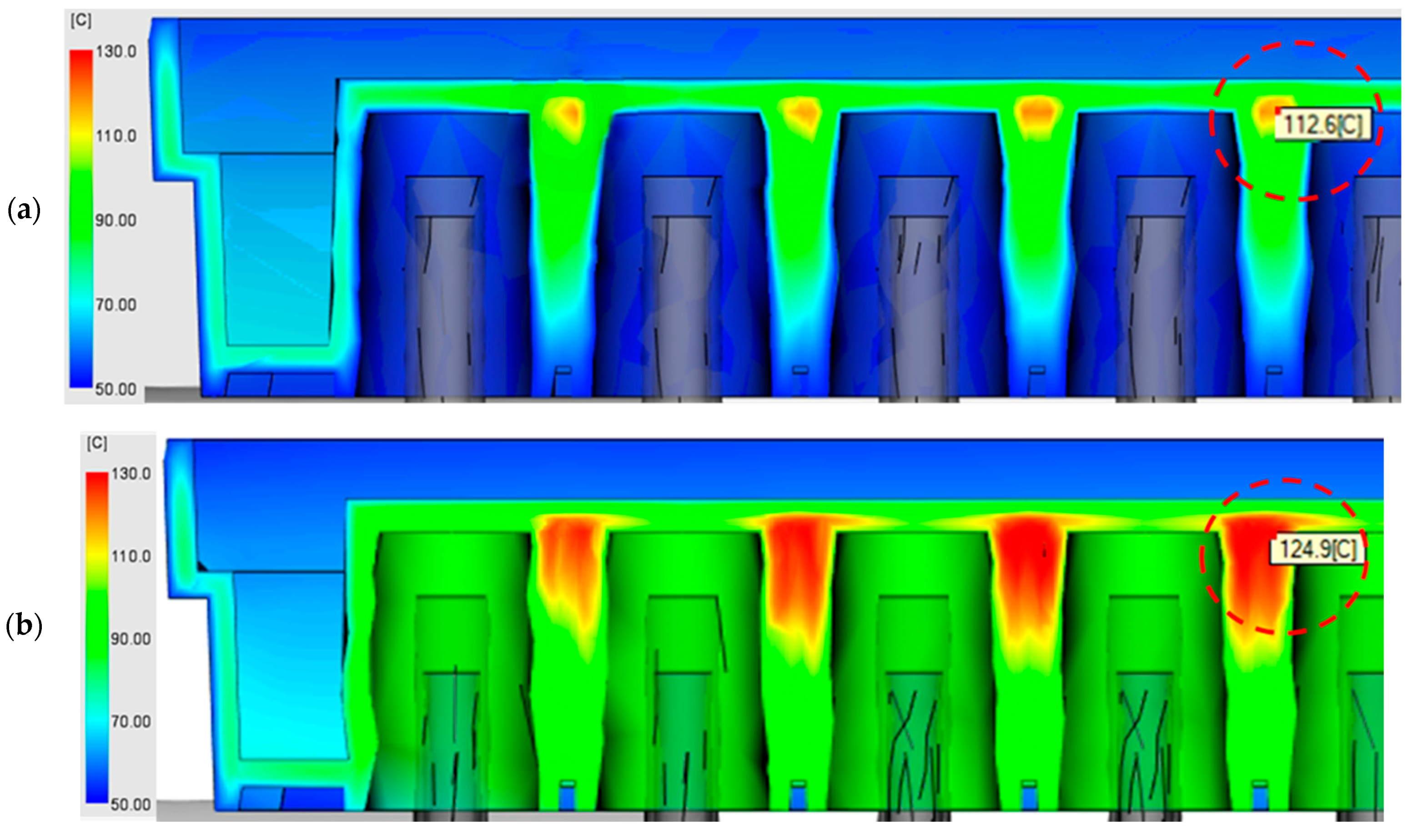
Figure 12 compares the mold temperature distribution for the two design approaches. For this analysis, a transverse cross-section was taken through the part at the injection location (hot runner tip). Due to the geometric symmetry of the part, only one side of the section is shown and evaluated, as the temperature distribution on the opposite side would be identical. The average mold temperature was calculated as the arithmetic mean of all nodal temperatures within the steel region of the mold cross-section shown in Figure 12. The resulting difference indicated that the worst-case design exhibited approximately 11% higher temperatures, consistent with the mechanisms identified in the simplified model. The presence of limescale increases interfacial thermal resistance while simultaneously restricting flow, thereby reducing heat removal capacity. Most of this temperature difference originates on the B-side of the mold, where reduced coolant delivery and a longer flow path amplify the thermal imbalance. These effects are compounded by the longer coolant path in full-length bubblers, where frictional pressure losses reduce flow delivery toward the far end of the channel, resulting in a hotter mold.

These mold temperature differences directly translate into the part temperature distribution. Figure 13 illustrates the part temperature at 7.71 s for the best- and worst-case designs. In both designs, the highest temperatures are at the center of the well plate, beneath the hot runner tip, as highlighted by the dashed circles. However, when evaluating how effectively each design approach removes heat from the part, significant differences become apparent. The worst-case design shows more diffuse high-temperature regions, indicating less efficient heat extraction than the best-case design. In contrast, the best-case design, with optimized cooling and no limescale, limits the spread of these hot zones, reflecting improved local heat removal capacity. The reduction in cooling performance in the worst-case design increases the time required for the part to reach the ejection temperature. At the hottest region of the part, the ejection time was 10.34 s, compared to 8.63 s for the best-case design, representing a 17% increase.

3.2.2. Shrinkage and Warpage Results

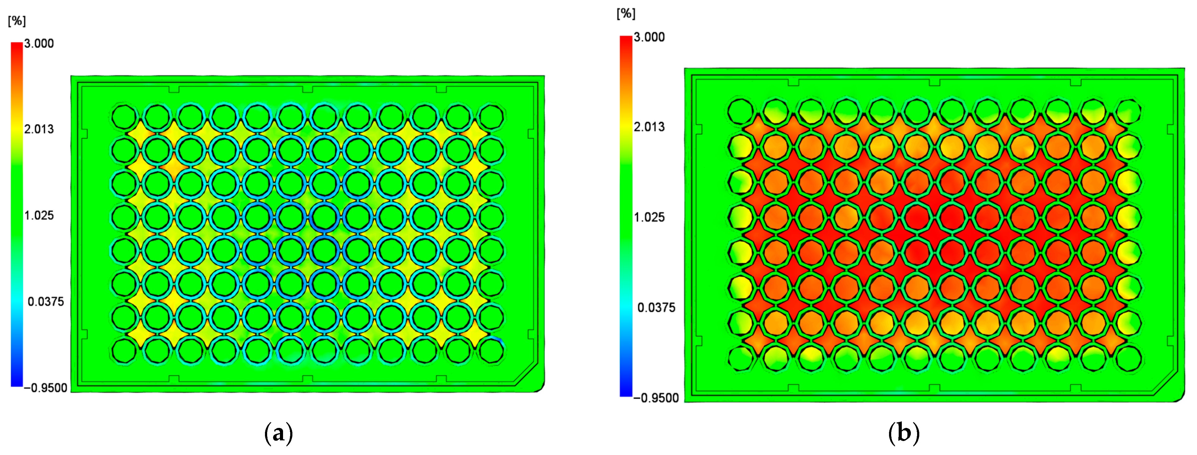
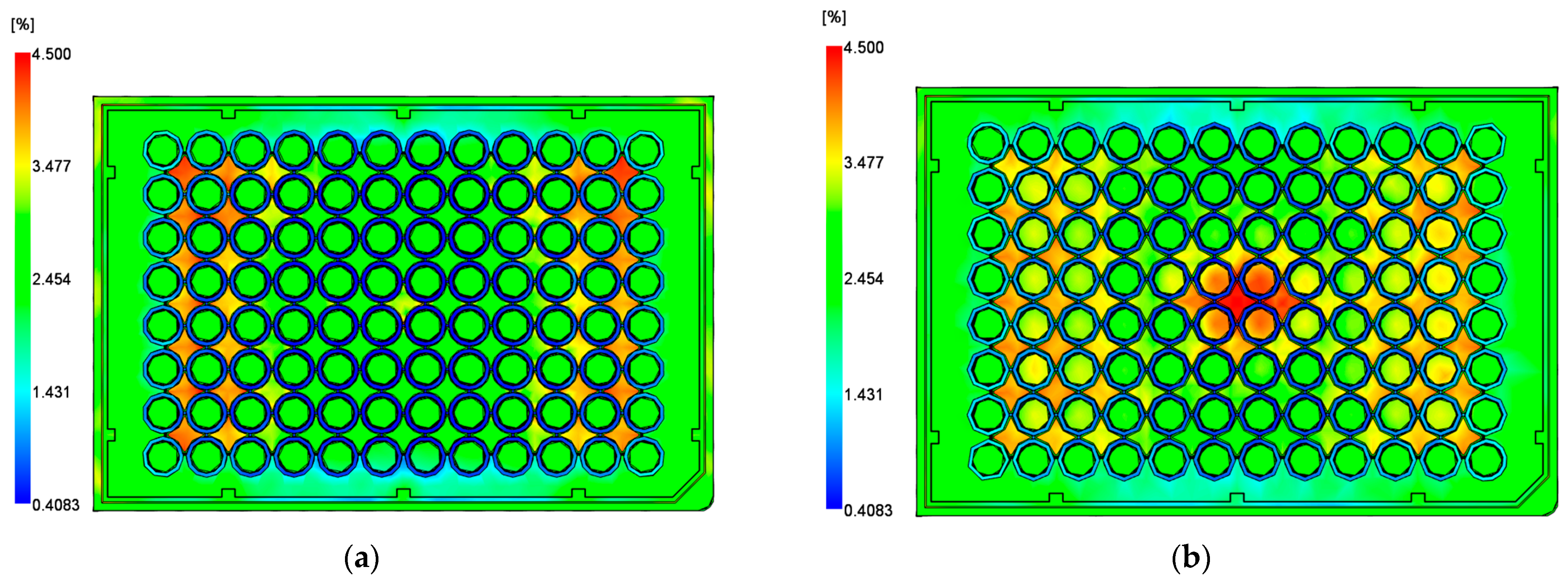
Figure 14 illustrates the shrinkage of the surface elements of the part. The same color scale was used in both cases to enable direct visual comparison. According to the mold temperature results, the best-case design exhibited a more uniform mold surface temperature, leading to more uniform surface shrinkage. In contrast, the worst-case design exhibited uneven shrinkage, with higher values concentrated in the center and lower values near the edges, highlighting the impact of cooling design and buildup on maintaining a uniform mold temperature and, consequently, on the surface shrinkage of the part.

When analyzing the average volumetric shrinkage across the part thickness in Figure 15, the worst-case design shows slightly lower shrinkage values. This behavior may be associated with the longer time allowed for the material to pack during cooling, which can enhance packing within the cavity and help maintain lower shrinkage across the part thickness. These results suggest that optimizing packing parameters to achieve the best-case design could result in comparable shrinkage performance while maintaining shorter cycle times.

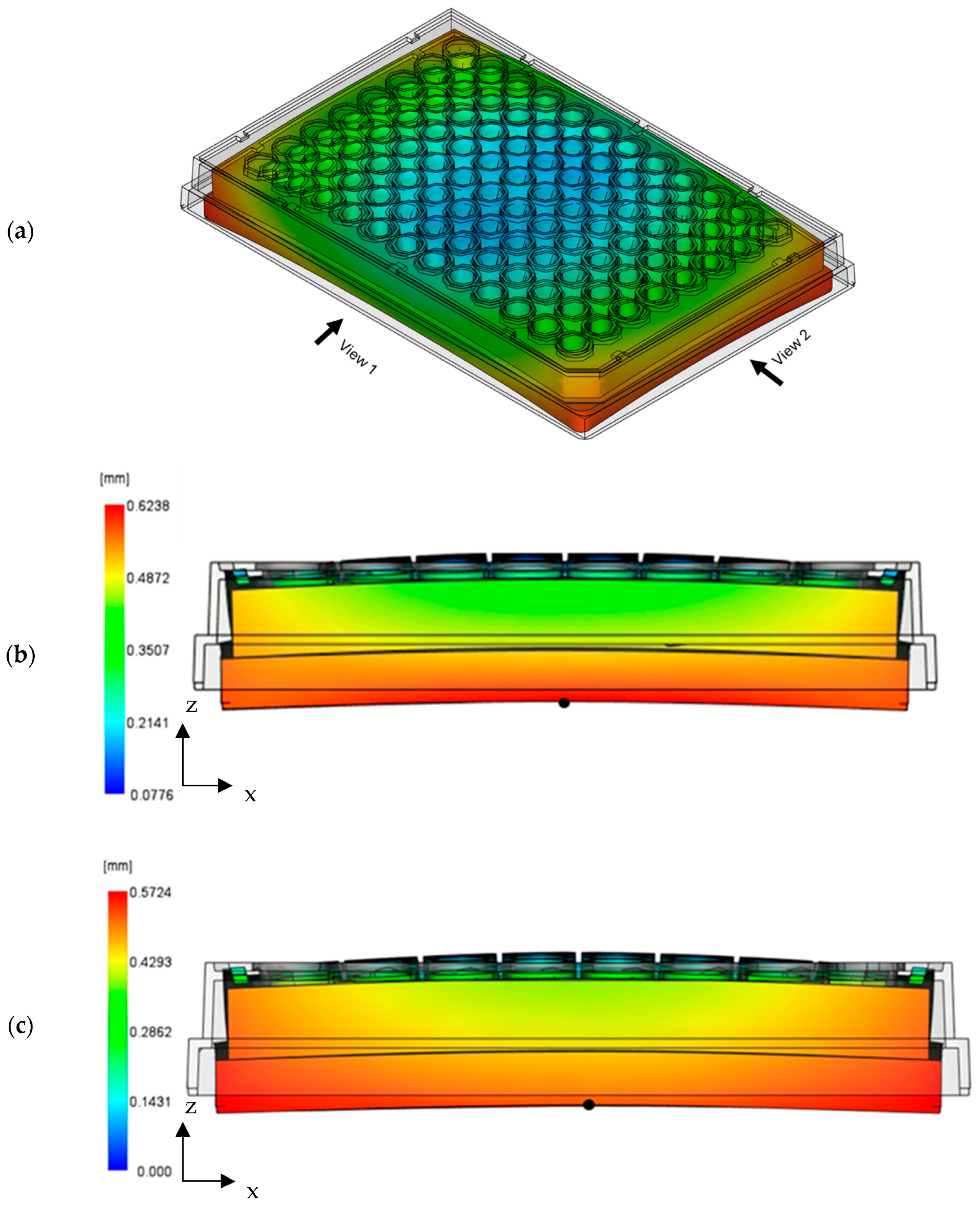
Figure 16 illustrates the part-deflection results for the best-case and worst-case configurations, explicitly examining deflection along the shorter edge (view 2). Warpage in injection-molded parts generally originates from internal stresses developed during cooling, driven by differential shrinkage through the thickness and across the geometry. These stresses are strongly influenced by the uniformity of heat removal, which is determined by the cooling system’s performance.

Table 4. Part warpage comparison between the two case studies.

Measurements	Best-Case Design	Worst-Case Design
Z deflection [mm]	0.09	0.09
ΔX [mm]	0.65	0.63
Shrinkage [%]	0.76	0.74

summarizes the warpage metrics for both cases. ΔX represents the dimensional change between the mold cavity length (measured end-to-end) and the corresponding post-molding dimension of the part. At the same time, Z-deflection quantifies the vertical displacement of the edge’s central point. For these measurements, one end of the part was anchored in the simulation as a reference point, ensuring consistent comparisons across cases.

The results show similar overall warpage magnitudes for both cases. The slightly lower ΔX in the worst-case design is consistent with the shrinkage trends discussed previously, where longer cooling times may promote more effective material packing within the cavity, thereby mitigating shrinkage differences. This interpretation aligns with prior studies showing that increased packing pressure or time can reduce differential shrinkage and the resulting warpage [23,24].

While both design cases exhibited similar warpage magnitudes, the best-case configuration offers potential for further improvement through process optimization. The literature shows that moderate increases in packing pressure can significantly reduce differential shrinkage and associated warpage without substantially increasing cycle time [25]. Based on these findings, the packing pressure in the best-case design was increased by 15%.

Table 5. Comparison of part warpage between the best-case design with the original parameters and with the increase in pack pressure.

Measurements	Best-Case Design Original Parameters	Best-Case Design Increased Pack Pressure
Z deflection [mm]	0.09	0.09
ΔX [mm]	0.65	0.61
Shrinkage [%]	0.76	0.72

compares part deflection in the x and z directions for the original best-case parameters and the best-case design with the increased packing pressure.

The results confirm that this adjustment effectively maintained low part deflection, which may be associated with more effective material packing during the holding phase, helping to offset shrinkage and associated warpage. This improvement was achieved without extending the cooling phase, thereby preserving the shorter cycle time.

4. Conclusions

This study presented a combined thermal-fluid modeling framework to quantify the impact of limescale on the cooling performance of high-aspect-ratio channels used in slender cores. The simulation results indicate that even small limescale deposits can significantly reduce cooling efficiency in these narrow geometries, with flow restriction emerging as a key mechanism influencing performance degradation under the investigated conditions. The key findings from the simplified and full-scale modeling approaches are summarized below.

The numerical study demonstrated that, in narrow bubbler channels, limescale effects are more strongly influenced by hydraulic restriction than by thermal insulation, even for small deposit thicknesses. This reduction in flow capacity directly limits convective heat removal, leading to substantial cooling penalties. In the simplified model, this resulted in up to an 85% increase in ejection time under the investigated conditions for the worst-case limescale thickness.

The proposed modeling framework also proved effective as a comparative design and optimization tool, showing that limescale in slender channels should not be treated solely as a thermal resistance but as a coupled thermal–hydraulic effect. This distinction is critical for engineering practice, as cooling performance becomes highly sensitive to flow degradation in slender geometries. Based on these insights, two complementary mitigation strategies were identified:

• Design Optimization: Reducing the overall pressure drop in the bubblers (i.e., minimizing the bubbler length) proved an effective strategy to improve cooling performance and counteract frictional losses, thereby enhancing coolant flow and heat-transfer efficiency.
• Process Optimization: The simulation methodology enabled the identification of an optimal operational pressure (up to 1500 kPa), effectively mitigating flow impairment caused by limescale and extending channel lengths. This helps avoid energy inefficiencies associated with overdesign, as cooling performance plateaus beyond this pressure threshold (Re < 4500). These pressure levels were investigated to evaluate how changes in coolant flow conditions may help counteract the adverse effects of limescale formation and to identify the onset of diminishing returns in cooling performance. From an engineering perspective, these results suggest the importance of identifying an application-specific thermal–flow trade-off rather than relying on a general limit.

The comprehensive analysis using the full-scale model further supports these findings, revealing that the worst-case design (limescale and extended bubblers) resulted in an 11% increase in average mold temperature and a 17% extension in cooling time compared to the best-case design. This reflects the magnitude of the cooling deficit that may be introduced by maintenance-related degradation in precision molds.

Finally, the warpage analysis yielded the counterintuitive result that the worst-case scenario exhibited marginally better dimensional stability. This outcome may be associated with the extended cooling times, which may allow for enhanced material packing. However, this effect should be interpreted as a process-dependent trade-off rather than an inherent improvement in design performance. These findings highlight the critical role of process control, suggesting that further optimization of packing parameters in the best-case design could potentially achieve comparable warpage performance while preserving the economic advantage of faster cycle times.

Future work aims to experimentally validate these findings in slender cooling channels with controlled limescale deposition, including the measurement of flow restriction, Reynolds number, mold temperature, and cooling/ejection times.

The present study is subject to the limitations inherent in a simulation-based approach without direct experimental validation. In particular, the limescale layer was modeled using prescribed thermal properties, uniform thickness distributions, and idealized interfacial and boundary conditions, which may shift the relative contribution of thermal vs. hydraulic effects. While these assumptions are appropriate for isolating and comparing the coupled thermal and hydraulic effects of limescale, they may influence the absolute magnitude of the predicted results. However, the observed trends are consistent with classical fluid mechanics and heat-transfer principles governing internal flows, supporting the physical validity of the numerical results. Therefore, the findings should be interpreted primarily as comparative and trend-based, and further work will include sensitivity analyses on limescale properties, more comprehensive multi-level parametric studies, and experimental validation.

Overall, this work provides insight into the importance of integrating simulation-driven design (using application-specific optimal flow parameters) with proactive maintenance and process control to maintain performance and efficiency in modern injection molds. In particular, it emphasizes that small levels of fouling can lead to disproportionate performance losses in slender cooling channels, underscoring the importance of flow management as a critical design consideration.

References

1. Dimla, D.E.; Camilotto, M.; Miani, F. Design and Optimisation of Conformal Cooling Channels in Injection Moulding Tools. J. Mater. Process. Technol. 2005, 164–165, 1294–1300. [Google Scholar] [CrossRef]
2. Xu, X.; Sachs, E.; Allen, S. The Design of Conformal Cooling Channels in Injection Molding Tooling. Polym. Eng. Sci. 2001, 41, 1265–1279. [Google Scholar] [CrossRef]
3. Kazmer, D.O. Injection Mold Design Engineering, 2nd ed.; Hanser: Munich, Germany; Cincinnati, OH, USA, 2022; pp. 243–288. [Google Scholar]
4. Rashid, O.; Low, K.W.Q.; Pittman, J.F.T. Mold Cooling in Thermoplastics Injection Molding: Effectiveness and Energy Efficiency. J. Clean. Prod. 2020, 264, 121375. [Google Scholar] [CrossRef]
5. Park, H.S.; Dang, X.P.; Nguyen, D.S.; Kumar, S. Design of Advanced Injection Mold to Increase Cooling Efficiency. Int. Precis. Eng. Manuf.-Green Technol. 2020, 7, 319–328. [Google Scholar] [CrossRef]
6. Torres-Alba, A.; Mercado-Colmenero, J.M.; Caballero-García, J.D.D.; Martín-Doñate, C. A Hybrid Cooling Model Based on the Use of Newly Designed Fluted Conformal Cooling Channels and Fastcool Inserts for Green Molds. Polymers 2021, 13, 3115. [Google Scholar] [CrossRef]
7. Berger, G.R.; Zorn, D.; Friesenbichler, W.; Bevc, F.; Bodor, C.J. Efficient Cooling of Hot Spots in Injection Molding: A Biomimetic Cooling Channel versus a Heat-Conductive Mold Material and a Heat-Conductive Plastics. Polym. Eng. Sci. 2019, 59, E180–E188. [Google Scholar] [CrossRef]
8. Zink, B.; Szabó, F.; Hatos, I.; Suplicz, A.; Kovács, N.K.; Hargitai, H.; Tábi, T.; Kovács, J.G. Enhanced Injection Molding Simulation of Advanced Injection Molds. Polymers 2017, 9, 77. [Google Scholar] [CrossRef] [PubMed]
9. Kovacs, J.G.; Suplicz, A. Thermally Conductive Polymer Compounds for Injection Moulding: The Synergetic Effect of Hexagonal Boron-Nitride and Talc. Reinf. Plast. Compos. 2013, 32, 1234–1240. [Google Scholar] [CrossRef]
10. Valls, I.; Hamasaiid, A.; Padré, A. High Thermal Conductivity and High Wear Resistance Tool Steels for Cost-Effective Hot Stamping Tools. Phys. Conf. Ser. 2017, 896, 012046. [Google Scholar] [CrossRef]
11. Lucyshyn, T.; Des Enffans D’Avernas, L.V.; Holzer, C. Influence of the Mold Material on the Injection Molding Cycle Time and Warpage Depending on the Polymer Processed. Polymers 2021, 13, 3196. [Google Scholar] [CrossRef]
12. Saifullah, A.B.M.; Masood, S.H.; Sbarski, I. Thermal-Structural Analysis of Bi-Metallic Conformal Cooling for Injection Moulds. Int. Adv. Manuf. Technol. 2012, 62, 123–133. [Google Scholar] [CrossRef]
13. Reddy, K.P.; Panitapu, B. High Thermal Conductivity Mould Insert Materials for Cooling Time Reduction in Thermoplastic Injection Moulds. Mater. Today Proc. 2017, 4, 519–526. [Google Scholar] [CrossRef]
14. Munson, B.R.; Rothmayer, A.P.; Okiishi, T.H. Fundamentals of Fluid Mechanics; Wiley: Hoboken, NJ, USA, 2012; pp. 361–362+415–466. [Google Scholar]
15. Gao, P.; Liu, D.; Pei, Y.; Feng, S. Optimal Reynolds Number of Cooling Water in Conformal Cooling Molds. Appl. Therm. Eng. 2024, 236, 121509. [Google Scholar] [CrossRef]
16. Hasson, D.; Avriel, M.; Resnick, W.; Rozenman, T.; Windreich, S. Mechanism of Calcium Carbonate Scale Deposition on Heat-Transfer Surfaces. Ind. Eng. Chem. Fundam. 1968, 7, 59–65. [Google Scholar] [CrossRef]
17. Zink, B.; Héri-Szuchács, A.; Hajagos, S.; Kovács, J.G. Modeling the Effect of Scale Deposition on Heat Transfer in Injection Molding. Sci. Rep. 2025, 15, 98657. [Google Scholar] [CrossRef] [PubMed]
18. Poszwa, P.; Szostak, M. Influence of Scale Deposition on Maintenance of Injection Molds. Eksploat. Niezawodn. 2018, 20, 39–45. [Google Scholar] [CrossRef]
19. Przybyliński, T.; Tomaszewski, A.; Krzemianowski, Z.; Kwidziński, R.; Rolka, P.; Sapeta, G.; Socha, R.P. Evaluation of Flow Resistance Increase Due to Fouling in Cooling Channels: A Case Study for Rapid Injection Molding. Acta Mech. Autom. 2024, 18, 139–150. [Google Scholar] [CrossRef]
20. White, F.M. Fluid Mechanics, 8th ed.; McGraw-Hill Education: New York, NY, USA, 2016. [Google Scholar]
21. Incropera, F.P.; DeWitt, D.P.; Bergman, T.L.; Lavine, A.S. Fundamentals of Heat and Mass Transfer, 7th ed.; Wiley: Hoboken, NJ, USA, 2011. [Google Scholar]
22. Zink, B.; Kovács, J.G. The Effect of Limescale on Heat Transfer in Injection Molding. Int. Commun. Heat Mass Transf. 2017, 86, 101–107. [Google Scholar] [CrossRef]
23. Masato, D.; Rathore, J.; Sorgato, M.; Carmignato, S.; Lucchetta, G. Analysis of the Shrinkage of Injection-Molded Fiber-Reinforced Thin-Wall Parts. Mater. Des. 2017, 132, 496–504. [Google Scholar] [CrossRef]
24. Huang, M.-C.; Tai, C.-C. The Effective Factors in the Warpage Problem of an Injection-Molded Part with a Thin Shell Feature. Mater. Process. Technol. 2001, 110, 1–9. [Google Scholar] [CrossRef]
25. Kusić, D.; Hančič, A. Influence of molding conditions on the shrinkage and warpage behavior of standardized test specimens. AIP Conf. Proc. 2016, 1779, 060012. [Google Scholar]
Figure 1. Simplified mold block configuration used for the simulations.
Jmmp 10 00130 g001
Figure 2. Simulation models for (a) simplified model and (b) full-scale model.
Jmmp 10 00130 g002
Figure 3. Cross-sectional 2D view of the mold: (a) coolant geometry and single bubbler dimensions (in mm); (b) the modeled limescale location.
Jmmp 10 00130 g003
Figure 4. Cross-sectional view of a single bubbler model: (a) original design without limescale; (b) limescale modeled in approach 1; (c) limescale modeled in approach 2 (all dimensions in mm).
Jmmp 10 00130 g004
Figure 5. Variation in the bubbler length: (a) 100% length and (b) 50% shortened.
Jmmp 10 00130 g005
Figure 6. Contour plots of time to reach ejection temperature in the simplified bubbler model for different limescale modeling approaches: (a) baseline case without limescale; (b) limescale modeled as a thermal resistance only (0.1 mm thickness, no flow restriction); (c) limescale modeled as both thermal resistance and flow restriction (0.1 mm thickness).
Jmmp 10 00130 g006
Figure 7. Contour plots of time to reach ejection temperature in the simplified bubbler model for different limescale thicknesses: (a) 0.05 mm, (b) 0.10 mm, and (c) 0.15 mm.
Jmmp 10 00130 g007
Figure 8. Main effects plots obtained from the design of experiments (DOE) for (a) coolant flow rate and (b) time to reach ejection temperature in the simplified model.
Jmmp 10 00130 g008
Figure 9. Evaluation of the coolant pressure on heat transfer and Reynolds number.
Jmmp 10 00130 g009
Figure 10. Part temperature at 2 s and the Reynolds number at different coolant pressures.
Jmmp 10 00130 g010
Figure 11. Full-scale 3D models: (a) worst-case design; (b) best-case design.
Jmmp 10 00130 g011
Figure 12. Mold temperature at 7.71 s for the two model designs: (a) best-case design; (b) worst-case design.
Jmmp 10 00130 g012aJmmp 10 00130 g012b
Figure 13. Part temperature at 7.71 s for the two model designs: (a) best-case design; (b) worst-case design.
Jmmp 10 00130 g013
Figure 14. Volumetric shrinkage for (a) best-case and (b) worst-case designs.
Jmmp 10 00130 g014
Figure 15. Average volumetric shrinkage for (a) best-case and (b) worst-case designs.
Jmmp 10 00130 g015
Figure 16. Comparison of part deflection between the best-case and worst-case designs with 10× scale: (a) isometric view of part deflection; (b) best-case design; (c) worst-case design. The dot indicates the midpoint of the part edge, which is used as the reference location for the deflection measurements.
Jmmp 10 00130 g016