A Voronoi–A* Fusion Algorithm with Adaptive Layering for Efficient UAV Path Planning in Complex Terrain

Highlights

This paper proposes a Voronoi–A* fusion algorithm for UAV path planning in complex terrain. A DEM layering method based on obstacle density is introduced to decompose complex 3D terrain into multiple horizontal flight planes, significantly reducing computational complexity while maintaining 3D flexibility. Within each plane, a greedy Voronoi algorithm constructs a sparse vertex network as path nodes. A weighting function incorporates start/goal proximity, heading consistency, and altitude safety. The algorithm employs greedy heuristics to prioritize high-weight vertices, enabling the rapid generation of safe paths.

What are the main findings?

• A DEM layering method based on obstacle density.
• A greedy Voronoi algorithm applied within each flight plane.

What is the implication of the main finding?

• Computational complexity is minimized, and efficiency is enhanced.
• Generated paths closely approximate the optimal path.

Abstract

Unmanned Aerial Vehicles (UAVs) face significant challenges in global path planning within complex terrains, as traditional algorithms (e.g., A*, PSO, APF) struggle to balance computational efficiency, path optimality, and safety. This study proposes a Voronoi–A* fusion algorithm, combining Voronoi-vertex-based rapid trajectory generation with A* supplementary expansion for enhanced performance. First, an adaptive DEM layering strategy divides the terrain into horizontal planes based on obstacle density, reducing computational complexity while preserving 3D flexibility. The Voronoi vertices within each layer serve as a sparse waypoint network, with greedy heuristic prioritizing vertices that ensure safety margins, directional coherence, and goal proximity. For unresolved segments, A* performs localized searches to ensure complete connectivity. Finally, a line-segment interpolation search further optimizes the path to minimize both length and turning maneuvers. Simulations in mountainous environments demonstrate superior performance over traditional methods in terms of path planning success rates, path optimality, and computation. Our framework excels in real-time scenarios, such as disaster rescue and logistics, although it assumes static environments and trades slight path elongation for robustness. Future research should integrate dynamic obstacle avoidance and weather impact analysis to enhance adaptability in real-world conditions.

1. Introduction

In recent years, Unmanned Aerial Vehicles (UAVs) have been widely deployed in complex operational environments, such as localized warfare, post-disaster rescue, and mountainous logistics, due to their high maneuverability, cost-effectiveness, and reusability [1,2]. As a core technology for autonomous UAV missions, path planning algorithms play a critical role in ensuring mission success [3]. However, existing classical path planning methods (e.g., Artificial Potential Field (APF), Particle Swarm Optimization (PSO), enhanced A* algorithm) fail to achieve universally optimal performance for all real-world scenarios due to the inherent complexity, dynamism, and diversity of UAV operating environments [4,5]. For instance, APF is prone to local minima in cluttered environments; simultaneously, PSO and A* struggle with real-time performance in highly dense obstacle fields [6]. To address these limitations, a viable solution lies in the integration and combination of multiple path planning algorithms that are tailored to specific environmental conditions and optimization objectives [7].

Under complex environmental conditions, the combination of various UAV path planning algorithms allows the planning task to fully leverage the advantages of each algorithm, enabling the efficient generation of low-energy, obstacle-free, and real-time flight paths [8,9]. This combination is not a fusion of multiple algorithms but a combination of flight strategies and mechanisms that are based on the environment [10]. One algorithm combination method is the traditional multi-algorithm approach, which is based on classical graph search. Mengying and others, by analyzing the advantages, disadvantages, and applicable scenarios of online algorithms such as APF and the improved A*, concluded that a combined algorithm framework can overcome the limitations of single algorithms in real time and achieve better performance [11]. Lai Rongshen proposed an A* algorithm combined with the Dynamic Window Method (DWM) for flight safety in path planning algorithms [12]. Gómez Arnaldo and others, based on 3D terrain mapping applications, achieved reasonable building shooting angle coverage via the rapidly exploring random tree (RRT) combined with angle information guidance, optimizing routes and calculation speeds [13]. Longyan Xu and others proposed a strategy integrating the expanded A*, circular path optimization, and APF methods, balancing global and dynamic planning scenarios and avoiding local optimal situations. However, none of the verifications were conducted in complex environments [14]. The advantage of such algorithms is that route consumption and solution efficiency are generally superior to a single algorithm, but as the size of the global graph and the scene’s complexity increase, the increase in computational load after 3D expansion can affect the real-time performance of the algorithm.

Another approach is based on biomimetic intelligence methods for algorithm integration. Yan and others combined various heuristic strategies, such as genetic algorithms and PSO, optimizing multiple objectives, including time and cost, and making the strategies suitable for complex scenarios in post-disaster resource scheduling [15]. Zhen et al. enhanced planning efficiency in complex scenarios by integrating PSO with vibration functions and introducing a Reference Point Method (RPM), achieving optimal paths, although the results depend heavily on initial parameter settings [16]. Chen et al. transformed the inertia parameter w and learning parameters c1 and c2 in the PSO algorithm from fixed values to nonlinear values that are related to iteration counts, enabling adaptive parameters and accelerating convergence [17]. Hao et al. divided the population into multifunctional subgroups and introduced a migration mechanism to increase diversity, effectively alleviating homogenization. However, local search capabilities remain limited, and high computational costs are still incurred [18]. Li Xianqiang combined the Ant Colony Algorithm (ACA) with the APF method and achieved efficient three-dimensional trajectory planning. This approach produces smoother paths compared to ACA alone but comes at the expense of higher computational complexity [19]. The A* algorithm combined with the Gray Wolf Optimizer (A*-GWO) proposed by Haidar Ahmad et al. can produce safer and shorter paths in environments where wind influence is considered compared to the traditional A* algorithm. However, it cannot guarantee superiority over the A* algorithm in all scenarios [20]. Deng et al. proposed the Sand Cat Swarm Optimization (SCSO) algorithm, which combines spiral search, Lévy flight [21], tent chaotic mapping [22], and mechanisms such as adaptive sparrow warnings—among other random search strategies—to adapt to dynamic environmental changes [23]. The advantage of this type of algorithm lies in its ability to further optimize the performance of a single intelligent algorithm through algorithmic combinations. It enables dynamic obstacle avoidance in complex environments and supports the optimization of multiple planning objectives. However, its convergence performance is highly sensitive to initial parameter settings, resulting in suboptimal real-time performance.

There is another approach that combines neural-network-based algorithms with reward designs to adapt to specific scene applications. Lee et al., using a Deep Reinforcement Learning (DRL) framework combined with Independent Proximal Policy Optimization (IPPO) and employing Reference Signal Receiving Power (RSRP) as a criterion, planned UAV trajectories suitable for complicated scenarios; however, this algorithm is specifically designed for communication applications [24]. Chen achieved autonomous UAV flight trajectory planning in unknown environments by designing the current reward value and state-action value selection strategy, combined with DRL algorithms; however, the scenarios are limited to indoor settings [25]. Liu et al. used a residual convolutional network to learn environmental features offline and predict heading in real time, improving online planning speed; however, this method heavily depends on training data, and its generalization capability still requires validation [26]. Yan et al. used a Dual Double Deep Q-Network (D3QN) algorithm, combining a greedy strategy, heuristic search rules, and contextual graph Q-values for flight action selection. The method considers safe flights in a radar-detected but threat-prone environment, although it has high computational costs [27]. Castro et al. proposed an online adaptive path planning solution based on the fusion of RRT and DRL algorithms, achieving fast planning and dynamic obstacle avoidance. It has been successfully applied in the agricultural monitoring field, but flight verification is limited to small-scale areas, requiring further resolutions of real-world scenario generalization and computational efficiency issues [28]. Algorithms based on DRL perform exceptionally well in dynamic adaptability and autonomous decision-making. However, they are currently constrained by data and perform poorly with respect to computational power, generalization ability, and explainability. As a result, they are more suitable for a specific scenario as supplements rather than a complete replacement of traditional route planning methods.

The review demonstrates that effective UAV path planning requires careful algorithm selection and combination tailored to specific mission scenarios. For time-critical applications, like disaster rescue and logistics delivery, the computational efficiency of path planning algorithms becomes a paramount performance metric.

Recent studies have demonstrated the effectiveness of Voronoi diagrams as a fundamental tool in path planning, serving both as a tool for initial route generation and as a basis for hybrid algorithms. For instance, in urban low-altitude logistic UAV path planning, Zhang et al. utilized Voronoi diagrams to construct initial route networks, which were subsequently optimized through the A* algorithm for obstacle avoidance, demonstrating significant reductions in total route length and improvements in airspace coverage; however, this method is based on 2D maps [29]. Similarly, in energy-efficient path planning for unmanned surface vehicles (USVs), the integration of Voronoi diagrams and Dijkstra’s algorithm effectively minimized navigation energy consumption [30]. Furthermore, Voronoi diagrams have been innovatively applied to enhance optimization algorithm initialization. Ayawli et al. developed a multi-frequency vibrational genetic algorithm (mVGA) that incorporates Voronoi diagrams to improve population diversity, substantially reducing computational time for 3D path planning [31]. In complex dynamic environments, Voronoi diagrams have been synergistically combined with reinforcement learning techniques, such as Q-learning for multi-UAV obstacle avoidance path optimization [32], and enhanced through morphological dilation (MVDRM algorithm) to improve real-time obstacle avoidance capabilities for mobile robots [33]. These applications collectively highlight Voronoi diagrams’ versatility and computational efficiency across autonomous systems.

The A* algorithm serves as a core algorithm in the field of UAV route planning and is widely adopted due to its unique advantages in balancing global optimality and efficient search capabilities. By employing a heuristic search mechanism, it significantly reduces computational complexity while ensuring path quality, making it an essential tool for path planning in complex environments. However, when confronted with dynamic environments and challenging terrain, the standalone A* algorithm still exhibits limitations in real-time performance and local adaptability. As shown in

Table 1. Comparison of typical algorithm combinations.

Algorithm Category	Combined Methods	Computational Capability	Advantages	Disadvantages	Applicable Scenarios
Traditional Graph Search Combinations	APF + Improved A* [11]	Moderate, good real-time performance	Overcomes real-time limitations of single algorithms; generates near-optimal paths	Limited adaptability in complex scenarios	Static or mildly dynamic environments
	A* + Dynamic Function + DWM [12]	Moderate	Enhances flight safety	Computational load increases with dimensions	3D environments with high safety requirements
	RRT + Angle Guidance [13]	High efficiency	Fast computation; optimal coverage angles	Path may not be globally optimal	3D terrain mapping
	A* + Path Optimization + APF [14]	Moderate	Balances global and dynamic planning; avoids local optima	Untested in highly complex environments	Mixed global–dynamic scenarios
Bio-inspired Intelligent Combinations	GA + PSO [15]	Low, slow convergence	Multi-objective optimization; adaptable to complex scenarios	Sensitive to initial parameters; poor real-time performance	Multi-objective optimization tasks
	PSO + RPM [16]	Moderate	Improves planning efficiency in complex environments	Performance depends on parameter tuning	Static environments with adjustable parameters
	ACA + APF [19]	High complexity	Generates smoother 3D trajectories	High computational cost	Scenarios requiring smooth trajectories
	A* + GWO [20]	Moderate	Safer paths in windy conditions	Not guaranteed to outperform A* in all scenarios	Wind-affected environments
Neural Network and DRL Combinations	DRL + IPPO [24]	High, training-dependent	Optimized for dynamic communication scenarios	Limited to communication applications	UAV communication networks
	DRL + Residual CNN [26]	High, fast online planning	Real-time heading prediction	Poor generalization; relies on training data	Data-rich known environments
	D3QN + Heuristic Search [27]	High	High security against radar threats	Extremely high computational cost	Military or high-threat environments
	RRT + DRL [28]	Moderate	Fast planning and dynamic tracking	Limited to small areas	Small-scale dynamic monitoring

, A* is often applied in combination with other methods to preserve its inherent advantages in path optimality while leveraging complementary strengths from other approaches, thereby substantially enhancing the overall system stability and scenario adaptability [34,35,36].

Building upon the algorithmic analysis, we propose a hybrid approach that synergistically combines Voronoi diagrams’ environmental abstraction capability with A*’s optimal search properties for UAV 3D path planning in complex mountainous terrain. First, by combining the key feature points of the Voronoi diagram with the vertex heuristic function, an initial flight path network is quickly generated. For paths that cannot be directly generated, A* is used to close gaps, and path points are optimized to ensure the generation of efficient, flyable paths. Secondly, building upon the hierarchical flight concept of UAVs [37], an adaptive layering strategy is designed based on drone flight performances and Digital Elevation Model (DEM) data, transforming 3D planning into a layer-switching method between adjacent planes and significantly reducing computational complexity. Furthermore, a flight path point optimization mechanism is introduced to avoid terrain obstacles while enhancing both path efficiency and safety. The simulation of real mountain scenarios with multiple sets of test cases shows that, compared to traditional methods such as A*, PSO, and RRT, this method has significant advantages in terms of planning success rates, path lengths, and computation times.

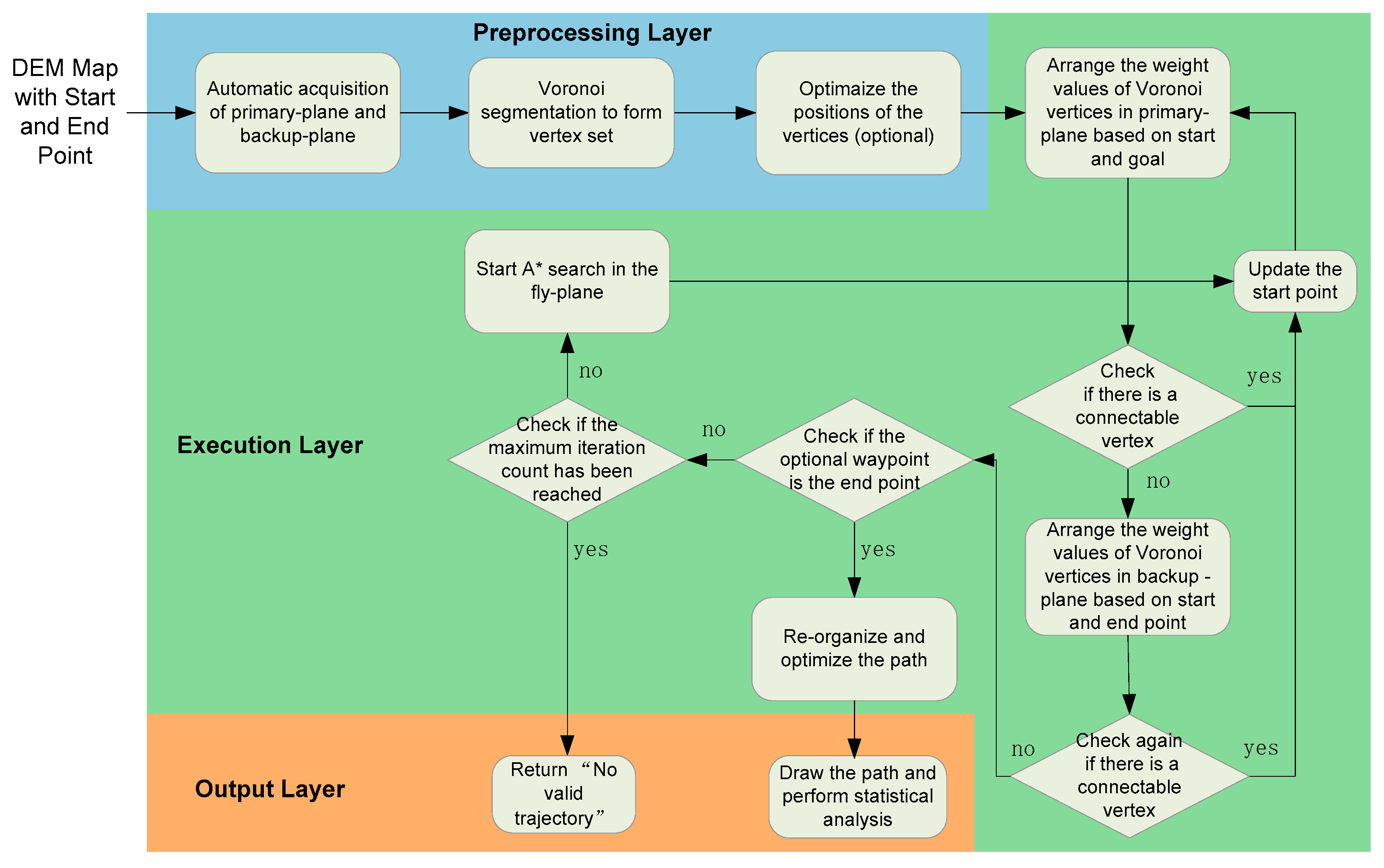
The remainder of this study is organized as follows: Section 2 reviews the foundational methodologies relevant to the proposed algorithm, encompassing DEM-based adaptive layering strategies, regional Voronoi vertex search diagrams, A* searches, and their hybrid integration for trajectory planning. Section 3 elaborates on the framework and operational workflow of the proposed algorithm, which enables rapid trajectory planning through a combination of multiple algorithms. Section 4 presents simulation experiments that validate the efficacy and computational efficiency of the fusion algorithm in mountainous terrain. The subsequent sections comparatively analyze algorithmic performance and explore potential research extensions. Finally, the conclusive findings are summarized.

2. Methodology

2.1. Adaptive DEM Flight Space Layering Model

DEM is a mathematical expression of the true three-dimensional shape of Earth’s surface. It is a type of physical ground model that represents ground elevation information through a set of ordered numerical arrays. In the field of UAV flight path planning, it serves as fundamental data. It can intuitively and realistically depict the geographical features of the UAV’s flight environment. The DEM represents terrain surface features through a discrete elevation data matrix, and its mathematical expression can be defined as follows:

$$DEM=\left\{Z_{i\mathrm{j}}\right\}i=\mathrm{1,2},\dots ,mj=\mathrm{1,2},\dots ,n$$

(1)

In this context, $Z_{i\mathrm{j}}$ represents the height value of the grid points i and j in the matrix, and $\mathrm{m} \mathrm{a}\mathrm{n}\mathrm{d} \mathrm{n}$ represent the spatial resolution of the regular grid. Compared to Digital Terrain Models (DTMs), DEMs specifically refer to elevation datasets without features, whereas DTMs also include derived terrain parameters, such as the slope and aspect. This distinction is particularly important in complex navigation, as pure elevation data are more conducive to geometric calculations for real-time path planning.

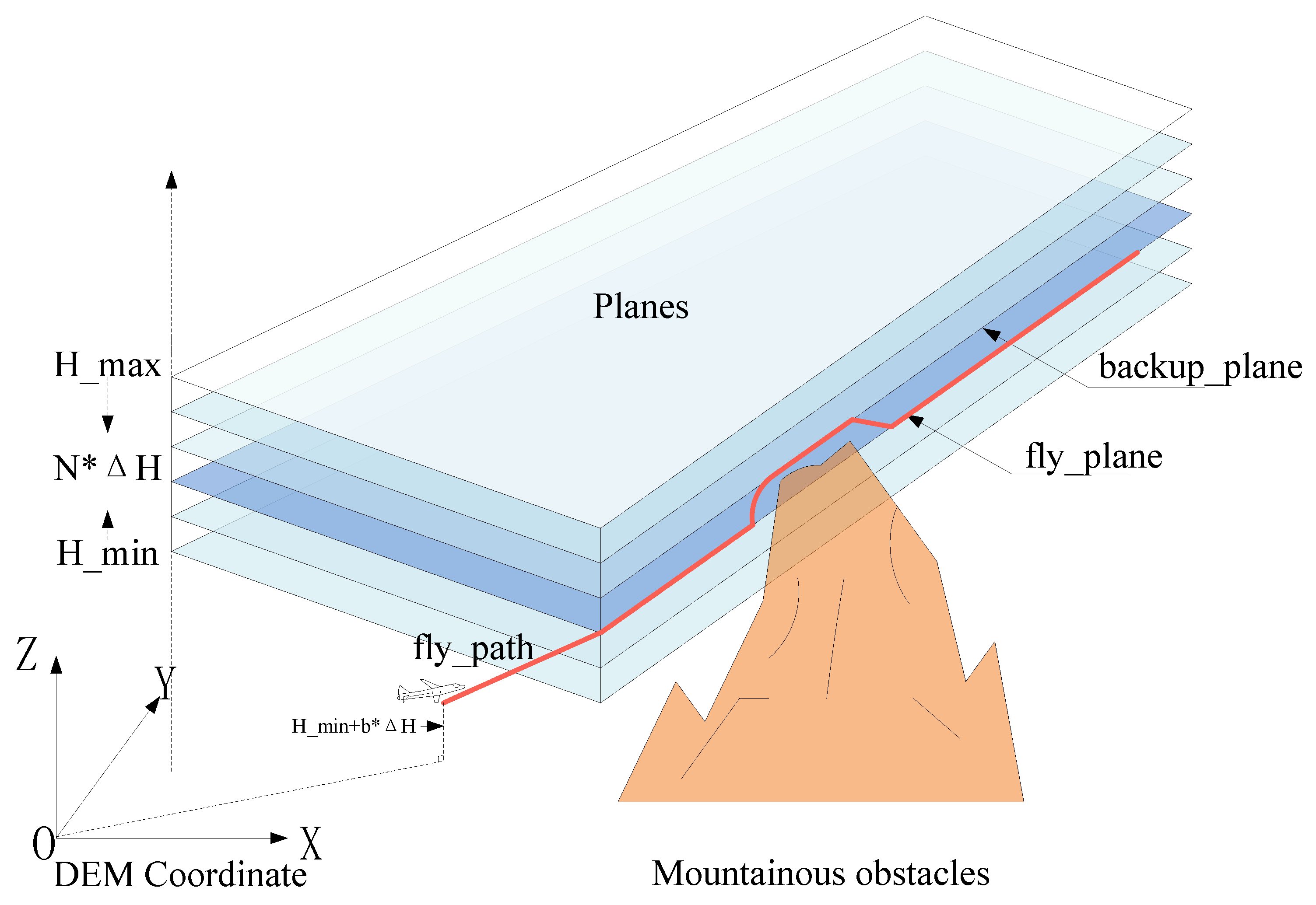
By incorporating DEM data, three-dimensional path planning can be achieved. However, due to the expansion of the search space dimensions, a significant increase in computational load occurs. In cases in which the scale of regional drones is controllable or the flying altitude is substantially higher than the obstacle requirements, DEM layering operations can transform the three-dimensional planning into two-dimensional planning, thereby simplifying the computational load. However, when drones fly through complex mountainous environments, this simplification results in increased path searching consumption due to insufficient two-dimensional information. Based on this, this study combines the flight performance of drones with an adaptive optimal flight level selection method, using adjacent higher layers as alternative obstacle avoidance layers to enable three-dimensional planning. This approach can minimize the computational load while retaining the advantages of three-dimensional paths.

For a given drone flight altitude range [$H_{min},H_{max}$] and the stratified altitude $∆\mathrm{H}$, a set of drone flight stratification thresholds is defined as follows:

$$H={\left\{H_p\right|H_p=H_{min}+p\times ∆H\}}_{p=0}^N$$

(2)

As indicated by the formula, the selection of $∆\mathrm{H}$ directly determines the number of vertical layers. This parameter should be maximized under the constraint that the aircraft’s inter-layer transition capability must be satisfied within a unit distance, thereby minimizing the computational and memory overhead caused by excessive layering, as shown in Figure 1.

Among them, N represents the number of layers, and its mathematical expression is shown as follows:

$$N=\mathrm{r}\mathrm{o}\mathrm{u}\mathrm{n}\mathrm{d}\left({\displaystyle \frac{{H_{max}-H}_{min}}{∆\mathrm{H}}}\right)$$

(3)

If the drone is flying at the k-th level, this means its flight altitude $D\left(i,j\right)$ lies between two adjacent height planes.

$$L_k=\left\{\left(i,j\right)|H_k\le D(i,j)<H_{k+1}\right\},k=\mathrm{1,2},\dots ,N-1$$

(4)

The mathematical expression for the set of terrain obstacles at flight level k is as follows:

$${Obs}_k=\left\{{\left(i,j\right)|Obs}_k\left(i,j\right)=\left\{\begin{array}{c}1,\\ 0,\end{array}\right.{\displaystyle \genfrac{}{}{0pt}{}{Z_{ij}\ge H_k}{Z_{ij}<H_k}}\right\},k=\mathrm{1,2},\dots ,N-1$$

(5)

There are two criteria for selecting the flight level: on the one hand, the flight level should be as low as possible to minimize energy consumption; on the other hand, obstacles should be avoided. However, these two points are contradictory in real-world scenarios. To solve this problem, this study proposes selecting the optimal drone cruising altitude based on the obstacle density value. The definition of obstacle density at a given altitude is as follows:

$${Dens}_k={\displaystyle \frac{{\sum }_{i=0}^m{\sum }_{j=0}^n{Obs}_k\left(i,j\right)}{m\times n}},k=\mathrm{1,2},\dots ,N-1$$

(6)

The physical meaning of the above equation refers to the percentage of the obstacle occupying the assigned cruising altitude.

The $Dens$ threshold parameter exhibits the following trade-offs:

A higher $Dens$ threshold prioritizes stealth by selecting flight planes closer to the terrain base, but this increases obstacle density and may render path planning infeasible.

A lower $Dens$ threshold improves path optimality by selecting higher-altitude flight planes (reducing obstacles) at the cost of increased detection risks.

By reasonably selecting the $Dens$ threshold, the corresponding optimal fly_plane $L_b$ can be obtained, with b representing the serial number of the best cruising level. The next higher level serves as the backup_plane used for obstacle avoidance when crossing mountainous terrain. To reduce the computational load, the layered obstacle density calculation begins at $H_{max}$ and approaches $H_{min}$ in increments of $∆\mathrm{H}$.

2.2. Voronoi Vertex-Based Search Model Based on Weight-Based Heuristic

A Voronoi diagram is used to divide space into several regions based on the principle of minimum distance. The core idea is that any point within a region should be closer to its corresponding generating object than to any other generating object [38]. In this design, obstacles within the flight layer selected through the adaptive DEM method are utilized as Voronoi objects for vertex generation. The Voronoi vertex generation algorithm proceeds through the following steps.

In the corresponding 2D terrain profile of the flight level, obstacles are classified according to their position $G=\{g_1,g_2,\dots ,g_n\}$, and Voronoi vertices are generated at loci equidistant to multiple obstacles, which are defined by the following.

For any pixel $\mathrm{p}$ in the image,

$$\mathrm{D}\mathrm{T}\left(\mathrm{p}\right)=\underset{q\in G}{\min }‖p-q‖$$

(7)

where $‖p-q‖$ is the Euclidean distance between $p$ and obstacle pixel $q$.

The vertex $v$ satisfies

$$\exists g_{\mathrm{i}},g_{\mathrm{j}}\subseteq G\left(i\ne j\right):\mathrm{D}\mathrm{T}\left(v,g_{\mathrm{i}}\right)=\mathrm{D}\mathrm{T}\left(v,g_{\mathrm{j}}\right) \wedge ‖\nabla DT\left(v\right)‖\approx 0$$

(8)

$v$ is equidistant to at least two obstacles and lies at the local maxima of DT.

$\nabla \mathrm{D}\mathrm{T}=({\displaystyle \frac{\partial DT}{\partial x}},{\displaystyle \frac{\partial DT}{\partial y}})$ is the gradient field at point $\left(x,\mathrm{y}\right)$.

Candidate vertices, $V_{candidate}$, are then identified, where the gradient magnitude approaches zero, shown as follows:

$$V_{candidate}=\left\{p\right|‖\nabla DT\left(p\right)‖<\epsilon \} (\epsilon \approx {10}^{-3})$$

(9)

Finally, vertices that only retain the local maxima in $\mathrm{D}\mathrm{T}$ are filtered as follows:

$$V_{final}=\{v\in V_{candidate}|DT\left(v\right)>DT\left(q\right),\forall \mathrm{q}\in N_8\left(\mathrm{v}\right)\}$$

(10)

where $N_8\left(v\right)$ denotes the 8-neighborhood value of $v$.

The proposed method’s advantage in trajectory planning is a result of its ability to generate a trajectory in a two-dimensional plane with distances equal to the obstacles, a feature that is particularly important in mountainous environments. Typically, there are valleys and plains between two mountain peaks, which means that the generated route points will have the maximum distance from the obstacles, thus avoiding collisions and ensuring higher safety in the generated flight path.

There are two key elements in the planar image processed using the Voronoi algorithm. One is the set of edges that divides the obstacles, and the other is the set of vertices where these edges intersect. In the field of route planning, the traditional approach is to generate trajectories along the Voronoi edges, followed by turn optimization. This method often results in longer and less-direct routes. We construct a new discrete search space based on the vertices of the Voronoi diagram formed at the flight altitude, assigning weights to all points within this search space and then performing a ranked search. The discrete search space $\mathrm{V}\mathrm{e}\mathrm{c}$ is defined as follows:

$$\mathrm{V}\mathrm{e}\mathrm{c}=\{\mathrm{s}\mathrm{t}\mathrm{a}\mathrm{r}\mathrm{t},v_1,v_2,\dots v_p,\mathrm{e}\mathrm{n}\mathrm{d}\}$$

(11)

Among them, $\mathrm{s}\mathrm{t}\mathrm{a}\mathrm{r}\mathrm{t}$ represents the starting point of the flight plan, $\mathrm{e}\mathrm{n}\mathrm{d}$ represents the ending point of the flight plan, and $p$ refers to the number of vertices in the set after Voronoi processing.

Based on the current step’s starting and ending point information, the heuristic weight values for all vertices, $v_{\mathrm{p}}$, are calculated. Then, all feature points that have no obstacles along the line connecting them to the current starting point are filtered out, and they are subsequently sorted according to their weights. The feature point with the highest weight is selected, and it is connected to the starting point, rendering this vertex the new starting point for the next iteration.

The heuristic weight value $h_{\mathrm{p}}$ of each Voronoi vertex $v_{\mathrm{p}}$ in the computational graph is calculated, and verification is carried out to ensure that there is no obstruction in the line connecting the vertices and the current planning starting point. The weight formula is defined as follows:

$${h_{\mathrm{p}}=w}_1\times {\displaystyle \frac{{ds}_p}{\mathrm{d}\mathrm{m}\mathrm{a}\mathrm{x}}}+w_2\times \mathrm{e}\mathrm{x}\mathrm{p}\left(-1\times \left({\displaystyle \frac{{\mathrm{d}\mathrm{g}}_p}{\mathrm{d}\mathrm{m}\mathrm{a}\mathrm{x}}}\right)\right)+w_3\times \mathrm{e}\mathrm{x}\mathrm{p}\left(-1\times \left({\displaystyle \frac{{\mathrm{t}\mathrm{h}\mathrm{e}\mathrm{t}\mathrm{a}}_p}{\mathrm{p}\mathrm{i}}}\right)\right)+w_4\times {\displaystyle \frac{{{\mathrm{h}}_{\mathrm{v}\mathrm{e}\mathrm{c}}}_p}{H_{max}}}$$

(12)

If there is any obstruction, then $h_{\mathrm{p}}=0$.

Among them, ${ds}_p$ represents the distance from the current vertex to the planned starting point, $\mathrm{d}\mathrm{m}\mathrm{a}\mathrm{x}$ represents the distance between the start and end points, ${\mathrm{d}\mathrm{g}}_p$ represents the distance from the vertex to the end point, and ${\mathrm{t}\mathrm{h}\mathrm{e}\mathrm{t}\mathrm{a}}_p$ represents the angle between the vector from the current vertex to the starting point and the vector from the current vertex to the ending point. pi is a constant, ${\mathrm{h}\_\mathrm{v}\mathrm{e}\mathrm{c}}_p$ represents the height from the vertex to the ground, and $H_{max}$ represents the maximum flying height of the drone.

The weighting parameters are defined as follows:

$w_1$: Path proximity-to-origin weight.

Increasing this value prioritizes waypoints closer to the starting point, preventing premature deviations from the initial heading.

$w_2$: Path proximity-to-goal attenuation weight.

Higher values emphasize feature points near the destination, accelerating the terminal approach.

$w_3$: Path directional consistency weight.

Enhanced weighting selects waypoints that maintain heading alignments, reducing course oscillations.

$w_4$: Flight altitude safety margin weight.

Increased weighting favors waypoints with greater vertical clearance from terrain/obstacles.

The sum of the four weights is designed to equal 1. In this algorithm, $w_1$ is 0.1, $w_2$ is 0.3, $w_3$ is 0.5, and $w_4$ is 0.1.

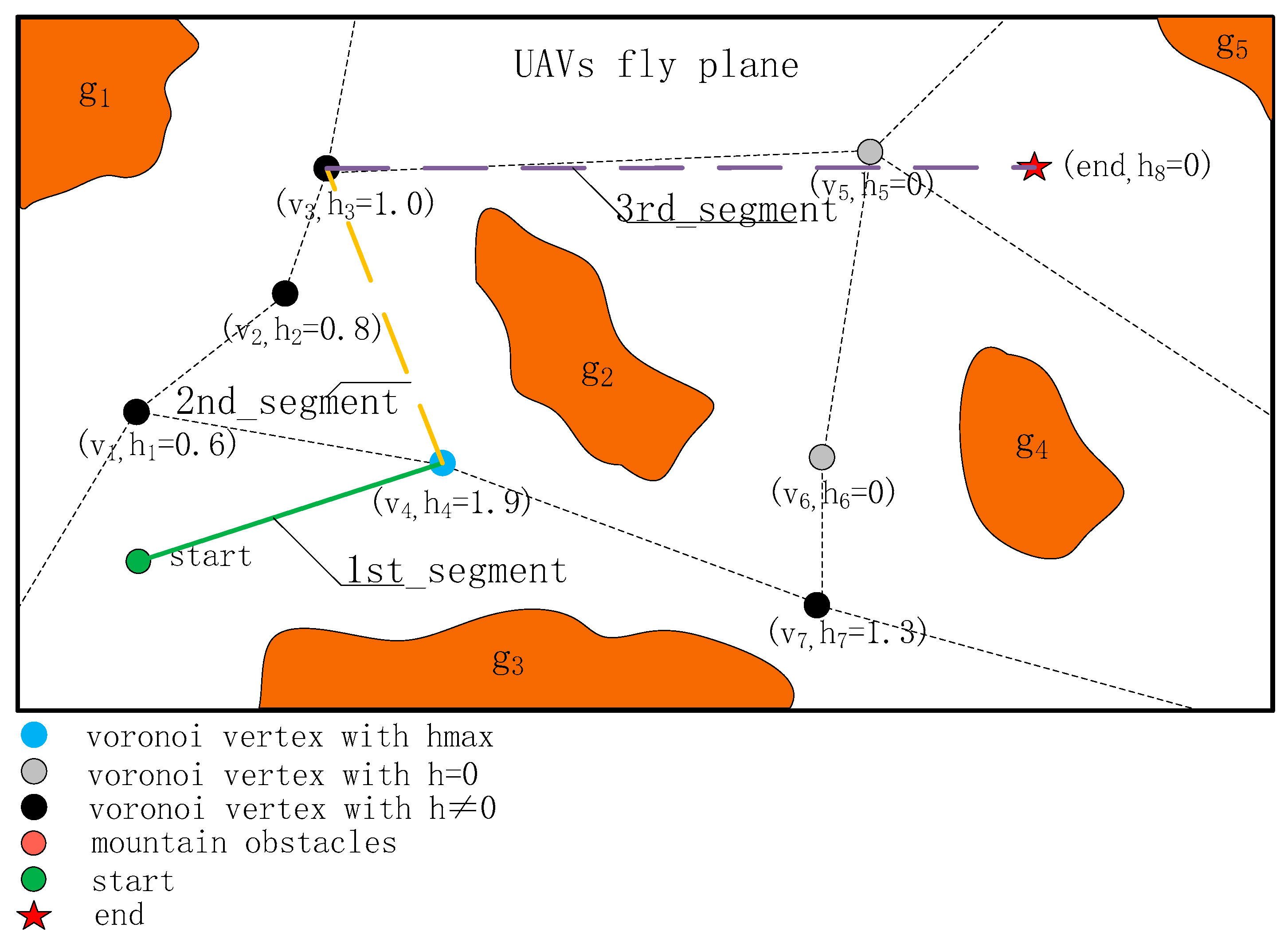
The Voronoi vertex $h_{\mathrm{m}\mathrm{a}\mathrm{x}}$ corresponding to the largest value in the sequence is selected, and $h_{\mathrm{p}}$ is the next waypoint connected to the current starting point. The Euclidean distance between this vertex and the planned endpoint is recorded as $D=|v_{\mathrm{m}\mathrm{a}\mathrm{x}}-end|$. Then, this vertex is updated as the new search starting point, the original starting point is removed from the search space, the weights are recalculated, and the vertex with the decreased $D \mathrm{v}\mathrm{a}\mathrm{l}\mathrm{u}\mathrm{e}$ is selected; this process is then repeated until the planned endpoint is found.

The schematic of the rapid path search method using Voronoi vertices is shown in Figure 2. By iteratively selecting ${start,v}_4{,v}_3,\mathrm{a}\mathrm{n}\mathrm{d} end$ as waypoints, a quick generation of the UAV’s trajectory within the flight plane is achieved.

2.3. A* Algorithm for Route Segment Connection

By utilizing Voronoi-vertex-based search models, drones can already plan feasible flight routes in certain scenarios. For instance, in Figure 3, a flyable path can be determined using only three line segments. However, as the complexity of obstacles increases, situations where it is impossible to quickly generate paths using existing vertices may arise. In such cases, all Voronoi vertices within the known search space have a weight value of 0, or the distance values, $D$, no longer decrease. Typically, at this point, the starting point has advanced closer to the planned endpoint from its initial position, necessitating an extension of the trajectory to obtain new connectable Voronoi vertices and thereby transforming the problem into a local trajectory search method.

The A* algorithm is a classic heuristic search algorithm. The heuristic function is calculated based on the minimum objective function value from the starting point to the current node combined with the estimated function value from the current node to the target point [39]. The entire trajectory search relies on this heuristic function. In a two-dimensional plane, the search space of the A* algorithm typically consists of the 8 pixels surrounding the current point. For each pixel in the search space, the cost is computed, and the node with the lowest cost is selected and added to the path as the new starting point. The cost function for node M in the search space is defined as follows:

$$f\left(M\right)=g\left(M\right)+h\left(M\right)$$

(13)

where, $g\left(M\right)$ represents the heuristic factor, indicating the true cost from the initial node to the current node M, and $h\left(M\right)$ represents the minimum cost estimate from the current node M to the target node. The search principle is to prioritize expanding nodes with lower $f\left(M\right)$ values, which guarantees finding the optimal path. Generally, the A* algorithm demonstrates superior pathfinding performance and high robustness. However, in global route planning, due to the increase in search area, obtaining an optimal path requires a long convergence time and substantial memory space. However, by introducing a quick search strategy based on Voronoi vertices, the search and computation time can be significantly reduced. At this point, the A* algorithm serves as a localized searching algorithm for existing segments. As the search principle of the A* algorithm is well-established, this study does not elaborate on this topic further. We only provide an example of the initiation timing of the A* algorithm as a connection algorithm for route segments.

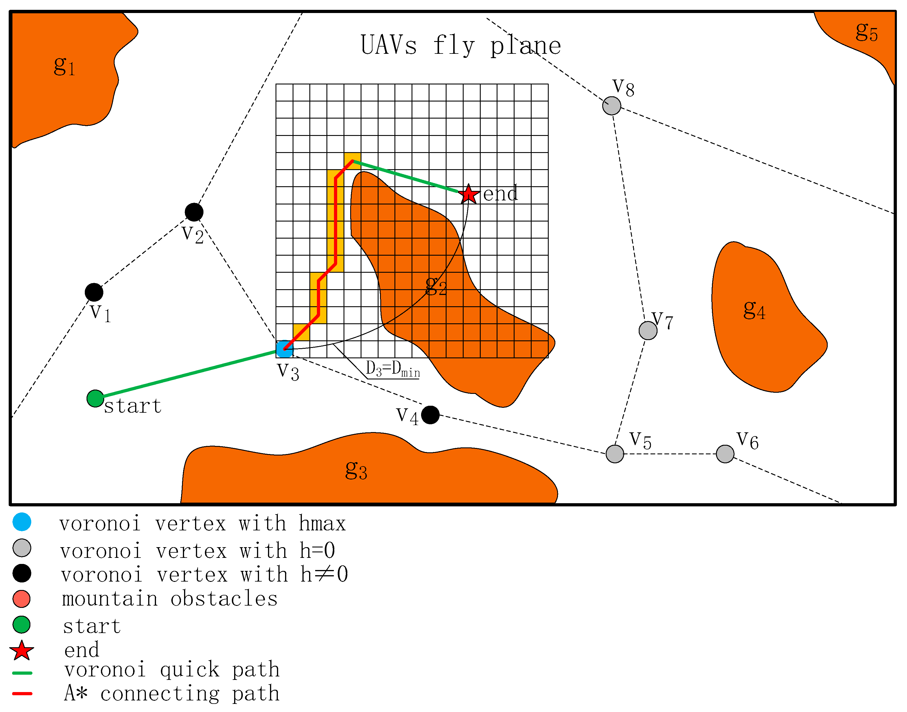
The connection of flight route segments using the A* algorithm is shown in Figure 4. After the UAV reaches the point $v_3$ by rapidly searching the path through the Voronoi vertices, with point $v_3$ as the new starting point, the only directly connectable Voronoi vertices are $v_1{, v}_2{, \mathrm{a}\mathrm{n}\mathrm{d} v}_4$. By comparing the distance to the endpoint vector, point $v_3$ is already the nearest connectable Voronoi vertex to the end point. At this point, the A* search mechanism is introduced, and the local path toward the endpoint is generated as a connection path, continuing until a new starting point appears in the A* path, where a new quick connection path can be generated in the search space.

2.4. Optimization of Flight Path

The standard process for general UAV flight path planning typically consists of the following three steps: (1) modeling the flight environment space, (2) connecting the starting point and endpoint using a routing algorithm to form an initial flight path, and (3) further optimizing the initial flight path [40].

• Interpolation Optimization of Flight Path

The fast search based on Voronoi vertices is a sparse search process with the advantage of high search speeds; this is highly practical when the UAV has sufficient endurance. However, the disadvantage is that it cannot compare with heuristic algorithms in generating flight paths with optimization goals. However, the waypoints based on the fast search model still have significant optimization potential.

The flight path generated after the search is as follows:

$$P={\bigcup }_{i=1}^n\overline{P_{i-1}{P}_i}$$

(14)

where $\overline{{\mathrm{P}}_{\mathrm{i}-1}{\mathrm{P}}_{\mathrm{i}}}$ is the line segment connecting the points ${\mathrm{P}}_{\mathrm{i}-1}$ and ${\mathrm{P}}_{\mathrm{i}}$.

Fixed-distance interpolation is performed on this segment to generate a new set of interpolation points, as follows:

$$Q_i=\left\{q_{i,k}=P_{i-1}+k·\delta ·u_i\right|k=\mathrm{0,1},\dots \dots m_i\}$$

(15)

where $u_i={\displaystyle \frac{P_i-P_{i-1}}{‖P_i-P_{i-1}‖}}$ represents the direction of the unit vector, and $m_i=⌊{\displaystyle \frac{‖P_i-P_{i-1}‖}{\delta }}⌋$ represents the number of points after the interpolation of the line segment.

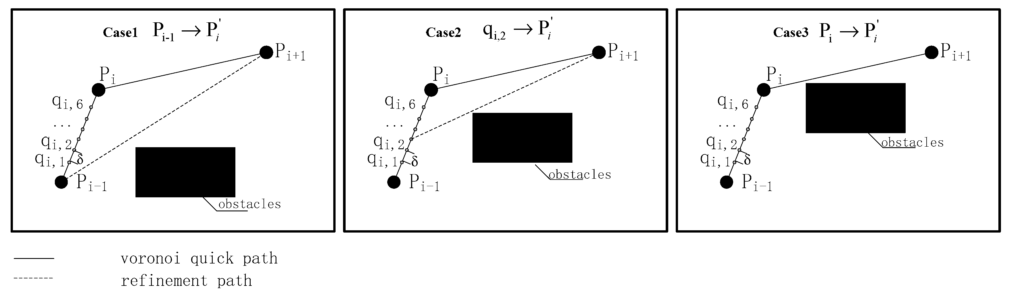
The sequence of the flight path segment $Q_i$ is followed to detect the point $q_{i,k}$ in the area. If there is no collision in $\overline{q_{i,k}{P}_{i+1}}$, then point $q_{i,k}$ is added to list $P^{\prime }$. If no $q_{i,k}$ values meet the conditions, then $P_i$ is retained and added to the $P^{\prime }$ list.

The value of ${P^{\prime }}_i$ is updated to $P_i$, and interpolation searches are continually performed on $\overline{P_i{P}_{i+1}}$ until the endpoint $P_n$ is added to $P^{\prime }$.

Compared to the initial flight path, this optimization method allows for the reconstruction of the path, ensuring that the new trajectory connects both the starting and ending points, with each segment of the sub-path avoiding obstacles; moreover, the total path is as short as possible, as illustrated in Figure 5.

2.

Optimization of the Position of Voronoi Vertices

In theory, the vertices obtained after Voronoi division are the farthest from obstacles in the horizontal space, providing a higher safety margin. However, this approach does not take into account the altitude relative to the ground when UAVs fly in complex mountainous environments. Height measurements can be carried out at the vertices and their neighbors using planar detection, and the point with the largest height margin can be selected as the optimized point for use.

The vertex optimization method involves generating a candidate set $P_{ij}$ for each initial vertex $P_i\in Vec$ by performing a plane rasterization process.

$$P_{ij}=\left\{P_{ij}\right| j\in \left[1,N\right],N={round(\left(R÷L\right)}^2\left)\right\}$$

(16)

Here, $R$ represents the neighborhood search radius, $L$ represents the elevation data scale, and $N$ represents the number of search points.

The safety margin for elevation is calculated at each point in the search area as follows:

$$∆h_{ij}=\mathrm{h}-h_{ij}$$

(17)

where $h_{ij}$ is the height value corresponding to the point in the DEM, while $\mathrm{h}$ denotes the height of the current flight plane.

The principle of safety margin maximization is adopted as follows:

$${\mathrm{P}}_i^{\prime }=\max \left(∆h_{ij}\right),\forall j\in \left\{j\right|∆h_{ij}>0\}$$

(18)

The optimized vertices are then updated to the new Voronoi vertex set. By establishing the vertex optimization mechanism, the altitude margin for drone flights is significantly improved, making the flight path more reliable. However, the optimization process is computationally intensive and dependent on the search design, introducing additional computational loads. In time-sensitive planning scenarios, this optimization option can be disabled.

2.5. Complexity Analysis

According to the algorithm’s design, the proposed method primarily consists of the following key components: Voronoi vertex acquisition, heuristic-based vertex selection, A* connection, and interpolation-based path optimization. The theoretical computational complexity analysis of these components is as follows.

The computational complexity of Voronoi vertex acquisition is $\mathrm{O}(\left(\mathrm{M}\times \mathrm{N}\right)·\mathrm{l}\mathrm{o}\mathrm{g}(\mathrm{M}\times \mathrm{N}\left)\right)$, where $\mathrm{M}$ and $\mathrm{N}$ denote the width and height of the flight plane map, respectively, corresponding to a space complexity of $\mathrm{O}(\mathrm{M}\times \mathrm{N})$.

Assuming that the number of vertices in the Voronoi diagram on the map is $\mathrm{Q}$, the heuristic-based vertex selection method exhibits a computational complexity of $\mathrm{O}(\mathrm{Q}·\mathrm{l}\mathrm{o}\mathrm{g}\left(\mathrm{Q}\right))$ and a space complexity of $\mathrm{O}\left(\mathrm{Q}\right)$.

The A* connection algorithm exhibits a computational and space complexity of $\mathrm{O}(\mathrm{b}^\mathrm{d})$, where $\mathrm{b}$ denotes the branching factor (number of expanded nodes per level) and $\mathrm{d}$ represents the depth of the optimal path segment. The proposed Voronoi–A* framework strategically applies A* only to short path segments, where the limited depth $\mathrm{d}$ guarantees low computational complexity.

The interpolation-based path optimization has a computational complexity of $\mathrm{O}\left(\mathrm{P}\right)$ and a space complexity of $\mathrm{O}\left(\mathrm{P}\right)$, where $\mathrm{P}$ denotes the number of interpolation points along the path.

The algorithm demonstrates well-bounded computational and space complexity. The Voronoi vertex acquisition stage dominates the overall cost with a time complexity of $\mathrm{O}(\left(\mathrm{M}\times \mathrm{N}\right)·\mathrm{l}\mathrm{o}\mathrm{g}(\mathrm{M}\times \mathrm{N}\left)\right)$ and a space complexity of $\mathrm{O}(\mathrm{M}\times \mathrm{N})$. Subsequent heuristic-based vertex selection operates at $\mathrm{O}(\mathrm{Q}·\mathrm{l}\mathrm{o}\mathrm{g}\left(\mathrm{Q}\right))$ time complexity and $\mathrm{O}\left(\mathrm{Q}\right)$ space complexity, while localized A* connections maintain manageable $\mathrm{O}(\mathrm{b}^\mathrm{d})$ complexity through constrained path segments. The final path optimization only requires linear $\mathrm{O}\left(\mathrm{P}\right)$ time/space complexity. This phased complexity design ensures efficient scalability, while initial map processing requires more computation, with subsequent steps slowly increasing in computational demands, maintaining high efficiency even when handling large-scale problems.

3. Algorithm Design: Hybrid Voronoi–A* Framework and Pseudocode

After the above research, a combined Voronoi–A* algorithm is designed to meet the route planning needs of drones in complex mountainous environments. The main steps of the proposed algorithm are as follows: (1) By utilizing the obstacle density information from the DEM layer, the drone’s primary flight level and a higher backup obstacle avoidance layer are adaptively selected, producing a three-dimensional trajectory. (2) The Voronoi method is applied to process the flight level, and the Voronoi vertex set of that level is obtained, serving as a point set for fast path search space. (3) Based on weight designs, the weight of each Voronoi vertex is calculated, and after sorting, the highest-weighted point is added to the path. (4) If no additional Voronoi vertex can be connected at the current flight level, then the algorithm attempts to switch to a higher level to query Voronoi vertices, continuing the fast connection. If it fails, then A* is activated at the flight level to expand the route. Then, steps (3) and (4) are repeated until the destination is added to the route points. (5) To address redundant sparse path points and excessive turning angles, interpolation and optimization are performed on the route. (6) The optimized route is then output as the primary flight route for drones in mountainous terrain. Due to the use of a combined layered obstacle avoidance and A* expansion strategy, this path can quickly generate flyable routes while avoiding obstacles in complex mountainous environments, and the algorithm exhibits a high degree of safety and robustness. The pseudocode and flowchart for the hybrid Voronoi–A* algorithm are presented in Algorithm 1 and Figure 6, respectively.

Algorithm 1 Voronoi and A* hybrid algorithm pseudocode

Three-Dimensional UAV Path Planning via Hybrid Voronoi and A* Approach

Input: $\mathrm{DEM}\mathrm{Z}\in {\mathrm{R}}^{\mathrm{H}\times \mathrm{W}}$$, \mathrm{Start} \mathrm{point} {\mathrm{p}}_{\mathrm{s}}=({\mathrm{x}}_{\mathrm{s}},{\mathrm{y}}_{\mathrm{s}})$$\mathrm{Goal} \mathrm{point} {\mathrm{p}}_{\mathrm{g}}=({\mathrm{x}}_{\mathrm{g}},{\mathrm{y}}_{\mathrm{g}})$ $\mathrm{Parameters}: \mathrm{Obstacle} \mathrm{dense} \mathrm{threshold} \mathrm{\beta }=0.25$$, \mathrm{Scale} \mathrm{factor} \mathrm{\alpha }=0.2$, $\mathrm{DEM} \mathrm{Layer} \mathrm{Number} \mathrm{L}=20$$, \mathrm{Safe} \mathrm{Window} \mathrm{Size} \mathrm{w}=0.25$, $\mathrm{Max} \mathrm{iteration} \mathrm{number} \mathrm{I}\mathrm{t}\mathrm{e}\mathrm{r}\_\mathrm{m}\mathrm{a}\mathrm{x}=20$ Output: $\mathrm{Optimized} \mathrm{path} \mathrm{P}=\{{\mathrm{p}}_{\mathrm{s}},{\mathrm{p}}_1,{\mathrm{p}}_2\dots {,{\mathrm{p}}_{\mathrm{n}},\mathrm{p}}_{\mathrm{g}}\}$

1: Preprocessing 2: $\mathrm{Z}\leftarrow \mathrm{r}\mathrm{e}\mathrm{s}\mathrm{i}\mathrm{z}\mathrm{e}\left(\mathrm{Z},\mathrm{\alpha }\right):\mathrm{S}\mathrm{c}\mathrm{a}\mathrm{l}\mathrm{e} \mathrm{m}\mathrm{a}\mathrm{p}$ 3: ${\mathrm{Z}}_{\mathrm{m}\mathrm{a}\mathrm{x}}\leftarrow \max \left(\mathrm{Z}\right),{\mathrm{Z}}_{\mathrm{m}\mathrm{i}\mathrm{n}}\leftarrow \min \left(\mathrm{Z}\right)$ 4: $∆\mathrm{H}\leftarrow ({\mathrm{Z}}_{\mathrm{m}\mathrm{a}\mathrm{x}}-{\mathrm{Z}}_{\mathrm{m}\mathrm{i}\mathrm{n}})/\mathrm{L}$ 5: $\mathrm{f}\mathrm{o}\mathrm{r}\mathrm{k}=1\mathrm{t}\mathrm{o} \mathrm{L}\mathrm{d}\mathrm{o}$ 6: ${\mathrm{O}\mathrm{b}\mathrm{s}}_{\mathrm{k}}\leftarrow \left\{\left(\mathrm{i},\mathrm{j}\right)∣\mathrm{Z}\left(\mathrm{i},\mathrm{j}\right)\ge {\mathrm{Z}}_{\min }+\left(\mathrm{k}-1\right)∆\mathrm{H}\right\}:\mathrm{O}\mathrm{b}\mathrm{s}\mathrm{t}\mathrm{a}\mathrm{c}\mathrm{l}\mathrm{e} \mathrm{s}\mathrm{e}\mathrm{t}$ 7: $\mathrm{i}\mathrm{f} {\mathrm{O}\mathrm{b}\mathrm{s}}_{\mathrm{k}}/\left(\mathrm{H}\mathrm{W}\right)<\beta then$ 8: ${\mathrm{h}}_{\mathrm{f}\mathrm{l}\mathrm{y}}\leftarrow {\mathrm{Z}}_{\mathrm{m}\mathrm{i}\mathrm{n}}+\left(\mathrm{k}-1\right)∆\mathrm{H}\hspace{1em}:\mathrm{S}\mathrm{e}\mathrm{l}\mathrm{e}\mathrm{c}\mathrm{t} \mathrm{p}\mathrm{r}\mathrm{i}\mathrm{m}\mathrm{a}\mathrm{r}\mathrm{y} \mathrm{f}\mathrm{l}\mathrm{i}\mathrm{g}\mathrm{h}\mathrm{t} \mathrm{h}\mathrm{e}\mathrm{i}\mathrm{g}\mathrm{h}\mathrm{t}$ 9: ${\mathrm{h}}_{\mathrm{b}\mathrm{a}\mathrm{k}}\leftarrow {\mathrm{Z}}_{\mathrm{m}\mathrm{i}\mathrm{n}}+\left(\mathrm{k}\right)∆\mathrm{H}:\mathrm{S}\mathrm{e}\mathrm{l}\mathrm{e}\mathrm{c}\mathrm{t} \mathrm{b}\mathrm{a}\mathrm{c}\mathrm{k}\mathrm{u}\mathrm{p} \mathrm{f}\mathrm{l}\mathrm{i}\mathrm{g}\mathrm{h}\mathrm{t} \mathrm{h}\mathrm{e}\mathrm{i}\mathrm{g}\mathrm{h}\mathrm{t}$ 10: break 11: Voronoi Vertex Extraction 12: $\mathrm{V}\leftarrow \mathrm{V}\mathrm{o}\mathrm{r}\mathrm{o}\mathrm{n}\mathrm{o}\mathrm{i}\left({\mathrm{O}\mathrm{b}\mathrm{s}}_{\mathrm{k}}\right) :\mathrm{G}\mathrm{e}\mathrm{n}\mathrm{e}\mathrm{r}\mathrm{a}\mathrm{t}\mathrm{e} \mathrm{V}\mathrm{o}\mathrm{r}\mathrm{o}\mathrm{n}\mathrm{o}\mathrm{i} \mathrm{d}\mathrm{i}\mathrm{a}\mathrm{g}\mathrm{r}\mathrm{a}\mathrm{m}$ 13: $\mathrm{V}\mathrm{e}\mathrm{x}\leftarrow \{{\mathrm{p}}_{\mathrm{s}},{\mathrm{p}}_{\mathrm{g}}\}:\mathrm{I}\mathrm{n}\mathrm{i}\mathrm{t}\mathrm{i}\mathrm{a}\mathrm{l}\mathrm{i}\mathrm{z}\mathrm{e} \mathrm{w}\mathrm{i}\mathrm{t}\mathrm{h} \mathrm{s}\mathrm{t}\mathrm{a}\mathrm{r}\mathrm{t}/\mathrm{g}\mathrm{o}\mathrm{a}\mathrm{l}$ 14: $\mathrm{f}\mathrm{o}\mathrm{r} \mathrm{e}\mathrm{a}\mathrm{c}\mathrm{h} \mathrm{v}\mathrm{e}\mathrm{r}\mathrm{t}\mathrm{e}\mathrm{x} {\mathrm{v}}_{\mathrm{i}}\in \mathrm{V} \mathrm{d}\mathrm{o}$ 15: $\mathrm{i}\mathrm{f}{\mathrm{v}}_{\mathrm{i}}\mathrm{i}\mathrm{s} \mathrm{i}\mathrm{n}\mathrm{s}\mathrm{i}\mathrm{d}\mathrm{e} \mathrm{m}\mathrm{a}\mathrm{p} \mathrm{a}\mathrm{n}\mathrm{d}\mathrm{c}\mathrm{l}\mathrm{e}\mathrm{a}\mathrm{r}\mathrm{a}\mathrm{n}\mathrm{c}\mathrm{e}\left({\mathrm{v}}_{\mathrm{i}},\mathrm{w}\right)\mathrm{t}\mathrm{h}\mathrm{e}\mathrm{n} \mathrm{d}\mathrm{o}$ 16: $\mathrm{V}\mathrm{e}\mathrm{x}\leftarrow \mathrm{V}\mathrm{e}\mathrm{x}\cup {\mathrm{v}}_{\mathrm{i}}$ 17: Hybrid Path Search 18: $\mathrm{f}\mathrm{o}\mathrm{r}\mathrm{i}=1\mathrm{t}\mathrm{o} \mathrm{I}\mathrm{t}\mathrm{e}\mathrm{r}\_\mathrm{m}\mathrm{a}\mathrm{x}\mathrm{d}\mathrm{o}$ 19: ${\mathrm{P}}_{\mathrm{q}\mathrm{u}\mathrm{i}\mathrm{c}\mathrm{k}}\leftarrow \mathrm{G}\mathrm{r}\mathrm{e}\mathrm{e}\mathrm{d}\mathrm{y}\mathrm{C}\mathrm{o}\mathrm{n}\mathrm{n}\mathrm{e}\mathrm{c}\mathrm{t}\left(\mathrm{V}\mathrm{e}\mathrm{x},{\mathrm{O}\mathrm{b}\mathrm{s}}_{\mathrm{k}}\right):\mathrm{V}\mathrm{o}\mathrm{r}\mathrm{o}\mathrm{n}\mathrm{o}\mathrm{i}-\mathrm{v}\mathrm{e}\mathrm{r}\mathrm{t}\mathrm{e}\mathrm{x} \mathrm{p}\mathrm{r}\mathrm{i}\mathrm{m}\mathrm{a}\mathrm{r}\mathrm{y} \mathrm{f}\mathrm{a}\mathrm{s}\mathrm{t} \mathrm{p}\mathrm{a}\mathrm{t}\mathrm{h}$ 20:${\mathrm{P}}_{\mathrm{q}\mathrm{u}\mathrm{i}\mathrm{c}\mathrm{k}}\leftarrow \mathrm{G}\mathrm{r}\mathrm{e}\mathrm{e}\mathrm{d}\mathrm{y}\mathrm{C}\mathrm{o}\mathrm{n}\mathrm{n}\mathrm{e}\mathrm{c}\mathrm{t}\left(\mathrm{V}\mathrm{e}\mathrm{x},{\mathrm{O}\mathrm{b}\mathrm{s}}_{\mathrm{k}+1}\right):\mathrm{V}\mathrm{o}\mathrm{r}\mathrm{o}\mathrm{n}\mathrm{o}\mathrm{i}-\mathrm{v}\mathrm{e}\mathrm{r}\mathrm{t}\mathrm{e}\mathrm{x} \mathrm{b}\mathrm{a}\mathrm{c}\mathrm{k}\mathrm{u}\mathrm{p} \mathrm{f}\mathrm{a}\mathrm{s}\mathrm{t} \mathrm{p}\mathrm{a}\mathrm{t}\mathrm{h}$ 21:$\mathrm{i}\mathrm{f}{\mathrm{P}}_{\mathrm{q}\mathrm{u}\mathrm{i}\mathrm{c}\mathrm{k}}\mathrm{d}\mathrm{o}\mathrm{e}\mathrm{s} \mathrm{n}\mathrm{o}\mathrm{t} \mathrm{r}\mathrm{e}\mathrm{a}\mathrm{c}\mathrm{h}{\mathrm{p}}_{\mathrm{g}}\mathrm{t}\mathrm{h}\mathrm{e}\mathrm{n}$ 22:${\mathrm{P}}_{\mathrm{A}\mathrm{s}\mathrm{t}\mathrm{a}\mathrm{r}}\leftarrow \mathrm{A}\ast \left(\mathrm{l}\mathrm{a}\mathrm{s}\mathrm{t}\left({\mathrm{P}}_{\mathrm{q}\mathrm{u}\mathrm{i}\mathrm{c}\mathrm{k}}\right),{\mathrm{p}}_{\mathrm{g}},{\mathrm{O}\mathrm{b}\mathrm{s}}_{\mathrm{k}}\right):\mathrm{A}\mathrm{s}\mathrm{t}\mathrm{a}\mathrm{r} \mathrm{s}\mathrm{e}\mathrm{a}\mathrm{r}\mathrm{c}\mathrm{h} \mathrm{i}\mathrm{n} 2\mathrm{D} \mathrm{p}\mathrm{r}\mathrm{i}\mathrm{m}\mathrm{a}\mathrm{r}\mathrm{y} \mathrm{p}\mathrm{l}\mathrm{a}\mathrm{n}\mathrm{e}$ 23:$\mathrm{i}\mathrm{f}\mathrm{l}\mathrm{a}\mathrm{s}\mathrm{t}\left({\mathrm{P}}_{\mathrm{A}\mathrm{s}\mathrm{t}\mathrm{a}\mathrm{r}}\right)\mathrm{d}\mathrm{o}\mathrm{e}\mathrm{s} \mathrm{n}\mathrm{o}\mathrm{t} \mathrm{r}\mathrm{e}\mathrm{a}\mathrm{c}\mathrm{h}{\mathrm{p}}_{\mathrm{g}} \mathrm{a}\mathrm{n}\mathrm{d}$ 24:$\mathrm{G}\mathrm{r}\mathrm{e}\mathrm{e}\mathrm{d}\mathrm{y}\mathrm{C}\mathrm{o}\mathrm{n}\mathrm{n}\mathrm{e}\mathrm{c}\mathrm{t}\mathrm{J}\mathrm{u}\mathrm{d}\mathrm{g}\mathrm{e}\left(\mathrm{l}\mathrm{a}\mathrm{s}\mathrm{t}\left({\mathrm{P}}_{\mathrm{A}\mathrm{s}\mathrm{t}\mathrm{a}\mathrm{r}}\right),{\mathrm{V}\mathrm{e}\mathrm{x},\mathrm{O}\mathrm{b}\mathrm{s}}_{\mathrm{k}}\right)==\mathrm{t}\mathrm{r}\mathrm{u}\mathrm{e} \mathrm{t}\mathrm{h}\mathrm{e}\mathrm{n}$ 25:$\mathrm{P}\leftarrow {\mathrm{P}}_{\mathrm{q}\mathrm{u}\mathrm{i}\mathrm{c}\mathrm{k}}\oplus {\mathrm{P}}_{\mathrm{A}\mathrm{s}\mathrm{t}\mathrm{a}\mathrm{r}}:\mathrm{P}\mathrm{a}\mathrm{t}\mathrm{h} \mathrm{c}\mathrm{o}\mathrm{n}\mathrm{c}\mathrm{a}\mathrm{t}\mathrm{e}\mathrm{n}\mathrm{a}\mathrm{t}\mathrm{i}\mathrm{o}\mathrm{n}$ 26:$\mathrm{e}\mathrm{l}\mathrm{s}\mathrm{e} \mathrm{P}\leftarrow {\mathrm{P}}_{\mathrm{q}\mathrm{u}\mathrm{i}\mathrm{c}\mathrm{k}}\oplus {\mathrm{P}}_{\mathrm{A}\mathrm{s}\mathrm{t}\mathrm{a}\mathrm{r}}; \mathrm{b}\mathrm{r}\mathrm{e}\mathrm{a}\mathrm{k}$ 27:$\mathrm{e}\mathrm{l}\mathrm{s}\mathrm{e} \mathrm{P}\leftarrow {\mathrm{P}}_{\mathrm{q}\mathrm{u}\mathrm{i}\mathrm{c}\mathrm{k}}; \mathrm{b}\mathrm{r}\mathrm{e}\mathrm{a}\mathrm{k}$ 28: Path Optimization 29: $\mathrm{P}\leftarrow \mathrm{R}\mathrm{e}\mathrm{m}\mathrm{o}\mathrm{v}\mathrm{e}\mathrm{D}\mathrm{u}\mathrm{p}\mathrm{l}\mathrm{i}\mathrm{c}\mathrm{a}\mathrm{t}\mathrm{e}\mathrm{s}\left(\mathrm{P}\right)$ 30: $\mathrm{f}\mathrm{o}\mathrm{r}\mathrm{j}=1\mathrm{t}\mathrm{o}\mid \mathrm{P}\mid -1\mathrm{d}\mathrm{o}$ 31: $\mathrm{i}\mathrm{f}‖{\mathrm{p}}_{\mathrm{i}}-{\mathrm{p}}_{\mathrm{i}+1}‖>\delta then$ 32: Insert intermediate points via linear interpolation 33: $\mathrm{i}\mathrm{f} \mathrm{L}\mathrm{O}\mathrm{S}\left({\mathrm{p}}_{\mathrm{i}},{\mathrm{p}}_{\mathrm{i}+1},{\mathrm{O}\mathrm{b}\mathrm{s}}_{\mathrm{k}}\right)\mathrm{t}\mathrm{h}\mathrm{e}\mathrm{n}:$Check all the points with LOS (Line-of-Sight) 34: $\mathrm{Update} \mathrm{P}$ with first collision-free point 35: Output$\mathrm{P}=\{{\mathrm{p}}_{\mathrm{s}},{\mathrm{p}}_1,{\mathrm{p}}_2\dots {,{\mathrm{p}}_{\mathrm{n}},\mathrm{p}}_{\mathrm{g}}\}$

4. Implementation and Results

The algorithm’s simulation environment is configured on a laptop equipped with an Intel Core i9-10900K CPU and 64 GB of memory, using Windows 10 as the operating system and MATLAB R2023a as the programming environment for simulation experiments.

To evaluate the performance of the newly proposed Voronoi–A* fusion algorithm, we carry out a comparison with the following algorithms in simulation tests across several complex mountainous environments: APF, traditional A*, and RRT. The three real elevation map scenarios include mountainous, hilly, and canyon terrain, which represent typical complex mountainous features. In each of the three terrains, a drone uses different algorithms to plan the flight path from the same starting point to the same destination. The comparison is based on factors such as the success of path planning, the number of waypoints, path length, and planning time, evaluating the performance of each algorithm in different terrains and obstacle environments. All DEM data employed in the experiments were obtained through Global Mapper v19.1.

To ensure experimental design fairness, we conducted 20 repeated trials for each comparative method under the same scenario and statistically analyzed the key performance metrics, including the success rate of the flight path’s generation, the planned path length, the number of critical waypoints, and the required computational time.

For a consistent comparison, all algorithms (A*, RRT, APF, etc.) were simplified to 2D trajectory planning by adopting the same flight altitude level as the proposed method. The computational time measurement started after DEM-based layered 2D flight-level map generation (a preprocessing step that can be performed offline) and ended upon the completion of the planning process.

4.1. Scene 1: Mountainous Terrain

The same starting and ending points are set with a map scale of 1:0.2. In the simulation, the position of the UAV is represented by discrete coordinates. The top-left corner of the top–down view serves as the coordinate’s origin, and the bottom-left corner of the 3D view also serves as the coordinate’s origin. Therefore, the sum of the Y-coordinate values of the same point in both views corresponds to the image’s width. The simulation results of five algorithms under this terrain are as follows.

(a)

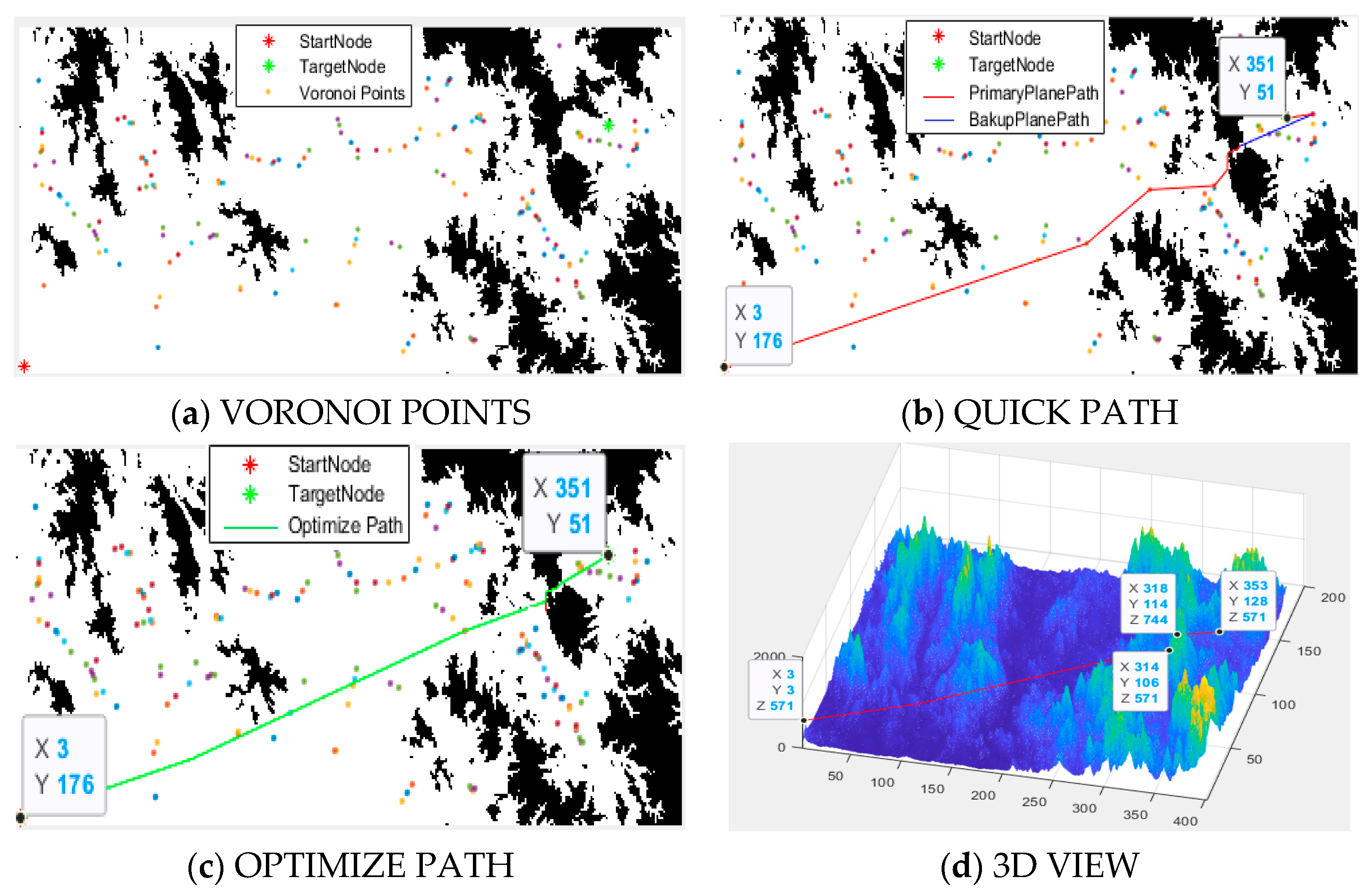
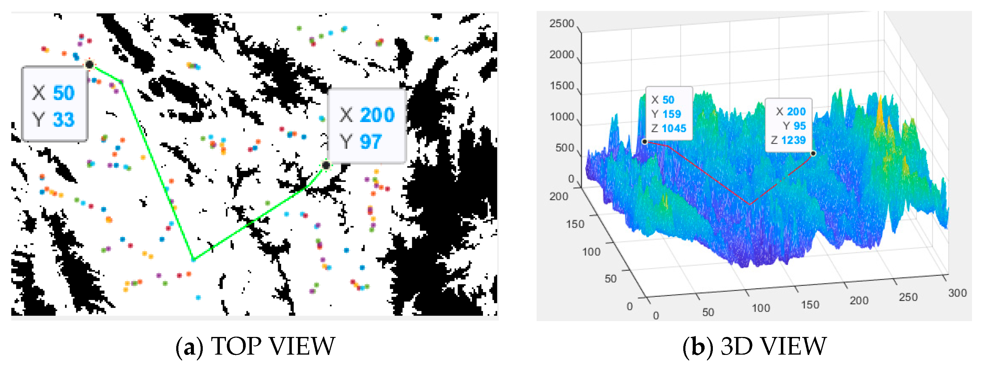
The planning path under the Voronoi–A* fusion algorithm simulation environment, as shown in Figure 1, features a UAV flight path with DEM cross-layer flights, enabling 3D obstacle traversal and successfully overcoming a mountain peak obstacle. This scenario’s planning process includes all steps, such as Voronoi vertex selection, A* search expansion, cross-layer flight, and interpolation optimization. 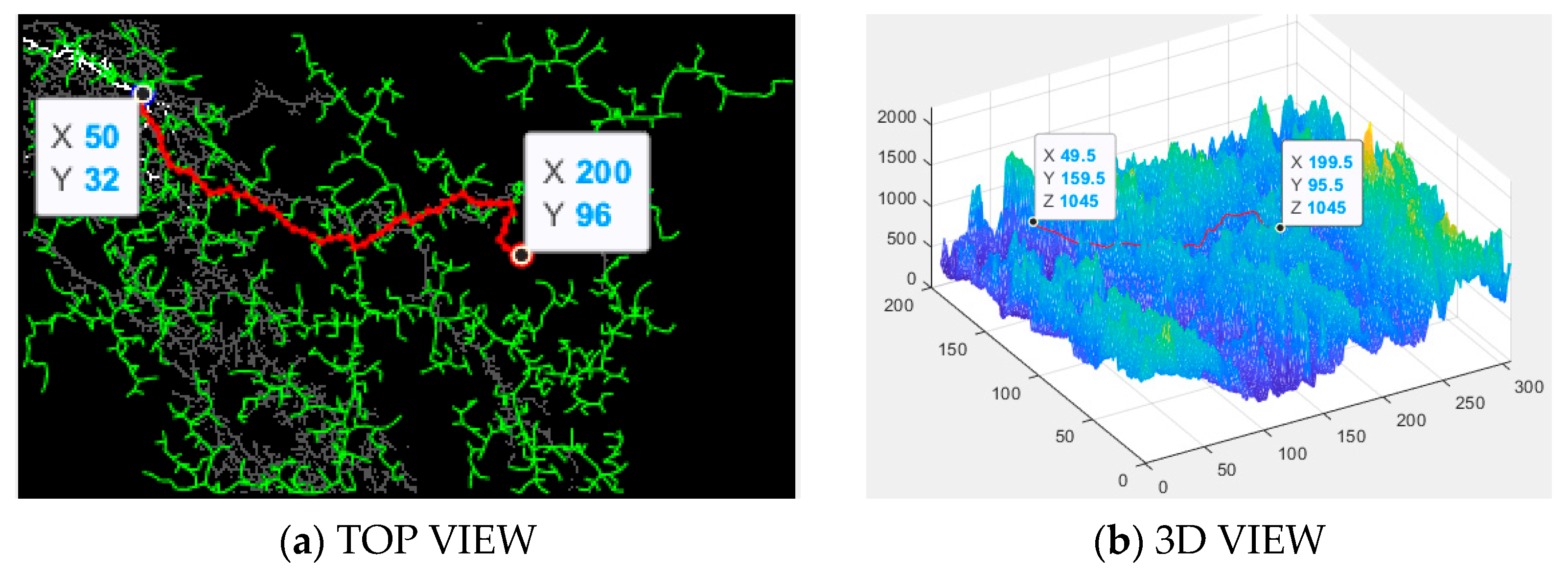Figure 7a illustrates the first step of the algorithm’s search for Voronoi vertices, while Figure 7b describes the algorithm’s rapid path search from the starting point to the endpoint. In this step, an A* expansion search is performed after crossing layers, resulting in the unoptimized search path. The blue line indicates a climb during this segment of the flight, the red * marks the start of the flight, and the green * marks the endpoint. 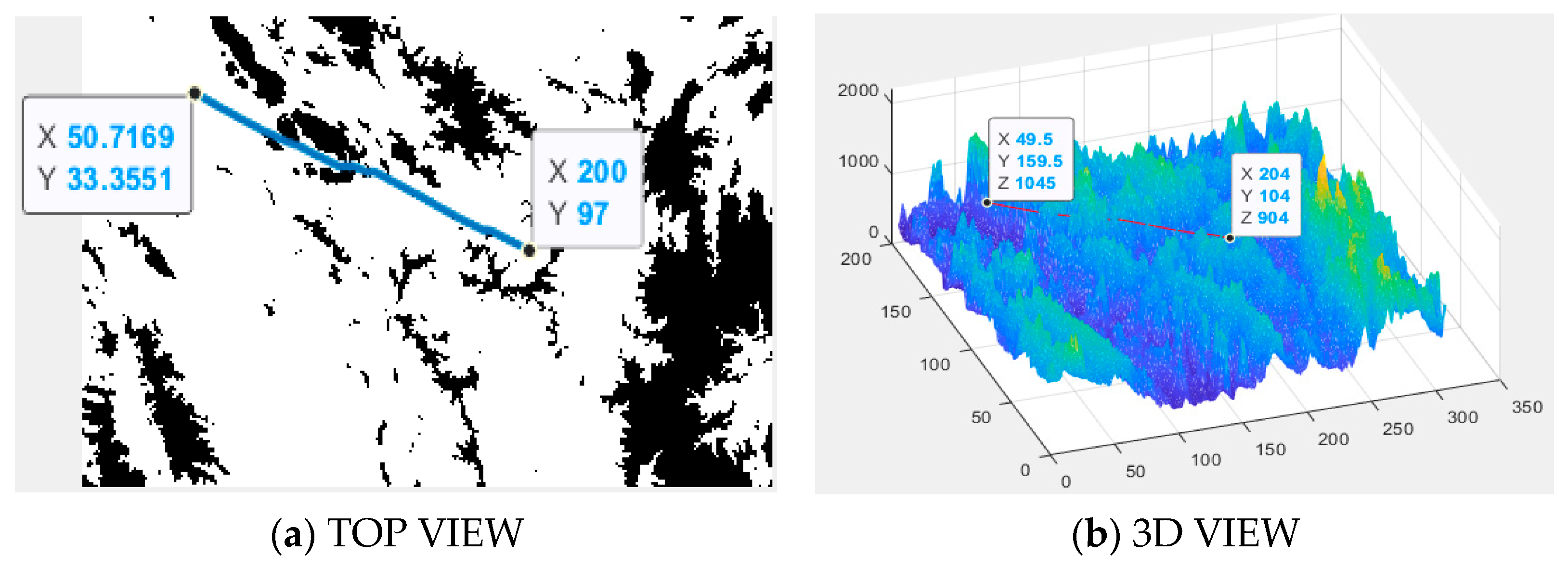Figure 7c shows the optimized flight path after interpolation optimization. 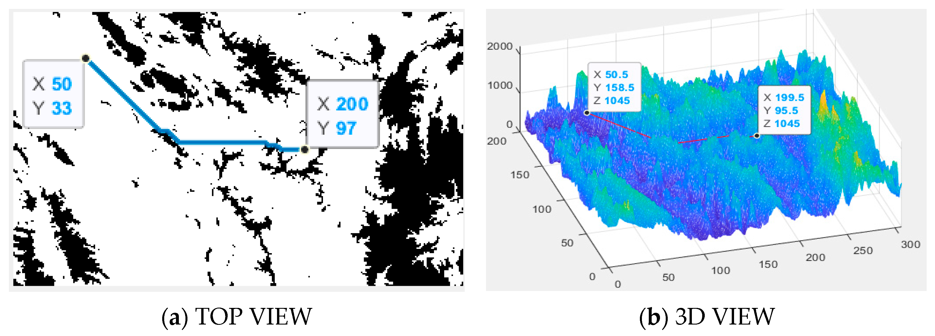Figure 7d presents the final 3D flight path.

(b)

The APF algorithm’s planned path in the simulation environment is shown in Figure 8, where the algorithm’s attraction coefficient is 15, the repulsion coefficient is 5, and the influence radius is 10 pixels. Due to the potential field balance issue in complex environments, it is clearly evident that the aircraft’s flight path directly passes through high mountains, resulting in a crash. Therefore, in terrains with complex topography and numerous three-dimensional obstacles, this method is not feasible.

(c)

The planned path of the RRT algorithm in the simulation environment is shown in Figure 9. Compared to the Voronoi–A* fusion algorithm, the path is noticeably more winding and complex. Additionally, due to the introduction of random factors, the consistency of the path planning is poor each time.

(d)

The planned path of the A* algorithm in the simulation environment is shown in Figure 10. It can be observed that the A* algorithm successfully plans a path that bypasses obstacles. In comparison to Figure 7, due to the influence of the A* search range, the number of planned path points increases, which results in higher computational complexity, longer calculation times, and a significantly longer total flight distance.

The test results of the four algorithms in this scenario, in addition to the start point (5, 177) and end point (351, 51), are compared, with statistics shown in

Table 2. Mountainous terrain test comparison chart.

Method	Collision	Number of Waypoints	Length (500 m)	Time (S)
Voronoi–A*	No	17	373.78	3.36 ± 1.67
A*	No	349	375.56	85.14 ± 12.21
APF	Yes	469	362.80	5.11 ± 1.3
RRT	No	143 ± 20	524.54 ± 77	99.21 ± 86.76

. ± represents the average value of the statistical results of 20 tests carried out for each algorithm.

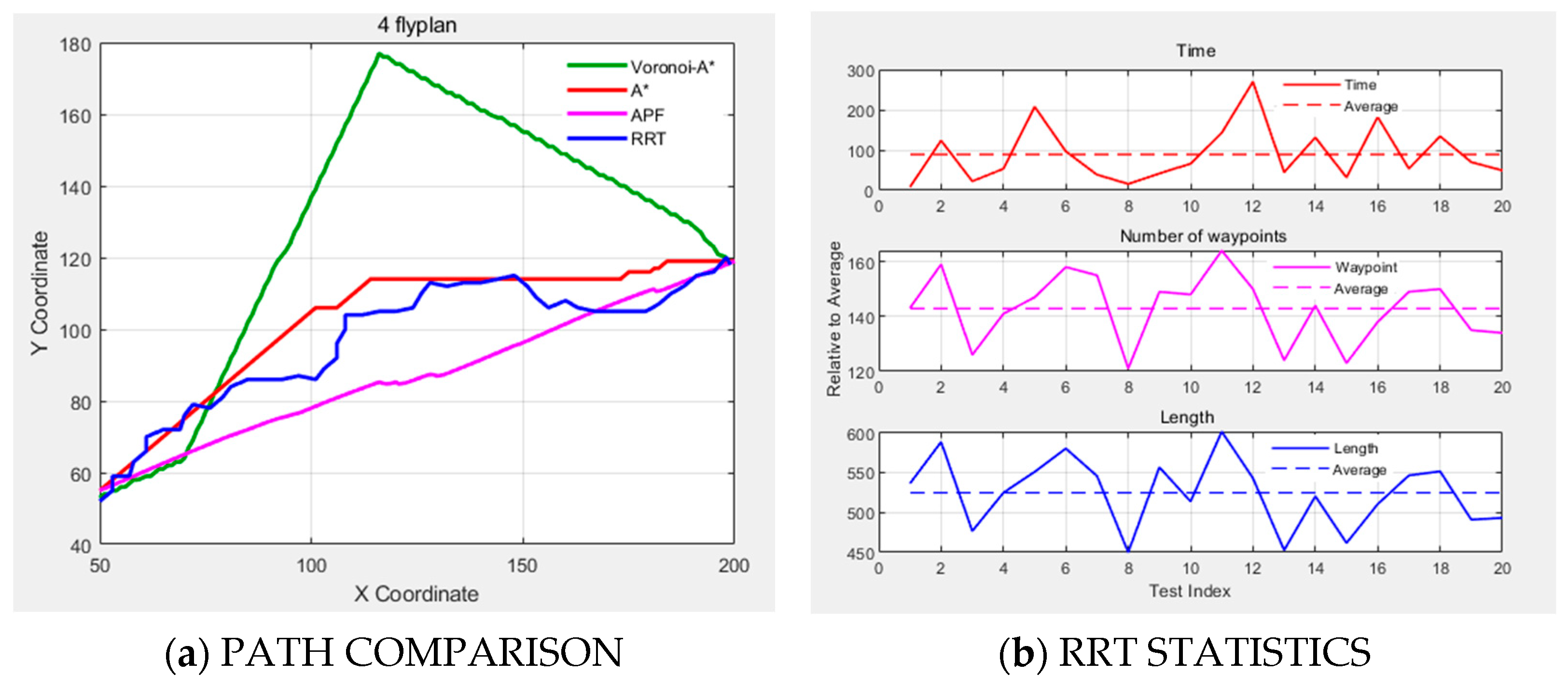
Figure 11a shows 2D simulation results, with four algorithms’ paths color-coded, while Figure 11b presents the statistical analysis results of 20 RRT trials, comparing time, waypoint count, and path length against their respective averages. The green line represents the self-developed Voronoi–A* fusion algorithm, the red line represents the A* algorithm, the magenta line represents the APF algorithm, and the blue line represents the RRT algorithm. The red * above the magenta line indicates the position where the obstacle was hit.

The simulation results of the mountainous terrain clearly show that the Voronoi–A* fusion algorithm has significant advantages in path planning. By combining Voronoi layering with A* search, inter-layer flights are enabled. The number of path points is only 4.9% of that of the A* algorithm (17 vs. 349), and the planning time is reduced by 96.1% (3.36 s vs. 85.14 s). This is the only method that fully implements three-dimensional obstacle avoidance.

Limitations of Traditional Algorithms: APF causes collisions with mountains due to the imbalance of the potential field; RRT has high path complexity and unstable path costs.

4.2. Scene 2: Hilly Terrain

The same starting and ending points are set with a map scale of 1:0.2. The simulation results of the four algorithms under this terrain are as follows.

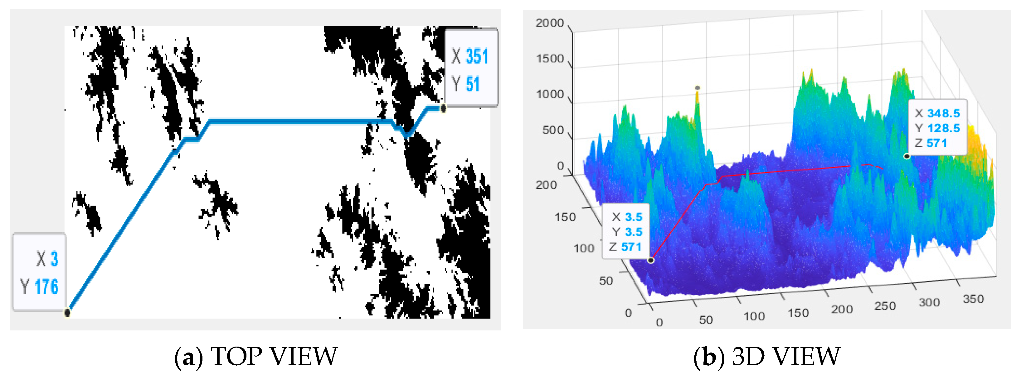
(a)

The planned path in the Voronoi–A* fusion algorithm simulation environment is shown in Figure 12. It can be observed that the aircraft’s flight path includes an alternate flight level after climbing, enabling it to cross mountainous terrain and successfully avoid obstacles.

(b)

The APF algorithm’s planned path in the simulation environment is shown in Figure 13. The algorithm sets initial parameters with a gravity coefficient of 15, a repulsion coefficient of 5, and an influence of 10 pixels. In a complex environment with mountainous terrain and numerous obstacles, it is clearly evident that the aircraft’s flight path directly passes through the mountains, causing the plane to crash. Moreover, the algorithm is sensitive to parameter settings. Therefore, the simulation results in this scenario indicate that the APF method is not feasible.

(c)

The RRT algorithm’s planned path in the simulation environment is shown in Figure 14. In comparison to the self-developed Voronoi–A* fusion algorithm, the path is noticeably more convoluted and complex. Moreover, across multiple simulation scenarios, the outcome of planning—success or failure—is uncertain. In cases of successful planning, the path is complex, and computational efficiency is relatively low.

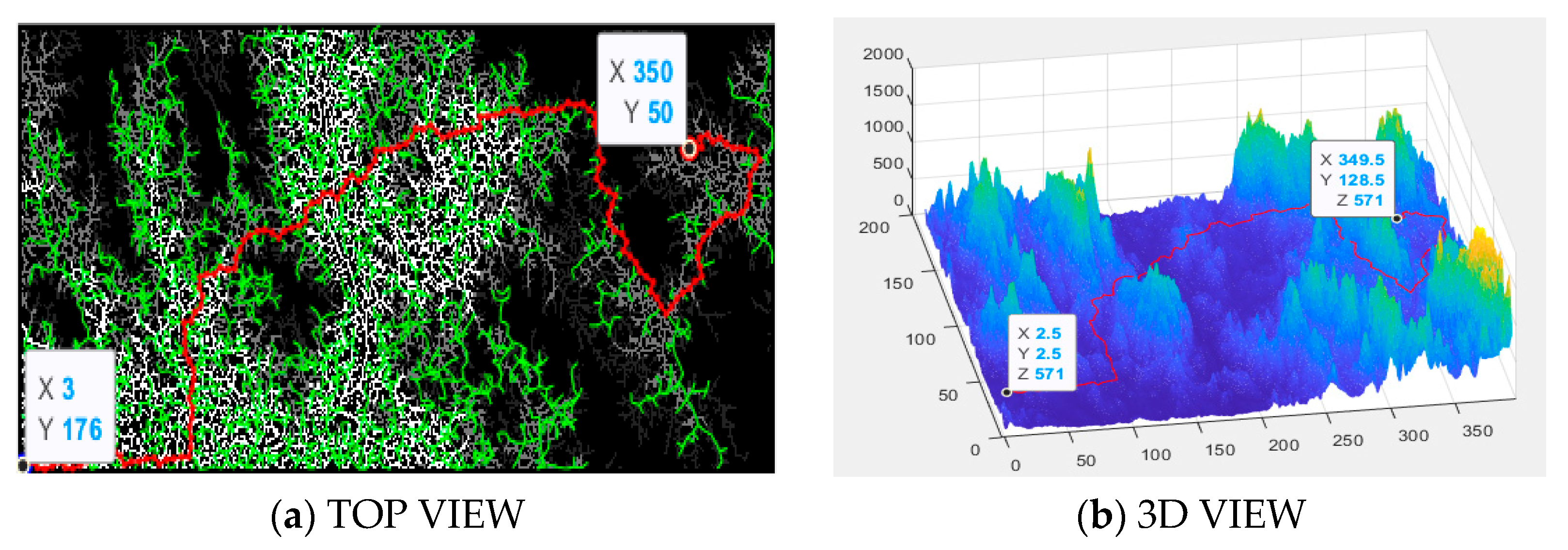
(d)

The planned path of the A* algorithm’s simulation environment is shown in Figure 15. In this scenario, the A* algorithm has an advantage over the Voronoi–A* fusion algorithm in terms of the total path length. However, the number of planned path points and the computation time are both inferior to those of the Voronoi–A* fusion algorithm. In practical engineering applications, in terrain with relatively more obstacles, the flight complexity of the A* algorithm increases.

The test results of the four algorithms in this scenario with start point (50, 55) and end point (200, 120) are compared, with statistical data shown in

Table 3. Hilly terrain test comparison chart.

Method	Collision	Number of Waypoints	Length (500 m)	Time (S)
Voronoi–A*	No	4	159.72	0.81 ± 0.18
A*	No	151	155.37	3.42 ± 3.22
APF	Yes	193	138.61	1.51 ± 1.16
RRT	No	62 ± 21	201.69 ± 23	75.96 ± 55.58

. ± represents the average value of the statistical results of the 20 tests carried out on each algorithm.

The 2D simulation planning path in this scenario is shown in Figure 16.

From the hilly terrain simulation results, it is evident that the path planning efficiency of the Voronoi–A* hybrid algorithm is significantly superior, with the number of path points being only 2.6% of that in the A* algorithm (4 vs. 151), and the planning time is reduced by 76.3% (0.81 s vs. 3.42 s). Additionally, the path length is nearly optimal (159.72 vs. 155.37). The failure of the APF is due to its sensitivity to parameters (gravitational coefficient of 15/repulsive coefficient of 5), which results in the flight path’s collision with obstacles, rendering it ineffective in a complex scenario.

4.3. Scene 3: Canyon Terrain

The same starting and ending points are set with a map scale of 1:0.2, and the test results of the four algorithms are as follows.

(a)

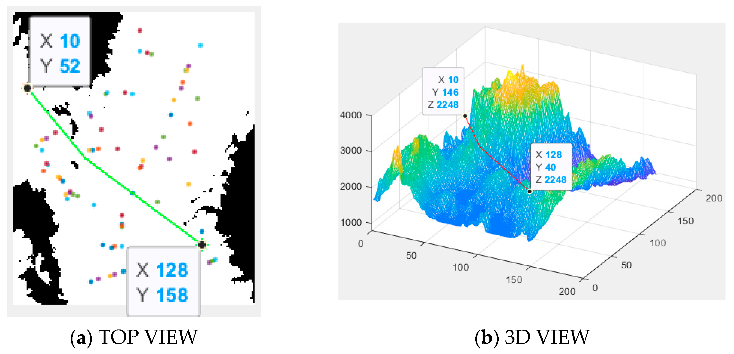
The planned path in the Voronoi–A* fusion algorithm simulation environment is shown in Figure 17. It can be observed that the aircraft only requires three key waypoints to successfully navigate over obstacles at the same flight altitude, realizing successful path planning.

(b)

The APF algorithm’s planned path in the simulation environment is shown in Figure 18. The parameter settings are consistent with those of the previous scene’s setup. As the middle portion of the canyon terrain is relatively open, the APF computes the gravitational field to guide obstacle avoidance. Path planning is successful. The planned path is short, and time costs are relatively low. Therefore, the APF algorithm is also applicable in certain open environments.

(c)

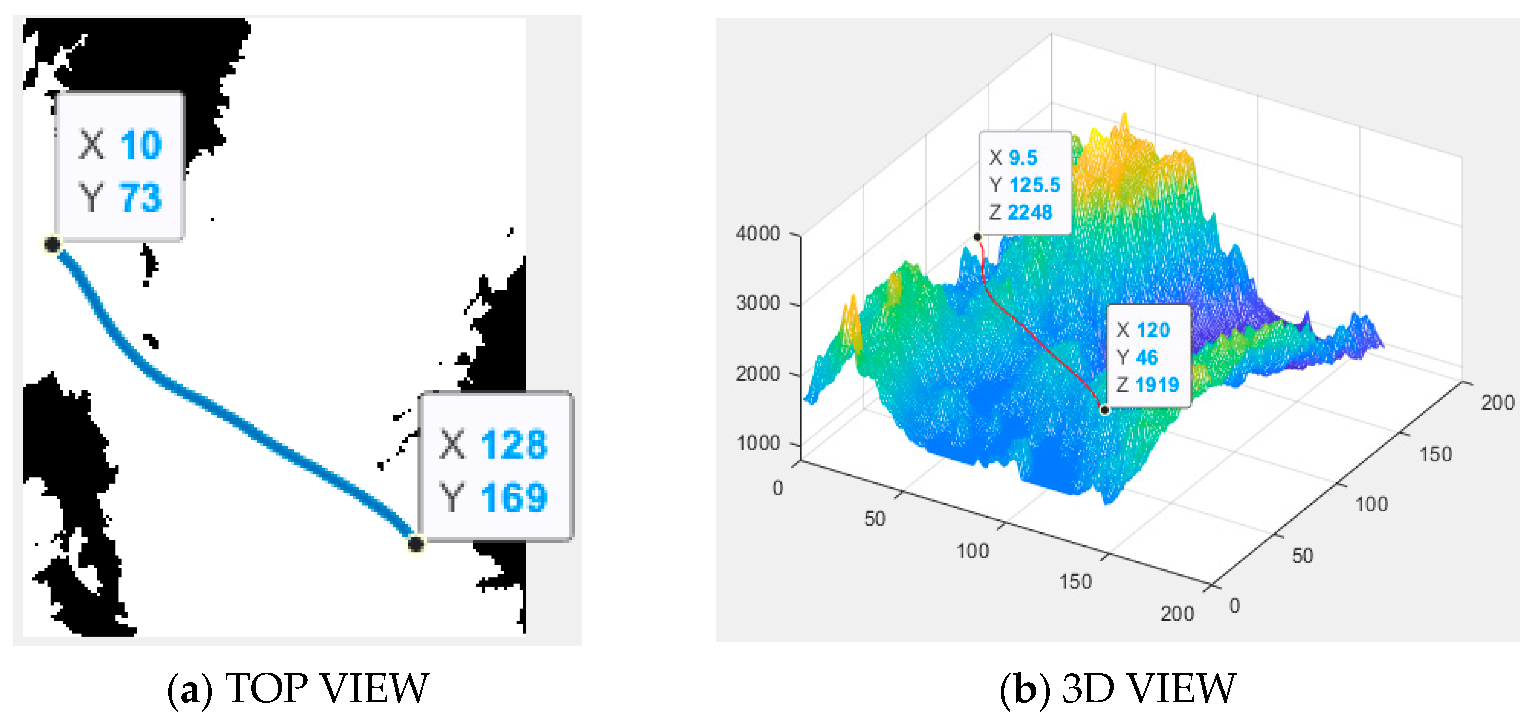
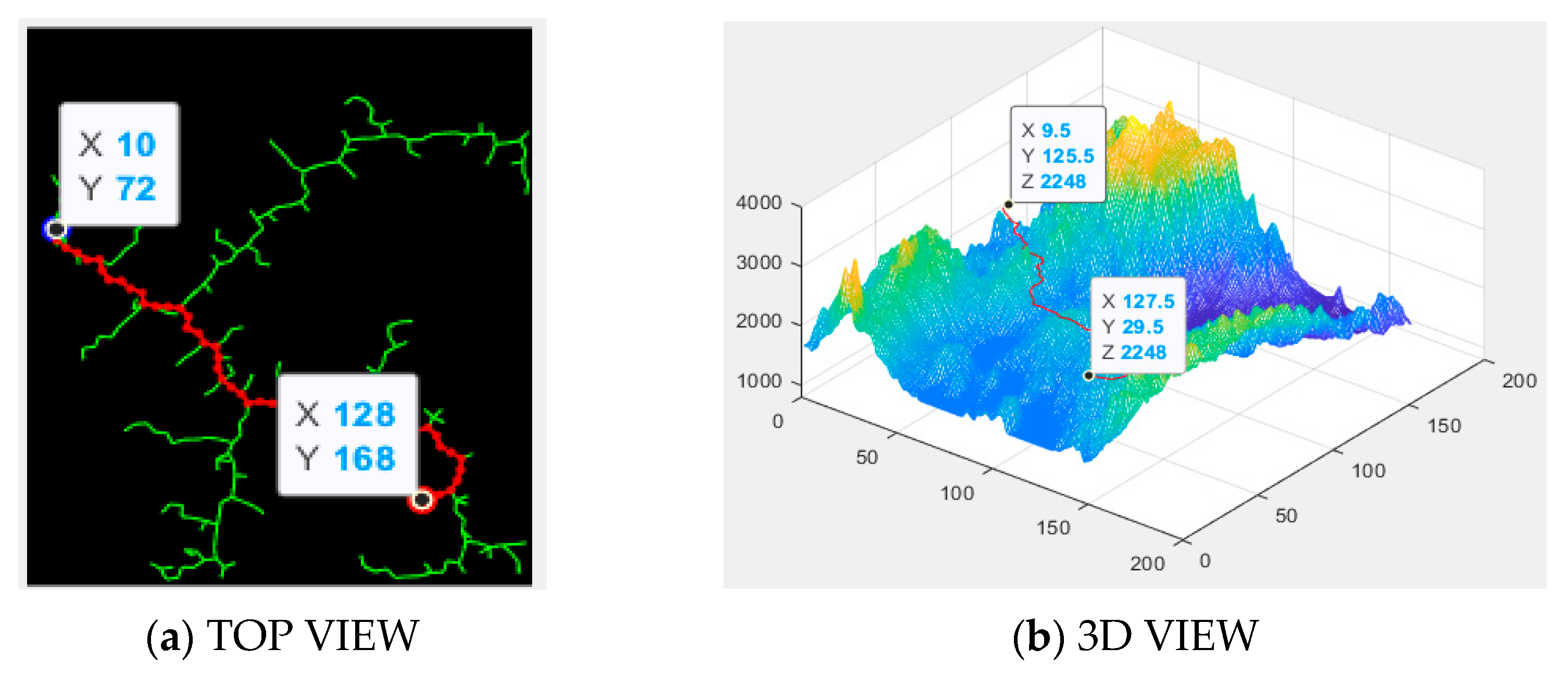
The path planning of the RRT algorithm in the simulation environment is shown in Figure 19. Compared to the Voronoi–A* fusion algorithm, the path is noticeably more winding and complex, resulting in higher computational complexity and longer computation times for real-world applications.

(d)

The planned path for the A* algorithm simulation environment is shown in Figure 20. The traditional A* algorithm can successfully navigate around obstacles. Compared to Figure 17, the number of planned path points increases, resulting in longer computation times.

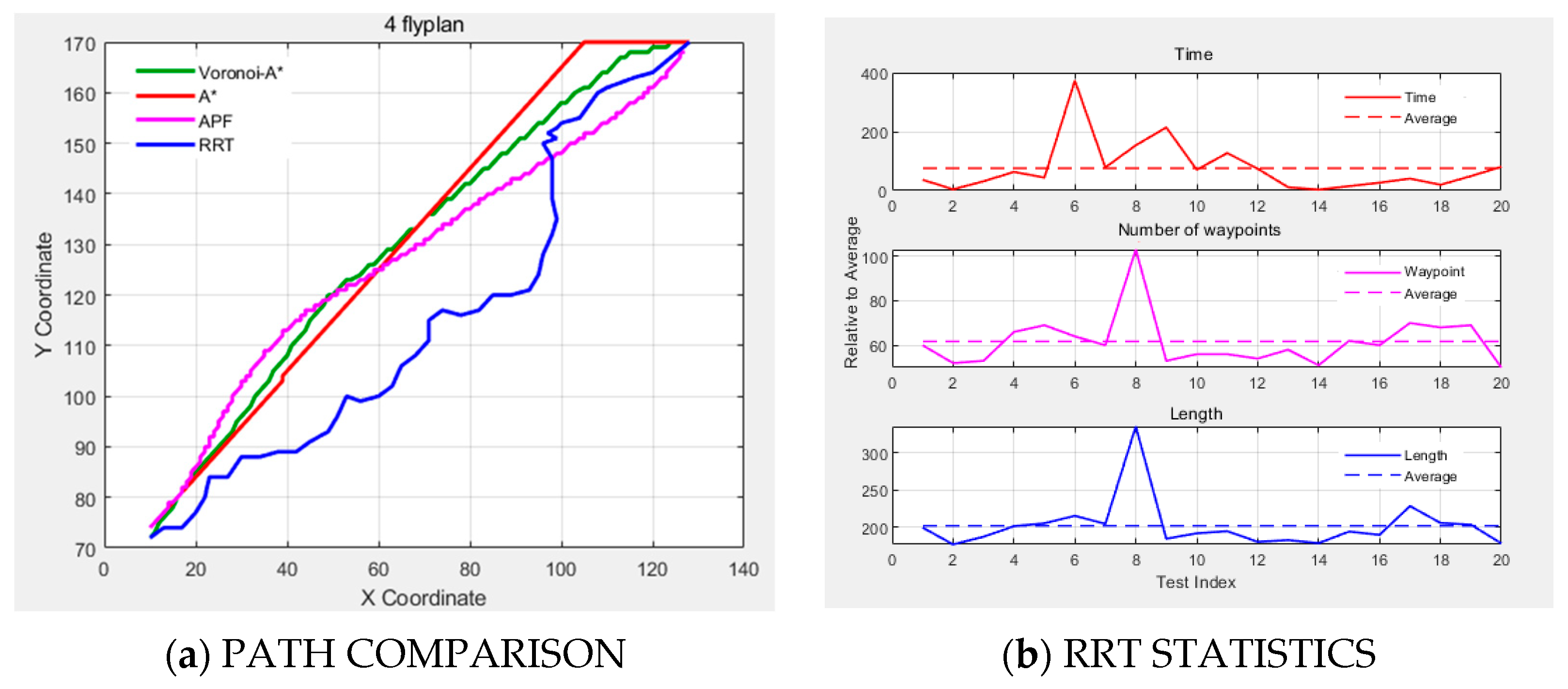
The test results of the four algorithms in this scenario with start point (10, 74) and end point (128, 170) are compared, with data summarized in

Table 4. Canyon terrain test comparison chart.

Method	Collision	Number of Waypoints	Length (500 m)	Time (S)
Voronoi–A*	No	3	132.12	0.81 ± 0.24
A*	No	120	134.28	3.64 ± 2.13
APF	No	190	139.54	2.41 ± 1.56
RRT	No	51 ± 11	164.46 ± 25	5.88 ± 3.47

. ± represents the average value of the statistical results of the 20 tests carried out on each algorithm.

The 2D simulation planning path in this scenario is shown in Figure 21.

From the simulation results of the canyon terrain, it can be observed that the Voronoi–A* fusion algorithm for path planning has the advantage of producing extremely simplified paths. Voronoi–A* enables horizontal obstacle avoidance using only three key points, and its planning time is 13.8% of that of the RRT algorithm (0.81 s vs. 5.88 ± 3.47 s), demonstrating its efficiency in open scenarios. The APF algorithm is sporadically applicable, successfully navigating only in canyon scenes with sparse obstacles, but the number of path points is 63 times greater than that of Voronoi–A* (190 vs. 3).

4.4. Analysis of Simulation Results in Multiple Scenarios

The comprehensive performance comparison of the simulation results across multiple scenarios is shown in

Table 5. Comprehensive performance comparison table (average).

	Voronoi–A*	A*	APF	RRT
Success of Planning	100%	100%	33%	96.7%
Average Number of Waypoints	8	207	284	85
Average Time (Seconds)	1.66	30.73	3.01	60.35

.

The summary in Table 5 indicates that the Voronoi–A* fusion algorithm significantly outperforms traditional algorithms in path planning performance within complex mountainous environments, as evidenced in the following aspects.

Path Planning Success Rate: The Voronoi–A* fusion algorithm successfully avoided obstacles and had no collisions in all test scenarios, while the APF algorithm failed to handle three-dimensional obstacles, resulting in crashes in mountainous and hilly terrain (success rate of only 33%). The RRT algorithm exhibited unstable performance, with planning failures occurring.

Path Efficiency:

(a)

Path Length: The Voronoi–A* path length is shorter than that of the traditional A* algorithm. For example, in mountainous terrain, the length is reduced by 0.5% (373.78 vs. 375.56 units), and in canyon terrain, it remains more efficient (132.12 vs. 134.28 units).

(b)

Number of Waypoints: The number of waypoints is reduced by an average of 92% compared to the A* algorithm (for example, in mountainous terrain, only 17 points are needed, whereas the A* algorithm requires 349 points), significantly reducing flight complexity.

Computational Efficiency:

The path planning time of Voronoi–A* is significantly superior to that of all the comparison algorithms:

(a)

Voronoi–A* has a faster average of 96.1% compared to the A* algorithm (e.g., in mountainous terrain, 3.36 s vs. 85.14 s).

(b)

It is 7.2 times faster than the RRT algorithm in canyon terrain (0.81 s vs. 5.88 ± 3.47 s).

(c)

The APF algorithm is fast (2.41 s) in open areas (such as canyons), but it completely fails in complex environments with dense obstacles.

Three-Dimensional Adaptability:

Voronoi–A* enables 3D obstacle avoidance through multi-layered flights, whereas APF and RRT only support 2D planning in certain scenarios. For example, in mountainous terrain, APF fails to cross peaks, causing the path to collide with obstacles, while Voronoi–A* successfully navigates around them in 3D.

In summary, the Voronoi–A* fusion algorithm, by combining the hierarchical strategy of Voronoi diagrams with the A* heuristic search, demonstrates significant advantages in path planning success rates, path optimality, computational efficiency, and three-dimensional obstacle avoidance. It provides an efficient and reliable solution for drone path planning in complex mountainous environments.

5. Conclusions

This study proposes a UAV trajectory planning method that is suitable for complex terrain. The method adopts a combined strategy comprising “Voronoi vertex-based quick trajectory generation + A* supplementary expansion of the trajectory.” Specifically, the algorithm first simplifies 3D route planning hierarchically using an adaptive DEM stratification strategy. Then, it uses the Voronoi vertex set within the flight plane as a sparse point network and employs a greedy heuristic search strategy for rapid trajectory planning, attempting to cross obstacles through backup planes. For obstacles that cannot be avoided, the traditional A* algorithm is used to locally connect 2D trajectories at the flight level. Finally, interpolation search is used to optimize the UAV’s flight trajectory. In the three specifically designed simulation scenarios, this combined algorithm significantly outperforms traditional single algorithms in terms of path planning success rates, computational efficiency, and adaptability to 3D terrain.

It should be noted that the Voronoi–A* fusion algorithm can quickly generate suitable and flyable paths by employing a global sparse search strategy via greedy optimization. However, this method exhibits the following three inherent limitations: (1) it cannot guarantee distance-optimal routes due to discrete DEM-based path planning, particularly in complex terrain; (2) its dependency on pre-existing DEM data restricts deployment in unmapped or dynamically changing environments; (3) the static environment assumption provides no inherent capability to handle unexpected obstacles such as complex weather conditions.

6. Future Research

Our preliminary validation in simulation environment has demonstrated the algorithm’s effectiveness, and our next step will involve deploying the proposed algorithm to ground control stations in order to command UAVs in mountainous terrain. Through the collection of real flight data, we will further validate the algorithm’s adaptability. Additionally, we plan to enhance global planning trajectories by integrating comprehensive environmental information from sensors and data links to advance research on dynamic obstacle avoidance algorithms. For instance, we will explore incorporating local-range mechanisms, such as the APF and Deep Q-Network (DQN), to enable dynamic obstacle avoidance and trajectory replanning. Furthermore, we aim to generalize the framework by modularizing the A* algorithm (used for route segment connection) and implementing it as one of several selectable algorithms (Dijkstra, PRM, APF, etc.). This modular approach will allow for combinatorial testing to improve applicability across diverse flight scenarios.