A Highly Robust Terrain-Aided Navigation Framework Based on an Improved Marine Predators Algorithm and Depth-First Search

Abstract

Autonomous underwater vehicles (AUVs) have obtained extensive application in the exploitation of marine resources. Terrain-aided navigation (TAN), as an accurate and reliable autonomous navigation method, is commonly used for AUV navigation. However, its accuracy degrades significantly in self-similar terrain features or measurement uncertainties. To overcome these challenges, we propose a novel terrain-aided navigation framework integrating an Improved Marine Predators Algorithm with Depth-First Search optimization (DFS-IMPA-TAN). This framework maintains positioning precision in partially self-similar terrains through two synergistic mechanisms: (1) IMPA-driven optimization based on the hunger-inspired adaptive exploitation to determine optimal trajectory transformations, cascaded with Kalman filtering for navigation state correction; (2) a Robust Tree (RT) hypothesis manager that maintains potential trajectory candidates in graph-structured memory, employing Depth-First Search for ambiguity resolution in feature matching. Experimental validation through simulations and in-vehicle testing demonstrates the framework’s distinctive advantages: (1) consistent terrain association in partially self-similar topographies; (2) inherent error resilience against ambiguous feature measurements; and (3) long-term navigation stability. In all experimental groups, the root mean squared error of the framework remained around 60 m. Under adverse conditions, its navigation accuracy improved by over 30% compared to other traditional batch processing TAN methods. Comparative analysis confirms superior performance over conventional methods under challenging conditions, establishing DFS-IMPA-TAN as a robust navigation solution for AUVs in complex underwater environments.

1. Introduction

Automated underwater vehicles (AUVs) play increasingly important roles in the exploitation of marine resources due to their high flexibility and autonomy. AUVs do not require a tether connection or inputs from an operator, enabling them to perform various complex underwater tasks in more challenging and harsh underwater environments [1]. With the advancement of AUV technology, they can now accommodate larger payloads and operate for longer durations [2]. These technological improvements have all driven the application of AUVs in marine resource development. To date, AUVs have been successfully applied in fields such as seabed mapping [3], polar exploration [4], marine biological research [5], and karst exploration [6].

To perform various complex underwater tasks, AUVs are typically equipped with multiple sensors including Inertial Navigation Systems (INSs), Doppler Velocity Logs (DVLs), and a Global Positioning System (GPS) [7]. Underwater navigation poses a significant challenge for AUVs because radio signals rapidly attenuate underwater, preventing them from utilizing GPS for navigation [8]. Additionally, Inertial Navigation Systems (INSs) cannot meet the long-term navigation requirements for AUV underwater operations due to accumulated errors.

Terrain-Aided Navigation (TAN) is an autonomous navigation method with no cumulative error that can effectively solve the underwater navigation problems faced by AUVs. TAN technology corrects the INS trajectory during navigation based on the measured terrain information to achieve accurate vehicle positioning. TAN can be divided into Terrain Matching Navigation (TMN) and the Simultaneous Localization and Mapping (SLAM) algorithms according to whether a prior terrain map is required [9]. The SLAM algorithm can realize navigation and localization without a prior map. In contrast, the TMN algorithm can achieve navigation by comparing the measured terrain information with the terrain information from a prior terrain map to correct the INS data. Filter-based methods and correlation-based batch processing methods are the two most classic categories of TMN algorithm. In recent years, a series of emerging terrain matching methods based on deep learning technologies have also been developed [10,11].

On the basis of this classification, TMN can further be divided into filter-based methods and correlation-based batch processing methods depending on the way in which the algorithm is implemented.

Filter-based methods use a variation of Bayesian filtering for recursion to achieve real-time correction of the AUV’s position. Bayesian filtering variations include the extended Kalman Filter (EKF), Particle Filter (PF), and Point Mass Filter (PMF) [12]. Among these, PF has been most widely studied due to its high precision. Zhou et al. [13] proposed the Kullback–Leibler Distance Particle Filter (KLD-PF), which can adjust the particle number according to its distribution in real time, thereby enhancing the efficiency of the PF. Zhou et al. [14] proposed the PF based on gradient fitting, which can select the appropriate distribution according to the terrain gradient characteristics and remove large gradient samples. Chai et al. [15] proposed a TAN method based on cubature PFs (CPF) that improves the PF performance by improving the particle resampling mechanism. Yousuf et al. [16] cascaded a fuzzy particle filter with the ESKF specifically to enhance the performance of TAN in highly nonlinear systems. Although the filter-based TAN method has excellent real-time and positioning accuracy, it often struggles to effectively correct when a large error occurs at a certain time. Therefore, how to improve the robustness of the algorithm has become a research focus of the filter TAN method. Liu et al. [17] integrated fuzzy logic into the PF to enhance the navigation robustness. Ma et al. [18] proposed a TAN method based on fuzzy theory that combined the grid PF and the contour PF to improve the effect of the PF in different terrains. The Rao–Blackwellized Particle Filter (RBPF) is an algorithm designed to address challenges in high-dimensional nonlinear problems. This enables adjustments of more physical quantities without compromising the real-time performance [19,20].

Numerous studies regarding the improvement and application of the RBPF algorithm have been conducted [21,22,23]. Zhang et al. [24] combined the maximum entropy criterion and adaptive filtering technology to improve the robustness of the algorithm based on the 3-D RBPF. Additionally, some studies have been conducted to correct the initial error in the PF algorithm [25,26,27].

The robustness of the PF algorithm remains insufficient in self-similar terrains or fuzzy measurements. Figure 1 shows that when terrains with similar heights exist in the search area, the estimated position of the PF will be misled.

Correlation-based batch processing TAN methods are, to a certain extent, less susceptible to interference from small-scale similar terrains. These methods often allow the AUV to travel for a period of time for recording the positions of the AUV indicated by the INS and terrain height of the points on the trajectory and find the most similar trajectory from the Digital Terrain Map (DTM) based on the correlation metric to correct the INS navigation data. The Terrain Contour Matching (TERCOM) algorithm, Iterated Closest Contour Point (ICCP), and the Particle Swarm Optimization (PSO) algorithm are the common correlation-based batch processing TAN systems.

TERCOM is a simple and effective TAN algorithm. However, its inability to correct heading angle error limits the system’s precision [28]. The ICCP algorithm finds the nearest reference point on the contour near the trajectory point and acquires the optimal transformation of the trajectory to the nearest reference point. Li et al. [29] integrated the ICCP algorithm matching results with the KF to enhance navigation accuracy and stability. Wang et al. [30] selected the paths of three data points in multi-beam data for parallel calculation to solve the problem of the large initial error divergence of the ICCP. Ding et al. [31] first used the maximum likelihood estimation for coarse matching based on multi-beam data and then used the ICCP algorithm for fine matching based on single-beam data. Zhang et al. [32] performed ICCP matching based on the terrain features obtained by the multi-beam data to address the issue of poor matching accuracy under large initial errors in the ICCP algorithm. The TAN method based on the PSO algorithm uses the parameters of the affine transformation model as optimization parameters to find the optimal transformation of the trajectory. Wang et al. [33] combined artificial bee colonies (ABCs) with PSO for terrain-assisted navigation.

As navigation corrections are periodic, not real-time, current batch-processing TAN methods using correlation are inferior to the PF algorithm in real-time performance and accuracy. In terms of robustness, the divergence induced by mismatches has a significant impact on the navigation stability of correlation-based batch processing TAN methods.

TAN methods based on optimization algorithms hold great potential according to their principles. This is because the final transformation found by the ICCP is contained within the search space of optimization-based TAN method. This indicates that when the performance of the optimization algorithm is sufficiently strong, the optimization-based TAN method is always capable of finding a solution with the same or better fitness than the ICCP method.

However, TAN methods based on optimization algorithms often struggle to achieve stable navigation performance under the influence of the terrains with similar height. These terrains with similar height are categorized into similar terrain and local optimum terrain. Specifically, the height of similar terrains exhibits the same or higher measurement correlation compared to the actual terrain. This renders such terrain impossible to distinguish using any correlation-based methods. As illustrated in Figure 2, when terrain height measurements fall at the lower bound of the error margin, point B matches the measurements better than the true terrain position. Local optimum terrain shows a slightly inferior correlation with measurements compared to the actual terrain. If the algorithm fails to explore the true terrain, this suboptimal solution may be selected, thereby disrupting the navigation process.

The concept of similar trajectories follows an analogous principle: they have superior comprehensive correlation across multiple points compared to the true trajectory. During terrain matching, there are typically a small number of similar trajectories and numerous local optimum trajectories. If the optimization algorithm inadequately explores the solution space, it may converge to a local optimum trajectory. Even if the algorithm finds the theoretical optimum, it cannot differentiate between similar trajectories and the true trajectory.

In response to the susceptibility of current TAN methods to self-similar terrains and fuzzy measurements, we propose a novel TAN framework based on an Improved Marine Predators Algorithm (IMPA) and Depth-First Search (DFS). This TAN framework outperforms various existing correlation-based batch processing TAN methods in navigation accuracy. In terms of navigation robustness, it is capable of self-correcting navigation divergence caused by self-similar terrains and fuzzy measurements, demonstrating exceptional adaptability. In this paper, our contributions are as follows:

(1) Existing optimization-based TAN methods are prone to being trapped in local optima, which often leads to mismatches during the navigation process. We attribute this issue to the insufficient performance of conventional intelligent optimization algorithms. To address this, we propose a novel Hunger Learning Algorithm using in the Marine Predators Algorithm (MPA) aiming to enhance information exchange among particles during the optimization process. Then, we apply the improved algorithm IMPA in the TAN framework. Simulation results demonstrate that the IMPA algorithm effectively avoids local optima and consistently locates the global optimum from the search areas. This significantly alleviates the issue of local optimum terrain interference encountered by optimization-based TAN methods. Furthermore, the matching results from the IMPA algorithm are integrated with a Kalman Filter (KF), enabling the system to operate in a real-time, periodically corrected mode. Based on this, IMPA-TAN provides higher navigation accuracy and stability for AUVs.

(2) Although the IMPA algorithm nearly eliminates the impact of local optima, it remains unable to distinguish self-similar terrains with a higher correlation due to terrain measurement errors during navigation. This adversely affects navigation accuracy and can even lead to divergence. To address this issue, this paper innovatively proposes a tree-structured framework based on Depth-First Search (DFS). During IMPA-TAN operation, this framework records all potential solutions within the bounds of measurement error. When subsequent navigation errors occur, it reverts to a previous navigation state and attempts alternative solutions for correction. Consequently, the proposed DFS-IMPA-TAN framework ensures stable navigation performance of the AUVs when encountering special conditions such as self-similar terrains and fuzzy measurements through node backtracking, which is difficult for other traditional TAN methods to achieve.

In this article, a novel TAN framework with strong robustness against self-similar terrains is proposed. Section 2 introduces the MPA optimization algorithm and its improvement. Section 3 introduces the IMPA-TAN and DFS-IMPA-TAN, including their principles and implementation details. Section 4 presents the simulation tests and in-vehicle experiments that validate the algorithm performance. Finally, Section 5 presents the conclusion.

2. MPA Algorithm and Its Improvement

2.1. Marine Predators Algorithm

The MPA is a metaheuristic algorithm inspired by marine predator hunting strategies. It studies the encounter rates between predators and prey under different velocity ratios using various random walk models. Based on these findings, the algorithm strategically selects the optimal movement pattern for predators and prey during different phases from two random walk models—Brownian motion and Lévy flight—to efficiently explore the search space. The specific generation procedures for Brownian motion and Lévy flight within MPA are detailed in reference [34].

The MPA algorithm initially defines two $n\times d$ matrices $x$ and $Elite$, where $n$ denotes the number of search agents and $d$ is the number of dimensions. The matrix $x$ contains the positions of all prey. Each row of matrix $x$ contains the current solution vector of one search agent. The matrix $Elite$ represents the predator, containing the optimal parameters found by the search agents. This Elite matrix is constructed by replicating the optimal solution, which is a $1\times d$ vector, $n$ times and stacking the copies vertically.

The MPA first generates a set of random solutions in the search space to achieve initialization. The initialization expression for the position of the i-th search agent $\overrightarrow{x_i}$ is given by Equation (1):

$$\overrightarrow{x_i}=\overrightarrow{LB}+\overrightarrow{r}\otimes (\overrightarrow{U\mathrm{B}}-\overrightarrow{LB}),$$

(1)

where $\overrightarrow{LB}$ and $\overrightarrow{UB}$ are the lower and upper boundaries of the search space, and $\overrightarrow{r}$ is a vector composed of random numbers from 0 to 1. The notation $\otimes$ represents entry-wise multiplications.

Then, the MPA enters its main loop. The total iterations $t_{\max }$ of this loop are equally divided into three stages. During the initial phase ($t\le {\displaystyle \frac{1}{3}}{t}_{\max }$), the optimal random movement strategies for prey and predators are Brownian motion and stillness, respectively. All search agents emulate prey behavior by performing random Brownian motion during this stage. The update process in this stage is modeled as follows:

$$\overrightarrow{ste{p}_i}=\overrightarrow{R_B}\otimes (\overrightarrow{Elit{e}_i}-\overrightarrow{R_B}\otimes \overrightarrow{x_i})\hspace{1em}i=1,2,\dots ,n,$$

(2)

$$\overrightarrow{x_i}=\overrightarrow{x_i}+P\cdot R\otimes \overrightarrow{ste{p}_i},$$

(3)

where $\overrightarrow{R_B}$ indicates random vector, which follows the Brownian movement. $P$ is a constant number that is set to 0.5 and $R$ is a random number between 0 and 1.

When ${\displaystyle \frac{1}{3}}{t}_{\max }<t\le {\displaystyle \frac{2}{3}}{t}_{\max }$, which is the second stage of MPA, the prey move in Lévy and predator moves in Brownian according to the optimal strategy, so as to realize exploration and exploitations. Half of the search agents will be assigned for exploration, and the other half will focus on exploitation in the phase. This phase is defined as follows:

$$\overrightarrow{ste{p}_i}=\overrightarrow{R_L}\otimes (\overrightarrow{Elit{e}_i}-\overrightarrow{R_L}\otimes \overrightarrow{x_i}) i=1,2,\dots ,n/2,$$

(4)

$$\overrightarrow{x_i}=\overrightarrow{x_i}+P\cdot R\otimes \overrightarrow{ste{p}_i},$$

(5)

$$\overrightarrow{ste{p}_i}=\overrightarrow{R_B}\otimes (\overrightarrow{R_B}\otimes \overrightarrow{Elit{e}_i}-\overrightarrow{x_i}) i=\mathrm{n} / 2,\dots ,n,$$

(6)

$$\overrightarrow{x_i}=\overrightarrow{Elit{e}_i}+P\cdot CF\otimes \overrightarrow{ste{p}_i},$$

(7)

$$CF={(1-{\displaystyle \frac{t}{t_{\max }}})}^{{\displaystyle \frac{2t}{t_{\max }}}},$$

(8)

where $\overrightarrow{R_L}$ is a random vector that indicates the Lévy movement, and $CF$ is the adaptive parameter to control the step size.

When $t\ge {\displaystyle \frac{2}{3}}{t}_{\max }$, which is the third stage of MPA, all search agents will act as the predator to moves in Lévy for exploitations according to the optimal strategy in this phase. The mathematical model of this phase is modeled as follows:

$$\overrightarrow{x_i}=\overrightarrow{R_L}\otimes (\overrightarrow{R_L}\otimes \overrightarrow{Elit{e}_i}-\overrightarrow{x_i}) i=1,2,\dots ,n,$$

(9)

$$\overrightarrow{x_i}=\overrightarrow{Elit{e}_i}+P\cdot CF\otimes \overrightarrow{ste{p}_i},$$

(10)

In addition, to prevent the MPA from falling into local optima, it simulates environmental issues such as the Eddy formation and FADs effect to make the search agent make longer jumps. The FADs effect is modeled as:

$$\overrightarrow{x_i}=\left\{\begin{array}{c}\overrightarrow{x_i}+CF[\overrightarrow{x_{\min }}+\overrightarrow{R}\otimes (\overrightarrow{x_{\max }}-\overrightarrow{x_{\min }})] \mathrm{r}\le \mathrm{FADs}\\ \overrightarrow{x_i}+[FADs(1-r)+r](\overrightarrow{x_{r_1}}-\overrightarrow{x_{r_2}}) \mathrm{r} > \mathrm{FADs}\end{array}\right.,$$

(11)

where $\mathrm{FAD}s$ is a constant number that is set to 0.2; and $r_1$ and $r_2$ are random numbers used to randomly select the vector in the matrix $x$.

After each change in the search agent’s position, the updated solutions of all search agents are compared with the stored solutions, and the superior ones are selected. The updated solutions of all search agents are also compared with the global optimum stored in the Elite matrix. Should it prove superior, the current solution replaces the global optimum. The Elite matrix is then updated by replicating this new global optimum solution n times.

2.2. Improved Marine Predators Algorithm

Although MPA can locate the optimal solution within the search space quickly and effectively, a single optimization method may also exhibit certain limitations. A novel hunger learning algorithm is proposed to enhance the utilization efficiency of search agents, thereby overcoming the problems of stacking at local optima.

Exchanging the information among particles is an effective method for enhancing optimization performance. It increases particle diversity and helps mitigate the risk of local optima. The proposed hunger learning algorithm in this paper draws inspiration from the Comprehensive Learning (CL) algorithm [35] and Hunger Games Search (HGS) algorithm [36]. It employs hunger values as a metric for population quality and encourages relative learning among search agents during the optimization process.

The hunger weight is a parameter used to weigh the performance of recent explorations of search agents. The expression of the i-th search agent’s hunger weight in the t-th iteration is as follows:

$$hungr{y}_t(i)=\left\{\begin{array}{c}hungr{y}_{t-1}(i)+{\displaystyle \frac{fit(i)-fi{t}_{best}}{fi{t}_{worst}-fi{t}_{best}}}\hspace{1em}fit(i)\ne fi{t}_{best}\\ 0\hspace{1em}\hspace{1em}\hspace{1em}\hspace{1em}\hspace{1em}\hspace{1em}\hspace{1em}\hspace{1em}\hspace{1em}\hspace{1em}\hspace{1em}fit(i)=fi{t}_{best}\end{array}\right.,$$

(12)

where $fit(i)$ is the fitness of the i -th search agent, and $fi{t}_{best}$ and $fi{t}_{worst}$ are the best fitness and worst fitness among all search agents, respectively. According to the expression, the search agent’s hunger value will accumulate if it exhibits an unsatisfactory exploration performance for several consecutive iterations; and the search agent’s hunger value will be reset to zero if it finds the global best value in the current iteration.

Search agents with high hunger values should learn from the search agents with lower hunger values to improve the search capability. In the hunger learning algorithm, agents are sorted in ascending order of hunger values; the latter half of the ranked agents learn from the former half. The learning target is defined as follows:

$$st(i)=\left\{\begin{array}{c} i\hspace{1em}\hspace{1em}\hspace{1em}\hspace{1em}\mathrm{rank}\left(\mathrm{i}\right)\le \mathrm{N}/2\\ N+1-i\hspace{1em}\mathrm{rank}\left(\mathrm{i}\right)>\mathrm{N}/2\end{array}\right.,$$

(13)

where $st(i)$ and $\mathrm{rank}(i)$ represent the learning target and the hunger value ranking of the i-th search agent, respectively. After completing the setting of the learning target, the learning coefficient is defined to represent the extent of learning from the target, as expressed by the following equation:

$$w(i)=a-{\displaystyle \frac{a}{1+e^{-5\frac{N+1-\mathrm{rank}(i)}{N}-b}}},$$

(14)

where $a$ is set to 0.6 and $b$ is set to 0.4 in this algorithm for making the search agent learn appropriately. Finally, the movement of the prey during the first and second stages of the original MPA algorithm is improved based on the learning target and learning coefficients as follows:

$$\overrightarrow{ste{p}_i}=\overrightarrow{R_B}\otimes (\overrightarrow{Elit{e}_i}-\overrightarrow{R_B}\otimes \overrightarrow{x_i}+w(i)*rand*(\overrightarrow{x_{st(i)}}-\overrightarrow{x_i})) i=1,2,\dots ,n,$$

(15)

$$\overrightarrow{ste{p}_i}=\overrightarrow{R_L}\otimes (\overrightarrow{Elit{e}_i}-\overrightarrow{R_L}\otimes \overrightarrow{x_i}+w(i)*rand*(\overrightarrow{x_{st(i)}}-\overrightarrow{x_i})) i=1,2,\dots ,n,$$

(16)

where $\overrightarrow{ste{p}_i}$ in (15) corresponds to the step size parameter in (2), and $\overrightarrow{ste{p}_i}$ in (16) corresponds to the step size parameter in Equation (4). In summary, the pseudo code of the IMPA is shown in Algorithm 1.

Algorithm 1: IMPA

Initialize the search agents using (1) While t < tmax do   Update Elite    For i = 1: n do     Update the hunger weight hungryt(i) using (12)     Update learning targets st(i) and learning coefficients w(i) using (13) and (14)   End for   If t ≤ tmax / 3     For i = 1: n do       Update xi using (15) and (3)     End for   Else if tmax / 3 < t ≤ 2tmax / 3     For i = 1: n / 2 do       Update xi using (16) and (5)     End for     For i = n / 2 + 1: n do       Update xi using (6)–(8)     End for   Else for i = 1: n do     Update xi using (9) and (10)   End for   Update Elite   Applying FADs effect and update xi using (11) End While

3. The Proposed DFS-IMPA-TAN Navigation Framework

3.1. IMPA-TAN Algorithm

The IMPA-TAN system provides navigation and positioning for AUVs based on INS, terrain measurement units, and DEM. The INS incorporates three vertically oriented gyroscopes and accelerometers, whose processed outputs yield angular and velocity increments per unit time. This information is further processed to calculate the AUV’s position, velocity, and attitude. The terrain measurement unit includes depth sensors and sonar bathymetry equipment, with its output continuously transmitted to the IMPA-TAN system for terrain matching and height damping correction. DEM should be stored in the system for terrain matching, whose resolution and accuracy both impact the final navigation performance.

TAN utilizes terrain height information for navigation, making terrain features a critical factor determining the final navigation performance. Before applying terrain-aided navigation, it is necessary to analyze the terrain features in advance and identify navigation-suitable areas. During operation, the AUV’s route should be planned to steer clear of unsuitable areas as much as possible to ensure navigation accuracy.

The IMPA-TAN is a method that uses the IMPA algorithm to find the optimal affine transformation of the INS trajectory to correct the navigation error. The IMPA-TAN method comprises three primary phases: the acquisition phase, the optimization phase and the correction process.

During the acquisition phase, the AUV performs the INS time update. Subsequently, it records the current position and measures terrain height at regular intervals based on the INS updates. After that, the system will correct navigation states based on multiple runs of the Kalman Filter (KF). These KF iterations share the same 15-dimensional state vector $x$, defined as follows:

$$x={[{\phi }_E,{\phi }_N,{\phi }_U,\delta v_E,\delta v_N,\delta v_U,\delta L,\delta \lambda ,\delta h,{\epsilon }_{bx},{\epsilon }_{by},{\epsilon }_{bz},{\nabla }_{bx},{\nabla }_{by},{\nabla }_{bz}]}^T,$$

(17)

where ${\phi }_E$, ${\phi }_N$, and ${\phi }_U$ represent the east, north, and vertical attitude errors, respectively; $\delta v_E$, $\delta v_N$, and $\delta v_U$ represent the east, north, and vertical velocity errors, respectively; $\delta L$, $\delta \lambda$, and $\delta h$ represent the longitude, latitude, and height errors, respectively; ${\epsilon }_{bx}$, ${\epsilon }_{by}$, and ${\epsilon }_{bz}$ represent the east, north, and vertical gyroscope biases, respectively; and ${\nabla }_{bx}$, ${\nabla }_{by}$, and ${\nabla }_{bz}$ represent the east, north, and vertical accelerometer biases, respectively.

After each INS update, the system will perform an update of the state vector using a discretized KF. The system state equation is as follows:

$$x_{t+1}=F_{t+1/t}{x}_t+{\eta }_t,$$

(18)

where $x_t$ represents the state vector at time $t$, and $F_{t+1/t}$ is the discretized one-step state transition matrix from time $t$ to $t$+1. ${\eta }_t$ represents the equivalent process noise, with its covariance matrix being $Q_t$. Following each acquisition of information from the terrain measurement unit of the AUV, the system first performs a measurement update of the KF based on the altitude to apply a dampening correction to the system. After completing the INS update and data collection of m data points, the system will enter the optimization phase.

After the acquisition phase, the system receives and saves the data from the IMU but pauses the INS time update. The INS update is resumed only after the optimization phase and correction process conclude, ensuring that subsequent updates proceed from the corrected navigation state.

The optimization phase is primarily based on the trajectory points and their corresponding terrain heights collected during the acquisition phase to optimize and solve. First, the system converts the coordinates of each trajectory point $(L_k,{\lambda }_k,h_k)$ into East–North–Up (ENU) coordinates $(X_k,Y_k,h_k)$ in meters to facilitate computation. It then seeks the optimal affine transformation for the INS-indicated trajectory, which maximizes the correlation between the transformed trajectory and the true terrain elevation. The expression for the affine transformation is as follows:

$$\left[\begin{array}{ccccc}{X}_1’& \dots & X_k’& \dots & X_m’\\ Y_1’& \dots & Y_k’& \dots & Y_m’\end{array}\right]=k\left[\begin{array}{cc}\cos \theta & \sin \theta \\ -\sin \theta & \cos \theta \end{array}\right]\left[\begin{array}{ccccc}{X}_1-X_0& \dots & X_k-X_0& \dots & X_m-X_0\\ Y_1-Y_0& \dots & Y_k-Y_0& \dots & Y_m-Y_0\end{array}\right]+\left[\begin{array}{c}dX\\ dY\end{array}\right]+\left[\begin{array}{c}{X}_0\\ Y_0\end{array}\right]$$

(19)

where $X_k’$ and $Y_k’$ represent the position of the $k$-th point after the transformation; $X_0$ and $Y_0$ record the position of the final point of the previous trajectory, or the starting point if it is the first match; $X_k$ and $Y_k$ denote the position of the $k$-th point of the INS indicated trajectory; and $[k,\theta ,dX,dY]$ represent the scaling factor, rotation angle, and the translation distance in the $X$-direction and in the $Y$-direction, which are the optimization parameters of the IMPA-TAN. The optimization fitness function is defined as follows:

$$fit={\displaystyle \frac{{\displaystyle \sum _{i=1}^m{(h_{mea,i}-h(X_i,Y_i))}^2}}{m}},$$

(20)

where $h_{mea,i}$ represents the measured height of the i-th point and $h(X_i,Y_i)$ represents the map terrain height of the i-th trajectory point after transformation.

After the optimization phase is completed, the system enters the correction phase. During this phase, the classical batch processing method directly corrects the position information based on the optimization results. However, there are two main problems: the first is that the update only adjusts the AUV’s position without correcting velocity and attitude information, which leading to errors in velocity and attitude that accumulate over time and causing trajectory deformation, thereby affecting subsequent data matching. The second is that the corrections are only made after a certain interval. This causes poor real-time performance.

To solve the problems of the IMPA-TAN in terms of error accumulation and real-time performance, we cascaded the position information of the optimal trajectory endpoint found by the IMPA algorithm with the INS update information using a KF filter. Both the velocity and attitude information could be corrected, and the real-time update was realized by outputting the INS information. In summary, the observation equation of KF is given as follows:

$$Z_t={[\delta {\tilde{L}}_t,\delta {\tilde{\lambda }}_t]}^T,$$

(21)

where $\delta {\tilde{L}}_t$ and $\delta {\tilde{\lambda }}_t$ represent the observed values of longitude and latitude, respectively. These values are obtained by subtracting the converted trajectory endpoint from the AUV’s current position. The discrete observation equation of the system is given as follows:

$$Z_t=H_t{x}_t+v_t,$$

(22)

where $H_t$ represents the observation matrix at time t, with a value of $[\begin{array}{ccc}{0}_{6\times 2}& I_{2\times 2}& 0_{7\times 2}\end{array}]$.$I_{2\times 2}$ is the identity matrix of size $2\times 2$. $0_{6\times 2}$ and $0_{7\times 2}$ are zero matrices of corresponding sizes, respectively. ${\nu }_t$ is the observation noise matrix, whose covariance matrix is $R_t$. The value of $R_t$ relates to the navigation accuracy of the IMPA-TAN algorithm. In this system, it is set to $diag{(\begin{array}{cc}50 \mathrm{m}/R_e& 50 \mathrm{m}/R_e\end{array})}^2$, where $diag$ denotes a diagonal matrix, 50 m is the estimated IMPA-TAN navigation accuracy, and $R_e$ is the Earth’s equatorial radius.

The IMPA-TAN algorithm complete flowchart is shown in Figure 3. Firstly, the IMU output provides the basic navigation information of the AUV. When the terrain measurement unit takes a measurement, the system utilizes KF for damping correction by incorporating navigation information and depth data.

At the same time, the system also records the position and terrain height of the current point. After the system acquires a certain number of points, it will find out the most probable trajectory through the IMPA algorithm according to the information of these points and the Digital Elevation Model (DEM). After that, the framework inputs the matching result into the KF to make feedback corrections to the position, velocity, and attitude.

Additionally, it should be noted that the frequencies of the two KF updates and the navigation information output are all different. The navigation information output is accompanied by INS updates that have the highest frequency. The first KF update occurs after the terrain measurement unit output, whose frequency is medium. The second KF update is performed after a certain number of points are collected by the terrain measurement unit and its frequency is the lowest.

The KF effectively corrects the navigation information when optimization results are sufficiently accurate, thereby maintaining stable and effective navigation. However, it also further extends the impact of incorrect optimization results. This not only produces a large positional error, but also causes the velocity and attitude to deviate from their true values, leading to subsequent trajectory deformation. However, the existence of the terrain measurement error determines the existence of similar solutions. Even if the IMPA algorithm accurately finds the transformation with the minimum fitness every time, a similar solution with lower fitness can still interfere with the navigation results. To address the issue of erroneous updates, a novel model was introduced that effectively mitigated their effects and enhanced navigation stability.

3.2. DFS-IMPA-TAN Framework

To correct the effect of similar solutions during the execution of the IMPA-TAN method, the robust tree model was proposed. Figure 4 shows the schematic of this model. In the schematic diagram, the AUV travels along the trajectory ‘1-3-4-6’. There are two similar trajectories, ‘1–2’ and ‘4–5’, in the map, and their terrain information is very similar to the real trajectory. When the measurement error is slightly larger, these trajectories may exhibit lower fitness values than the true trajectory, potentially causing them to be incorrectly selected as optimal by the IMPA-TAN algorithm. The robust tree is constructed as a tree structure to store all possible update results. If a deviation is detected during later steps, the algorithm reverts to the parent node; otherwise, it continues to follow the optimal solution. It essentially builds and maintains a tree database based on a DFS. As shown in Figure 4, if the first trajectory ‘1–2’ has lower fitness, the navigation updates, and the trajectory ‘1–3’ update results are simultaneously stored in the robust tree. During the second navigation update, if the deviation’s impact is minor and the IMPA algorithm successfully matches to trajectory ‘3–4’, the system continues to navigate. Conversely, if the deviation significantly affects the update and the IMPA algorithm is unable to identify a suitable affine transformation, the system returns to node 1. Subsequently, the system will access the node with the second lowest fitness, which stores the information for trajectories ‘1–3’, thereby continuing with accurate navigation updates.

According to the principles of robust tree and IMPA-TAN, there are many trajectories that are close to the real trajectories or similar trajectories during the optimization process. If all those trajectories are included in the robust tree, the system will be overwhelmed by the amount of computation introduced.

The parameter $R_t$ of KF in the IMPA-TAN algorithm defines the estimated error range of the optimization algorithm. If the estimated error values in the $X$ and $Y$ directions are both $R_p$, navigation will not be greatly impacted when the IMPA-TAN optimization result lies within a rectangular region around the real position with dimensions determined by $R_p$. According to this principle, the system will build robust trees by running IMPA twice.

The first IMPA is responsible for finding the global optimal transformation $[k_{op},{\theta }_{op},d{X}_{op},d{Y}_{op}]$ and then solving for the endpoint coordinates of the transformed trajectory:

$$\left[\begin{array}{c}{X}_{op,m}’\\ Y_{op,m}’\end{array}\right]=k_{op}\left[\begin{array}{cc}\cos {\theta }_{op}& \sin {\theta }_{op}\\ -\sin {\theta }_{op}& \cos {\theta }_{op}\end{array}\right]\left[\begin{array}{c}{X}_m-X_0\\ Y_m-Y_0\end{array}\right]+\left[\begin{array}{c}d{X}_{op}\\ d{Y}_{op}\end{array}\right]+\left[\begin{array}{c}{X}_0\\ Y_0\end{array}\right],$$

(23)

The second IMPA searches for all solutions with sufficiently low fitness during the optimization process. The specific solution process of the second IMPA is as follows: assuming the solution currently explored by IMPA is the i-th solution, with corresponding affine transformation parameters $[k_i,{\theta }_i,d{X}_i,d{Y}_i]$. Its fitness is first calculated according to Equations (19) and (20). Then, the following formula is used to determine whether the current solution satisfies the fitness condition:

$$fi{t}_i\le fitm,$$

(24)

where $fi{t}_i$ denotes the fitness value of the i-th solution, and $fitm$ is the maximum tolerable fitness value in the robust tree. In this system, if the terrain elevation measurement error satisfies ${\nu }_h\sim N(0,{\sigma }_h)$, then $fitm=2{\sigma }_h^2$. Subsequently, for solutions satisfying the fitness condition, it is necessary to find the grid coordinates of their endpoints. Substituting $[k_{op},{\theta }_{op},d{X}_{op},d{Y}_{op}]$ in Equation (23) in place of $[k_i,{\theta }_i,d{X}_i,d{Y}_i]$ yields the trajectory endpoint coordinates $[X_{i,m}’,Y_{i,m}’]$. Following this, the grid coordinates corresponding to this solution are calculated as follows:

$$\left[\begin{array}{c}Xc\\ Yc\end{array}\right]=\left[\begin{array}{c}trunc((X_{i,m}’-X_{op,m}’)/R_p)\\ trunc((Y_{i,m}’-Y_{op,m}’)/R_p)\end{array}\right],$$

(25)

where $[X_c,Y_c]$ represents the obtained grid coordinates, and $trunc( )$ denotes the function that truncates the fractional part. After determining the grid coordinates of the current solution, the storage status within the current grid cell is first checked. If the current solution’s grid does not contain any other solutions, the relevant information of the current solution will be recorded. Otherwise, the grid records the solution with the lower fitness value. After storing a new solution, nodes will be sorted by fitness value to prioritize lower-fitness solutions in subsequent exploration. Figure 5 shows the schematic of robust tree construction where P1 to P6 are six possible trajectory transformations, and the index number corresponds to their fitness ranking. Based on the robust tree construction method, there are only three child nodes in this update. In addition, according to the principle of the robust tree, the end point of the true trajectory will be within the area covered by three nodes.

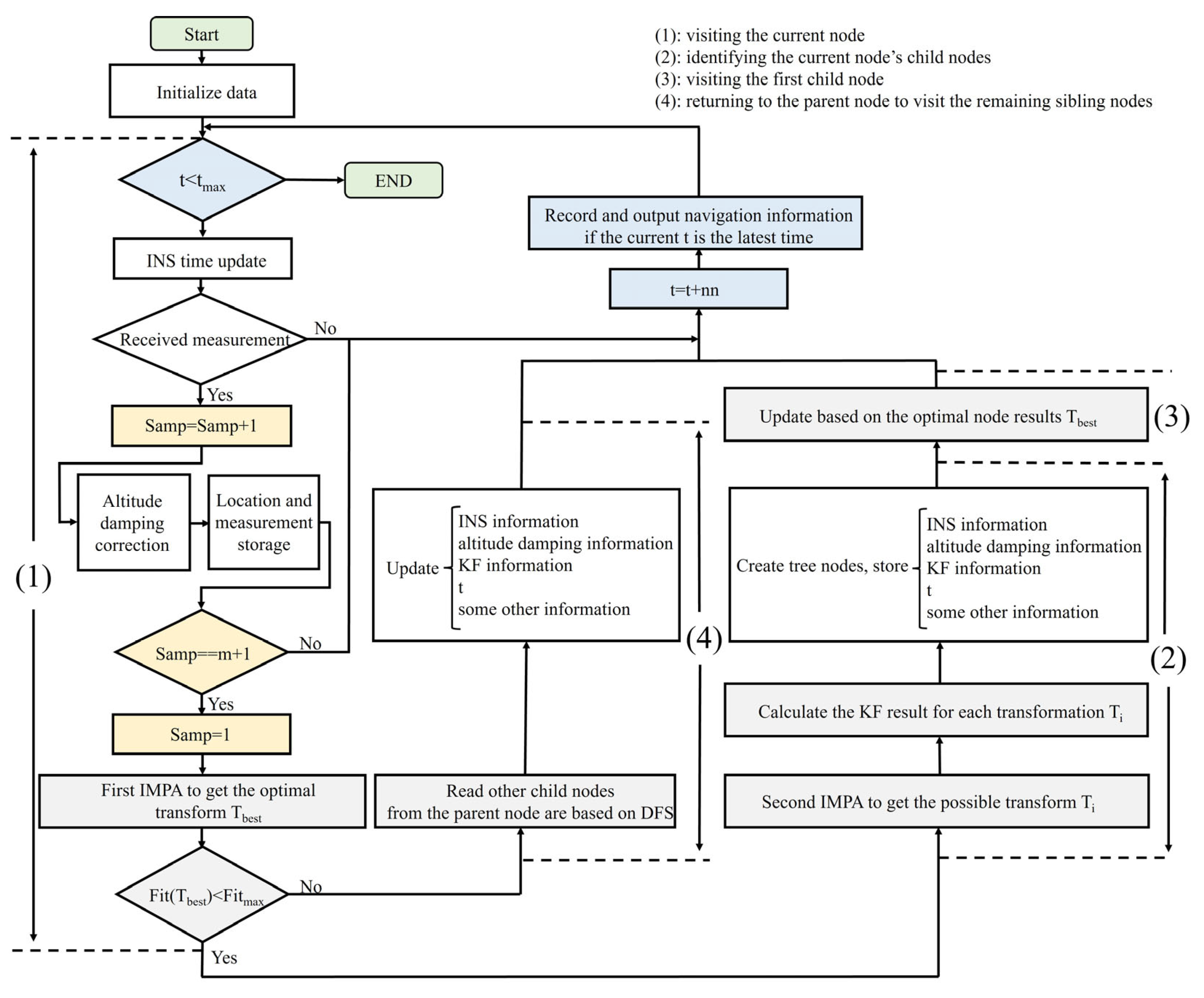
The primary flow of the DFS-IMPA-TAN framework is shown in Figure 6. The loop’s body corresponds to four phases of DFS: visiting the current node, identifying the current node’s child nodes, visiting the first child node, and returning to the parent node to visit the remaining sibling nodes. Each phase is clearly labeled in the flowchart.

During the first phase of the DFS process, corresponding to the ‘visiting the current node’ step, the system performs a series of operations that include INS updates, altitude damping and the first IMPA optimization. $t_{\max }$ is the navigation duration. In playback experiments, it is set to the final moment of navigation; while in actual applications, the loop only exits upon manual termination. The visit result of the node depends on the fitness of the first IMPA’s optimal solution. If the fitness is too high, the node is rejected.

The second and third stages correspond to ‘identifying the current node’s child nodes’ and ‘visiting the first child node’, respectively. During the second stage, the second IMPA is utilized to construct the robust tree. For each child node, the KF update results are calculated and stored along with time and other parameters. It is essential to ensure that all relevant parameters are recorded for reproducing the navigation state at any given time. The contents saved in the i-th node are as follows:

$$tree(i)=\{INS,KF,ALT,[X_0,Y_0],t\},$$

(26)

where INS represents variables related to inertial navigation; KF denotes variables related to the Kalman Filter; ALT signifies variables related to altitude damping; $[X_0,Y_0]$ is the endpoint of the node at the previous time step, and t contains all the variables used for recording time.

During the third stage, the system inputs the parameters of the first child node into the system to continue updating.

The fourth corresponds to the ‘returning to the parent node to visit the remaining sibling nodes’ step. The system will revert to previous time nodes to perform updates and correct the prior erroneously updated results. Navigation information is output only when the current time t is the latest moment.

Finally, it is worth noting that the tree needs to be pruned during system operation to prevent excessive memory consumption by stored data. The method used in this framework only keeps the nodes of the newest 10-level tree in order to conserve computing and storage resources without affecting the performance of the robust tree.

In Section 3, we designed the DFS-IMPA-TAN framework. Compared with traditional TAN algorithms, this framework can better deal with the problems of terrain with self-similar features or fuzzy measurements and maintains real-time, accurate, and stable navigation.

4. Simulation and Experimentation

4.1. Simulation Test

To validate the accuracy and robustness of the navigation method, simulations were conducted based on the DEM map of a real seabed, as shown in Figure 7, that was released by the United Kingdom Polar Data Centre [37]. This DEM was compiled from multibeam echosounder data collected by multiple vessels within the selected areas within the Orkney Passage, Scotia Sea.

4.1.1. Simulation Test I: Navigation Accuracy Test

First, the performance of the DFS-IMPA-TAN method was compared with other algorithms under ideal terrain conditions. Areas with high speed, low measurement error, and the most pronounced terrain variations were selected for the simulation test. The specific parameters of the simulation test are shown in

Table 1. Parameter settings for simulation test I.

Category	Parameter	Value
IMU	Gyroscope bias	0.008°/h
	Accelerometer bias	50 μg
	Gyroscope random error	$0.002°/\sqrt{\mathrm{h}}$
	Accelerometer random error	$10 \mathsf{\mu }\mathrm{g}/\sqrt{\mathrm{h}}$
	Output frequency	200 Hz
Terrain Measurement Unit	Height measurement error	N(0 m, 3 m2)
	Output frequency	1 Hz
AUV	Speed	10 m/s
	Initial attitude error	[0.5, 0.5, 1]°
	Initial velocity error	[0.1, 0.1, 0.1] m/s
	Initial position error	[10, 10, 10] m
DEM	Grid size	50 m × 50 m

.

Table 2. Comparative experiment simulation parameter settings for simulation test I.

Category	Parameter	Value
ICCP	Intervals	6 s
	Number of sampling points	15
PF	Number of particles	1000
	Resampling threshold	2/3 N
	Process noise covariance	diag [6 m2, 6 m2]
TERCOM	Number of sampling points	130
DFS-IMPA-TAN	Number of sampling points	130

lists the core parameters of the comparative algorithms. For the ICCP algorithm, the core parameters include the intervals and number of sampling points. Multiple combinations were tested in this study, with parameters adopted from Ding et al. [31]. For the PF, the number of particles was set to 1000 and the resampling threshold was configured at two-thirds of the number of particles, which was a conventional setting. The process noise covariance was tested across a range of values, with optimal parameters selected for this study. Specifically, in the Simulation Test I and II, it was set to diag [6 m², 6 m²]; while in the in-vehicle experiment, it was set to diag [3 m², 3 m²].

The results of simulation test I are shown in Figure 8 and Figure 9. In addition, the maximum errors and root mean squared error (RMSE) are shown in

Table 3. Maximum values and RMSE of the navigation errors for different algorithms in simulation test I.

Method	Maximum Error (m)	RMSE (m)
PF	115.85	37.98
DFS-IMPA-TAN	146.46	52.31
ICCP	333.34	131.5
TERCOM	898.46	357.9
INS	1826.2	1262

. The equation for RMSE is as follows:

$$RMSE=\sqrt{{\displaystyle \frac{1}{T}}{\displaystyle \sum _{k=1}^T{(x_k-{\widehat{x}}_k)}^2}},$$

(27)

where $T$ represents the navigation time, and $x_k$ and ${\widehat{x}}_k$ are the true position and predicted position at time $k$, respectively. Simulation parameters for the comparative experiments are set as follows:

According to the simulation results, it was found that the navigation accuracy of DFS-IMPA-TAN is slightly lower than that of the PF under the suitable conditions. This result can be attributed to a characteristic of the batch processing method: its periodic correction of navigation information rather than real-time correction. This work characteristic limits the precision of DFS-IMPA-TAN. However, owing to the powerful optimization capability of the IMPA algorithm, the transformations it found were closer to the real trajectories. Therefore, its navigation accuracy was significantly better than those of ICCP and TERCOM algorithms, which are also batch processing methods.

4.1.2. Simulation Test II: Navigation Robustness Testing

Most of the current TAN algorithms have high requirements for terrain and measurement accuracy. Algorithms such as PF tend to diverge easily when they encounter situations such as self-similar terrain features or measurement uncertainties. This makes it difficult to maintain the navigation stability of the AUVs in harsh environments. However, the DFS-IMPA-TAN has better robustness to these situations due to the assistance of the robust tree.

To test the robustness of the proposed method, a simulation test with approximately 25 h of travel was conducted, at a speed of 5 m/s and a height measurement variance of 5 m². Due to significant measurement errors and more arbitrary path selection approaches, the existing TAN methods struggle to maintain satisfactory navigation performance.

Figure 10 depicts the performance of different algorithms during the initial segment of the navigation trajectory. It can be observed that the PF algorithm exhibits divergence after maintaining high-precision navigation for a certain distance. This occurs because certain terrains along the navigation path induce localization deviations in the PF. Once the PF’s trajectory deviates from the ground truth, it struggles to autonomously recover, eventually leading to navigation divergence. Both the TERCOM and ICCP algorithms also fail to sustain accurate navigation. In contrast, the DFS-IMPA-TAN maintains stable operation under these adverse conditions.

The simulation results of DFS-IMPA-TAN are shown in Figure 11 and Figure 12. The results showed that the DFS-IMPA-TAN framework remained stable throughout the navigation process that covered most of the maps, and this was difficult to achieve using the other current TAN methods.

The RMSE of simulation test II was 62.81 m and the maximum error was 464.99 m. These results verified the proposed method’s robustness. According to the simulation result, more areas will be included in the terrain navigation area based on the framework.

Furthermore, to validate the real-time performance of the algorithm, during its execution, the system records the current time whenever the robust tree advances to the next layer. Upon completion of the entire simulation, differences are computed from the recorded time series. This establishes the time required to process a single trajectory segment. This duration encompasses the entire process, including INS update, IMPA matching, and robust tree computation. The differential results are plotted in Figure 13.

From Figure 13, it can be observed that navigation divergence of the AUV occurred only during the initial phase of the navigation process. To address this divergence, the system performed 1–2 layers of backtracking, resolving the issue in approximately 8 s. Under normal conditions without divergence, the system completes the full computational process in about 3 s. In this simulation, the system was configured to perform matching and updating only after recording every 130 trajectory points, equivalent to a 130-s interval. In view of the computation time per cycle being significantly shorter than the update interval, the system can maintain continuous real-time operation in practical applications.

4.1.3. Simulation Test III: Navigation Robustness Testing

To check the performance of the optimization algorithm, the classic benchmark CEC-2017 is used for testing. F1–F6 in the CEC-2017 benchmark are single-peak functions used to test the convergence ability of an algorithm, whereas F7–F13 are multi-peak functions used to evaluate the exploration ability of an algorithm.

In simulation test III, the parameters for the optimization algorithms PSO and F-WAPSO were set according to reference [33]. The optimization algorithm ABC was the standard artificial bee colony algorithm, implemented as described in reference [38]. It is worth noting that the optimization algorithm used in reference [33] employed 100 particles over 100 iterations, while the MPA algorithm typically uses 30 particles over 500 iterations. To ensure the rigor of the simulation test, the PSO and F-WAPSO algorithms were calculated using two configurations: 30 particles for 500 iterations and 100 particles for 150 iterations, and the superior optimization results were selected.

Simulation experiments were conducted by applying each optimization algorithm to each function for 50 independent optimization runs, and the mean value of the results was calculated. The results are shown in

Table 4. Optimization-seeking averages of different optimization algorithms for different functions.

Method	IMPA	MPA	F-WAPSO	ABC	PSO	Optimum
F1	2.88 × 10−23	9.89 × 10−22	4.57 × 10−1	3.84 × 10	5.63 × 10	IMPA
F2	1.87 × 10−13	1.65 × 10−11	6.13	1.75 × 10	6.37 × 102	IMPA
F3	2.82 × 10−2	1.63 × 10−2	5.31 × 103	6.76 × 104	1.02 × 104	IMPA
F4	3.66 × 10−12	2.76 × 10−8	1.53 × 10	8.16 × 10	1.90 × 10	IMPA
F5	4.63 × 10	4.65 × 10	3.21 × 102	1.13 × 105	3.02 × 104	IMPA
F6	1.30 × 10−1	2.22 × 10−1	7.65 × 10−1	3.50 × 10	4.64 × 10	IMPA
F7	2.06 × 10−3	1.67 × 10−3	1.09	1.64 × 102	6.02	MPA
F8	−1.38 × 104	−1.36 × 104	−1.39 × 104	−1.74 × 104	−1.23 × 104	ABC
F9	0	0	2.02 × 102	3.19 × 102	4.51 × 102	IMPA&MPA
F10	3.06 × 10−13	4.25 × 10−11	2.23	1.31 × 10	9.95	IMPA
F11	0	0	1.22	9.28 × 10	3.67	IMPA&MPA
F12	3.80 × 10−2	4.61 × 10−2	1.15	4.97 × 106	5.47 × 103	IMPA
F13	7.36	7.72	8.55	1.84 × 107	3.13 × 105	IMPA

. According to the results, the IMPA algorithm performed better than the MPA algorithm on most functions and significantly outperformed other traditional intelligent optimization algorithms commonly used in the field of TAN.

Although the test dataset provides clear verification of the comprehensive performance of each optimization algorithm, it can only reflect the overall optimization capability of the IMPA algorithm. Different optimization algorithms may exhibit varying effectiveness when confronted with distinct optimization problems. Therefore, the application of different optimization algorithms in the field of TAN requires further validation. For this, multiple distinct TAN optimization problems need to be tested.

Therefore, in simulation test II, when the optimization process reaches the first IMPA optimization stage during each iteration, multiple optimization algorithms are employed to search for the optimal solution. After that, the subsequent updates are ultimately based on the results generated by the IMPA algorithm. As long as the DFS-IMPA-TAN algorithm remains stable, the system can consistently generate distinct TAN optimization problems.

Based on this principle, the simulation test II was re-simulated, ultimately completing a total of 358 optimization rounds. The fitness values obtained by each algorithm in each round were plotted, as shown in Figure 14. The results in Figure 14 demonstrate that the other algorithms were affected by local optima to some extent during the optimization process, as evidenced by excessively large fitness values in certain rounds. In contrast, the IMPA algorithm showed no significant matching errors throughout all 358 rounds of the experiment, consistently maintaining lower fitness values. Additionally, the total fitness and root mean square error (RMSE) were statistically analyzed. The results, summarized in

Table 5. Sum and RMSE of the fitness values for different algorithm in simulation test III.

Method	Sum of Fit (m2)	RMSE of Fit (m2)
IMPA	1732.6	4.8775
MPA	1756.6	5.1249
F-WAPSO	2100.0	9.0129
ABC	2486.0	11.1952
PSO	2513.8	12.2288

further confirm the superiority of the IMPA algorithm in the TAN domain.

4.2. In-Vehicle Experiment

To further validate the framework’s effectiveness in a real terrain environment, in-vehicle experiments were conducted, as shown in Figure 15, at Heimifeng Mountain in Changsha, China. The experiment utilized a high-precision INS/GNSS Navigation System to provide accurate height measurements for TAN and position information used to compare the final navigation results. The parameters of the equipment in the experiment are shown in

Table 6. The parameters of equipment for the in-vehicle experiments.

Device	Parameter	Value
IMU	Gyroscope bias	0.005°/h
	Accelerometer bias	50 μg
	angular random error	$0.001°/\sqrt{\mathrm{h}}$
	Velocity random error	$10 \mathsf{\mu }\mathrm{g}/\sqrt{\mathrm{h}}$
	Output frequency	200 Hz
INS/GNSS Navigation System and DEM	Horizontal position error	1 cm + 1 ppm
	Equivalent height measurement error	N (2.7278 m, 14.774 m2)
	Output frequency	1 Hz
	DEM grid size	0.81 m × 0.81 m

.

The DEM used in the experiment is provided by ZhongKeTuXin [39], as shown in Figure 16. The grid resolution of the DEM reached 0.81 m × 0.81 m. The accuracy of the height measurements was checked by comparing the heights measured by the INS/GNSS Navigation System with the terrain heights from the DEM at the corresponding latitude and longitude coordinates. The result of subtracting the two is shown in Figure 17, with a mean of 2.7278 m and a variance of 14.774 m². As shown in Figure 16 and Figure 17, this area had significant undulation and numerous self-similar terrains. Additionally, the measurement variance is relatively large, which may have been attributed to map errors or inaccuracies in satellite navigation. In general, this experiment presented a significant challenge to the robustness of the TAN algorithm.

In the experiment, the vehicle first remained stationary at the foot of Heimifeng Mountain for approximately 10 min for alignment. It then drove along the mountainous roads around Heimifeng Mountain at a speed of approximately 20 km/h, completing nearly a full loop and returning along the same path. In this experiment, the ICCP-KF algorithm was additionally added as a comparative method [25]. Built upon the ICCP algorithm, it cascades an identical KF to the one used in the DFS-IMPA-TAN algorithm.

The navigation results of the DFS-IMPA-TAN framework and the five other algorithms were compared, as shown in Figure 18, Figure 19 and Figure 20. Because the INS trajectory and the trajectories of the other algorithms deviated significantly from the true trajectory during the return trip, the comparison was limited to the first half of the journey. Additionally, since the ICCP algorithm diverges at the first corner, its errors are not included in the error statistics.

The TERCOM algorithm had a large matching range and was able to correct the INS data to a certain extent during the first half of the journey. However, the gradually increasing course angle error led to an accumulating navigation error that became difficult to correct.

The ICCP algorithm maintained good navigation stability in the initial stage. However, at the first corner, it chose the wrong direction, and then a navigation divergence phenomenon occurred. In contrast, the ICCP-KF utilized the KF to correct navigation information of the AUVs, ultimately achieving higher navigation accuracy.

The PF algorithm maintained very high navigation accuracy at the beginning but was subsequently affected by similar terrains, leading to significant errors. In the playback experiment, the PF algorithm had a high probability of deviation from the correct path. For comparison, the navigation performance of the PF algorithm without obvious deviation from the correct path was selected for analysis. Despite occasional deviations, the RMSE of the PF algorithm remained superior to that of other traditional TAN algorithms due to its high precision.

The DFS-IMPA-TAN framework was stable and maintained accurate navigation throughout the complete experiment because of its robustness. The RMSE of the DFS-IMPA-TAN for the complete experiment was 48.9 m and the max error was 240.8 m.

The number of sample times $m$ of the DFS-IMPA-TAN framework in this experiment was set to 100, which means that the KF update was performed at 100-s intervals. Due to the flat terrain at the foothill at the beginning of the experiment, the DFS-IMPA-TAN framework led to an incorrect position by similar topographical features. However, the navigation position was successfully corrected back near the true position by visiting other nodes based on a robust tree. The complete experimental results and the correction effect of the robust tree are shown in Figure 21. The navigation error of the DFS-IMPA-TAN framework is shown in Figure 22. There is an extremely large peak that triggered the robust tree correction mechanism and several smaller peaks within the acceptable limits in the error curve.

On this basis, the specific influence of the sample times m on the DFS-IMPA-TAN framework was studied, as shown in

Table 7. Navigation error with different sample times.

m	RMSE (m)	Maximum (m)	Total Nodes Number
50	49.7	236.0	636
75	57.9	352.9	401
100	48.9	240.8	263
125	59.1	270.5	202
150	61.8	265.9	155
175	65.4	317.1	95

. It can be observed that, with the assistance of the robust tree, the frameworks with different m values all achieved robust navigation results. More real-time updates were achieved with fewer m, thereby achieving a lower mean error. However, this had less sequence information, making it more susceptible to similar solutions. This may have had an impact on the navigation stability and also increased the size of the robust tree. In contrast, a very large value of m could cause more significant deformation of the trajectory, which would be disadvantageous for navigation. Therefore, the DFS-IMPA-TAN framework needs to choose the appropriate m according to the actual situation.

5. Discussion

To enhance the robustness of underwater TAN, a TAN framework based on DFS and IMPA is proposed. On the one hand, IMPA possesses strong optimization capabilities, enabling it to identify the global optimum within the search space more, thereby achieving accurate terrain matching. On the other hand, the robust tree structure based on DFS endows the TAN framework with self-correcting capability against navigation divergence. This means the DFS-IMPA-TAN has stronger navigation robustness.

However, as DFS-IMPA-TAN is a batch-processing TAN method, it faces the following inherent limitations:

1. Batch-processing TAN methods utilize the terrain information of more trajectory points for navigation updates. While this makes batch-processing TAN methods have stronger robustness, their longer update intervals are accompanied by the accumulation of INS error. Consequently, the theoretical accuracy ceiling of these methods is lower than that of real-time updating TAN algorithms like the PF.

2. Batch-processing TAN methods achieve terrain matching by finding an affine transformation of the trajectory. However, when velocity/attitude errors are significant or the vehicle undergoes complex curvilinear motion, the INS-indicated trajectory may deviate substantially from the true path. In such situations, DFS-IMPA-TAN also fails to achieve accurate matching.

In summary, the stable navigation performance of DFS-IMPA-TAN enables AUVs to achieve reliable positioning across more diverse terrains. Though its accuracy ceiling may be lower than real-time updating algorithms, its stable output can serve as a valuable reference for methods like PF, potentially enhancing their robustness.

6. Conclusions

Robustness has been a key focus in underwater TAN for AUVs. This paper proposes a novel TAN framework. Given its divergence self-correction capability, this framework can maintain stable navigation performance even when encountering challenging conditions such as self-similar terrain features or measurement uncertainties. Experimental validation of the proposed navigation framework leads to the following conclusions:

(1) Compared to other common optimization methods in the TAN field, IMPA based on the Hunger learning algorithm demonstrates superior optimization performance and is rarely trapped in local optima when solving TAN optimization problems.

(2) IMPA-TAN can maintain stable navigation performance in most scenarios. The robust tree framework corrects occasional navigation divergence, further enhancing the framework’s navigational stability. The single matching time of the DFS-IMPA-TAN algorithm is significantly shorter than the matching cycle, ensuring continuous operation during mission execution.

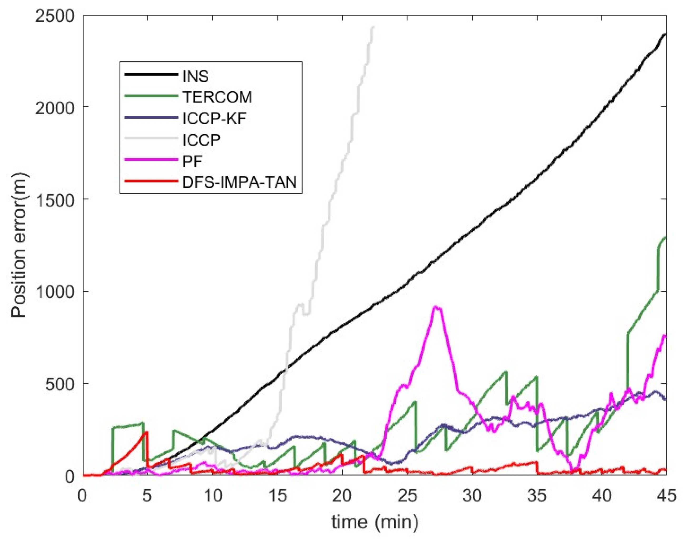
(3) Due to its periodic correction rather than real-time correction mechanism, the DFS-IMPA-TAN method exhibits slightly lower navigation accuracy than PF under favorable conditions, though it surpasses other batch-processing TAN methods. However, in terms of robustness, DFS-IMPA-TAN operates effectively under more challenging terrains and larger measurement errors, and possesses divergence self-correction capability. Thus, it demonstrates stronger robustness compared to other algorithms.

In summary, DFS-IMPA-TAN is a robust TAN framework. This framework enables AUVs to operate effectively in more complex environments, thereby expanding the range of TAN applications. DFS-IMPA-TAN can provide AUVs with robust underwater navigation, enabling them to adapt to various complex and dynamic underwater environments.

Future research will focus on integrating its stable navigation output with high-precision methods such as PF to achieve navigation solutions with higher accuracy and enhanced robustness.

References

1. Sahoo, A.; Dwivedy, S.K.; Robi, P.S. Advancements in the field of autonomous underwater vehicle. Ocean Eng. 2019, 181, 145–160. [Google Scholar] [CrossRef]
2. Bogur, R. Underwater robots: A review of technologies and applications. Ind. Robot An Int. J. 2015, 42, 186–191. [Google Scholar]
3. Zhang, H.W.; Zhang, J.C.; Liu, Y.H.; Wang, Y.H.; Wang, S.X.; Wu, Z.; Wang, F.; Hao, L.; Zheng, Y. Research on the influence of balance weight parameters on the motion performance of the seafloor mapping AUV in vertical plane. Ocean Eng. 2015, 109, 217–225. [Google Scholar] [CrossRef]
4. Fan, S.; Bose, N.; Liang, Z. Polar AUV Challenges and Applications: A Review. Drones 2024, 8, 413. [Google Scholar] [CrossRef]
5. Cheng, C.; Sha, Q.; He, B.; Li, G. Path planning and obstacle avoidance for AUV: A review. Ocean Eng. 2021, 235, 109355. [Google Scholar] [CrossRef]
6. Lapiere, L.; Zapata, R.; Lepinay, P.; Ropars, B. Karst exploration: Unconstrained attitude dynamic control for an AUV. Ocean Eng. 2020, 219, 108321. [Google Scholar] [CrossRef]
7. Lv, P.F.; Lv, J.Y.; Hong, Z.C.; Xu, L.X. Integration of Deep Sequence Learning-Based Virtual GPS Model and EKF for AUV Navigation. Drones 2024, 8, 441. [Google Scholar] [CrossRef]
8. Wang, R.P.; Wang, J.Y.; Li, Y.; Zhang, X. Research advances and prospects of underwater terrain-aided navigation. Remote Sens. 2024, 16, 2560. [Google Scholar] [CrossRef]
9. Ma, T.; Ding, S.S.; Li, Y.; Fan, J.J. A review of terrain-aided navigation for underwater vehicles. Ocean Eng. 2023, 281, 114779. [Google Scholar] [CrossRef]
10. Fan, G.; Han, Y.; Chen, P.Y.; Liu, Y.; Zhang, W.J.; Chung, C.Y.; Zhang, Y. A Self-Distillation Contrastive Learning Architecture for Global and Local Underwater Terrain Feature Extraction and Matching. IEEE Sens. J. 2024, 24, 20200–20218. [Google Scholar] [CrossRef]
11. Fan, G.; Liu, X.J.; Li, Y.; Li, J.; Han, Y.; He, L.; Chen, P.Y. A Terrain-Aided Navigation Method Incorporating Terrain Matching and Terrain Suitability Analysis. IEEE Access 2025, 13, 71066–71080. [Google Scholar] [CrossRef]
12. Zhao, S.W.; Deng, Z.H.; Zhang, W.Z.; Wang, Y. Adaptive Point Mass Filter and Its Application in Terrain Matching Navigation. IEEE Trans. Instrum. Meas. 2025, 74, 1–13. [Google Scholar] [CrossRef]
13. Zhou, T.; Peng, D.D.; Xu, C.; Zhang, W.Y.; Shen, J.J. Adaptive particle filter based on Kullback–Leibler distance for underwater terrain-aided navigation with multi-beam sonar. IET Radar Sonar Navig. 2018, 12, 433–441. [Google Scholar] [CrossRef]
14. Zhou, T.; Wang, T.H.; Gao, J.Q.; Guo, Q.J.; Yan, Z.Y. Particle filter underwater terrain-aided navigation based on gradient fitting. Meas. Sci. Technol. 2022, 33, 105009. [Google Scholar] [CrossRef]
15. Chai, X.J.; Li, Y.L.; Qiao, L. Terrain-aided navigation of long-range AUV based on cubature particle filter. IEEE Trans. Instrum. Meas. 2024, 73, 1–9. [Google Scholar] [CrossRef]
16. Yousuf, S.; Kadri, M.B. Improving the Position Accuracy and Computational Efficiency of UAV Terrain Aided Navigation Using a Two-Stage Hybrid Fuzzy Particle Filtering Method. CMC-Comput. Mater. Contin. 2025, 82, 1193–1210. [Google Scholar] [CrossRef]
17. Liu, Y.J.; Zhang, G.C.; Huang, Z.J. Study on the Arctic underwater terrain-aided navigation based on fuzzy-particle filter. Int. J. Fuzzy Syst. 2021, 23, 1017–1026. [Google Scholar] [CrossRef]
18. Ma, D.; Ma, T.; Li, Y.; Ling, Y.; Ben, Y.Y. A robust fusion terrain-aided navigation method with a single beam echo sounder. Ocean Eng. 2023, 286, 115610. [Google Scholar] [CrossRef]
19. Nordlund, P.J.; Gustafsson, F. Marginalized particle filter for accurate and reliable terrain-aided navigation. IEEE Trans. Aerosp. Electron. Syst. 2009, 45, 1385–1399. [Google Scholar] [CrossRef]
20. Kim, T.; Kim, J.; Byun, S.W. A comparison of nonlinear filter algorithms for terrain-referenced underwater navigation. Int. J. Control Autom. Syst. 2018, 16, 2977–2989. [Google Scholar] [CrossRef]
21. Lee, J.; Bang, H. A robust terrain-aided navigation using the Rao-Blackwellized particle filter trained by long short-term memory networks. Sensors 2018, 18, 2886. [Google Scholar] [CrossRef]
22. Salavasidis, G.; Munafò, A.; Fenucci, D.; Harris, C.A.; Prampart, T.; Templeton, R.; Smart, M.; Roper, D.T.; Pebody, M.; Abrahamsen, E.P.; et al. Terrain-aided navigation for long-range AUVs in dynamic under-mapped environments. J. Field Robot. 2020, 38, 402–428. [Google Scholar] [CrossRef]
23. Choe, Y.; Song, J.W.; Park, C.G. Lightweight marginalized particle filtering with enhanced consistency for terrain-referenced navigation. IEEE Trans. Aerosp. Electron. Syst. 2022, 58, 2493–2504. [Google Scholar] [CrossRef]
24. Zhang, J.Y.; Zhang, T.; Liu, S.D. An outlier-robust Rao–Blackwellized particle filter for underwater terrain-aided navigation. Ocean Eng. 2023, 288, 116006. [Google Scholar] [CrossRef]
25. Long, Z.; Gao, N.; Huang, B.Q. A novel terrain-aided navigation algorithm combined with the TERCOM algorithm and particle filter. IEEE Sens. J. 2015, 15, 1124–1131. [Google Scholar] [CrossRef]
26. Wang, R.P.; Li, Y.; Ma, T.; Cong, Z.; Gong, Y.; Xu, P.F. Improvements to terrain-aided navigation accuracy in deep-sea space by high precision particle filter initialization. IEEE Access 2020, 8, 13029–13042. [Google Scholar]
27. Wang, R.P.; Chen, Y.S.; Li, Y.; Xu, P.F.; Shen, P. High-precision initialization and acceleration of particle filter convergence to improve the accuracy and stability of terrain-aided navigation. ISA Trans. 2021, 110, 172–197. [Google Scholar]
28. Golden, J.P. Terrain contour matching (TERCOM): A cruise missile guidance aid. In Image Processing for Missile Guidance; SPIE: San Diego, CA, USA, 1980. [Google Scholar]
29. Li, P.J.; Sheng, G.L.; Zhang, X.F.; Wu, J.Q.; Xu, B.C.; Liu, X.; Zhang, Y. Underwater terrain-aided navigation system based on combination matching algorithm. ISA Trans. 2018, 78, 80–87. [Google Scholar] [CrossRef]
30. Wang, H.B.; Xu, X.S.; Zhang, T. Multipath parallel ICCP underwater terrain matching algorithm based on multibeam bathymetric data. IEEE Access 2018, 6, 48708–48715. [Google Scholar] [CrossRef]
31. Ding, P.; Cheng, X.H. A new contour-based combined matching algorithm for underwater terrain-aided strapdown inertial navigation system. Measurement 2022, 202, 111870. [Google Scholar] [CrossRef]
32. Zhang, J.Y.; Zhang, T.; Zhang, C.; Yao, Y.Q. An improved ICCP-based underwater terrain matching algorithm for large initial position error. IEEE Sens. J. 2022, 22, 16381–16391. [Google Scholar] [CrossRef]
33. Wang, D.; Liu, L.; Ben, Y.; Dai, P.; Wang, J. Seabed terrain-aided navigation algorithm based on combining artificial bee colony and particle swarm optimization. Appl. Sci. 2023, 13, 1166. [Google Scholar] [CrossRef]
34. Faramarzi, A.; Heidarinejad, M.; Mirjalili, S.; Gandomi, A.H. Marine predators algorithm: A nature-inspired metaheuristic. Expert Syst. Appl. 2020, 152, 113377. [Google Scholar] [CrossRef]
35. Yousri, D.A.; Fathy, A.A.; Rezk, H. A new comprehensive learning marine predator algorithm for extracting the optimal parameters of supercapacitor model. J. Energy Storage 2021, 42, 103035. [Google Scholar] [CrossRef]
36. Yang, Y.; Chen, H.; Heidari, A.A.; Gandomi, A.H. Hunger games search: Visions, conception, implementation, deep analysis, perspectives, and towards performance shifts. Expert Syst. Appl. 2021, 177, 114864. [Google Scholar] [CrossRef]
37. Abrahamsen, E.P. Gridded Bathymetric Compilation of Selected Areas Within the Orkney Passage, Scotia Sea From Multibeam Echosounder Data Collected by Multiple Vessels (1989–2017); UK Polar Data Centre; Natural Environment Research Council; UK Research & Innovation: Swindon, UK, 2020. [Google Scholar] [CrossRef]
38. Gao, W.; Zhao, B.; Zhou, G.T.; Wang, Q.Y.; Yu, C.Y. Improved Artificial Bee Colony Algorithm Based Gravity Matching Navigation Method. Sensors 2014, 14, 12968–12989. [Google Scholar] [CrossRef]
39. ZhongKeTuXin. 5 m Resolution DEM & DSM. 2025. Available online: http://www.tuxingis.com/resource/dem_5_download.html (accessed on 16 January 2025).
Figure 1. Impact of self-similar terrains on the PF.
Drones 09 00543 g001
Figure 2. Schematic illustration of self-similar terrain and local optimum terrain.
Drones 09 00543 g002
Figure 3. Flowchart of the IMPA-TAN.
Drones 09 00543 g003
Figure 4. Robust tree principles diagram.
Drones 09 00543 g004
Figure 5. Schematic of robust tree construction.
Drones 09 00543 g005
Figure 6. Flowchart of the DFS-IMPA-TAN algorithm.
Drones 09 00543 g006
Figure 7. DEM of the real seabed.
Drones 09 00543 g007
Figure 8. Results of the different algorithms for simulation test I.
Drones 09 00543 g008
Figure 9. Navigation errors of the different algorithms for simulation test I.
Drones 09 00543 g009
Figure 10. Results of the different algorithms for simulation test II.
Drones 09 00543 g010
Figure 11. Results of DFS-IMPA-TAN for simulation test II.
Drones 09 00543 g011
Figure 12. Navigation errors of DFS-IMPA-TAN for simulation test II.
Drones 09 00543 g012
Figure 13. Time consumption for processing of different trajectory segments in simulation test II.
Drones 09 00543 g013
Figure 14. The fitness values obtained by different algorithms in different rounds.
Drones 09 00543 g014
Figure 15. Equipment for the in-vehicle experiments.
Drones 09 00543 g015
Figure 16. DEM of Heimifeng Mountain.
Drones 09 00543 g016
Figure 17. Height measurement error of the in-vehicle experiment.
Drones 09 00543 g017
Figure 18. Results of the different algorithms for the first half of in-vehicle experiment.
Drones 09 00543 g018
Figure 19. Navigation errors of the different algorithms for the first half of in-vehicle experiment.
Drones 09 00543 g019
Figure 20. Mean errors of the different algorithms for the first half of in-vehicle experiment.
Drones 09 00543 g020
Figure 21. Navigation results of DFS-IMPA-TAN for the in-vehicle experiment and the correction effect of the robust tree.
Drones 09 00543 g021
Figure 22. Navigation errors of the in-vehicle experiment.
Drones 09 00543 g022