Drones and Deep Learning for Detecting Fish Carcasses During Fish Kills

Abstract

Fish kills are sudden mass mortalities that occur in freshwater and marine systems worldwide. Fish kill surveys are essential for assessing the ecological and economic impacts of fish kill events, but are often labor-intensive, time-consuming, and spatially limited. This study aims to address these challenges by exploring the application of unoccupied aerial systems (or drones) and deep learning techniques for coastal fish carcass detection. Seven flights were conducted using a DJI Phantom 4 RGB quadcopter to monitor three sites with different substrates (i.e., sand, rock, shored Sargassum). Orthomosaics generated from drone imagery were useful for detecting carcasses washed ashore, but not floating or submerged carcasses. Single shot multibox detection (SSD) with a ResNet50-based model demonstrated high detection accuracy, with a mean average precision (mAP) of 0.77 and a mean average recall (mAR) of 0.81. The model had slightly higher average precision (AP) when detecting large objects (>42.24 cm long, AP = 0.90) compared to small objects (≤14.08 cm long, AP = 0.77) because smaller objects are harder to recognize and require more contextual reasoning. The results suggest a strong potential future application of these tools for rapid fish kill response and automatic enumeration and characterization of fish carcasses.

1. Introduction

Fish kills are common in freshwater and marine systems worldwide and can involve anywhere from tens to millions of aquatic organism fatalities [1,2,3]. Fish kill environmental effects can be numerous and often coincide, such as cascading food web effects. Decomposition-related dissolved oxygen depletion and nutrient release are also common, the latter of which can promote the growth of toxin-producing phytoplankton [1,4,5]. Local economies are also often affected by decomposing carcasses that foul coastlines, attract pests, and harbor pathogens [3,6]. Methods that enable stakeholders to rapidly detect and enumerate carcasses are critical to identify and address the root cause of a fish kill event and mitigate as much environmental and ecological damage as possible.

Fish kill carcass detection and enumeration is often carried out via in situ visual surveys by walking along the shoreline or from research vessels [2,7,8,9]. To document shored carcasses, the surveyor identifies shored carcasses along transect lines (n ≥ 3) spanning ~100 m from the water’s edge, perpendicular to the coastline. To document floating or submerged carcasses, visible carcasses are identified within a specified area and/or time frame, and results are extrapolated to the rest of the study area. However, several parameters can affect the vertical and horizontal distribution of carcasses, including tides, currents, aquatic vegetation, waterbody morphology (e.g., bathymetry, surface area), weather (e.g., wind), carcass buoyancy, and scavenging animals [7]. It is estimated that floating fish kill surveys fail to enumerate about 80% of the carcasses due to turbidity and fish sinking to the bottom or being washed away [3,10]. Moreover, these methods can be labor and time-intensive, depending on sample site accessibility, carcass abundance and diversity, and surveyor expertise [9].

Unoccupied aerial systems (UAS), or drones, are a promising alternative to in situ surveys, as they allow users to collect high-resolution imagery of large areas within relatively short time frames [11]. Drones can also monitor sites with limited coastal access and can be flown at any time rather than having to adhere to satellite schedules. Drone imagery is also collected at high spatial resolutions, which can reduce the need for field validation data collection, as target objects can be observed at sufficient detail for identification. Drone imagery and deep learning methods have been tested to detect aquatic organisms such as sea cucumbers [12] and enumerate holes dug by burrowing animals [13]. Nocturnal thermal imagery has also been used to detect terrestrial mammals such as hare (Lepus europaeus) and roe deer (Capreolus capreolus) [14]. The deep learning model YOLO has been modified for real-time floating dead fish detection in inland aquaculture ponds using UAS imagery [15]. While these methods have proven useful, several limitations must also be considered during aerial monitoring.

As with in situ surveys [3,10], sinking carcasses and water turbidity can limit carcass detection from aerial imagery. Turbidity can limit aerial aquatic wildlife monitoring to floating individuals [15], partially submerged organisms such as the hippopotamus (Hippopotamus amphibius) [16] and surfacing organisms such as the finless porpoise (Porpoise neophocaena) [17]. Flight location, altitude, and time can also be restricted by aviation authorities, such as the Federal Aviation Administration (FAA) in the United States [18] and the Civil Aviation Safety Authority in Australia [19] to ensure public safety. Strong wind, precipitation, freezing temperatures, and sun glint can also restrict flight ability, visibility, and data processing [11,20].

This study aims to provide a novel tool for monitoring fish kills by (a) determining whether drone imagery provides sufficient resolution to identify floating and shored carcasses and (b) testing the feasibility of automating fish carcass detection from drone imagery by developing a deep learning model based on a single shot multibox detection (SSD) convolutional neural network (CNN). The SSD model was tested because it combines localization and classification in a single forward pass, which increases speed and efficiency. SSD not only predicts bounding box coordinates but also assigns class scores to each default box, indicating the likelihood of an object belonging to a specific category. SSD is often used for real-time object detection and has been used for automated bird detection from drone imagery [21]. Ultimately, the results from this study aim to provide a novel tool that can collect large amounts of data with minimal effort, leading to a much-needed, better understanding and management of fish kill events [1].

2. Materials and Methods

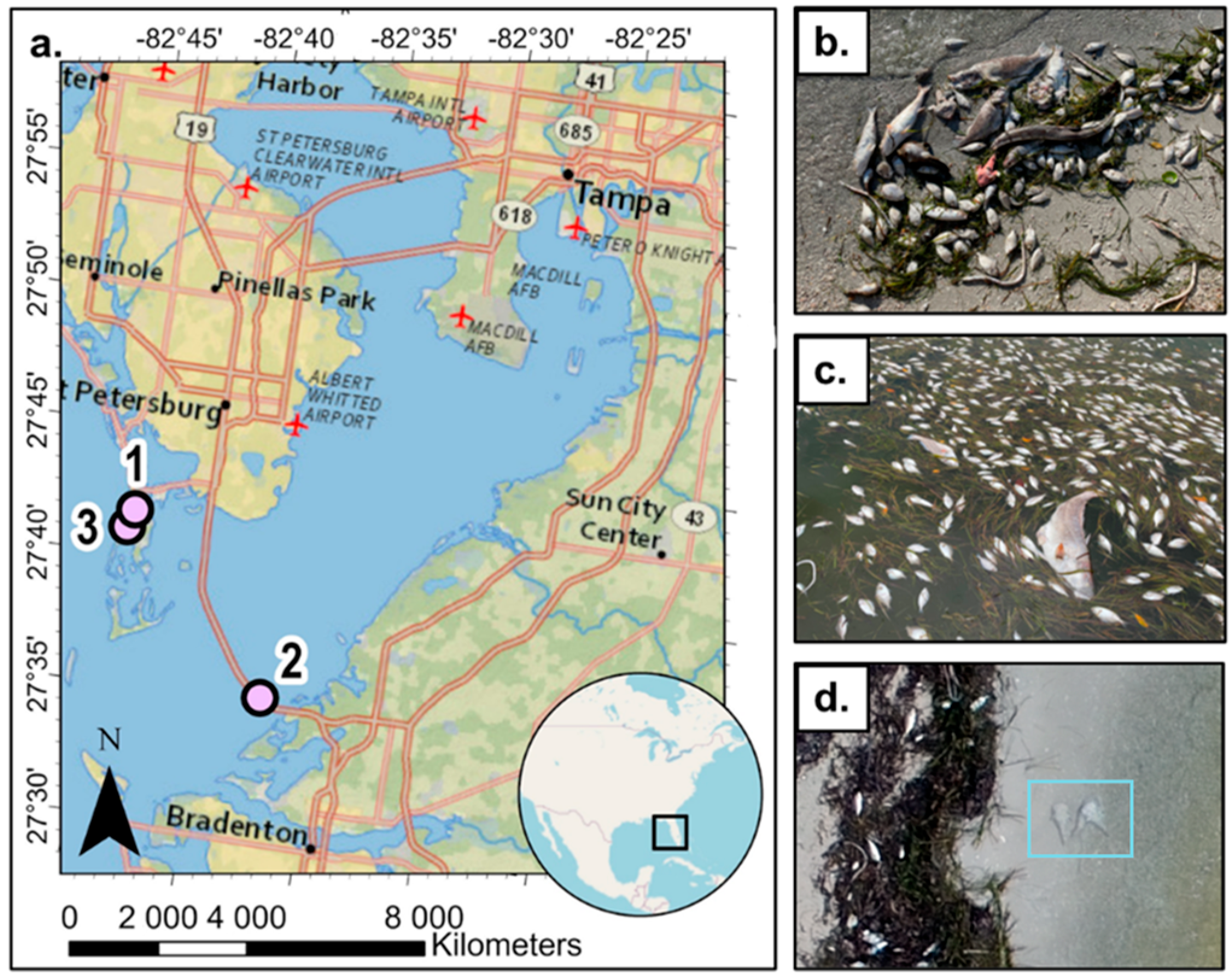
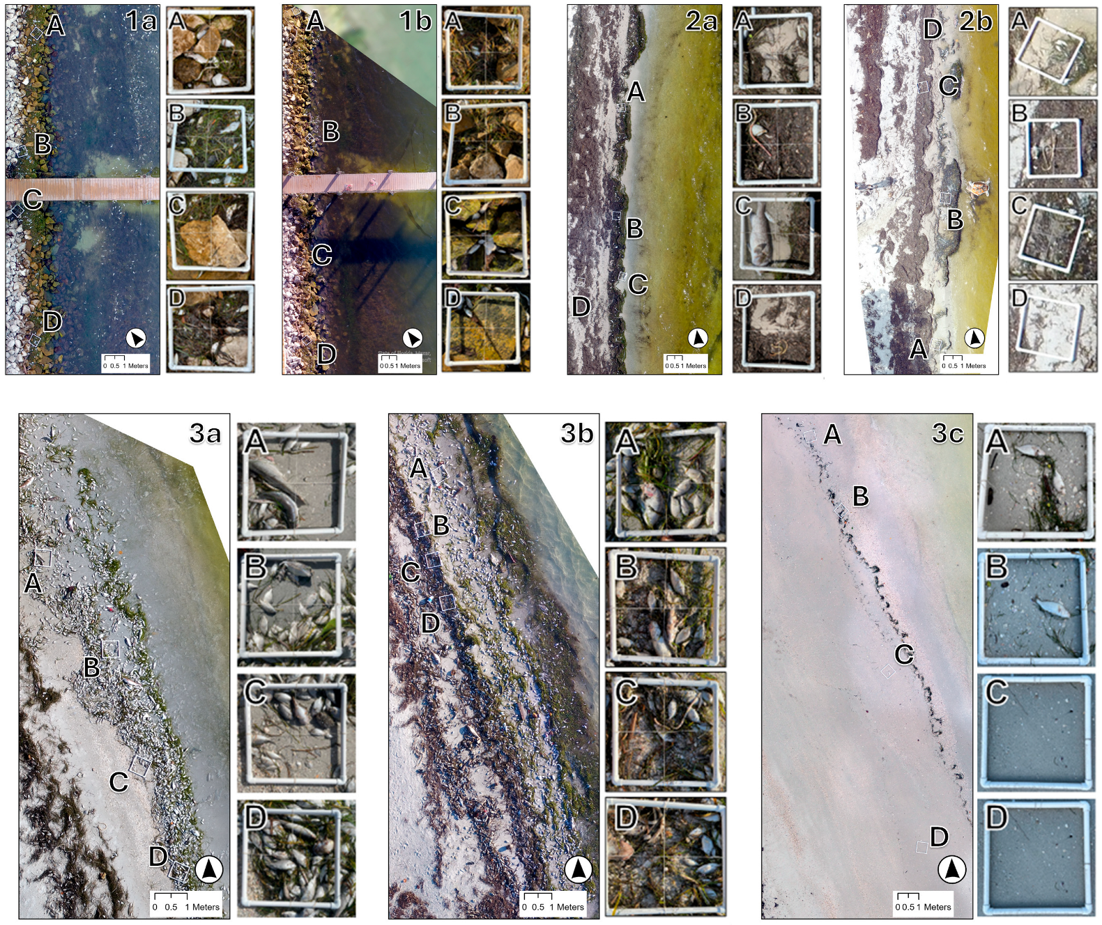
2.1. Study Sites

The seven drone flights were conducted from 13 July 2021 to 10 December 2022 during two coastal fish kill events in Tampa Bay, FL (

Table 1. All drone flights were conducted using a DJI Phantom 4 quadcopter, with an onboard RGB sensor pointed at nadir (90° horizontal). Flight planning was completed using the Pix4Dcapture mobile device application. The number of marked, or annotated, tiles per flight is included (marked tile count/total tile count).

Flight ID	Site ID	Date	Start Time	Flight Time (min.sec)	Flight Dim (m)	Flight Alt (m)	GSD (cm/pixel)	Temp (°C)	Solar Altitude	Azimuth	Marked Tiles
1a	1	13 July 2021	7:42 PM	5.50	17 × 46	9.8	0.44	27	11.51	71.29	20/480
1b	1	14 July 2021	8:01 AM	5.23	17 × 46	9.8	0.44	26	14.99	73.13	17/437
2a	2	14 July 2021	11:02 AM	6.27	17 × 53	9.8	0.44	29	54.42	91.2	36/341
2b	2	15 July 2021	4:18 PM	6.32	17 × 53	9.8	0.44	32	53.03	269.22	34/286
3a	3	14 July 2021	9:19 AM	5.16	17 × 46	9.8	0.44	27	31.75	80.58	45/560
3b	3	16 July 2021	7:51 AM	5.22	17 × 46	9.8	0.44	28	12.71	72.41	35/234
3c	3	10 December 2022	8:02 AM	14.54	28 × 162	10.3	0.40	18	10.74	123.17	11/2328

Alt = altitude, Dim = dimensions, GSD = ground sampling distance, min.sec = minutes.seconds, Temp = temperature.

). Six flights (flights 1a–3b) were conducted during a 2021 summer fish kill, which coincided with a red tide event as well as the passage of Tropical Storm Elsa (Tampa Bay landfall 07/05/21) [22]. By August 2021, more than 1600 metric tons of dead fish had reportedly been cleaned up from public and private shorelines. One flight (flight 3c) was conducted during a fish kill in winter 2022, which coincided with a red tide event that preceded Hurricane Ian (Category 4, US landfall 09/23/22) [23].

Three sites were selected based on carcass abundance, FAA drone airspace restrictions [18], accessibility and safety of take-off and landing areas, differences in beach substrate (i.e., sandy and rocky), and presence of Sargassum washed ashore (Figure 1). Site 1 (27.695665 N, −82.732309 W) was a rocky intertidal seawall with abundant Sargassum and fish carcasses. Site 2 (27.653359 N, −82.675608 W) was a sandy beach underpass at the mouth of Tampa Bay with high Sargassum and fish carcasses at various stages of decomposition. Site 3 (27.653359 N, −82.675608 W) was a sandy intertidal site along a seawall with various carcass abundances.

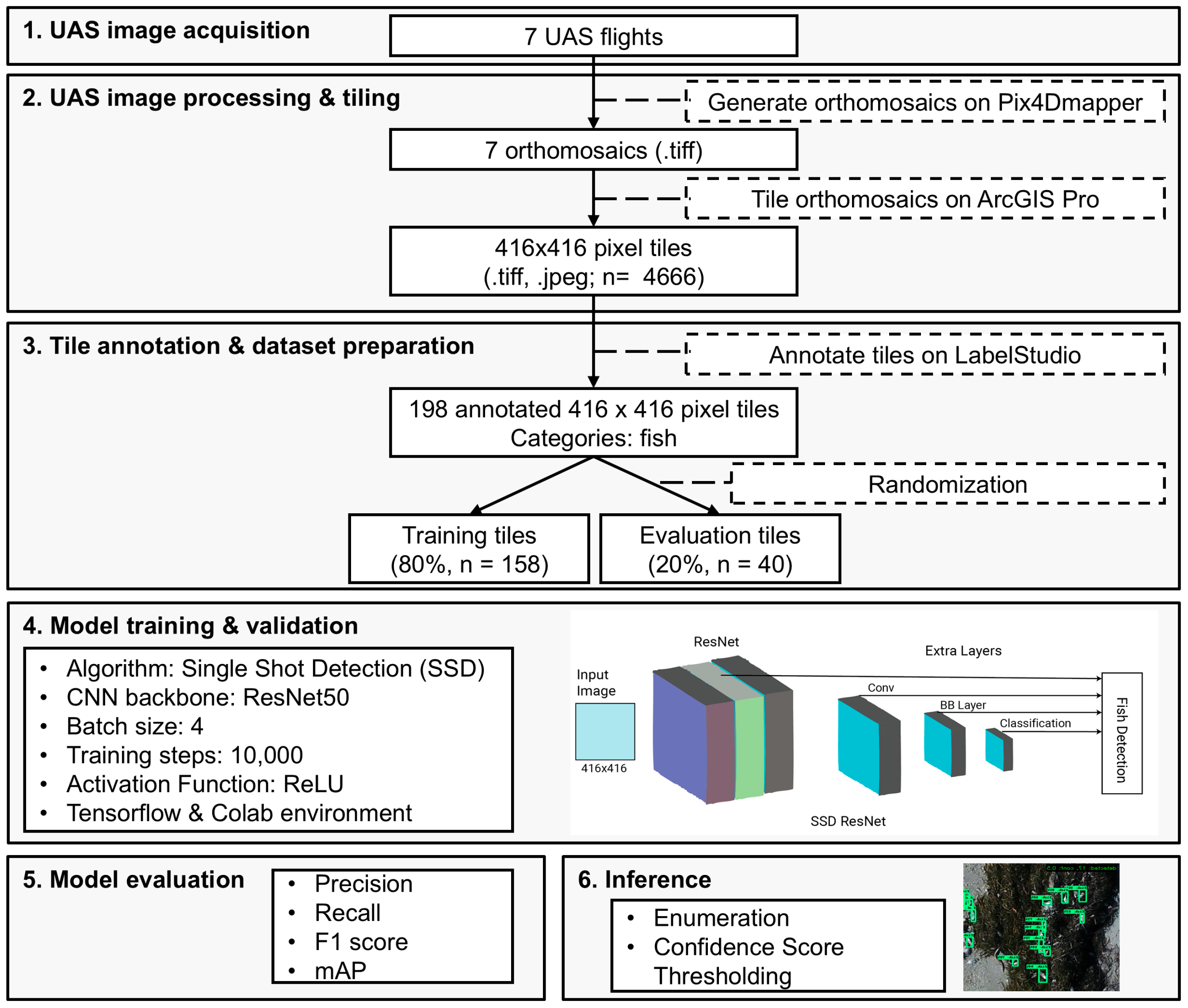
2.2. Drone Image Acquisition

Aerial images were collected using a DJI Phantom 4 (DJI, Shenzhen, China) quadcopter’s integrated 12.4 M RGB (red, green, blue) sensor (specifications: 94°20 mm field of view, 20 mm focal length). The DJI Phantom 4 was equipped with a GPS/GLONASS integrated system that GPS-tagged the images with latitude, longitude, and altitude information.

The free mobile device application Pix4Dcapture was used to automate UAS flights. All flights were conducted with the sensor pointed at nadir (90° horizontal), with a 75% side and 75% front overlap, a fast picture trigger mode, and automatic white balance (Table 1). Flights were conducted on clear days with wind speeds ≤15 km/h.

2.3. Drone Image Processing and Tiling

Pix4Dmapper version 4.8.4 (Lausanne, Switzerland) software was utilized to generate point cloud densification, digital surface models (DSM), orthomosaics, and reflection maps for the seven flights (Figure 2 and Figure 3). Orthomosaics were generated by calculating the weighted average of the pixels in the original images. The seven orthomosaics were tiled to a standardized resolution of 416 × 416 pixels to reduce computational complexity and satisfy the data input requirements for the single shot multibox detection-ResNet50 model required by the convolutional neural network. The split raster tool in ArcGIS Pro 3.1.1 was used to split orthomosaics into 416 × 416 pixel tiles with a 10-pixel overlap. Tiles were generated as both TIFF and PNG files.

2.4. Drone Image Annotation

The 416 × 416 pixel tiles were uploaded to the data labeling platform Label Studio [24] for manual carcass identification and annotation. All visible carcasses were annotated using the template for object detection with bounding boxes annotation. Annotations were limited to carcasses washed ashore because water movement changed the position of the fish in the water, preventing tie point generation (Figure 1d). A single object category, “fish”, was included in the labeling process. The number of annotated, or marked, tiles for each orthomosaic is specified in Table 1. The 198 annotated tiles from the seven aerial flights were used for deep learning model training purposes, and the labels were formatted in the Pascal VOC XML format.

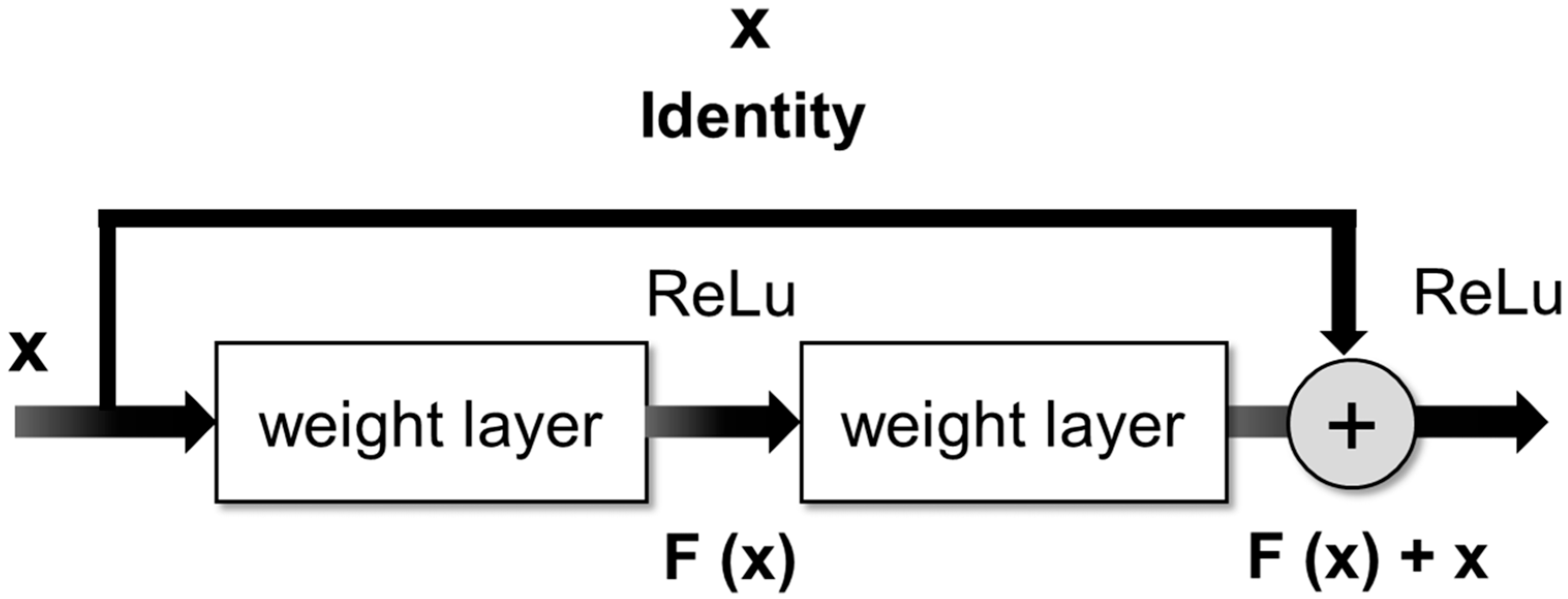
2.5. Model Architecture and Training

An open-source deep learning object detection algorithm, single shot multibox detection, with ResNet50 as the backbone was utilized to detect and enumerate carcasses. Single shot multibox detection utilizes a single forward pass to locate and classify objects using bounding box regression [25]. Single shot multibox detection begins the detection process based on precomputed fixed-size bounding boxes called priors, which closely match the distribution of bounding boxes in the annotated training images. By applying a 3 × 3 filter, single shot multibox detection predicts the four coordinates (x, y, w, h) to determine the difference between observed and predicted bounding boxes. ResNet50, a convolutional neural network with 50 layers, was used as the backbone network [26].

The ResNet architecture consists of stacked residual blocks [26]. These blocks have a special shortcut connection that skips one or more layers during training (Figure 4). The skip connection bypasses some levels in between link-layer activations to subsequent layers. This creates a leftover block. These leftover blocks are stacked to create ResNets. The strategy behind this network is to let the network fit the residual mapping rather than have layers learn the underlying mapping [27].

The single shot multibox detection-ResNet50 model was trained using the 416 × 416 annotated tiles generated (n = 198). The training data was split into an 80–20% train–test split, with 80% used for training (n = 158) and 20% for evaluation (n = 40). Model development was conducted in the Google Colab environment with TensorFlow Version 2.10.0 [28]. Different iterations of the model were conducted to find the best hyperparameters including initial learning rate, number of iterations (i.e., steps and batch size). The optimizer for the network was set as stochastic gradient descent and the initial learning rate was 0.039 with a momentum of 0.89. To improve our model’s performance, we used a warm-up training approach during the initial phase of training. At the beginning of training, we gradually increased the learning rate from 0.0133 over the first 2000 steps (approximately two epochs) to the base learning rate of 0.039. After the warm-up phase, the learning rate remained at 0.04 and followed a cosine decay schedule for the remainder of the training. The total training took a total of 10,000 steps to achieve a stable convergence result. A total of 50 weight checkpoints were generated at each 200 steps for post-training validation of the model.

ReLU activation was used for feature extraction and box predictor (Figure 4). The activation parameter was set to ReLU 6, which clips all negative values to zero and all positive values above 6 to 6. In comparison with ReLU, ReLU 6 activation functions have been shown to empirically perform better under low-precision conditions (e.g., fixed point inference) by encouraging the model to learn sparse features earlier [29].

2.6. Loss Metrics

During training, different loss functions were implemented to evaluate how the algorithm was modeling the data. The loss consisted of three components: localization, classification, and regularization loss. Object localization is the task of determining the position of an object or multiple objects in an image/frame with the help of a rectangular box around an object, commonly known as a bounding box [30]. The localization loss was used as a measure of bounding box offset prediction. Smooth L₁ loss function was used to quantify the localization loss. Smooth L₁ between predicted value $\widehat{y}$ and target value y is given as:

$$L_{1;smooth}=\left\{\begin{array}{c}0.5{(\widehat{y}-y)}^2, if\left|\widehat{y}-y\right|<1\\ \widehat{|y}-y|-0.5, otherwise\end{array}\right.$$

(1)

The classification loss was used for conditional class probabilities. Sigmoid focal loss function was used to quantify the classification loss. The sigmoid focal loss function is given as:

$$L\left(y,p\right)=-\alpha {\left(1-p\right)}^{\gamma }log\left(p\right)-\left(1-\alpha \right)p^{\gamma }log(1-p)$$

(2)

where

y = ground truth label (0, 1)

p = class probability

$\alpha$ = balancing parameter, which was initially set to 0.25

$\gamma$ = the focusing parameter, which was initially set to 2.

To make the model simpler so that it generalized better, L2 regularization was introduced. L2 regularization adds a penalty for large weights in a model, reducing overfitting. L2 regularization is expressed in terms of weights as:

$$L2Regularization=\lambda {\sum }_i{w}_i^2$$

(3)

Total loss was calculated as the sum of the abovementioned three loss metrices. Only total loss metrics were calculated for the validation dataset as accuracy metrices were calculated, whereas all three loss metrices were calculated for the training dataset.

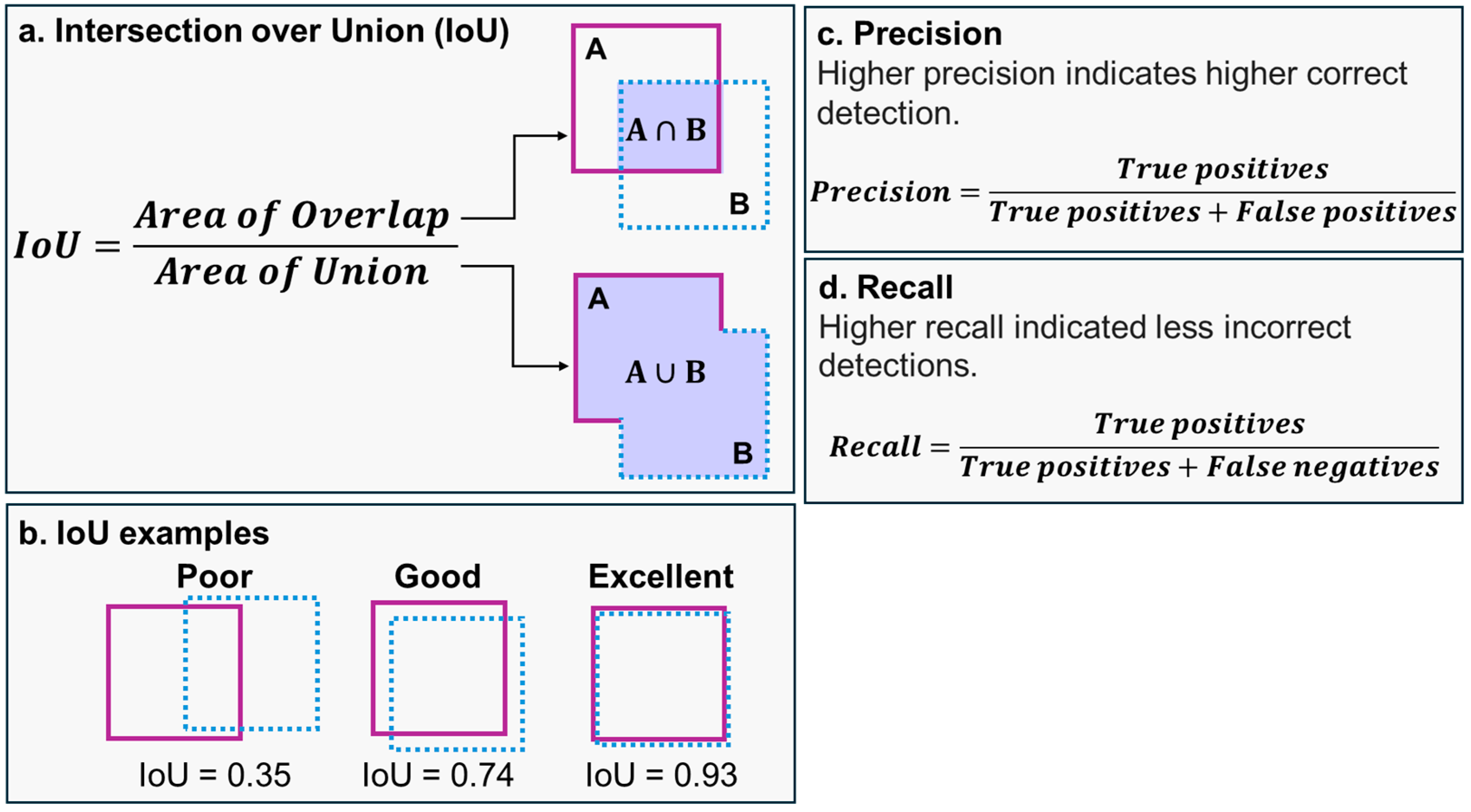
2.7. Evaluation Metrics

The performance of the object detection was evaluated using the common objects in context (COCO) application programming interface (API), which is based on COCO datasets [31,32]. The COCO API provides a way to evaluate an object detection model based on AP (average precision) and IoU (intersection over union). AP was calculated with different IoU thresholds (0.5 and 0.75) and areas (all, small, medium, large) to assess the accuracy of object detection. The COCO metrics benchmark defines small objects as those with an area between 0 and 32 × 32 (1024) square pixels, medium objects between 1024 and (96 × 96) 9216 square pixels, and large objects above 9216 square pixels. Generally, smaller objects are harder to recognize and require more contextual reasoning to recognize [31].

IoU is used to measure localization accuracy and compute localization errors in object detection models by calculating the overlap between the predicted bounding box (A) and the area of the manually labeled bounding box (B; Figure 5a,b) [33].

$$IoU={\displaystyle \frac{TP}{TP+FP+FN}}$$

(4)

where true positive (TP) represents the correctly detected fish carcasses, false positive (FP) represents incorrectly detected fish carcasses, false negative (FN) represents missed detections, and true negative (TN) represents correct identification of absence when there should be none.

Two IoU thresholds were tested to characterize true positive detections. This was accomplished by stipulating that a minimum of 50% (IoU = 0.50) or 75% (IoU = 0.75) of the bounding box area identified by the detected bounding box (A) should overlap with the corresponding manually labeled bounding box (B). A higher IoU threshold signifies greater precision but can lead to a decrease in true positive detections.

A confusion matrix is a table used to summarize the performance of a machine learning model by comparing the model’s predictions to the manually generated labels (i.e., ground-truthing; Figure 5c). The four entries for the confusion matrix included instances where the model correctly predicted the positive class (or true positives; TP); instances where the model correctly predicted the negative class (true negatives; TN), instances where the model incorrectly predicted the positive class (false positives; FP; type I error), and instances where the model incorrectly predicted the negative class (false negatives; FN; type II error). The TP, TN, FN, and FP counts are used to calculate evaluation metrics such as precision, recall, and mean average precision (MAP).

Precision is used to estimate the accuracy of a model’s true positive predictions by assessing the ratio of correctly identified positive predictions (true positives) to the sum of detected positive predictions (true positives + false positives), based on manually labeled data (Figure 5d). Meanwhile, recall estimates the model’s ability to correctly identify positive instances, calculated as the ratio of true positives to the sum of true positives and false negatives (Figure 5d). A trade-off often exists between precision and recall; an increase in detection tends to boost recall but might lead to reduced precision due to an increase in false positives. Precision values range from 0, indicating very low precision, to 1, representing perfect precision. Similarly, recall values range from 0, indicating poor recall, to 1, indicating perfect recall. Elevated recall implies fewer incorrect detections, or lower detection of objects that are not fish carcasses.

mAP is a performance metric that calculates the average precision across different levels of recall and then takes the mean over a set of queries or classes, providing an overall measure of retrieval accuracy. The mean average precision is represented as:

$$mAP={\displaystyle \frac{1}{n}}\sum _{k=1}^{k=n}{AP}_k$$

(5)

where

n = number of classes (n = 1)

AP_k = the average precision of classes k

2.8. Fish Species Composition Estimates and Length Measurements

Quadrat surveys were conducted to estimate carcass diversity and abundance, and to improve tie point detection during orthomosaic generation. While the quadrats provided useful baseline data to better understand carcass size and composition, the carcass detection model was applied to the entire study area rather than just the quadrats. A total of 24 quadrats were enumerated during seven surveys conducted at three sites from 7/13/21 to 12/10/22 (Table 1, Figure 3). Surveys were conducted by placing three to four 0.5 m² PVC quadrats randomly throughout the shoreline to the high tide mark. Fish were counted when >50% of their body was within the quadrat, identified to the category level, and measured from the tip of the snout to the end of the longer lobe of the caudal fin (

Table 2. Carcass mean length and counts from quadrat surveys. Total carcass count n = 181.

Fish Group	Mean Length (cm)	SD	Count
American eel	54.48	13.19	8
American shad/ Scaled sardine/ Atlantic thread herring	10.16	n.a.	1
Black grouper	71.94	n.a.	1
Grunt	19.32	0.45	2
Mullet	37.17	9.37	4
Pinfish	12.03	4.25	147
Scrawled cowfish	17.04	5.46	3
Sea robin	12.76	3.95	3
Spotted seatrout	49.83	n.a.	1
Striped burrfish	14.91	1.95	4
Toadfish	22.55	12.88	7

n.a. = not available.

). Fish identification resources included A Field Guide to Coastal Fishes: From Maine to Texas [34] and the Florida Fish and Wildlife Conservation Commission (FWC) Species Profiles webpage [35].

3. Results

The 181 carcasses measured 15.64 cm on average (S.D. = 11.9 cm) and ranged in length from small baitfish (10.16 cm) to a large black grouper (Mycteroperca bonaci, 71.94 cm; Table 2). Carcasses also varied in morphology, state of decomposition, and spatial distribution (Figure 1b,c and Figure 5).

Shored fish carcasses were clearly visible from drone imagery, suggesting that the ground sampling distance of 0.44 cm/pixels was adequate to visually detect the presence/absence of shored carcasses (Figure 3). However, the resolution was not high enough to confidently determine fish species from drone imagery. Moreover, it was not possible to detect floating carcasses due to water movement changing the carcass location between images and creating “ghost” fish (Figure 1d). Detection of submerged carcasses was also limited by turbidity and poor orthomosaic generation over large areas of water.

The proposed method for automatic detection of shored fish carcasses based on single shot multibox detection ResNet50 showed good performance in predicting the fish carcasses of sizes ranging from small (≤14.08 cm long) to large (>42.24 cm long). The mean average precision (mAP) of predicting the fish carcasses was 0.773 with a mean average recall (mAR) of 0.810 [AR@100, 0.50:0.95 IoU] (

Table 3. Performance metrics summary for fish carcass detection.

Metric	IoU Range	Object Area	Max Detections	AP	AR
Average Precision (AP)	0.50:0.95	All	100	0.773	0.810
Average Precision (AP)	0.50	All	100	0.979
Average Precision (AP)	0.75	All	100	0.951
Average Precision (AP)	0.50:0.95	Small	100	0.769	0.807
Average Precision (AP)	0.50:0.95	Medium	100	0.822	0.851
Average Precision (AP)	0.50:0.95	Large	100	0.900	0.900
Average Recall (AR)	0.50:0.95	All	1		0.049
Average Recall (AR)	0.50:0.95	All	10		0.361
Average Recall (AR)	0.50:0.95	All	100	0.773	0.810
Average Recall (AR)	0.50:0.95	Small	100	0.769	0.807
Average Recall (AR)	0.50:0.95	Medium	100	0.822	0.851
Average Recall (AR)	0.50:0.95	Large	100	0.900	0.900

IoU = intersection over union.

). The model had slightly higher average precision (AP) when detecting large objects (>42.24 cm long, AP = 0.900, IoU 0.50:0.95) compared to small objects (≤14.08 cm long, AP = 0.769, IoU 0.50:0.95), as smaller objects are harder to recognize and require more contextual reasoning to recognize. The average recall (AR) improved as the allowed number of detections increased from 1 (AR = 0.049) to 100 (AR = 0.810) and was consistently strong (AR > 0.807) across object sizes.

The loss of the training model denotes the sum of all losses of the model for each training and validation dataset (Figure 6). The blue curve represents the overall loss trend of the model while training, and the orange curve represents the loss during the validation phase. Both curves show a downward trend, suggesting less and less information was lost during the training process. To make sure the model was not overfitting, we produced model checkpoints every 200 steps which were used for post-training validation. The validation curve shows there was no issue with overfitting the model. The model started to converge around 6000 steps. Figure 7 includes four example inferenced images, where bounding boxes and detection confidences are plotted on each identified carcass.

4. Discussion

4.1. Monitoring Shored Carcasses

The study demonstrated that drone imagery and deep learning, specifically single shot multibox detection with a ResNet50 backbone, were reliable tools for remotely detecting fish carcasses washed ashore during fish kill events (Table 3). The image resolution (0.44 cm/pixel) proved useful for detecting carcasses, particularly larger carcasses (>42.24 cm). The model performed better on larger carcasses because they appear more clearly in aerial images and have more visible features. The shape, texture, and contrast make them easier for the model to detect.

The image resolution was insufficient for identifying carcass species, partially due to decomposition-caused carcass bloating and pigmentation loss. These rapid morphologic changes can complicate identification at in situ resolution and become more challenging through aerial surveys (Figure 1) [36]. To improve carcass identification, imagery could be collected at a higher resolution by flying the drone at a lower altitude or utilizing a drone equipped with a higher-resolution sensor. Shored carcass aerial surveys should also be conducted close to solar noon to minimize shadows and maximize lighting of the survey area. However, solar noon should be avoided when collecting floating carcass data, as glint could reduce visibility at higher solar angles [17,20].

Despite these limitations, it was possible to characterize carcasses based on body morphology (i.e., baitfish, eel, sea turtle, grouper). Object categorization methods have been developed to differentiate between agricultural crops and weeds from drone imagery [37] and could serve as a baseline to develop models for carcass categorization.

4.2. Monitoring Floating Carcasses

While the drone imagery was useful for detecting fish carcasses washed ashore, the study methods tested were not useful for detecting floating or submerged carcasses due to poor orthomosaic generation over water, high turbidity, and “ghost” fish generation (Figure 1d and Figure 3).

Orthomosaic generation was successful for all the flights conducted and proved useful for monitoring shored carcasses. However, the orthomosaics excluded images captured past the coastline (Figure 3(1b,2b,3b)). This is an artifact of orthomosaic generation. Aerial imagery was captured at a fixed altitude and regular spatial intervals (75% side and front overlap; Table 1). Sufficient image overlap is necessary to identify key points needed for aligning images during orthomosaic generation. Identifying key points is challenging over homogeneous and fluid water, leading to incomplete or failed orthomosaic generation over large areas of water [11]. To remedy this issue, floating ground control points (GCPs) can be arranged throughout the survey area that will serve as reference points away from shore. However, GCP integration will increase the survey time and require additional equipment such as research vessels (e.g., kayaks, power boats) and georeferencing tools.

The floating fish carcasses captured in the near-shore area of the orthomosaics could not be enumerated accurately due to carcasses frequently appearing in multiple images, creating duplicate “ghost” fish (Figure 1d). By default, overlapping images will capture the same object multiple times. This method is ideal for monitoring stationary objects on solid mediums (i.e., sand), but is ineffective over fluid mediums such as water because water movement shifts the object location between images. During the orthomosaic generation process, the software assumed the key points were stationary, leading to misaligned pixels that were then averaged during orthomosaic generation, creating the “ghost” fish (Figure 1d). This processing issue has been reported when monitoring non-stationary animals in terrestrial ecosystems [38]. While it was clear when one fish was being captured several times when there were few fish present, it was not possible to differentiate between individual carcasses as their number increased within the raw imagery and orthomosaic, and therefore, these data were excluded from the study results.

To overcome both the issues related to poor orthomosaic generation over water and “ghost” fish, future surveys could consider capturing video footage rather than imagery [39]. Video footage could facilitate additional research approaches, such as real-time detection, but presents unique challenges, including dealing with duplicate carcasses moved by wave action. Video surveys over water should also be conducted early in the morning or late in the afternoon when the solar altitude is less than 40° to avoid the sun glint effect [17,20].

5. Conclusions

Results from this study suggest that drones are a feasible tool for detecting carcasses washed ashore. Deep learning methods proved effective for automating the carcass detection process, particularly when detecting large carcasses. Drones provided a less labor-intensive alternative for detecting carcasses over large areas, and the rapid improvements in commercial drones will likely relieve some of the current limitations through improved performance under adverse weather conditions, longer flight times, and higher sensor resolution.

While the aerial photographs collected by the drone were not useful for monitoring floating carcasses, future research should explore the use of video recordings to address this limitation. Moreover, studies that build on this model for carcass categorization and enumeration, surveys over different benthic covers and organisms of various morphologies, and potentially real-time detection, are required [15]. Ultimately, these technologies show promise for optimizing cleanup efforts and reducing the ecological and economic impacts of fish kill events by allowing users to collect large amounts of data with minimal physical effort. These techniques could be further applied to additional observed categories, such as benthic organisms or beach litter.

References

1. La, V.T.; Cooke, S.J. Advancing the science and practice of fish kill investigations. Rev. Fish. Sci. 2011, 19, 21–33. [Google Scholar] [CrossRef]
2. Meyer, F.P.; Barclay, L.A. Field Manual for the Investigation of Fish Kills; U.S. Fish and Wildlife Service: Washington, DC, USA, 1990. [Google Scholar]
3. Thronson, A.; Quigg, A. Fifty-five years of fish kills in Coastal Texas. Estuaries Coasts 2008, 31, 802–813. [Google Scholar] [CrossRef]
4. Holmlund, C.M.; Hammer, M. Ecosystem services generated by fish populations. Ecol. Econ. 1999, 29, 253–268. [Google Scholar] [CrossRef]
5. Vanni, M.J.; Luecke, C.; Kitchell, J.F.; Allen, Y.; Temte, J.; Magnuson, J.J. Effects on lower trophic levels of massive fish mortality. Nature 1990, 344, 333–335. [Google Scholar] [CrossRef]
6. Tribune News Service. Algal blooms can wreak havoc on Florida economy. Tampa Bay Times, 21 January 2024. [Google Scholar]
7. American Fisheries Society. Investigation and Valuation of Fish Kills; American Fisheries Society, Southern Division, Pollution Committee: Bethesda, MD, USA, 1992; ISBN 978-0-913235-81-2. [Google Scholar]
8. Powers, S.P.; Blanchet, H. Investigate Plan for Fish and Invertebrate Kills in the Northern Gulf of Mexico. MC 252 NRDA Fish Technical Working Group; 2010. Available online: https://www.google.com.hk/url?sa=t&source=web&rct=j&opi=89978449&url=https://www.fws.gov/doiddata/dwh-ar-documents/824/DWH-AR0013020.pdf&ved=2ahUKEwjPr5qU4KyOAxUF-aACHZEbH7MQFnoECBUQAQ&usg=AOvVaw31_k2zc8q05PvjocqaWOmB (accessed on 1 July 2025).
9. Virginia Department of Environmental Quality. Fish Kill Investigation Guidance Manual; Water Quality Standards and Biological Monitoring Programs: Richmond, Virginia, 2002.
10. Biernacki, E. Fish Kills Caused by Pollution.; U.S. Environmental Protection Agency: Washington, DC, USA, 1979.
11. Fernandez-Figueroa, E.G.; Wilson, A.E.; Rogers, S.R. Commercially available unoccupied aerial systems for monitoring harmful algal blooms: A comparative study. Limnol. Oceanogr. Methods 2022, 20, 146–158. [Google Scholar] [CrossRef]
12. Li, J.Y.Q.; Duce, S.; Joyce, K.E.; Xiang, W. SeeCucumbers: Using Deep Learning and Drone Imagery to Detect Sea Cucumbers on Coral Reef Flats. Drones 2021, 5, 28. [Google Scholar] [CrossRef]
13. Grigusova, P.; Larsen, A.; Achilles, S.; Klug, A.; Fischer, R.; Kraus, D.; Übernickel, K.; Paulino, L.; Pliscoff, P.; Brandl, R.; et al. Area-Wide Prediction of Vertebrate and Invertebrate Hole Density and Depth across a Climate Gradient in Chile Based on UAV and Machine Learning. Drones 2021, 5, 86. [Google Scholar] [CrossRef]
14. Povlsen, P.; Bruhn, D.; Durdevic, P.; Arroyo, D.O.; Pertoldi, C. Using YOLO Object Detection to Identify Hare and Roe Deer in Thermal Aerial Video Footage—Possible Future Applications in Real-Time Automatic Drone Surveillance and Wildlife Monitoring. Drones 2024, 8, 2. [Google Scholar] [CrossRef]
15. Zhang, H.; Tian, Z.; Liu, L.; Liang, H.; Feng, J.; Zeng, L. Real-time detection of dead fish for unmanned aquaculture by yolov8-based UAV. Aquaculture 2025, 595, 741551. [Google Scholar] [CrossRef]
16. Inman, V.L.; Leggett, K.E.A. Hidden Hippos: Using Photogrammetry and Multiple Imputation to Determine the Age, Sex, and Body Condition of an Animal Often Partially Submerged. Drones 2022, 6, 409. [Google Scholar] [CrossRef]
17. Morimura, N.; Itahara, A.; Brooks, J.; Mori, Y.; Piao, Y.; Hashimoto, H.; Mizumoto, I. A Drone Study of Sociality in the Finless Porpoise (Neophocaena asiaeorientalis) in the Ariake Sound, Japan. Drones 2023, 7, 422. [Google Scholar] [CrossRef]
18. Federal Aviation Administration. Part 107—Small Unmanned Aircraft Systems; Federal Aviation Administration, Department of Transportation: Washington, DC, USA, 2023.
19. Civil Aviation Safety Authority. Part 101 (Unmanned Aircraft and Rockets) Manual of Standards; Australian Department of Infrastructure, Transport, Regional Development, Communications, Sport and the Arts: Canberra, Australia, 2019.
20. Nahirnick, N.K.; Reshitnyk, L.; Campbell, M.; Hessing-Lewis, M.; Costa, M.; Yakimishyn, J.; Lee, L. Mapping with confidence; delineating seagrass habitats using Unoccupied Aerial Systems (UAS). Remote Sens. Ecol. Conserv. 2019, 5, 121–135. [Google Scholar] [CrossRef]
21. Hong, S.-J.; Han, Y.; Kim, S.-Y.; Lee, A.-Y.; Kim, G. Application of Deep-Learning Methods to Bird Detection Using Unmanned Aerial Vehicle Imagery. Sensors 2019, 19, 1651. [Google Scholar] [CrossRef] [PubMed]
22. Beck, M.W.; Altieri, A.; Angelini, C.; Burke, M.C.; Chen, J.; Chin, D.W.; Gardiner, J.; Hu, C.; Hubbard, K.A.; Liu, Y.; et al. Initial estuarine response to inorganic nutrient inputs from a legacy mining facility adjacent to Tampa Bay, Florida. Mar. Pollut. Bull. 2022, 178, 113598. [Google Scholar] [CrossRef]
23. Sarasota Bay Estuary Program Director’s Note: Red Tide and Fish Kills—Likely Effects of Hurricane Ian, and Scalability of Management Paradigms. Available online: https://sarasotabay.org/directors-note-red-tide-and-fish-kills-likely-effects-of-hurricane-ian-and-scalability-of-management-paradigms/ (accessed on 6 March 2024).
24. Tkachenko, M.; Malyuk, M.; Holmanyuk, A.; Liubimov, N. Label Studio: Data Labeling Software 2022. Available online: https://github.com/heartexlabs/label-studio (accessed on 1 July 2025).
25. Liu, W.; Anguelov, D.; Erhan, D.; Szegedy, C.; Reed, S.; Fu, C.-Y.; Berg, A.C. SSD: Single Shot MultiBox Detector. In Proceedings of the Computer Vision—ECCV 2016, Amsterdam, The Netherlands, 11–14 October 2016; Leibe, B., Matas, J., Sebe, N., Welling, M., Eds.; Springer International Publishing: Cham, Switzerland, 2016; pp. 21–37. [Google Scholar]
26. He, K.; Zhang, X.; Ren, S.; Sun, J. Deep Residual Learning for Image Recognition. In Proceedings of the 2016 IEEE Conference on Computer Vision and Pattern Recognition (CVPR), Las Vegas, NV, USA, 27–30 June 2016; pp. 770–778. [Google Scholar]
27. Bangar, S. Resnet Architecture. Available online: https://medium.com/@siddheshb008/resnet-architecture-explained-47309ea9283d (accessed on 10 January 2025).
28. Abadi, M.; Agarwal, A.; Barham, P.; Brevdo, E.; Chen, Z.; Citro, C.; Corrado, G.S.; Davis, A.; Dean, J.; Devin, M.; et al. TensorFlow: Large-Scale Machine Learning on Heterogeneous Distributed Systems. arXiv 2016, arXiv:1603.04467. [Google Scholar]
29. Krizhevsky, A. Convolutional Deep Belief Networks on CIFAR-10, 2010. Available online: https://www.google.com.hk/url?sa=t&source=web&rct=j&opi=89978449&url=https://www.cs.utoronto.ca/~kriz/conv-cifar10-aug2010.pdf&ved=2ahUKEwjt8YK-4ayOAxU7zzgGHUq0BMgQFnoECBoQAQ&usg=AOvVaw0H-S5UBwzu01elgnKfroeM (accessed on 1 July 2025).
30. Diwan, T.; Anirudh, G.; Tembhurne, J.V. Object detection using YOLO: Challenges, architectural successors, datasets and applications. Multimed. Tools Appl. 2023, 82, 9243–9275. [Google Scholar] [CrossRef]
31. Lin, T.-Y.; Maire, M.; Belongie, S.; Bourdev, L.; Girshick, R.; Hays, J.; Perona, P.; Ramanan, D.; Zitnick, C.L.; Dollár, P. Microsoft COCO: Common Objects in Context. arXiv 2015, arXiv:1405.0312. [Google Scholar]
32. Cocodataset/Cocoapi. 2024. Available online: https://github.com/cocodataset/cocoapi (accessed on 1 July 2025).
33. Terven, J.; Cordova-Esparza, D.-M. A Comprehensive Review of YOLO: From YOLOv1 to YOLOv8 and Beyond. arXiv 2023, arXiv:2304.00501. [Google Scholar]
34. Kells, V.; Carpenter, K. A Field Guide to Coastal Fishes: From Maine to Texas. In Biological Sciences Faculty Books; Johns Hopkins University Press: Baltimore, MD, USA, 2011. [Google Scholar]
35. Florida Fish and Wildlife Conservation Commission Species Profiles. Available online: https://myfwc.com/wildlifehabitats/profiles/ (accessed on 20 December 2022).
36. Fernandez-Figueroa, E.G.; Mapes, S.A.; Rogers, S.R. Fish kill lessons and data needs: A spatiotemporal analysis of citizen fish kill reports in coastal SW Florida. Mar. Ecol. Prog. Ser. 2024, 742, 21–33. [Google Scholar] [CrossRef]
37. Bah, M.D.; Hafiane, A.; Canals, R. Deep Learning with Unsupervised Data Labeling for Weed Detection in Line Crops in UAV Images. Remote Sens. 2018, 10, 1690. [Google Scholar] [CrossRef]
38. Lenzi, J.; Barnas, A.F.; ElSaid, A.A.; Desell, T.; Rockwell, R.F.; Ellis-Felege, S.N. Artificial intelligence for automated detection of large mammals creates path to upscale drone surveys. Sci. Rep. 2023, 13, 947. [Google Scholar] [CrossRef] [PubMed]
39. Zhang, H.; Liptrott, M.; Bessis, N.; Cheng, J. Real-Time Traffic Analysis using Deep Learning Techniques and UAV based Video. In Proceedings of the 2019 16th IEEE International Conference on Advanced Video and Signal Based Surveillance (AVSS), Taipei, China, 18–21 September 2019; pp. 1–5. [Google Scholar]
Figure 1. (a) Map of the three sites in which drone imagery were collected. (b) Example of shored carcasses on the beach, some showing signs of discoloration and bloating, (c) carcasses floating on the water surface, (d) examples of “ghost” fish created during orthomosaic generation.
Drones 09 00482 g001
Figure 2. Workflow using the Single Shot Multibox Detection (SSD) algorithm with a ResNet backbone for carcass detection from drone imagery. The “BB Layer” described in the model training and validation section represents the bounding box regression layer for object localization.
Drones 09 00482 g002
Figure 3. Orthomosaics from seven DJI Phantom 4 drone flights conducted in Tampa Bay, Florida. White squares indicate survey quadrat locations, with corresponding quadrat images on the right (A–D). Panels (1a,1b) show orthomosaics from Site 1, Panels (2a,2b) from Site 2, and Panels (3a3c) from Site 3. Flight IDs correspond to Table 1 flight descriptions.
Drones 09 00482 g003
Figure 4. Skip connection as proposed in the residual network model.
Drones 09 00482 g004
Figure 5. (a) The intersection over union (IoU) is calculated by dividing the intersection of the detected bounding box (A) and the corresponding manually labeled bounding box (B). (b) IoU for different bounding boxes, with higher IoU values representing higher intersection between the detected and manually labeled boxes. (c) Precision and (d) recall calculations. An IoU score of 1 indicates perfect overlap between the projected bounding box (A) and the manually labeled bounding box (B), whereas a score of 0 means no overlap between the bounding boxes. IoU can be mathematically represented as:.
Drones 09 00482 g005
Figure 6. Training and validation loss with classification, localization, and regularization losses.
Drones 09 00482 g006
Figure 7. Example of four inferenced images (ad) with bounding boxes and detection confidence plotted on each carcass identified.
Drones 09 00482 g007