Abstract
Unmanned aerial vehicles (UAVs) autonomous landing plays a key role in cooperative work with other heterogeneous agents. A neglected aspect of UAV autonomous landing on a moving platform is addressed in this study. The landing process is divided into three stages: positioning, tracking, and landing. In the tracking phase, MPCs are designed to implement tracking of the target landing platform. In the landing phase, we adopt a nested Apriltags collaboration identifier combined with the Aprilatags algorithm to design a PID speed controller, thereby improving the dynamic tracking accuracy of UAVs and completing the landing. The experimental data suggested that the method enables the UAV to perform dynamic tracking and autonomous landing on a moving platform. The experimental results show that the success rate of UAV autonomous landing is as high as 90%, providing a highly feasible solution for UAV autonomous landing.
1. Introduction
With the continuous advancement of unmanned aerial vehicle (UAV) technology, UAVs have been increasingly applied in both civilian [1,2,3] and military fields [4,5,6] due to their advantages of high flexibility, fast speed, and low cost. However, the limited payload capacity and short endurance time of consumer-level UAVs (typically 20–30 min) make it difficult for them to complete long-duration tasks. Consequently, UAVs may face an urgent need for emergency landing after extended operation.
Autonomous landing is a key challenge in UAV self-flight. In recent years, a lot of research has been conducted on the autonomous landing of UAVs. From the target platform’s state, drone autonomous landing is primarily divided into two scenarios, static scenes and dynamic scenes [7,8]:
- (1)
- Autonomous Landing of UAVs in Static Scenes
Compared with the landing of UAVs in dynamic scenes, it is more stable and easier for UAVs to land in static scenes. Therefore, static target landing-related technologies have relatively matured. According to the sensors carried on the UAVs, there are different ways to realize autonomous landing [9,10,11,12,13]. Vision-guided UAV landing is a primary method to realize UAVs landing in static scenes. Many artificial markers have been designed to assist in completing the landing [14,15,16], such as: “T”, “H”, circular, rectangular, and combination marks. Some markers are shown in Figure 1.
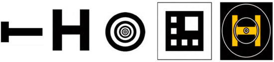
Figure 1.
Artificial markers.
Although the technology of autonomous landing for UAVs is relatively mature, in practical applications the UAVs need to work with a moving platform.
- (2)
- Autonomous Landing of UAVs in Dynamic Scenes
While performing complex tasks, UAVs need to collaborate with moving platforms. Compared with static scenes, landing in dynamic scenes is harder and the complexity of the technology is much higher, which necessitates the need to improve the control and navigation systems of UAVs. Meanwhile, the mission objectives of the two types of landing are almost the same, which means the autonomous landing methods mentioned above in static scenes are also widely used in dynamic scenes. Li proposed a Bi-directional Long and Short-Term Memory (Bi-KSTM) neural network for predicting the attitude of an unmanned boat, designed a PID controller, and achieved attitude synchronization between the UAV and the USV during autonomous landing [17]. Khazetdinov uses visual sensors to design embedded ArUco markers (e-ArUco), enabling landing using only the ArUco algorithm in a Gazebo simulation platform. The experimental results showed an average landing precision of 2.03 cm with a standard deviation of 1.53 cm [18]. In Lin’s study, Lin proposed a novel vision system that integrates infrared imaging technology and deep learning algorithms, aiming to enhance both accuracy and robustness. The experimental results demonstrate the method’s reliability [19]. Zhang designed an adaptive learning navigation rule with multiple layers, determining the position of the unmanned boat and achieving horizontal tracking and vertical descent of the UAV based on position feedback [20]. Table 1 is a further organization of the relevant work over the past five years. From the experimental results, although Jiang and his team [21] achieved 100% success, they did not validate the experimental algorithm on a real UAV. Moreover, their simulation environment was overly simple, giving the algorithm a higher fault-tolerance. While Neves et al. [22] demonstrated strong innovation and achieved good results, their method relies on high-performance GPUs. This dependency may limit the method’s application in resource-constrained environments. Chen’s team [23] used a complex model to achieve up to 98% accuracy. However, this boosted performance also raised computational demands, requiring high-end hardware and making it unsuitable for lightweight UAVs. In Dong et al.’s study [24], the UAV integrated multiple sensors, which increased its payload. The UAV achieved 100% success only on a slow-moving (0.5 m/s) target platform, as stated in the paper.

Table 1.
The relevant work over the past five years.
While the technology for autonomous landings is relatively mature, there is still a lot of room for development in the dynamic landing of UAVs. In this paper, we divided the process of autonomous landing into three main parts: target platform localization, trajectory tracking in fixed height, and final autonomous landing. The first part proposed a generic positioning method for the UAV to achieve real-time localization of the target platform. The second part simplified the Motion Planning and Control Controller (MPC) to enable the UAV to track the target landing platform on a horizontal plane while maintaining a constant altitude. The third part designed nested Apriltags cooperative markers and combined them with a PID speed controller using a Intel RealSense Depth Camera D435 (Intel, Santa Clara, CA, USA) for real-time tracking of the cooperative markers, enabling the UAV to complete autonomous landing. This method is not constrained by UAV computing resources and can be deployed in diverse real-world scenarios. The comprehensive technical flowchart for the UAV’s autonomous landing process is presented in Figure 2.
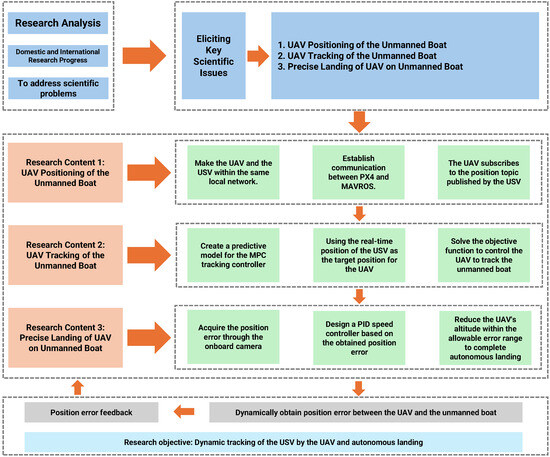
Figure 2.
UAV autonomous landing technical flowchart.
2. Modeling and Experimental Platform Specifications
In this section, we introduce the mathematical model of the UAV, the simulation platform, and physical platform specifications.
2.1. UAV Modeling
For the study of collaborative landing between UAVs and USVs, first, a mathematical model for the UAV must be established [25]. This study employs an X-type UAV as the research subject. The UAV is assumed to be a rigid and symmetric structure with its center of mass located at its geometric center. To describe the UAV’s position and attitude, we define the earth-centered inertial reference frame OE-XEYEZE and the body-fixed frame OB-XBYBZB, as shown in Figure 3.
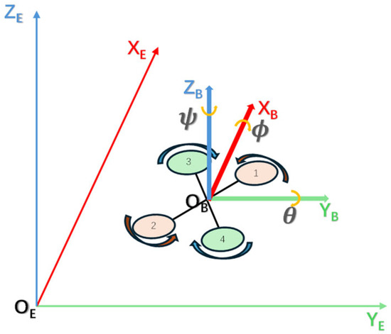
Figure 3.
Body-fixed frame and earth-centered inertial reference frame. 1–4 represent the UAV’s four motors. Motors 1 and 2 have the same rotation direction, as do motors 3 and 4.
The lift of the four-rotor UAV is generated by the rapid rotation of its four propellers. By adjusting the rotational speeds of the four motors, the position and attitude of the four-rotor UAV can be controlled. Based on the illustration provided in Figure 3, the mathematical model of the UAV is as follows:
In the above equations: are the rotational angles of the body around the y-axis, x-axis, and z-axis. and are the rotational inertia of the body in three axes (x, y, z). are the coefficients of air resistance.
,, , , and are given by the following equation:
are the speeds of the four motors.
2.2. Relative Motion
It is necessary to consider the kinematic issues of the relative motion between the UAV and the USV. We define as the position vector of the drone in the inertial coordinate system and as the position vector of the USV in the inertial coordinate system.
is the relative position of the drone and the USV.
UAV translational dynamics:
USV translational dynamics:
In formula (5), is the thrust of the unmanned ship. is the steering angle. are linear damping factors. According to the above formula, we can get the relative dynamics formula of UAV and USV.
2.3. Simulation Environment
ROS1 (Robot Operating System) under Ubuntu 20.04 is an open-source framework designed for robot operation systems, providing developers with a robust set of tools and APIs to build and control automated robotic systems. At its core, ROS incorporates three fundamental concepts: nodes, services, and topics. Nodes operate similarly to system processes, enabling developers to publish or subscribe to information flows; services, on the other hand, provide asynchronous functionality by allowing clients to request responses from remote or local servers; topics represent real-time data streams, facilitating dynamic event notifications in complex environments. These architectural components collectively enable robots to interact efficiently and perform operations within their operational environment.
The experiment utilized MAVROS and PX4 for joint simulation on the Gazebo platform. MAVROS is an officially provided tool under ROS that receives and sends MAVLink messages. Using MAVROS allows sending MAVLink messages to the flight control system and receiving data from it. The communication relationship between ROS and PX4 is illustrated in Figure 4.
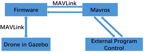
Figure 4.
Communication graph between ROS and PX4.
By writing code in ROS, subscribing to or publishing MAVROS topics, subscribing to the drone’s state, and publishing the expected position or expected speed of the drone, PX4 flight control can track the expected motion.
2.4. Physical Platform Specifications
To verify the autonomous landing algorithm of the UAV, we assembled an F450 UAV, as shown in Figure 5. The UAV employs an Orangepi5b as the onboard computer, which is equipped with the Ubuntu 20.04 system. By configuring ROS, PX4, and MAVROS, we can conduct secondary development on the UAV. We use the D435 camera as the downward camera to recognize Apriltags identifiers.
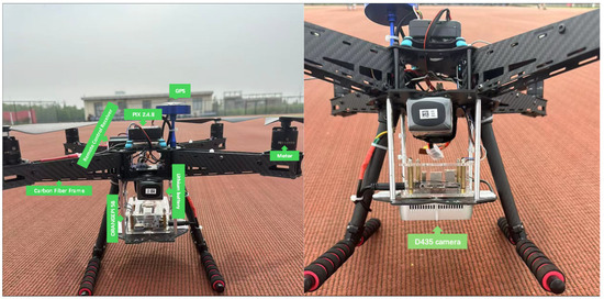
Figure 5.
The structure of the UAV.
3. Research Methods
3.1. Positioning Phase
This experiment is based on ROS + PX4 + MAVROS + Gazebo joint simulation, and the UAV control node needs to subscribe to the position topic of the mobile platform to obtain the position of the mobile platform as shown in Figure 6. The node diagram is illustrated in Figure 7.
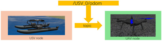
Figure 6.
The topic communication between the UAV and USV.
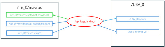
Figure 7.
UAV and USV node diagram.
In Figure 6, the apriltag_landing node represents the UAV’s motion control node. It subscribes to the odometry topic ugv_0/odom from the USV, enabling the UAV to receive real-time position and velocity information of the USV. The information is subsequently published through mavros-related publisher topics to facilitate position and attitude control of the UAV, thereby achieving localization and tracking of the USV by the UAV.
3.2. The Tracking Phase
After the UAV acquires the position information of the USV, it employs an MPC to enable the UAV to track the USV. The UAV first flies to a fixed altitude, and then tracks the trajectory of the unmanned boat in the XY plane. This enables the UAV to quickly fly to the vicinity of the USV, ensuring that the downward-facing camera on the UAV can identify the Apriltags markers on the USV. Tracking the unmanned boat in the XY plane at a fixed altitude simplifies the complexity of the MPC, transforming the UAV’s motion control in three-dimensional space into motion control in two-dimensional space. Figure 8 illustrates this configuration.
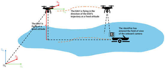
Figure 8.
Illustration of the tracking phase. The dashed black line indicates the UAV and USV positions in the Earth coordinate system. The dashed orange line shows the trajectory the UAV needs to follow for the USV.
The predictive model forms the basis of MPC, enabling it to predict future system responses based on control actions. This capability enables the controller to utilize real-time states and operational constraints to forecast system dynamics over a specified prediction horizon, thereby optimizing control inputs to achieve desired system performance.
The UAV dynamics model is based on rigid body kinematics and Newton–Euler equations, and the state variables are defined as:
Among them, x, y, z represent the UAV’s position, , , represents the UAV’s velocity, r, p, represent the roll, pitch, and yaw angles of the UAV, respectively, and , , represent the angular velocity.
The nonlinear dynamics equations are:
When the UAV is hovering or moving at low speed, the attitude angles involved in the UAV’s motion can be linearized: , , , , , , , . By removing the disturbance terms, the predictive model is further simplified to obtain Equation (8).
Linearization using the Jacobian matrix near the hover equilibrium point:
In the above formula, , . The continuous state–space model obtained after linearization is:
The positions and yaw angles are extracted through the output matrix . So . We use a zero-order hold (ZOH) for discretization with a sampling period of . The discrete equation is as follows:
In the prediction horizon , the state prediction equation is:
is the state prediction matrix. is the control input matrix. is the state transition matrix.
is the free response matrix.
To minimize the tracking error and the cost of control inputs, the objective function is constructed
In the above formula, and are the weight matrices. Since the control input simulates the analog signal of a remote controller, the control input has the following constraints:
After transforming the objective function into the standard quadratic form, the following equation is obtained:
In the above formula, By solving the above QP problem, the first control input obtained from the solution is applied to the UAV, and the state is updated.
3.3. Landing Phase
During the UAV landing phase, we designed a UAV PID speed controller based on the position error obtained by the downward-facing camera. Meanwhile, to ensure that the UAV can land stably in a windy environment, we conducted wind resistance tests on the UAV. First, we tested the algorithm in a simulation environment, as shown in Figure 9, and then validated the algorithm again by deploying it on a real UAV.
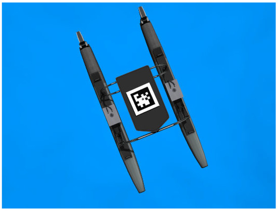
Figure 9.
USV equipped with Apriltags markers in Gazebo.
3.3.1. Multi-Apriltag Marker-Based Design
During the UAV landing process, as the altitude gradually decreases, the field of view of the camera continuously shrinks. When the UAV descends to a certain altitude, the camera can no longer identify the complete identifier. As shown in Figure 10, a single marker cannot meet the precision requirements for the unmanned aircraft’s accurate landing.
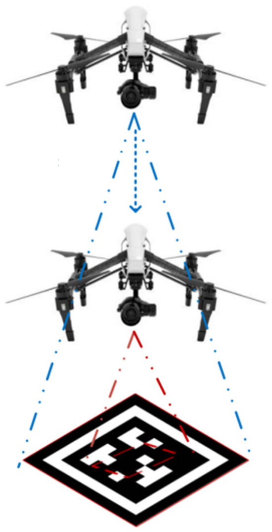
Figure 10.
Overlapping vision range diagram. As the UAV lands, the identifier recognition area shifts from the blue dashed line to the red dashed line.
To address the problem mentioned above, we designed a cooperative identifier [26,27]. As shown in Figure 11. When the UAV is at a higher altitude, it recognizes the larger external marker. When the altitude of the UAV gradually decreases and it can no longer recognize the complete external marker, the UAV begins to recognize the internal marker. To achieve precise landing, a large empty space should be maintained in the center of the external marker. In this experiment, the TAG36H11 family member with ID 236 was selected as the large-sized Apriltag marker, while the ID 2 Apriltag marker was used for small-sized object marker.
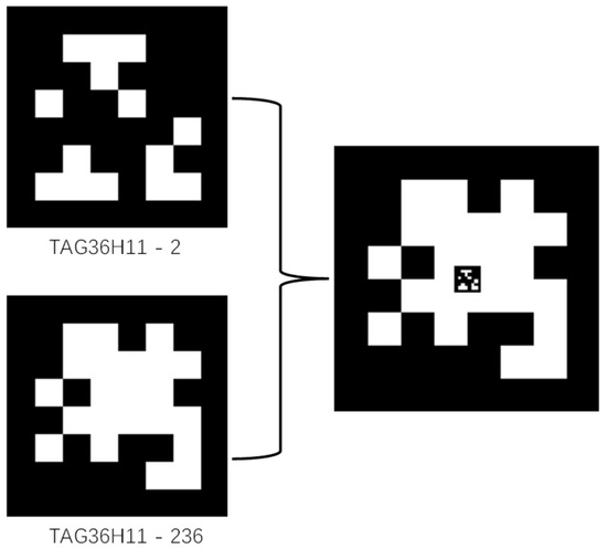
Figure 11.
Embedded Apriltag markers.
3.3.2. Design of the PID Speed Controller
We designed a PID speed controller based on the position error obtained from the Apriltags algorithm under the ROS platform to enable the UAV to track the marker. The Apriltags algorithm’s subscription and publication of messages is illustrated in Figure 12.
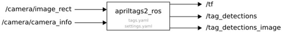
Figure 12.
Apriltag algorithm’s node information in ROS.
At the UAV control node, the position of the camera relative to the center of the identifier is obtained by subscribing to the /tag_detections topic.
The relative position obtained is used as the error input for the PID controller to obtain the control input of the UAV speed controller, as shown in Figure 13. When the UAV is tracking, a permissible landing error range is set. When the relative position between the UAV and the identifier is within the error range, the UAV completes the autonomous landing by gradually reducing its altitude.
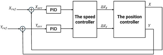
Figure 13.
The PID speed controller. This experiment uses PX4 firmware for simulation, where PX4 employs cascade control with an inner loop for speed PID control and an outer loop for position proportional control.
3.4. Aerodynamic Disturbances
During the flight process, the UAV is aways affected by wind. In order to enable the UAV to complete autonomous landing under the influence of wind, we conducted simulation experiments on the wind resistance capability of UAVs. Based on the existing wind field model [28] and in combination with the UAV dynamics model, we design a composite controller to allow the UAV to complete the landing task.
3.4.1. Wind Field Model
The wind speed model proposed in this paper is based on the following assumptions: The wind speed consists of a constant wind speed part and a dynamically changing gust part. The constant wind speed part represents the basic level of wind speed, while the gust part reflects the random fluctuations of wind speed. By introducing a time decay factor and random disturbances, the model can more accurately simulate the dynamic changes in wind speed.
The mathematical expression of the model is as follows:
represents the constant wind speed, and the is the gust. The gust is composed of the decaying gust and the random gust. The expression is as follows:
The refers to the last gust speed, and the exponential decay function is introduced to simulate the attenuation of the wind. In Equation (20), the represents the strength of turbulence. The function generates a random vector of length 3, which simulates the random fluctuations of wind speed in three directions. The variable is the time decay factor, used to simulate the decaying characteristics of random gusts over time.
3.4.2. Wind Resistance Control System
Based on the wind force model and the UAV dynamics model, we designed the UAV control system to achieve wind resistance. The controller included two main parts: the PID controller and the DOB (Disturbance Observer).
The PID controller is used to realize position tracking and the discrete PID controller is as follows:
is the input vector and is the position error vector caused by wind; the proportional part can generate a control force to counteract wind force in real time. The differential part can predict the trend of error change and provide damping in advance to counteract the oscillations caused by wind. The integral part can accumulate deviations caused by wind. To prevent integral windup, the integral term is limited to the range (−5, +5). Due to the limited thrust of the UAV, the output of the PID controller is constrained within the range of (−15, +15).
The DOB can estimate and provide feedforward compensation for external disturbances in real time. The mathematical expression of the disturbance observer is as follows:
The is the sensitivity of the control observer to the error. The is the actual acceleration of the UAV. The u is the control force currently output by the PID controller, so it can be inferred that is the theoretical acceleration. is the currently estimated disturbance wind force.
The mathematical formula of this control system is as follows:
In this way, we can maintain the simplicity of PID while significantly enhancing wind resistance performance through the disturbance observer.
4. Results
In this section, we discuss the experimental results of the simulation and the real UAV.
4.1. MPC Tracking Controller Results Display
In this section, we use MATLAB R2023a to evaluate the results of the MPC trajectory tracking controller. Since the USV is affected by waves during its movement, it often has difficulty moving in a straight line. Therefore, a circular trajectory is adopted for the USV. The tracking performance is shown in Figure 14, where the red solid line represents the trajectory of the USV and the blue solid line represents the trajectory of the UAV.
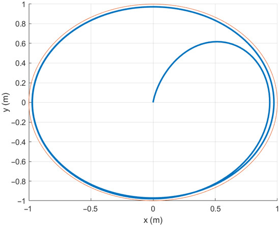
Figure 14.
The unmanned aircraft tracks a circular path. The red solid line is the reference trajectory, and the blue solid line is the UAV’s trajectory.
Figure 15 and Figure 16 illustrate the UAV’s trajectory tracking in X and Y directions. Figure 17 and Figure 18 depict the tracking errors in X and Y directions, respectively. The results indicate that the errors in both X and Y directions remain within the range of −0.8 to 0.8 during the tracking process. Figure 19 shows the ability of the UAV to track the yaw angle of the USV, and the UAV can quickly perform this tracking task.
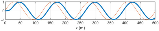
Figure 15.
A trajectory tracking diagram in the X-direction. The red solid line is the reference trajectory in the X-direction, and the blue solid line is the UAV’s trajectory in the X-direction.
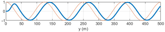
Figure 16.
A trajectory tracking diagram in the Y-direction. The red solid line is the reference trajectory in the Y-direction, and the blue solid line is the UAV’s trajectory in the Y-direction.
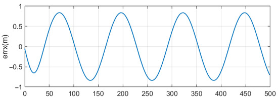
Figure 17.
The X-direction tracking error curve. The UAV’s error in the X-direction ranges from −0.8 to 0.8.
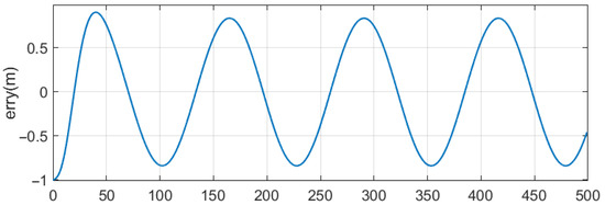
Figure 18.
The Y-direction tracking error curve. The UAV’s error in the Y-direction ranges from −0.8 to 0.8.
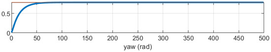
Figure 19.
A trajectory diagram for unmanned aircraft pitch angle tracking. The UAV completes tracking in the z-direction after step 50 of the simulation.
Based on the results presented, the tracking phase demonstrates that the UAV can effectively track the autonomous vessel and meet the requirements for the landing stage.
4.2. Landing Phase PID Controller Analysis and Results Demonstration
In the landing phase, we verified the effectiveness of the PID speed controller by having the UAV track both straight and circular trajectories.
The general form of the PID controller is as follows:
After obtaining the relative position of the onboard camera with respect to the barcode, the camera coordinate system follows the right-hand coordinate system. Therefore, the X direction of the downward-looking camera corresponds to the Y direction of the UAV, and the Y direction corresponds to the X direction of the UAV. An error identified in the X direction is noted as . The PID controller for the X direction is as follows:
Similarly, the PID controller for the Y direction is as follows:
We have tuned the controller parameters using the Ziegler–Nichols method. The PID controller parameters for the X and Y directions are as shown in Table 2.
Table 2.
PID controller parameters table for X and Y directions.
According to Equation (1), the horizontal position dynamics of the UAV can be expressed as:
Since the UAV does not consider air resistance in the simulation environment and the changes in the UAV’s body angle during the tracking process are small, the above formula can be simplified as:
Taking the Laplace transform of the above formula yields:
The transfer function in the Y direction has the same form as that in the X direction.
The transfer function of the PID controller is:
The closed-loop transfer function of the system is:
According to the Routh stability criterion, the system is stable.
Figure 20 illustrates the line tracking error graph of the UAV controlled by the PID controller for the USV. The Y-direction error is within the range of −0.8 to 0.8. The X-direction error increases with the speed of the USV. As shown, when the USV moves at 1.8 m/s, the error between the UAV and the Apriltag marker is approximately 2 m. This fails to meet the landing conditions, hence an improvement of the PID controller is required.
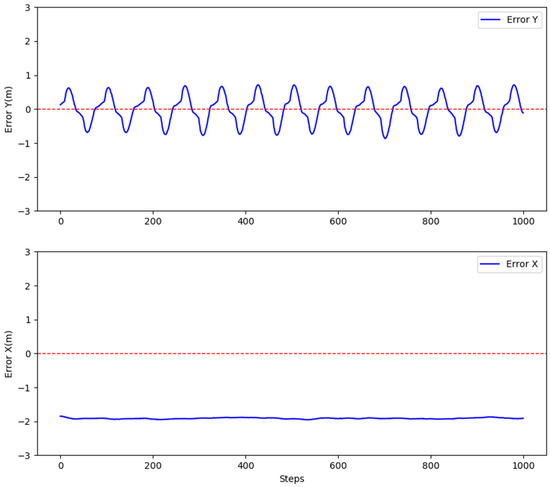
Figure 20.
Illustration of UAV’s tracking error for straight trajectory. The UAV here uses an unmodified PID velocity controller.
This experiment improves the precision of autonomous landing of the UAV by adding bias terms to the PID controller. The PID controller with added bias terms is as follows:
This bias term, , represents the speed of the moving platform in the X-direction. By increasing the bias term , we can reduce the tracking error for the target markers.
Similarly, the PID controller for the Y direction is as follows:
The trajectory of the line tracking, as shown in Figure 21, illustrates the drone’s movement along the x-axis. The target moving platform moves at a speed of 3 m/s along the x-axis. The UAV’s y-axis error ranges from −0.8 m to 0.8 m, while the x-axis error ranges from −0.4 m to 0.4 m. When the errors in both the X and Y directions are within the range of (−0.3, 0.3) meters, the UAV will gradually reduce its altitude to complete the autonomous landing. Otherwise, it will continue to track at the current altitude until the autonomous landing is accomplished. The error illustration is shown in Figure 22.
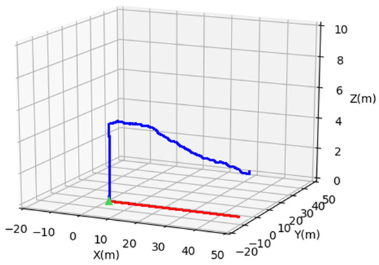
Figure 21.
The line tracking illustration of the UAV’s autonomous landing. The green triangle denotes the initial positions of the UAV and USV. The red solid line shows the USV’s trajectory, while the blue solid line represents the UAV’s trajectory.
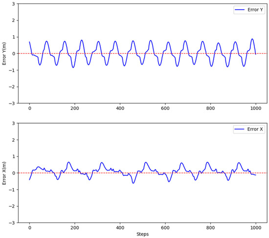
Figure 22.
Unmanned aerial vehicle (UAV) tracking of Apriltags markers for straight trajectory error diagram. The UAV here uses the improved PID velocity controller. Thank you for pointing out the issue.
Due to the influence of wind and waves on the USV, it is typically difficult for the USV to maintain straight-line movement, necessitating experiments on nonlinear trajectories. Figure 23 illustrates the trajectory tracking illustration of the drone when following a circular path by the USV moving at a speed of 2 m/s with angular velocity of 0.15 rad/s. When the drone identifies Apriltag markers, it performs height reduction if both X and Y directional errors are within −0.3 to 0.3 m. As shown in Figure 24, the X-direction error is between −0.4 to 0.4 m and the Y-direction error is between −0.4 to −0.2 m. Once the drone’s landing conditions are met, it lowers its height at a rate of −0.2 m/s in the Z-axis to complete the landing.
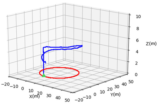
Figure 23.
UAV tracking of Apriltag markers for circular trajectory. The green triangle denotes the initial positions of the UAV and USV. The red solid line shows the USV’s trajectory, while the blue solid line represents the UAV’s trajectory.
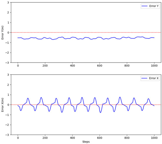
Figure 24.
Unmanned aerial vehicle (UAV) tracking of Apriltags markers for circular trajectory error diagram.
The experimental results indicate that when the USV moves at a speed of 3 m/s, the UAV’s X-direction error ranges between −0.5 and 0.5 m, while the Y-direction error ranges between −0.8 and 0.8 m, satisfying the landing conditions. Additionally, during the circular trajectory tracking process, when the USV moves at a speed of 2 m/s (v) and an angular speed of 0.2 rad/s (ω), the UAV’s X-direction error is within the range of −0.4 to 0.4 m, while the Y-direction error remains between −0.4 and −0.2 m. The experimental results demonstrate that the proposed method can satisfy the requirement for UAV landing on a dynamic platform.
4.3. The Results of Wind Force Simulation
In this section, we will analyze the simulation results of the controller based on the data obtained from the simulation.
To begin with, we will provide the initial values of the PID controller parameters and the tuning criteria.
- Proportional gain :
Based on empirical formulas, the initial value of is
is the desired settling time. The target position is (10, 15, 5), and the desired time is set to 5. The mass of the UAV is 1.5 kg. We can get the = 0.96. A too-high can cause overshoot or oscillation, but a too-low will make the UAV respond untimely. The final experimental results show that = [3, 3, 4].
- Differential gain :
We set the system damping ratio to 0.7. The initial value of is
is the drag coefficient, which is used to quantify the effect of air resistance on the UAV during its motion. Since the current experiment uses a small quadrotor UAV, is set to 0.2. We can get the = 1.48. The final experimental results show that = [1.5, 1.5, 2].
- Integral gain :
The initial value of the integral gain should be much smaller than .
is the dominant time constant of the system. The initial value of is usually between one-third and one-half of the settling time, which is considered optimal. Therefore, we take as 2. We can get the . The final experimental results show that = [0.1, 0.1, 0.2].
The UAV dynamics model is a second-order system, and the open-loop transfer function is:
The closed-loop transfer function after introducing proportional, integral, and differential terms is:
The closed-loop system is proven to be stable using the Routh stability criterion.
We conducted experiments under the following wind field parameters: (X:2, Y:1.5, Z:1); (X:6, Y:7, Z:8); (X:11.5, Y:12.5, Z:12). The simulation results are shown in Figure 25, Figure 26 and Figure 27. When the wind force is relatively small, the UAV can respond quickly and reach the target position in a short time. However, as the wind force gradually increases, the overshoot of the UAV in the X and Y directions will continue to increase. But according to the results, the UAV can still fly to the designated position. Therefore, the controller can enable the UAV to have certain wind resistance capabilities.
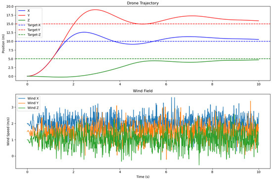
Figure 25.
The simulation results when the wind field parameters are {X:2, Y:1.5, Z:2}.
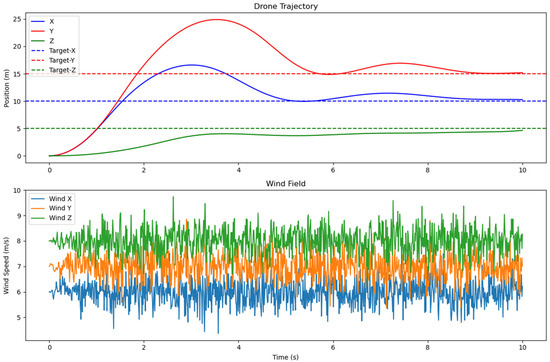
Figure 26.
The simulation results when the wind field parameters are (X:6, Y:7, Z:8).
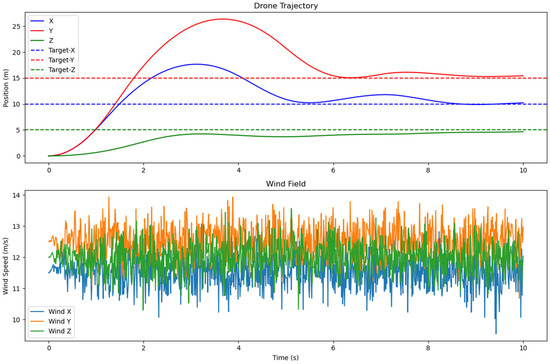
Figure 27.
The simulation results when the wind field parameters are (X:11.5, Y:12.5, Z:12).
5. Conclusions and Future Works
This paper divides the UAV landing process into three stages: positioning, tracking, and landing. Each stage is validated in the paper, which enhances the efficiency of UAV autonomous landing. Simultaneously, the UAV is tested for wind resistance through simulation.
Here it needs to be explained that since the MPC controller in the experiment requires control of the UAV’s torque, and MAVROS has a very poor effect on torque control, we used MATLAB for simulation during the tracking phase. Based on the simulation results, the MPC performs as expected during the tracking phase, but it still needs to be verified in real UAVs.
In the final landing phase, the algorithm from the simulation was transferred to a real UAV for algorithm validation. The experimental results are similar to the simulation results, capable of completing the landing task with a success rate of over 90%. It needs to be explained that, due to the limitations of the experimental conditions, we used manual dragging of a homemade identifier to simulate the movement of the unmanned boat. Therefore, it is not possible to fully replicate the motion of the unmanned boat on the water.
At this stage, we have achieved UAV autonomous landing on dynamic platforms, but some issues remain to be resolved. In our experiments, the UAV and USV must share position information over a local area network. Network instability can lead to data loss, thereby delaying the UAV’s response. Compared to other teams [22,23,24], we may need to add sensors like LiDAR to improve the final landing accuracy. When conducting the wind resistance experiments for UAVs, there are still some shortcomings when compared with those of other researchers [29].
In future work, to prevent UAVs from being affected by network instability, we may improve the UAV’s positioning method for target moving platforms. Additionally, to ensure final landing accuracy, we will consider adding sensors to the UAV. However, the main focus will remain on optimizing the UAV’s control algorithm.
Author Contributions
Conceptualization, Y.L. and R.L.; methodology, R.L.; software, R.L. and Y.L.; validation, R.L.; formal analysis, R.L. and J.W.; investigation, Y.L. and R.L.; resources, Y.L. and R.L.; data curation, R.L. and J.W.; writing—original draft preparation, R.L. and Y.L.; writing—review and editing, R.L. and Y.L.; visualization, R.L. and J.W.; supervision, Y.L.; project administration, Y.L. and R.L.; funding acquisition, Y.L. and R.L. All authors have read and agreed to the published version of the manuscript.
Funding
This research received no external funding.
Data Availability Statement
The data that support the findings of this study are available from the corresponding author upon reasonable request.
Conflicts of Interest
The authors declare no conflicts of interest.
References
- Fan, B.; Li, Y.; Zhang, R.; Fu, Q. Review on the technological development and application of UAV systems. Chin. J. Electron. 2020, 29, 199–207. [Google Scholar] [CrossRef]
- Muchiri, G.; Kimathi, S. A review of applications and potential applications of UAV. In Proceedings of the Sustainable Research and Innovation Conference, Pretoria, South Africa, 20–24 June 2022; pp. 280–283. [Google Scholar]
- Tsouros, D.C.; Bibi, S.; Sarigiannidis, P.G. A review on UAV-based applications for precision agriculture. Information 2019, 10, 349. [Google Scholar] [CrossRef]
- Xiaoning, Z. Analysis of military application of UAV swarm technology. In Proceedings of the 2020 3rd International Conference on Unmanned Systems (ICUS), Harbin, China, 27–28 November 2020; pp. 1200–1204. [Google Scholar]
- Ma’Sum, M.A.; Arrofi, M.K.; Jati, G.; Arifin, F.; Kurniawan, M.N.; Mursanto, P.; Jatmiko, W. Simulation of intelligent unmanned aerial vehicle (UAV) for military surveillance. In Proceedings of the 2013 International Conference on Advanced Computer Science and Information Systems (ICACSIS), Sanur Bali, Indonesia, 28–29 September 2013; pp. 161–166. [Google Scholar]
- Utsav, A.; Abhishek, A.; Suraj, P.; Badhai, R.K. An IoT based UAV network for military applications. In Proceedings of the 2021 Sixth International Conference on Wireless Communications, Signal Processing and Networking (WiSPNET), Chennai, India, 25–27 March 2021; pp. 122–125. [Google Scholar]
- Xin, L.; Tang, Z.; Gai, W.; Liu, H. Vision-Based Autonomous Landing for the UAV: A Review. Aerospace 2022, 9, 634. [Google Scholar] [CrossRef]
- Alam, M.S.; Oluoch, J. A survey of safe landing zone detection techniques for autonomous unmanned aerial vehicles (UAVs). Expert Syst. Appl. 2021, 179, 115091. [Google Scholar] [CrossRef]
- Ariante, G.; Ponte, S.; Papa, U.; Del Core, G. Safe landing area determination (slad) for unmanned aircraft systems by using rotary lidar. In Proceedings of the 2021 IEEE 8th International Workshop on Metrology for AeroSpace (MetroAeroSpace), Naples, Italy, 23–25 June 2021; pp. 110–115. [Google Scholar]
- Liu, F.; Shan, J.; Xiong, B.; Fang, Z. A real-time and multi-sensor-based landing area recognition system for uavs. Drones 2022, 6, 118. [Google Scholar] [CrossRef]
- Raei, H.; Cho, Y.; Park, K. Autonomous landing on moving targets using LiDAR, Camera and IMU sensor Fusion. In Proceedings of the 2022 13th Asian Control Conference (ASCC), Jeju Island, Republic of Korea, 4–7 May 2022; pp. 419–423. [Google Scholar]
- Song, C.; Chen, Z.; Wang, K.; Luo, H.; Cheng, J.C. BIM-supported scan and flight planning for fully autonomous LiDAR-carrying UAVs. Autom. Constr. 2022, 142, 104533. [Google Scholar] [CrossRef]
- Yang, L.; Wang, C.; Wang, L. Autonomous UAVs landing site selection from point cloud in unknown environments. ISA Trans. 2022, 130, 610–628. [Google Scholar] [CrossRef] [PubMed]
- Jung, Y.; Lee, D.; Bang, H. Close-range vision navigation and guidance for rotary UAV autonomous landing. In Proceedings of the 2015 IEEE International Conference on Automation Science and Engineering (CASE), Gothenburg, Sweden, 24–28 August 2015; pp. 342–347. [Google Scholar]
- Saripalli, S.; Montgomery, J.F.; Sukhatme, G.S. Visually guided landing of an unmanned aerial vehicle. IEEE Trans. Robot. Autom. 2003, 19, 371–380. [Google Scholar] [CrossRef]
- Sharp, C.S.; Shakernia, O.; Sastry, S.S. A Vision System for Landing an Unmanned Aerial Vehicle. In Proceedings of the IEEE International Conference Robotics and Automation, Seoul, Republic of Korea, 21–26 May 2001. [Google Scholar]
- Tan, L.K.L.; Lim, B.C.; Park, G.; Low, K.H.; Yeo, V.C.S. Public acceptance of drone applications in a highly urbanized environment. Technol. Soc. 2021, 64, 101462. [Google Scholar] [CrossRef]
- Khazetdinov, A.; Zakiev, A.; Tsoy, T.; Svinin, M.; Magid, E. Embedded ArUco: A novel approach for high precision UAV landing. In Proceedings of the 2021 International Siberian Conference on Control and Communications (SIBCON), Kazan, Russia, 13–15 May 2021; pp. 1–6. [Google Scholar]
- Lin, S.; Jin, L.; Chen, Z. Real-time monocular vision system for UAV autonomous landing in outdoor low-illumination environments. Sensors 2021, 21, 6226. [Google Scholar] [CrossRef] [PubMed]
- Zhang, H.-T.; Hu, B.-B.; Xu, Z.; Cai, Z.; Liu, B.; Wang, X.; Geng, T.; Zhong, S.; Zhao, J. Visual navigation and landing control of an unmanned aerial vehicle on a moving autonomous surface vehicle via adaptive learning. IEEE Trans. Neural Netw. Learn. Syst. 2021, 32, 5345–5355. [Google Scholar] [CrossRef] [PubMed]
- Jiang, Z.; Song, G. A deep reinforcement learning strategy for UAV autonomous landing on a platform. In Proceedings of the 2022 International Conference on Computing, Robotics and System Sciences (ICRSS), Macau, China, 19–21 December 2022; pp. 104–109. [Google Scholar]
- Neves, F.S.; Branco, L.M.; Pereira, M.I.; Claro, R.M.; Pinto, A.M. A multimodal learning-based approach for autonomous landing of uav. In Proceedings of the 2024 20th IEEE/ASME International Conference on Mechatronic and Embedded Systems and Applications (MESA), Genova, Italy, 2–4 September 2024; pp. 1–8. [Google Scholar]
- Chen, L.; Xiao, Y.; Yuan, X.; Zhang, Y.; Zhu, J. Robust autonomous landing of UAVs in non-cooperative environments based on comprehensive terrain understanding. Sci. China Inf. Sci. 2022, 65, 212202. [Google Scholar] [CrossRef]
- Dong, X.; Gao, Y.; Guo, J.; Zuo, S.; Xiang, J.; Li, D.; Tu, Z. An integrated UWB-IMU-vision framework for autonomous approaching and landing of UAVs. Aerospace 2022, 9, 797. [Google Scholar] [CrossRef]
- Stepanov, V. Mathematical modelling of the unmanned aerial vehicle dynamics. Cucmeмный aнaлuз u пpuклaднaя uнфopмamuкa 2018, 1, 37–43. [Google Scholar] [CrossRef]
- Olson, E. AprilTag: A robust and flexible visual fiducial system. In Proceedings of the 2011 IEEE International Conference on Robotics and Automation, Shanghai, China, 9–13 May 2011; pp. 3400–3407. [Google Scholar]
- Wang, J.; Olson, E. AprilTag 2: Efficient and robust fiducial detection. In Proceedings of the 2016 IEEE/RSJ International Conference on Intelligent Robots and Systems (IROS), Daejeon, Republic of Korea, 9–14 October 2016; pp. 4193–4198. [Google Scholar]
- Phadke, A.; Medrano, F.A.; Chu, T.; Sekharan, C.N.; Starek, M.J. Modeling Wind and Obstacle Disturbances for Effective Performance Observations and Analysis of Resilience in UAV Swarms. Aerospace 2024, 11, 237. [Google Scholar] [CrossRef]
- Nordin, M.; Sharma, S.; Khan, A.; Gianni, M.; Rajendran, S.; Sutton, R. Collaborative Unmanned Vehicles for Inspection, Maintenance, and Repairs of Offshore Wind Turbines. Drones 2022, 6, 137. [Google Scholar] [CrossRef]
Disclaimer/Publisher’s Note: The statements, opinions and data contained in all publications are solely those of the individual author(s) and contributor(s) and not of MDPI and/or the editor(s). MDPI and/or the editor(s) disclaim responsibility for any injury to people or property resulting from any ideas, methods, instructions or products referred to in the content. |
© 2025 by the authors. Licensee MDPI, Basel, Switzerland. This article is an open access article distributed under the terms and conditions of the Creative Commons Attribution (CC BY) license (https://creativecommons.org/licenses/by/4.0/).