
Multi-UAV Trajectory Planning Based on a Two-Layer Algorithm Under Four-Dimensional Constraints


Abstract
1. Introduction
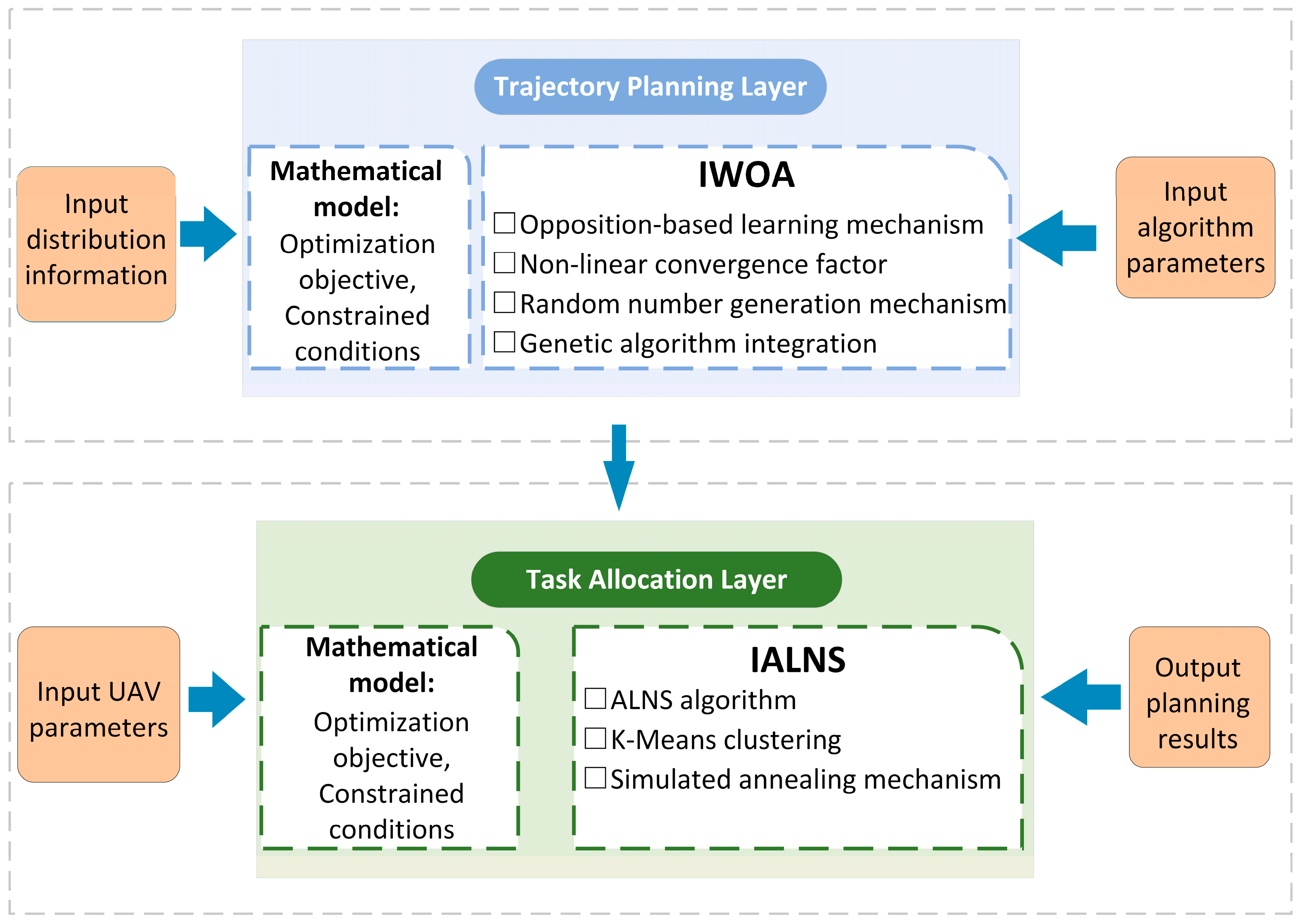
- A novel two-tier optimization framework is proposed to combine the improved adaptive large neighborhood search for global task allocation with the enhanced whale optimization algorithm for local trajectory planning to achieve coordinated scheduling in complex multi-UAV scenarios.
- Multi-dimensional constraints are integrated into a unified MDRP-TW formulation, and algorithmic components such as backward learning initialization, nonlinear convergence, and gene mutation are improved to enhance the stability and accuracy of the optimization.
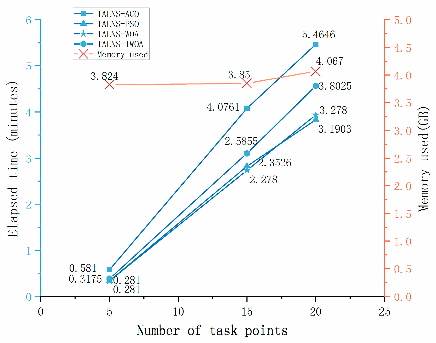
- The robustness and scalability of the proposed IALNS-IWOA framework is verified through many simulations under various task settings, and the superior performance is demonstrated in comparison with the baseline approaches such as IALNS-PSO, IALNS-WOA, and IALNS-ACO.
2. Modeling
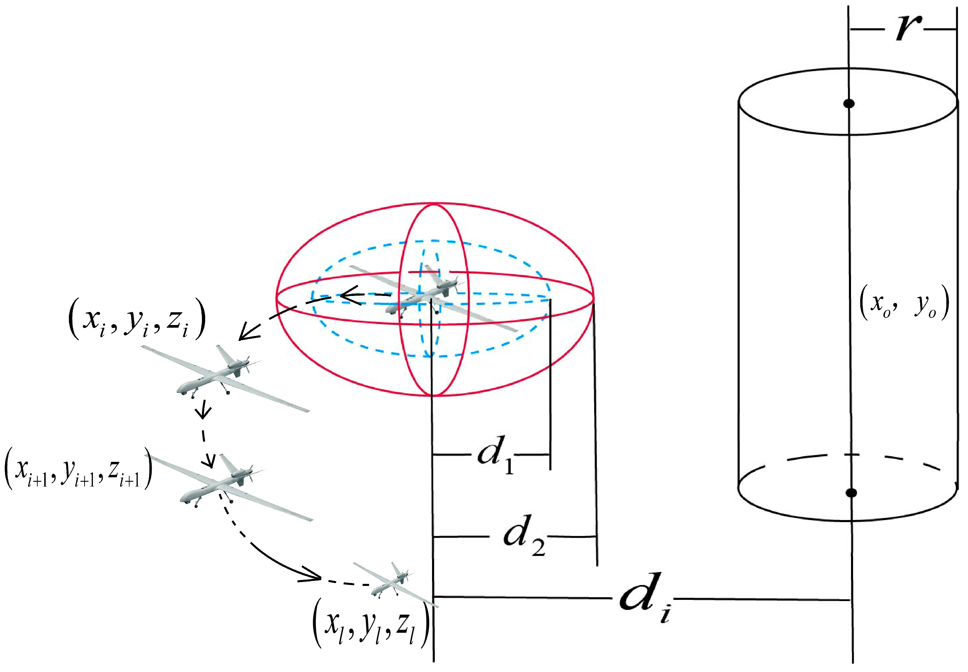
2.1. Mathematical Model of the Trajectory Planning Layer
2.2. Mathematical Model of the Task Allocation Layer
3. IALNS-IWOA Algorithm
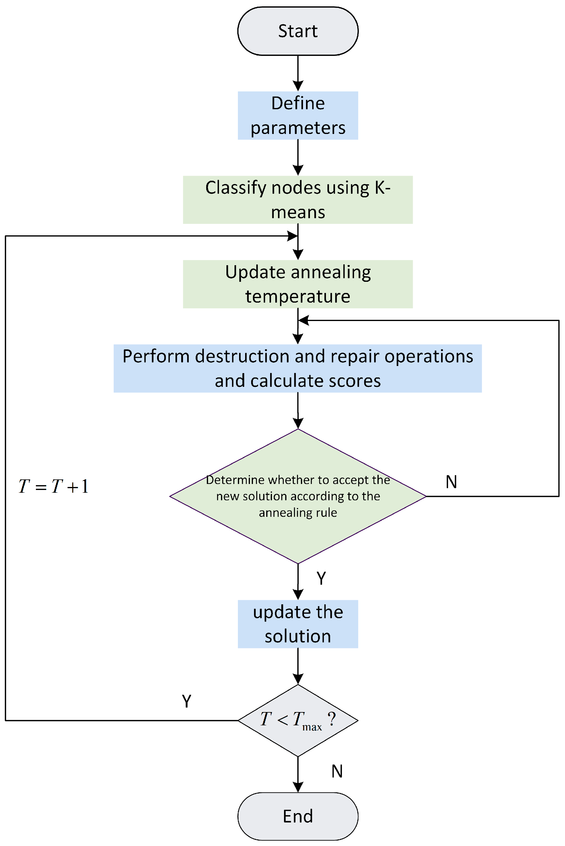
3.1. Adaptive Large Neighborhood Search
3.1.1. K-Means Clustering
3.1.2. Simulated Annealing Algorithm
| Algorithm 1: Adaptive large neighborhood search (IALNS) |
| 01: Input Clustering parameters; feasible initial solution from K-means clustering |
| 02:
;
;
; 03: Repeat 04: Update annealing temperature; update and ; select , ; 05: ; 06: Use the simulated annealing rule to determine whether to accept the new solution 07: If accepted, set ; 08: End if 09: Determine whether the new solution is accepted as the current best solution 10: If accepted, update and ; 11: End if 12: Until stopping criterion is met 13: Return the best solution |
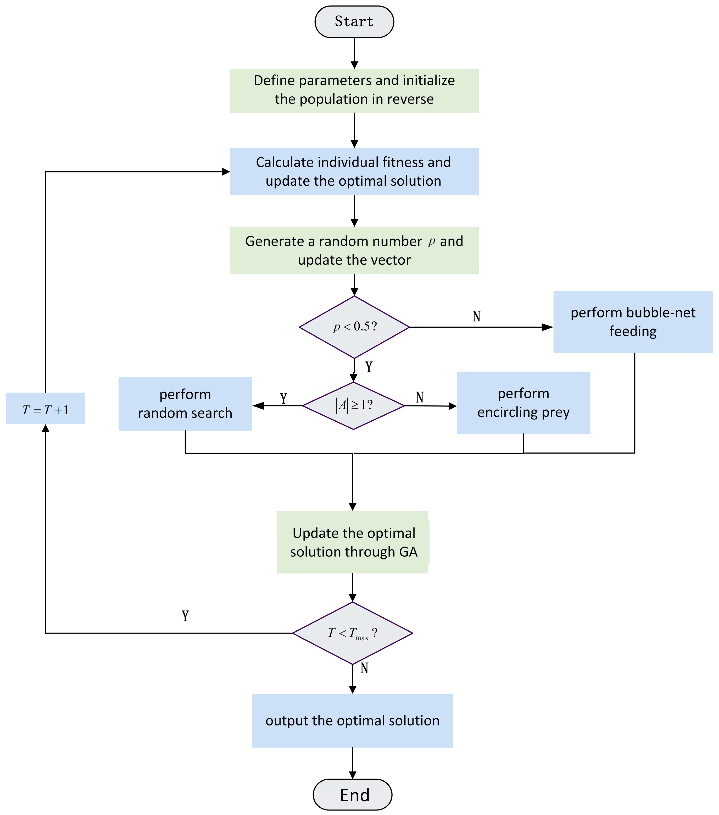
3.2. Improved Whale Optimization Algorithm
Genetic Algorithm
| Algorithm 2: Improved whale optimization algorithm (IWOA) |
| 01: Input Population size, maximum number of generations, search probability, variable range |
| 02: Execute reverse learning initialization to enhance population diversity 03: Evaluate the fitness value of each individual and determine the current best solution 04: Repeat 05 Calculate the nonlinear convergence factor and spiral coefficient 06 Generate a random number 07 If 08 If 09 Perform random search 10 Else: 11 Perform encircling prey 12 Else: 13 Update position using GA-based strategy 14 Update solution 15 End if 16 Determine whether termination condition is met 17 Return the best solution found |
4. Simulation Experiments
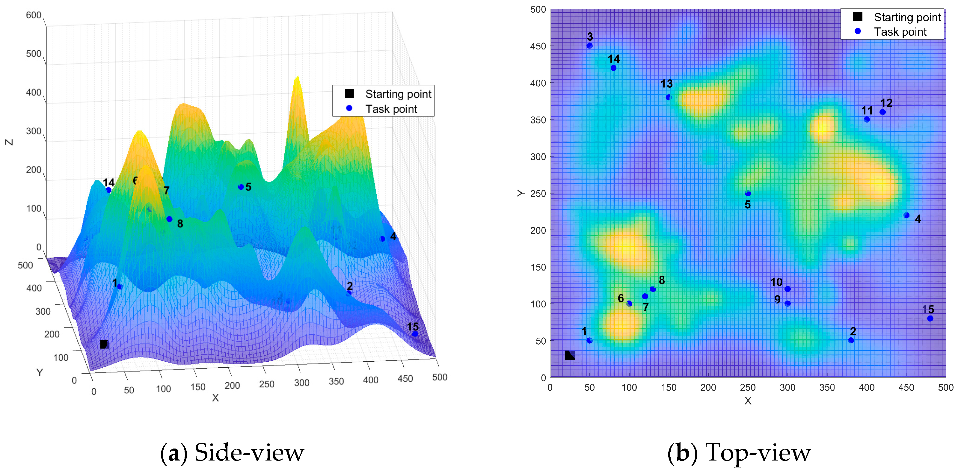
4.1. Simulation Environment and Mapping to Mathematical Model
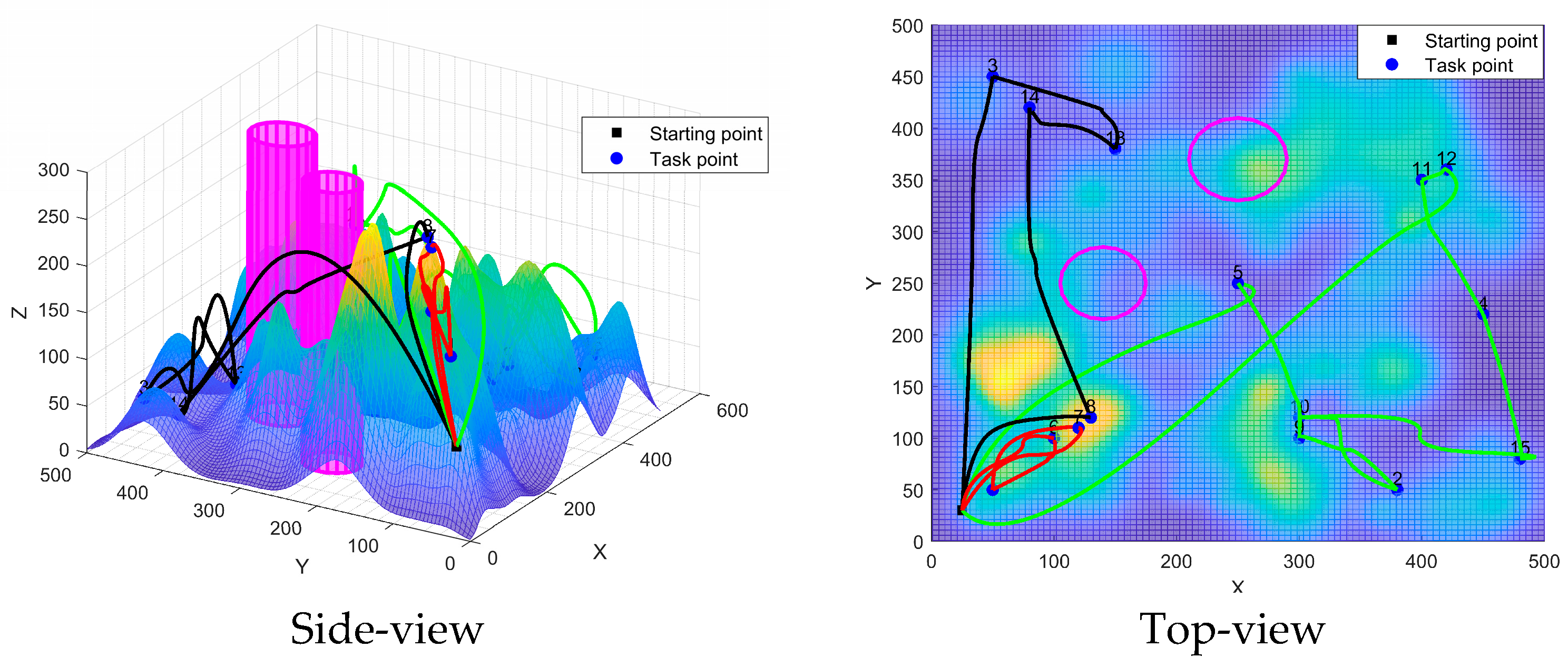
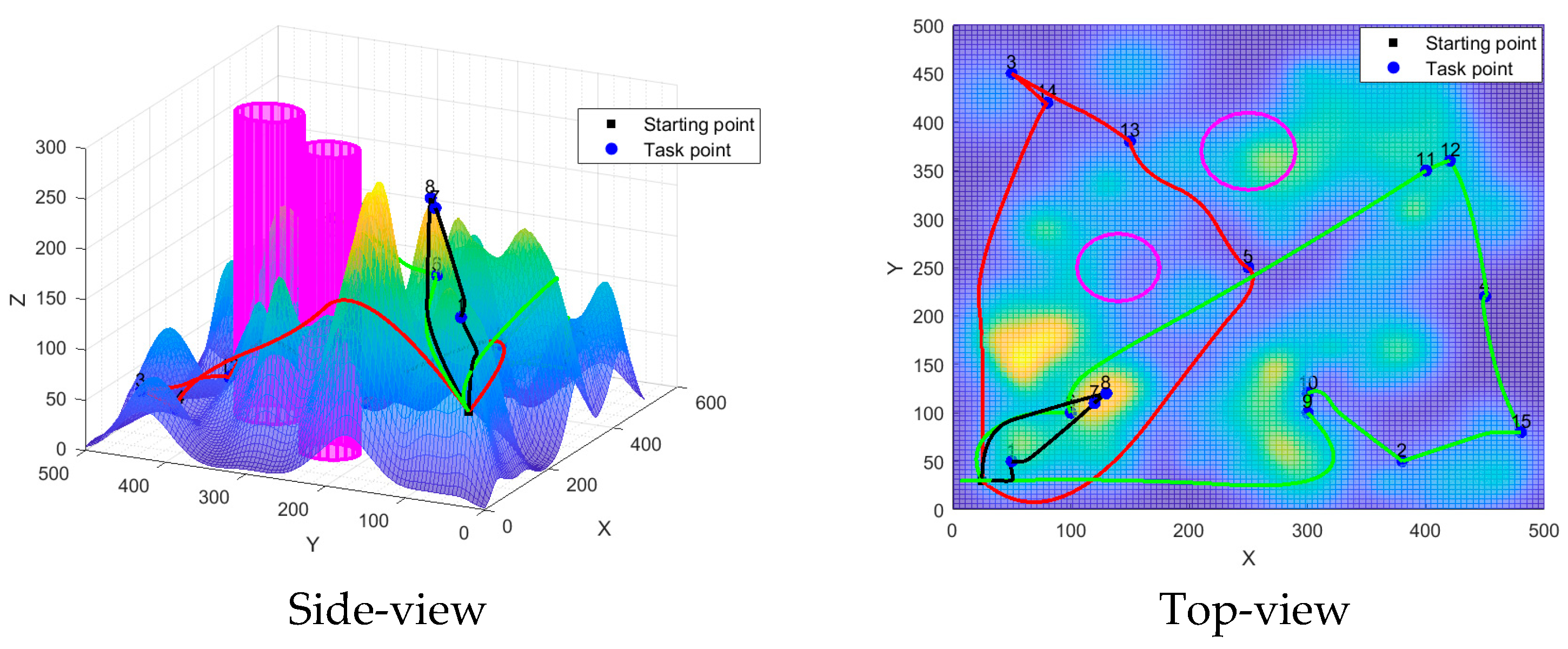
4.2. Experimental Results
4.2.1. Algorithm Base Performance Validation
4.2.2. Simulated Annealing Algorithm
4.2.3. Extended Experiments Under Varying Mission Scenarios
5. Future Research Directions
6. Conclusions
Author Contributions
Funding
Data Availability Statement
Conflicts of Interest
References
- The Chinese Communist Party (CCP) Central Committee; The State Council. China’s Foreign Economic Relations and Trade Bulletin. In Outline of the Strategic Plan for Expanding Domestic Demand (2022–2035); The Central Committee of the Communist Party of China and the State Council: Beijing, China, 2023; Volume 17, pp. 3–17. [Google Scholar]
- Li, H.; Wang, T.; Du, X. Analysis of collaborative navigation algorithms for multi-UAV swarm. Tactical Missile Technol. 2024, 6, 118–126. [Google Scholar]
- Fang, K.; An, Y.; Zhu, N.; Huang, D. The vehicle routing problem with drone stations. J. Manag. Sci. China 2025, 28, 61–76. [Google Scholar]
- Zhao, W.; Bian, X.; Mei, X. An Adaptive Multi-Objective Genetic Algorithm for Solving Heterogeneous Green City Vehicle Routing Problem. Appl. Sci. 2024, 14, 6594. [Google Scholar] [CrossRef]
- Pan, C. Research on Vehicle Routing Problem Based on Deep Reinforcement Learning. In Proceedings of the 2023 8th International Conference on Intelligent Computing and Signal Processing (ICSP), Xi’an, China, 21–23 April 2023; pp. 2116–2119. [Google Scholar]
- Huang, N.; Zhu, J.; Zhu, W.; Qin, H. The multi-trip vehicle routing problem with time windows and unloading queue at depot. Transp. Res. Part E Logist. Transp. Rev. 2021, 152, 102370. [Google Scholar] [CrossRef]
- Christian, M.M.F.; Alexander, J.; Markus, F.; Rainer, K. The vehicle routing problem with time windows and flexible delivery locations. Eur. J. Oper. Res. 2023, 308, 1142–1159. [Google Scholar]
- Liu, T.; Xu, W.; Wu, Q. Modeling of Multi-vehicle Route Searching with Soft Time Windows Under Sudden-on set Disaster. J. Tongji Univ. (Nat. Sci.) 2012, 40, 109. [Google Scholar]
- Zhang, L.; Wang, J.; Liu, X. Deep Reinforcement Learning for Dynamic Multi-UAV Path Planning in Urban Environments. IEEE Trans. Autom. Sci. Eng. 2024, 21, 712–725. [Google Scholar]
- Li, Y.; Chen, M.; Xu, J. A Hybrid GA-PSO Algorithm for Real Time Multi Drone Task Scheduling with Time Windows. J. Intell. Robot. Syst. 2023, 101, 34. [Google Scholar]
- Chen, Q.; Zhao, S.; Huang, H. Distributed Consensus Based Coordination for Heterogeneous UAV Swarms under Communication Constraints. Int. J. Robot. Res. 2025, 44, 58–75. [Google Scholar]
- Chen, R.; Li, J.; Chen, Y.; Huang, Y. A Distributed Scheduling Method for Networked UAV Swarm based on Computing for Communication. In Proceedings of the 2023 IEEE/RSJ International Conference on Intelligent Robots and Systems (IROS), Detroit, MI, USA, 1–5 October 2023; pp. 11071–11078. [Google Scholar]
- Kim, S.; Lee, H. Real time Obstacle Avoidance for Multi UAV Systems Using Graph Neural Networks. J. Field Robot. 2024, 41, 295–312. [Google Scholar]
- Sato, Y.; Tanaka, K.; Watanabe, M. Multi Agent Reinforcement Learning and Game Theoretic Co-ordination for UAV Airspace Sharing. In Proceedings of the International Conference on Intelligent Unmanned Systems, Changzhou, China, 18–19 September 2025; Volume 12, pp. 88–97. [Google Scholar]
- Jonas, W.; Julius, R.; Marija, P. Multi-UAV Adaptive Path Planning Using Deep Reinforcement Learning. In Proceedings of the IEEE/RSJ International Conference on Intelligent Robots and Systems (IROS), Detroit, MI, USA, 1–5 October 2023; pp. 649–656. [Google Scholar]
- Tang, J.; Liang, Y.; Li, K. Dynamic Scene Path Planning of UAVs Based on Deep Reinforcement Learning. Drones 2024, 8, 60. [Google Scholar] [CrossRef]
- Li, Y.; Hamid, A.A.; Dong, D. Path Planning for Cellular-Connected UAV: A DRL Solution With Quantum-Inspired Experience Replay. IEEE Trans. Wirel. Commun. 2022, 21, 7897–7912. [Google Scholar] [CrossRef]
- Li, Y.; Aghvami, A.H.; Dong, D. Intelligent Trajectory Planning in UAV-Mounted Wireless Networks: A Quantum-Inspired Reinforcement Learning Perspective. IEEE Wirel. Commun. Lett. 2021, 10, 1994–1998. [Google Scholar] [CrossRef]
- Xu, Y.; Wei, Y.; Jiang, K.; Wang, D.; Deng, H. Multiple UAVs Path Planning Based on Deep Reinforcement Learning in Communication Denial Environment. Mathematics 2023, 11, 405. [Google Scholar] [CrossRef]
- Hans, H.; Dirk, H.; Felix, W.; Rank, K. Quantum Deep Reinforcement Learning for Robot Navigation Tasks. IEEE Access 2022, 12, 87217–87236. [Google Scholar]
- Zheng, L.; Li, J.; Wang, Y. Multi-UAV Autonomous Obstacle Avoidance Based on Reinforcement Learning. In Proceedings of the Chinese Control Conference, Tianjin, China, 24–26 July 2023; pp. 8657–8661. [Google Scholar]
- Liu, X.; Du, X.; Zhang, X.; Zhu, Q.; Mohsen, G. Evolutionary computation for unmanned aerial vehicle path planning: A survey. Artif. Intell. Rev. 2024, 57, 267. [Google Scholar]
- Feng, O.; Zhang, H.; Tang, W.; Wang, F.; Feng, D.; Zhong, G. Digital Low-Altitude Airspace Unmanned Aerial Vehicle Path Planning and Operational Capacity Assessment in Urban Risk Environments. Drones 2025, 9, 320. [Google Scholar] [CrossRef]
- Merei, A.; Mcheick, H.; Ghaddar, A.; Rebaine, D. A Survey on Obstacle Detection and Avoidance Methods for UAVs. Drones 2025, 9, 203. [Google Scholar] [CrossRef]
- Guo, J.; Gan, M.; Hu, K. Cooperative Path Planning for Multi-UAVs with Time-Varying Communication and Energy Consumption Constraints. Drones 2024, 8, 654. [Google Scholar] [CrossRef]
- Lei, Q.; Gao, Y.; Zhou, Y.; Wu, Z. Multi-delivery option path planning based on improved ALNS algorithm. Syst. Eng. Electron. 2025, 47, 173–181. [Google Scholar]
- Wang, X.; Zhang, Q.; Jiang, S.; Dong, Y. Dynamic UAV path planning based on modified whale optimization algorithm. J. Comput. Appl. 2025, 45, 928–936. [Google Scholar]
- Cherfi, S.; Boulaiche, A.; Lemouari, A. Exploring the ALNS method for improved cybersecurity: A deep learning approach for attack detection in IoT and IIoT environments. Internet Things 2024, 28, 101421. [Google Scholar] [CrossRef]
- Lu, Z.; Wu, K.; Bai, E.; Li, Z. Optimization of Multi-Vehicle Cold Chain Logistics Distribution Paths Considering Traffic Congestion. Symmetry 2025, 17, 89. [Google Scholar] [CrossRef]
- Li, J.; Cui, W.; Kong, X. DMR Kmeans: Identifying Differentially Methylated Regions Based on k-means Clustering and Read Methylation Haplotype Filtering. Curr. Bioinform. 2024, 19, 490–501. [Google Scholar]
- Xi, F.; Lin, F. Research on dynamic collaborative path planning combining simulated annealing algorithm and genetic algorithm. Ship Sci. Technol. 2024, 46, 161–164. [Google Scholar]
- Yang, Y.; Fu, Y.; Lu, D.; Xu, K. Three-dimensional unmanned aerial vehicle trajectory planning based on the improved whale optimization algorithm. Symmetry 2024, 16, 1561. [Google Scholar] [CrossRef]
- Li, Z.; Xu, X. Journal of Safety and Environment. J. Saf. Environ. 2025, 25, 237–249. [Google Scholar]
- Xu, J.; Shang, S.; Wang, W. Statics Analysis and Optimization Design of Heavy Load Agricultural UAV. J. Agric. Mech. Res. 2023, 45, 16–23. [Google Scholar]
- Ma, X.; Zhang, J. Characteristic Gene Analysis of Mini-tiller Product Family Based on AHP and SPSS. J. Agric. Mech. Res. 2024, 46, 34–38. [Google Scholar]
- Phadke, A.; Medrano, F.A.; Chu, T.; Sekharan, C.N.; Starek, M.J. Modeling Wind and Obstacle Disturbances for Effective Performance Observations and Analysis of Resilience in UAV Swarms. Aerospace 2024, 11, 237. [Google Scholar] [CrossRef]
- Pham, H.; Bestaoui, Y.; Mammar, S. Aerial robot coverage path planning approach with concave obstacles in precision agriculture. In Proceedings of the 2017 Workshop on Research, Education and Development of Unmanned Aerial Systems (RED-UAS), Linköping, Sweden, 3–5 October 2017; pp. 43–48. [Google Scholar]


| Methodology | Traditional Algorithms | Deep RL-Based Path Planning | IALNS-IWOA Dual-Layer |
|---|---|---|---|
| Advantages | Simple and efficient, suitable for static environments, easy to model; widely studied, e.g., A*, GA, PSO | Suitable for complex environments, adaptive and supportive of online updates, new technologies | Simultaneous consideration of global task assignment and local path optimization; flexible constraint handling, module expandability |
| Limitations | Difficulty in adapting to high-dimensional dynamic environments; lack of real-time feedback mechanisms and synergies | High learning costs, inefficient samples, difficult to interpret strategy results, not easy to migrate | Dependent on preprocessing path cost matrix, lack of real-time feedback mechanisms and synergies |
| Symbol | Explanation |
|---|---|
| Euclidean distance between the and waypoints of the UAV | |
| Constraint from the waypoint to the no-fly zone | |
| Flight altitude of the UAV at the waypoint | |
| Maximum and minimum flight altitudes of the UAV | |
| Turning angle | |
| Pitch angle | |
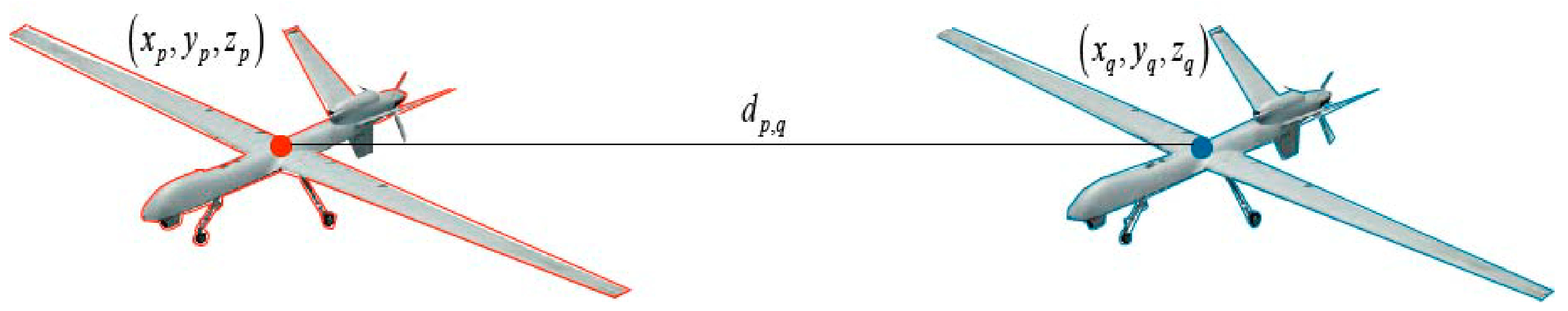
| Distance between the and UAVs | |
| Time when the UAV arrives at the task point | |
| Left and right time windows of the task point | |
| Task volume of the task point | |
| Maximum task volume that the UAV can complete |
| Zone Number | Center of the Bottom Circle | Radius |
|---|---|---|
| Cylinder no-fly zone 1 | (250,370) | 40 |
| Cylinder no-fly zone 2 | (140,250) | 35 |
| Point Number | X-Coordinate | Y-Coordinate | Demand | Left Time Window | Right Time Window | Service Time |
|---|---|---|---|---|---|---|
| Distribution Center | 25 | 30 | / | 0 | 1260 | / |
| 1 | 50 | 50 | 40 | 480 | 945 | 20 |
| 2 | 380 | 50 | 10 | 456 | 900 | 20 |
| 3 | 50 | 450 | 40 | 48 | 225 | 20 |
| 4 | 450 | 220 | 10 | 432 | 855 | 20 |
| 5 | 250 | 250 | 20 | 16 | 90 | 20 |
| 6 | 100 | 100 | 10 | 384 | 780 | 20 |
| 7 | 120 | 110 | 40 | 128 | 300 | 20 |
| 8 | 130 | 120 | 30 | 176 | 405 | 20 |
| 9 | 300 | 100 | 10 | 368 | 750 | 20 |
| 10 | 300 | 120 | 5 | 240 | 495 | 20 |
| 11 | 400 | 350 | 17 | 312 | 660 | 20 |
| 12 | 420 | 360 | 3 | 392 | 825 | 20 |
| 13 | 150 | 380 | 16 | 72 | 225 | 20 |
| 14 | 80 | 420 | 23 | 344 | 753 | 20 |
| 15 | 480 | 80 | 31 | 272 | 600 | 20 |
| Category | Function Name | Expression | Theoretical Optimal Value |
|---|---|---|---|
| Unimodal Test Function | Sphere Function | 0 | |
| Quartic Function | 0 | ||
| Multimodal Test Function | Ackley’s Function | 0 | |
| Fixed-dimension Multimodal Test Function | Branin Function | 0.39788735 | |
| Kowalik Function | 0.0003075 |
| Test Function | Data Type | ACO | PSO | WOA | IWOA |
|---|---|---|---|---|---|
| Mean Value | 100,222.22 | 12,324.9345 | 0.6090 | 0.00077 | |
| Best Value | 100,222.22 | 3874.1177 | 0.05230 | 1.64983 × 10⁻⁵ | |
| Mean Value | 5,605,894,559 | 202,601,216.1 | 33.5324 | 0.119037 | |
| Best Value | 4,579,640,494 | 37,290,487.49 | 1.2149 | 0.01651 | |
| Mean Value | 21.7181 | 19.9999 | 20.4272 | 20.27560 | |
| Best Value | 21.7180 | 19.9999 | 20.1486 | 20.05561 | |
| Mean Value | 15.9554 | 1.1616 | 0.6112 | 0.655569 | |
| Best Value | 14.5972 | 0.3986 | 0.3979 | 0.3979 | |
| Mean Value | 0.1170 | 0.0063 | 0.0024 | 0.0013 | |
| Best Value | 0.0156 | 0.0011 | 0.0010 | 0.0009 |
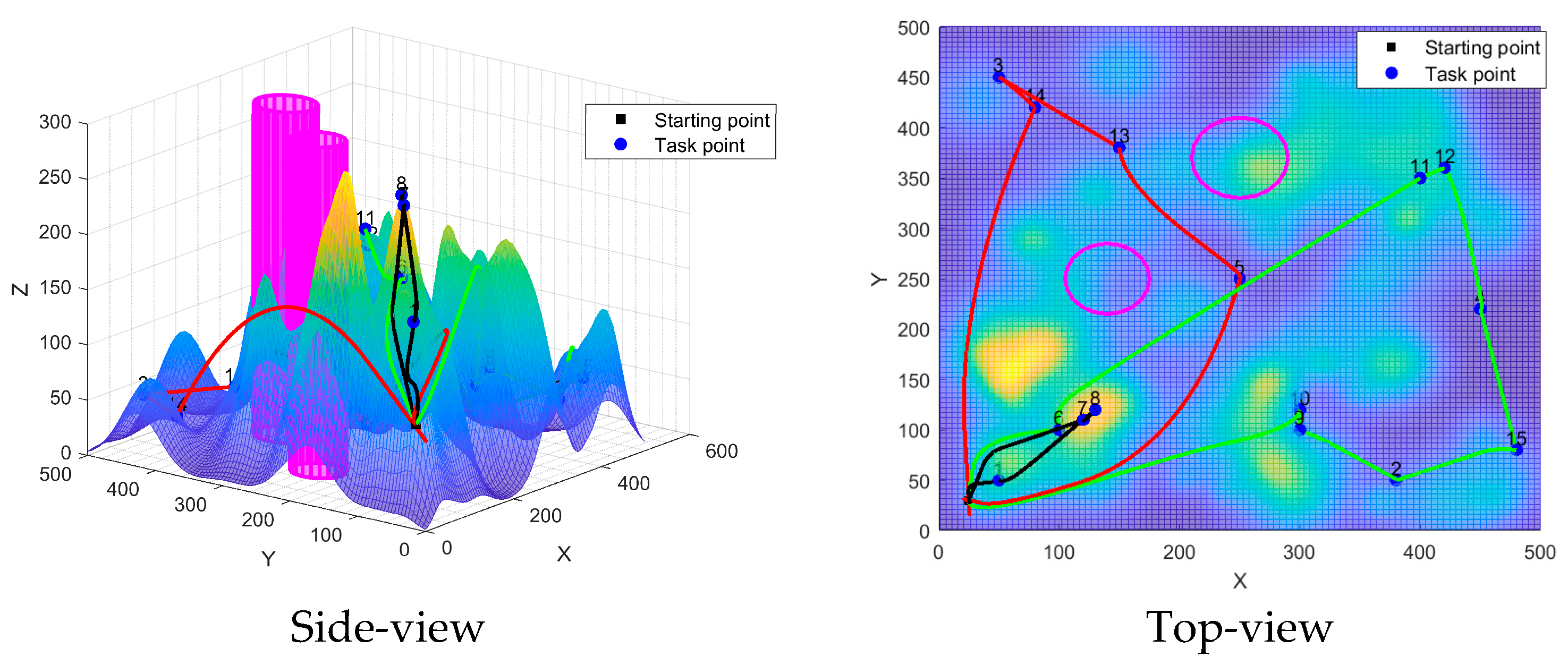
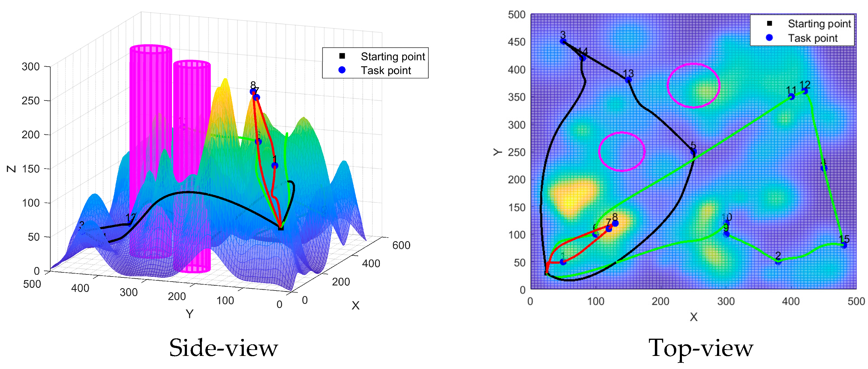
| Algorithm | Drone | Task Points | Flight Distance | Task Volume | Total Flight Distance | Total Fitness |
|---|---|---|---|---|---|---|
| IALNS-IWOA | 1 | 0-8-7-1-0 | 461.30792 | 110 | 2961.5315 | 4019.38625 |
| 2 | 0-5-13-3-14-0 | 1054.25558 | 99 | |||
| 3 | 0-10-9-2-15-4-12-11-6-0 | 1445.96800 | 96 | |||
| IALNS-WOA | 1 | 0-13-3-14-10-9-0 | 1227.17871 | 94 | 3194.65192 | 4338.738 |
| 2 | 0-7-8-1-0 | 462.48449 | 110 | |||
| 3 | 0-5-11-12-4-15-2-6-0 | 1504.98872 | 101 | |||
| IALNS-PSO | 1 | 0-7-8-1-0 | 462.48449 | 110 | 3063.74593 | 4147.02121 |
| 2 | 0-5-13-3-14-0 | 1054.25558 | 99 | |||
| 3 | 0-9-10-2-15-4-12-11-6-0 | 1547.00586 | 96 | |||
| IALNS-ACO | 1 | 0-7-1-6-0 | 566.87832 | 90 | 3543.66885 | 6603.29729 |
| 2 | 0-3-13-14-8-0 | 1238.45150 | 109 | |||
| 3 | 0-5-10-2-9-15-4-12-11-0 | 1738.33903 | 106 |
| Algorithm | Drone | Task Points | Flight Distance | Task Volume | Total Flight Distance | Total Fitness | |
|---|---|---|---|---|---|---|---|
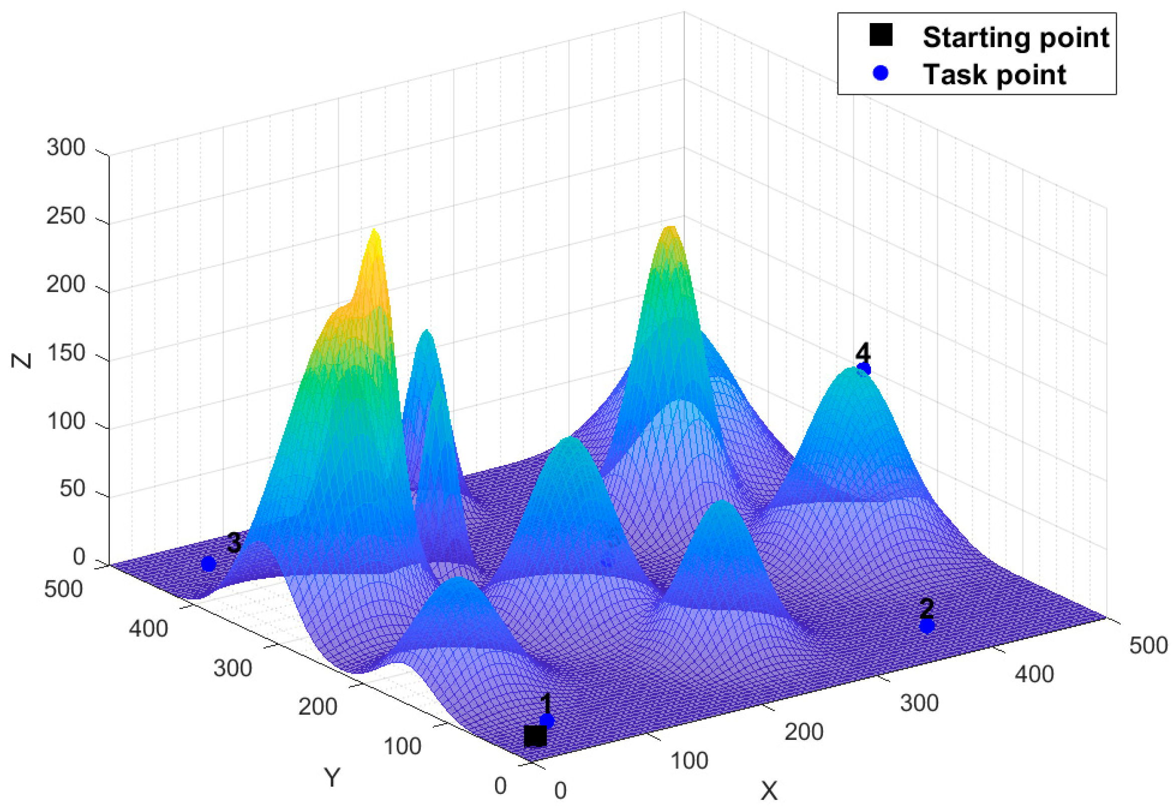
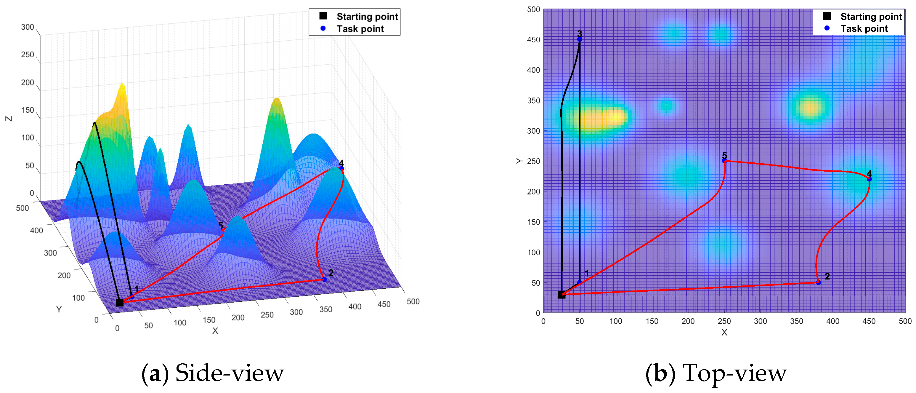
| IALNS-IWOA | 1 | 0-3-1-0 | 852.76203 | 80 | 1973.14747 | 998.83682 | |
| 2 | 0-5-4-2-0 | 1120.38544 | 40 | ||||
| Point Number | X-Coordinate | Y-Coordinate | Demand | Left Time Window | Right Time Window | Service Time |
|---|---|---|---|---|---|---|
| 16 | 280 | 180 | 12 | 256 | 540 | 20 |
| 17 | 350 | 260 | 25 | 144 | 330 | 20 |
| 18 | 190 | 300 | 28 | 320 | 660 | 20 |
| 19 | 410 | 140 | 14 | 192 | 420 | 20 |
| 20 | 200 | 230 | 9 | 400 | 810 | 20 |
| Center of the Bottom Circle | Radius |
|---|---|
| (400,100) | 20 |
| Algorithm | Drone | Task Points | Flight Distance | Task Volume | Total Flight Distance | Total Fitness |
|---|---|---|---|---|---|---|
| IALNS-IWOA | 1 | 0-8-7-6-0 | 372.88136 | 80 | 4130.72609 | 1953.13468 |
| 2 | 0-5-19-17-11-12-16-10-0 | 1366.03646 | 96 | |||
| 3 | 0-13-3-14-18-0 | 1085.99370 | 107 | |||
| 4 | 0-9-2-15-4-20-1-0 | 1305.81457 | 110 |
Disclaimer/Publisher’s Note: The statements, opinions and data contained in all publications are solely those of the individual author(s) and contributor(s) and not of MDPI and/or the editor(s). MDPI and/or the editor(s) disclaim responsibility for any injury to people or property resulting from any ideas, methods, instructions or products referred to in the content. |
© 2025 by the authors. Licensee MDPI, Basel, Switzerland. This article is an open access article distributed under the terms and conditions of the Creative Commons Attribution (CC BY) license (https://creativecommons.org/licenses/by/4.0/).
Share and Cite
Yang, Y.; Fu, Y.; Xin, R.; Feng, W.; Xu, K. Multi-UAV Trajectory Planning Based on a Two-Layer Algorithm Under Four-Dimensional Constraints. Drones 2025, 9, 471. https://doi.org/10.3390/drones9070471
Yang Y, Fu Y, Xin R, Feng W, Xu K. Multi-UAV Trajectory Planning Based on a Two-Layer Algorithm Under Four-Dimensional Constraints. Drones. 2025; 9(7):471. https://doi.org/10.3390/drones9070471
Chicago/Turabian StyleYang, Yong, Yujie Fu, Runpeng Xin, Weiqi Feng, and Kaijun Xu. 2025. "Multi-UAV Trajectory Planning Based on a Two-Layer Algorithm Under Four-Dimensional Constraints" Drones 9, no. 7: 471. https://doi.org/10.3390/drones9070471
APA StyleYang, Y., Fu, Y., Xin, R., Feng, W., & Xu, K. (2025). Multi-UAV Trajectory Planning Based on a Two-Layer Algorithm Under Four-Dimensional Constraints. Drones, 9(7), 471. https://doi.org/10.3390/drones9070471