A Novel Neural Network-Based Adaptive Formation Control for Cooperative Transportation of an Underwater Payload Using a Fleet of UUVs

Abstract

This article studies the cooperative underwater payload transportation problem for multiple unmanned underwater vehicles (UUVs) operating in a constrained workspace with both static and dynamic obstacles. A novel cooperative formation control algorithm has been presented in this paper for the transportation of a large payload in underwater scenarios. More precisely, by using the advantages of multi-UUV formation cooperation, based on rigidity graph theory and backstepping technology, the distance between each UUV, as well as the UUV and the transport payload, is controlled to form a three-dimensional rigid structure so that the load remains balanced and stable, to coordinate the transport of objects within the feasible area of the workspace. Moreover, a neural network (NN) is utilized to maintain system stability despite unknown nonlinearities and disturbances in the system dynamics. In addition, based on the interfered fluid flow algorithm, a collision-free motion trajectory was planned for formation systems. The control scheme also performs real-time formation reconfiguration according to the size and position of obstacles in space, thereby enhancing the flexibility of cooperative handling. The uniform ultimate boundedness of the formation distance errors is comprehensively demonstrated by utilizing the Lyapunov stability theory. Finally, the simulation results show that the UUVs can quickly form and maintain the desired formation, transport the payload along the planned trajectory to shuttle in multi-obstacle environments, verify the feasibility of the method proposed in this paper, and achieve the purpose of the collaborative transportation of large underwater payload by multiple UUVs and their targeted delivery.

1. Introduction

Over the past few years, the employment of unmanned underwater vehicles (UUVs) in numerous applications, including underwater exploration, oceanic surveillance, and marine resource utilization, has shown a significant growth trend [1]. Compared to a single UUV, a multi-UUV formation can achieve more complex and large-scale tasks through collaborative work, such as monitoring large areas of the marine environment, searching for and tracking underwater targets, and exploring marine resources [2]. Formation control technology, as the core of multi-UUV cooperative operations, ensures that each vehicle can move according to the predetermined formation and effectively coordinate the relationship between position and speed, which is crucial for improving the overall efficiency of the multi-UUV system [3].

Even though a significant number of results have been achieved in multi-UUV formation cooperation [4,5,6,7], they rarely focus on particular underwater applications. Apart from the existing and intensively investigated manipulation scenarios described in [8,9,10], the cooperative transportation of underwater payloads represents a formidable task in UUV operations, and this area remains uncharted mainly territory [8]. In the complex and varied multi-obstacle underwater environment affected by ocean currents, coordinating multiple UUVs to form a stable formation around the payload and transport it to the desired location is a challenge. Another significant challenge is planning a movement path for the formation and dynamically generating flexible, reconfigurable transport formations that respond to the a changing environment.

Object transportation is a common practice in various practical applications [11], but it is challenging to use the UUV to carry out object transportation in the underwater environment where space size is limited or there is danger. Because objects may have arbitrary shapes, uneven weight distribution, or discontinuous surfaces, a simple UUV structure may not be sufficient to achieve stable transport. Therefore, the task of using UUVs to transport underwater objects while meeting the complex trajectory planning requirements and ultimately reaching the target point within a limited environment is an urgent and challenging problem that has not been widely explored. Assuming that the weight of the object exceeds the carrying capacity of a single UUV, compared with the design characteristics of the heavy UUV with fixed size and low flexibility, the multi-UUV cooperative transportation system can not only adjust the formation and size of the formation according to the shape of the object to be transported to adapt to the porters, realize the diversification of handling types, but also maneuver according to the planned trajectory, avoid obstacles to improve work efficiency [12].

In [13], the authors present the results of cooperative transportation of a lengthy object using two underwater vehicle manipulator systems (UVMSs), relying on a restricted amount of information exchange among the agents. In [14], the issue of cooperative object transportation for multiple UVMSs within a workspace with constraints and static obstacles has been investigated. Here, the leader-follower strategy is considered, and two UVMSs form a formation heading toward the target configuration while evading collisions with the obstacles. This system was enhanced in [15], where a nonlinear model predictive control strategy was proposed to overcome significant constraints and limitations. In [16], the authors introduce a hierarchical method to derive the equations of motion using the Modular Modelling Methodology (MMM), thereby addressing the problem of transporting an object with two Intervention-Autonomous Underwater Vehicles (I-AUVs) along a predefined path. In [17], a multi-layer control method and a potential field approach based control strategy have been developed. This strategy is designed to handle the coordination of the swarm simultaneously, the guidance and navigation of the I-AUVs, and the manipulation task, taking into account the presence of obstacles. In [18], a path-following algorithm is designed to compute the desired velocities for the I-AUV end-effectors to transport a long pipe by multiple I-AUVs. Moreover, a strategy for coordinating the transport of underwater objects using multiple biomimetic robotic fish is proposed in [19]. In this method, the fuzzy logic approach is employed to control the transportation orientation, while the limit cycle approach is utilized to regulate the fish’s posture and ensure collision avoidance. Similarly, the work [20] also investigated the cooperative transport of an object by multiple biomimetic robotic fish, where a situated action selection approach is designed to realize the cooperative transportation task. However, all the aforementioned works consider the collaborative object transportation problem based on underwater vehicle manipulator systems, where the payload is transported by gripping with a robotic arm. On the other hand, few works consider the issue of underwater cable transportation systems.

In this study, we will explore the theories of formation control and motion planning for transportation and delivery tasks carried out by a fleet of UUVs using the cable payload method, as illustrated in Figure 1. Our research takes inspiration from the formation planning challenges faced by tethered multirotor UAVs in cooperative transportation scenarios. Compared to transportation methods involving UVMSs, as detailed in [14], the suspended payload approach offers several advantages. It significantly reduces the mass and inertia of the system, allowing for a more favorable dynamic response, as documented in [21]. This method also leads to lower energy consumption and reduced mechanical complexity. However, it is essential to note that the payload introduces an additional degree of freedom for the UUVs, directly affecting their dynamic behavior and often resulting in swinging motions during navigation missions. In this work, we consider cable tension, influenced by multiple UUVs, as an external disturbance. Consequently, our control objective is to maintain an appropriate formation among the UUVs, even in the presence of these tension disturbances. Therefore, the primary aim of this paper is to ensure the safe transportation of the payload with minimal oscillation while maintaining the desired formation configuration and the stability of the UUVs, even when subjected to external perturbations.

The tension forces in the cables, generated by the weight of the payload, significantly affect the dynamics and stability of the UUVs. This impact is significant since these tension forces are not directly measurable. Traditional formation control methods [22,23,24,25] for UUVs often depend on predefined models and fixed control laws. However, the complexity and dynamic nature of the underwater environment, including ocean currents, varying water densities, and unforeseen obstacles, make it challenging for these methods to perform optimally when it comes to underwater collaborative transportation of a payload. One practical solution is to incorporate a neural network (NN) into the control system. This approach can help mitigate parametric uncertainties and various disturbances, both external and internal. NNs have demonstrated considerable potential in managing complex and uncertain systems due to their ability to learn from data and adapt to changing conditions [26,27].

Although previous studies have proposed various control algorithms to address cooperative transportation control issues, certain limitations persist. Specifically, these algorithms rarely consider formation motion planning and obstacle avoidance. In this work, in addition to maintaining the stability of the cooperative transport formation, we also designed a multi-UUV formation motion planning method to avoid collisions with underwater obstacles. Concerning the motion planning approaches, based on our most comprehensive literature review, the interfering fluid dynamical system (IFDS) method, which was initially introduced by Wang et al. in reference [28], seems to exhibit the most excellent practicality. This is achieved through global optimization, low computational cost, real-time implementation, smooth motion trajectories, the ability to handle complex 3-D environments, and dynamic obstacle avoidance capabilities [29,30,31,32]. In this work, we use the interfered fluid flow (IFF) algorithm to plan the formation motion trajectory, ensuring safety by realizing collision avoidance behavior when obstacles approach. Regarding the second challenge, adaptive control has been introduced to cope with system uncertainties [33], where the control approach based on NN can take it a step further to deal with the uncertainties inherent in nonlinear systems [34].

Therefore, the primary objective of this paper is to develop an innovative distributed control algorithm that addresses the issues above and enhances the performance of cooperative payload transportation and delivery tasks carried out by UUVs. Hence, compared with the current research, the main contributions of this study can be summarized as follows

• As far as we know, this study is the first to study cable-based collaborative underwater load transport. We fully consider the influence of ocean currents on collaborative transport and propose a formation controller based on adaptive control and neural networks. The results demonstrate that the control system is robust against uncertain system parameters, and the adaptive scheme can asymptotically obtain the ideal shape.
• Unlike the paper [34], where their controllers are designed using second-order nonlinear systems, a novel nonlinear adaptive controller is developed for Euler-Lagrange model based UUV systems. We will demonstrate that this controller significantly enhances the system’s ability to withstand external disturbances, thereby boosting its robustness.
• This paper proposes a reconfigurable formation motion planning mechanism for the cooperative transport of underwater payloads with multiple UUVs. The mechanism is efficient in trajectory planning, offering a smooth, continuous path that effectively sidestepping the common pitfall of getting trapped in local optima. It can manage diverse obstacle avoidance scenarios while ensuring the initial formation remains intact.

The remainder of this paper is structured as follows. Section 2 presents some basic definitions, including the UUV model, graph theory, NN, the environment model, and control objective. The proposed formation motion planning scheme based on IFF is presented in Section 3. Section 4 presents the rigidity graph (RG) based formation control scheme for the cooperative transportation systems. The results of numerical simulations, which are used to demonstrate the performance of the proposed scheme, are reported in Section 5. Finally, Section 6 concludes and outlines some areas for further research.

2. Preliminaries

2.1. Nomenclature

A list of key symbols and notations used in the multi-UUV formation system is presented in

Table 1. The meaning of key symbol and nomenclature used in the heterogeneous multi-UAV-UGV system.

Symbol	Definition	Symbol	Definition
${\mathbb{R}}^n$	n-dimensional Euclidean space	${\beta }_i$	Alternative error variable
${\mathbb{R}}^{m\times n}$	$m\times n$ real matrix space	$\mathcal{W}$, ${\mathcal{W}}_d$, ${\mathcal{W}}_{total}$	Lyapunov function
$I_n$	n-dimensional identity matrix	$v_f$	Alternative error variable
$1_n$	1-column vector	$\tilde{v}$	Introduced velocity variable
$\mathcal{G}=(\mathcal{V},\mathcal{E},\mathcal{A})$	Undirected graph	$v_d$	Intended navigation speed of UUV
$\mathcal{V}=\{1,2,\dots ,n\}$	Set of vertices	$p_v$	Position of planned waypoint
$\mathcal{E}\subseteq \mathcal{V}\times \mathcal{V}$	Set of edges	$p_{obs}$	Position of obstacle
$\mathcal{A}=\left[a_{ij}\right]{\in }^{n\times n}$	The adjacency matrix	$p_g$	Position of goal
$\mathcal{F}$	Formation framework	$C_0$	The maneuvering velocity of the flow
${\mathcal{N}}_i$	Neighbor set of the UUV i	$\Gamma \left(p_v\right)$	Obstacle function
n	Number of UUVs	$v\left(p_v\right)$	Initial navigation speed of $p_v$
$M_i$	Inertia matrix	$H_k\left(p_v\right)$	Interfering modulation matrix of kth obstacle
$C_i$	Dentripetal/Coriolis terms matrix	$\overline{H}\left(p_v\right)$	Total interfering modulation matrix
$D_i$	Damping matrix	$\omega \left(p_v\right)$	Weighting coefficient of kth obstacle
$p_i={[x_i,y_i,z_i]}^T$	Position of UUV i	$n_k$	Radial normal vector of kth obstacle
${\theta }_i$, ${\phi }_i$	Heading angle of UUV i	$t_k$	Tangent vector of kth obstacle
$J(·)$	Conversion matrix	${\rho }_k$	Influence radius of the obstacle of kth obstacle
$v_i$	Linear velocity of UUV i	${\sigma }_k$	Tangential reaction coefficient of kth obstacle
${\tau }_i$	Control input of UUV i	K	Number of obstacles
$Y_i$	Regression matrix	$\overline{v}\left(p_v\right)$	Total disturbance flow velocity
${\varphi }_i$	Model parameter	$v_{obs}^k$	Velocity vector of kth dynamic obstacle
${\widehat{\varphi }}_i$	Parameter estimation of ${\varphi }_i$	$k_a$, $k_v$, $k_m$	Parameters of formation controller
${\tilde{\varphi }}_i$	Parameter estimation error	$W^T$, $V^T$	NN weights
${\tau }_w$	External disturbance	$\psi$	NN activation function
$R\left(p\right)$	Rigidity matrix	L	Hidden neurons
$d_{ij}\left(t\right)$	Desired distance between two UUV i and j	$diag\{·\}$	Diagonal matrix
${\tilde{p}}_{ij}$	Distance between two UUV i and j	$A^T$	Transposition of the matrix A
$e_{ij}$	Distance error	⊗	Kronecker product
$d_{safe}$	Safe distance	$∥·∥$	2-norm of a vector

.

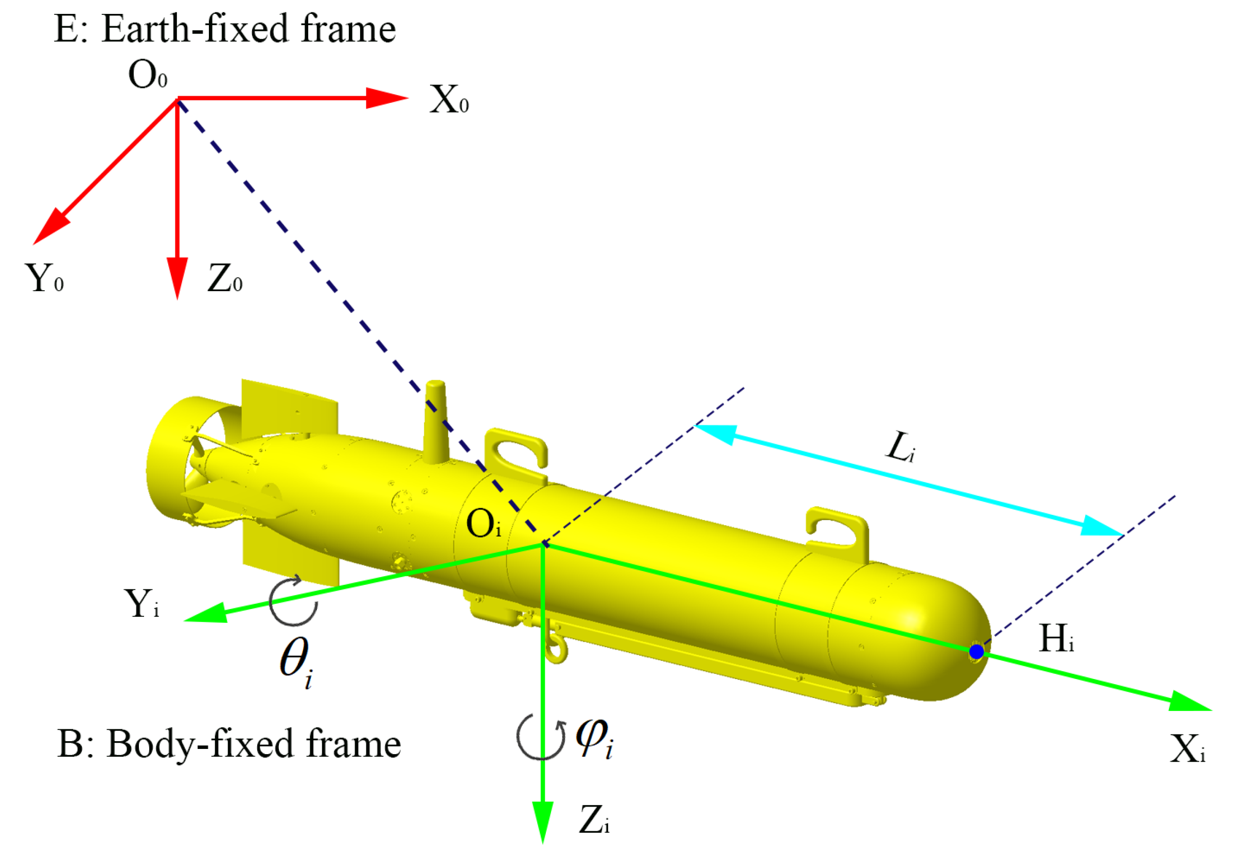
2.2. Modeling the UUV Kinematics

To facilitate the discussion of collaborative transportation formation control and motion planning of multi-UUV systems, the following assumptions are presented to elucidate the design of the controller.

Assumption 1. 

Each UUV is outfitted with a diverse array of reliable navigation sensors in the multi-UUV formation maneuvering system. These include sonar, an inertial navigation system, an ultra-short baseline, an underwater vision camera, an altimeter, an Ultrasonic sensor, and underwater Lidar. Integrating these combined navigation sensors empowers each UUV to achieve accurate navigation and effective perception of underwater obstacles.

Assumption 2. 

For the multi-UUV formation cooperative transportation system, based on Assumption 1, each UUV can measure the distance to adjacent UUVs and the transported payload in real time.

We consider a formation transportation system consisting of n transport UUVs in a 3-D ocean environment. Figure 2 shows the ith UUV, where the earth-fixed frame is denoted by $\left\{E\right\}=\{X_0,Y_0,Z_0\}$ and the body-fixed frame by $\left\{B\right\}=\{X_i,Y_i,Z_i\}$. Then, the kinematic and dynamic model of each UUV can be described by [33,35]

$${\dot{p}}_{ci}=S({\theta }_i,{\phi }_i){\eta }_i$$

(1)

$${\overline{M}}_i{\dot{\eta }}_i+{\overline{D}}_i{\eta }_i={\overline{\tau }}_i+{\overline{\tau }}_{wi}$$

(2)

in which, $p_{ci}={[x_{ci},y_{ci},z_{ci},{\theta }_i,{\phi }_i]}^T$ is the position of the mass point $(x_{ci},y_{ci},z_{ci})$ and the heading angles $({\theta }_i,{\phi }_i)$ of ith UUV relative to the frame $\left\{E\right\}$.The vector ${\eta }_i={[v_i,w_{\theta i},w_{\phi i}]}^T\in {\mathbb{R}}^3$, where $v_i$ denotes the linear velocity of ith transport UUV in the frame $\left\{E\right\}$, $w_{\theta i}$ and $w_{\phi i}$ represent the angular velocities about the z-axis and x-axis, respectively. $S({\theta }_i,{\phi }_i)$ is the transformation matrix and denoted as

$$\begin{array}{c}\hfill S({\theta }_i,{\phi }_i)=\left[\begin{array}{ccc}c{\theta }_{i}c{\phi }_i& 0& 0\\ c{\theta }_{i}s{\phi }_i& 0& 0\\ s{\theta }_i& 0& 0\\ 0& 1& 0\\ 0& 0& 1\end{array}\right]\end{array}$$

(3)

in which, $c{\theta }_i\stackrel{\Delta }{=}cos{\theta }_i$, $c{\phi }_i\stackrel{\Delta }{=}cos{\phi }_i$, $s{\theta }_i\stackrel{\Delta }{=}sin{\theta }_i$ and $s{\phi }_i\stackrel{\Delta }{=}sin{\phi }_i$, respectively. In (1b), ${\overline{M}}_i=\mathrm{diag}\{m_i,I_{i1},I_{i2}\}$ represents the inertia matrix, in which $m_i$ and $I_{i1}$, $I_{i2}$ are the ith UUV’s mass and moment of inertia about the axes, respectively. ${\overline{D}}_i\in {\mathbb{R}}^{3\times 3}$ denotes the constant damping matrix, ${\overline{\tau }}_i\in {\mathbb{R}}^3$ is the force/torque-level control input of the ith UUV, and ${\overline{\tau }}_{wi}\in {\mathbb{R}}^3$ is the bounded disturbing force of the unknown marine disturbances and satisfy $∥{\overline{\tau }}_{wi}∥\le {\tau }_{wM}$. From (1), one can note that the motion constraint space (${\eta }_i\in {\mathbb{R}}^3$) has a lower dimensionality compared to the system state space ($p_{ci}\in {\mathbb{R}}^5$). Therefore, to deal with the nonholonomic constraints and dynamic model constraints problem of UUVs, we follow the approach adopted in [33,36] and define the subsequent hand position $p_i={[x_i,y_i,z_i]}^T\in {\mathbb{R}}^3$ for the ith UUV as shown in Figure 2.

$$\begin{array}{c}\hfill p_i=\left[\begin{array}{c}{x}_i\\ y_i\\ z_i\end{array}\right]=\left[\begin{array}{c}{x}_{ci}\\ y_{ci}\\ z_{ci}\end{array}\right]+L_i\left[\begin{array}{c}c{\theta }_{i}c{\phi }_i\\ c{\theta }_{i}s{\phi }_i\\ s{\theta }_i\end{array}\right]\end{array}$$

(4)

with $L_i$ being the distance from the mass center of the ith UUV to defined point $H_i$, as shown in Figure 2. Then, by taking the derivative of $p_i$, we obtain

$$\begin{array}{c}\hfill {\dot{p}}_i=\left[\begin{array}{ccc}c{\theta }_{i}c{\phi }_i& -L_{i}c{\theta }_{i}s{\phi }_i& -L_{i}s{\theta }_{i}c{\phi }_i\\ c{\theta }_{i}s{\phi }_i& L_{i}c{\theta }_{i}c{\phi }_i& -L_{i}s{\theta }_{i}c{\phi }_i\\ s{\theta }_i& 0& L_{i}c{\theta }_i\end{array}\right]{\eta }_i\end{array}$$

(5)

Then, according to (1)–(4), we have

$$\begin{array}{c}\hfill {\eta }_i=J({\theta }_i,{\phi }_i){\dot{p}}_i\end{array}$$

(6)

where

$$\begin{array}{c}\hfill J({\theta }_i,{\phi }_i)=\left[\begin{array}{ccc}c{\theta }_{i}c{\phi }_i& c{\theta }_{i}c{\phi }_i& s{\theta }_i\\ -s{\phi }_i/L_{i}c{\theta }_i& c{\phi }_i/L_{i}c{\theta }_i& 0\\ -s{\theta }_{i}c{\phi }_i/L_i& -s{\theta }_{i}s{\phi }_i/L_i& c{\theta }_i/L_i\end{array}\right]\end{array}$$

Following the operation of taking the time derivative of (6), one have ${\dot{\eta }}_i=\dot{J}({\theta }_i,{\phi }_i){\dot{p}}_i+J({\theta }_i,{\phi }_i){\ddot{p}}_i$, and pre-multiplying the resulting equation by the matrix ${\overline{M}}_i$ in sequence, then substitute (2) to obtain

$$\begin{array}{c}\hfill {\overline{M}}_i\dot{J}({\theta }_i,{\phi }_i){\dot{p}}_i+{\overline{M}}_{i}J({\theta }_i,{\phi }_i){\ddot{p}}_i+{\overline{D}}_{i}J({\theta }_i,{\phi }_i){\dot{p}}_i={\overline{\tau }}_i+{\overline{\tau }}_{wi}\end{array}$$

(7)

Next, pre-multiply (7) by $J^T({\theta }_i,{\phi }_i)$, one obtain the following Euler-Lagrange-like dynamic model

$$\begin{array}{c}\hfill M_i\left(p_i\right){\ddot{p}}_i+C_i(p_i,{\dot{p}}_i){\dot{p}}_i+D_i\left(p_i\right){\dot{p}}_i={\tau }_i+{\tau }_{wi}\end{array}$$

(8)

where

$$\begin{array}{c}\hfill M_i\left(p_i\right)=J^T{\overline{M}}_{i}J,C_i(p_i,{\dot{p}}_i)=J^T{\overline{M}}_i\dot{J},D_i\left(p_i\right)=J^T{\overline{D}}_{i}J,{\tau }_i=J^T{\overline{\tau }}_i,{\tau }_{wi}=J^T{\overline{\tau }}_{wi}\end{array}$$

in which, $p_i\in {\mathbb{R}}^3$ stands for the generalized position of the ith UUV, $M_i\left(p_i\right)\in {\mathbb{R}}^{3\times 3}$ is the positive-definite inertia matrix, $C_i(p_i,{\dot{p}}_i)\in {\mathbb{R}}^{3\times 3}$ represents the Coriolis and centripetal matrix, $D_i\left(p_i\right)\in {\mathbb{R}}^{3\times 3}$ is the friction matrix, ${\tau }_i\in {\mathbb{R}}^3$ is the vector of control input, and ${\tau }_{wi}\in {\mathbb{R}}^3$ is the vector of bounded external disturbance.

For the Euler-Lagrange system (8), according to [33,37], there are three common important properties listed as follows, which play a crucial and beneficial role in the subsequent design and analysis.

Property 1. 

The mass matrix $M_i\left(p_i\right)$ a symmetric matrix that is both bounded and uniformly positive definite.

Property 2. 

Matrices $M_i\left(p_i\right)$ and $C_i\left(p_i,{\dot{p}}_i\right)$ satisfy ${\mu }^T(M_i\left(p_i\right)-2C_i(p_i,{\dot{p}}_i))\mu =0$ for any arbitrary vector $\mu \in {\mathbb{R}}^3$.

Property 3. 

Each system in (8) with parametric uncertainties can be rewritten as

$$\begin{array}{c}\hfill M_i\left(p_i\right){\dot{\mu }}_i+C_i(p_i,{\dot{p}}_i){\mu }_i+D_i\left(p_i\right){\dot{p}}_i=Y_i(p_i,{\dot{p}}_i,{\mu }_i,{\dot{\mu }}_i){\varphi }_i\end{array}$$

(9)

where $Y_i(p_i,{\dot{p}}_i,{\mu }_i,{\dot{\mu }}_i)$ is a known regression matrix, ${\varphi }_i\in {\mathbb{R}}^{12}$ represents a vector of unknown but constant dynamic parameters, which containing a series of physical associated with the ith UUV, and given as

$$\begin{array}{c}\hfill {\varphi }_i={\left[\begin{array}{c}{\left[\begin{array}{cccc}{m}_i& I_{i1}/L_i^2& I_{i1}/L_i^2& {\left({\overline{D}}_i\right)}_{11}\end{array}\right]}^T\\ {\left[\begin{array}{cccc}{\left({\overline{D}}_i\right)}_{12}/L_i& {\left({\overline{D}}_i\right)}_{13}/L_i& {\left({\overline{D}}_i\right)}_{21}/L_i& {\left({\overline{D}}_i\right)}_{22}/L_i^2\end{array}\right]}^T\\ {\left[\begin{array}{cccc}{\left({\overline{D}}_i\right)}_{23}/L_i^2& {\left({\overline{D}}_i\right)}_{31}/L_i& {\left({\overline{D}}_i\right)}_{32}/L_i^2& {\left({\overline{D}}_i\right)}_{33}/L_i^2\end{array}\right]}^T\end{array}\right]}^T\end{array}$$

2.3. Graph Theory

A communication topology of n formation transportation UUVs can be described by a weighted undirected graph $\mathcal{G}=(\mathcal{V},\mathcal{E},\mathcal{A})$ [38], where UUVs are represented by the vertices set $\mathcal{V}=\{1,2,\dots ,n\}$ of this graph, and the communication linkages between the UUVs are denoted by the edge set $\mathcal{E}\subseteq \mathcal{V}\times \mathcal{V}$. If the UUV i can receive information from the UUV j, then an edge is necessarily present between the vertices i and j, i.e., $(i,j)\in \mathcal{E}$, it is said UUV i and UUV j are adjacent. Using $\mathcal{A}=\left[a_{ij}\right]\in {\mathbb{R}}^{n\times n}$ stands for the adjacency matrix associated with the graph, where $a_{ij}$ indicates an undirected connection between UUVs i and j. If $(i,j)\in \mathcal{E}$, then $a_{ij}=1$; if not, $a_{ij}=0$. A vertex’s neighbors are the vertices from which it can obtain information, the set of neighbors of a vertex i is indicated by ${\mathcal{N}}_i\left(\mathcal{E}\right)=\left\{j\in \mathcal{V}\left|\right(i,j)\in \mathcal{E}\right\}$. $l\in \left\{1,2,\dots ,n(n-1)/2\right\}$ yields the number of edges l in the graph structure [38]. The edge function of $f_{\mathcal{G}}\left(p\right):{\mathbb{R}}^{3n}\to {\mathbb{R}}^l$ of $(\mathcal{G},p)$ is provided by

$$\begin{array}{c}\hfill f_{\mathcal{G}}\left(p\right)=(\dots ,{∥p_i-p_j∥}^2,\dots ),(i,j)\in \mathcal{E}\end{array}$$

(10)

in which, $∥·∥$ implies the Euclidean norm. From the edge function, one can define the rigidity matrix $R\left(p\right):{\mathbb{R}}^{3n}\to {\mathbb{R}}^{l\times 3n}$ of $(\mathcal{G},p)$ as follows

$$\begin{array}{c}\hfill R\left(p\right)={\displaystyle \frac{1}{2}}{\displaystyle \frac{\partial f_{\mathcal{G}}\left(p\right)}{\partial p}}\end{array}$$

(11)

It is well knowledge that if and only if $\left|\mathcal{E}\right|=3\left|\mathcal{V}\right|-6$, then a graph $\mathcal{G}=(\mathcal{V},\mathcal{E},\mathcal{A})$ is minimally rigid in 3-D space [38]. Thus, matrix $R\left(p\right)$ has full row rank. Given that matrix $R^T\left(p\right)$ has the full column rank and $rank\left[R\left(p\right)\right]=rank\left[R\left(p\right)R^T\left(p\right)\right]$, then $R\left(p\right)R^T\left(p\right)\in {\mathbb{R}}^{\left|\mathcal{E}\right|\times \left|\mathcal{E}\right|}$ is invertible [38].

Lemma 1 

([39]). Let $\mu \left(t\right)\in {\mathbb{R}}^3$, and $1_n$ be the $n\times 1$ vector of ones, then $R\left(p\right)(1_n\otimes \mu )=0$.

2.4. Neural Network

Because the motion of UUV and the movement of the payload are affected by ocean currents and waves, a two-layer NN is used to estimate external disturbance. This NN consists of an input layer with a inputs and a layer of randomly assigned constant weights $V^T$, and an output layer with b outputs and a layer of tunable weights $W^T$. Additionally, L hidden neurons are taken into consideration. The expression is

$$\begin{array}{c}\hfill {\widehat{\tau }}_w={\widehat{W}}^T\psi \left(V^T\chi \right)\end{array}$$

(12)

where $\chi ={[1,x_1^T\left(t\right),x_2^T\left(t\right),\dots ,x_a^T\left(t\right)]}^T$ is the input vector for NN, ${\widehat{W}}_i$ is the weight vector estimate, $\psi (·)$ is the activation function of NN in the hidden layers. In this paper, we choose the sigmoid (logistic) function, that is, $\psi \left(\chi \right)=1/(1+e^{-\chi })$, as the activation function. We make this selection due to its simplicity and the notable properties it possesses, such as a straightforward structure, which enables a quicker training process and facilitates convergence.

The function approximation property of NN holds significant importance and is commonly employed to approximate unknown continuous functions within the realm of control applications [40]. The universal approximation theorem posits that for any smooth function $f\left(\chi \right)$, there exists an NN with certain ideal weights W and V, along with a specific number of hidden layer nodes L such that

$$\begin{array}{c}\hfill f\left(\chi \right)=W^T\psi \left(V^T\chi \right)+\epsilon \end{array}$$

(13)

where $\epsilon$ represents the function approximation error of the NN. It has been demonstrated that when the weights V of the input layer are randomly chosen, the activation function $\psi \left(\overline{\chi }\right)=\psi \left(V^T\chi \right)$ creates a stochastic basis. Consequently, the approximation property is valid for all inputs within close proximity over a compact set $\Omega \in {\mathbb{R}}^k$ [40]. Moreover, the functional approximation error is bounded and adheres to the condition $∥\epsilon ∥\le {\epsilon }_N$, where ${\epsilon }_N$ is a known positive bound that is contingent upon the compact set $\Omega$ [40]. If the weights and biases V of the first layer are kept fixed, the NN exhibits a linear-in-the-parameter characteristic. In this case, the approximation property can be achieved by adjusting the weights and biases W of the second layer. For such an NN as [40], the approximation is valid, and the approximation error converges to zero at an order of $O(C/\sqrt{L})$, where the constant C independent of the number of hidden layer nodes L. It is assumed that the approximating weights W are bounded, satisfying the inequality ${∥W∥}_F\le W_m$, where ${∥·∥}_F$ represents the Frobenius norm. Given a matrix $A=\left[a_{ij}\right]$, the Frobenius norm is defined as follows

$$\begin{array}{c}\hfill {∥A∥}_F^2=\sum _{i,j}{a}_{ij}^2=tr\left(A^{T}A\right)\end{array}$$

(14)

with $tr\left(\right)$ being the trace operation that sums the diagonal elements of a square matrix.

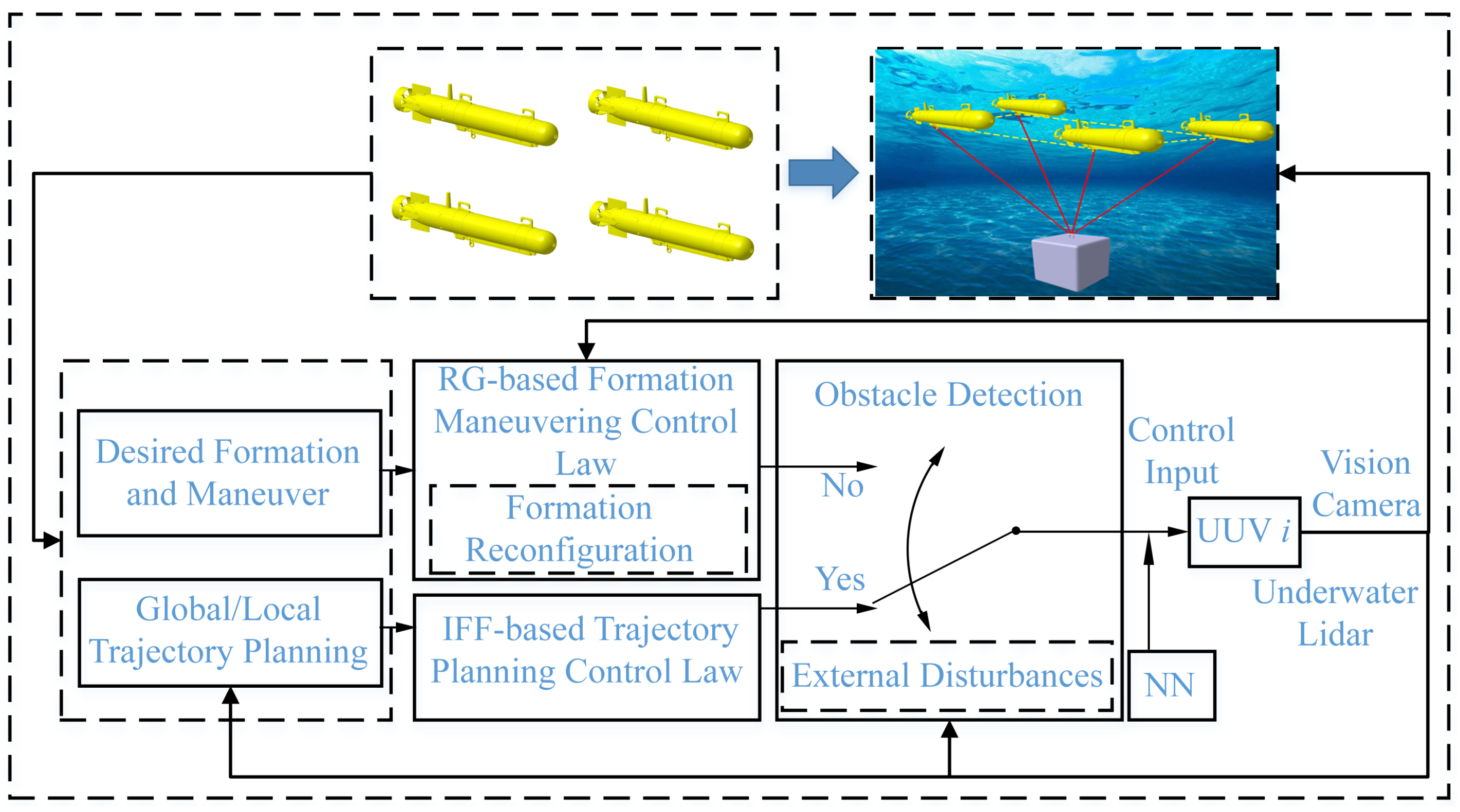
3. Motion Planning Design

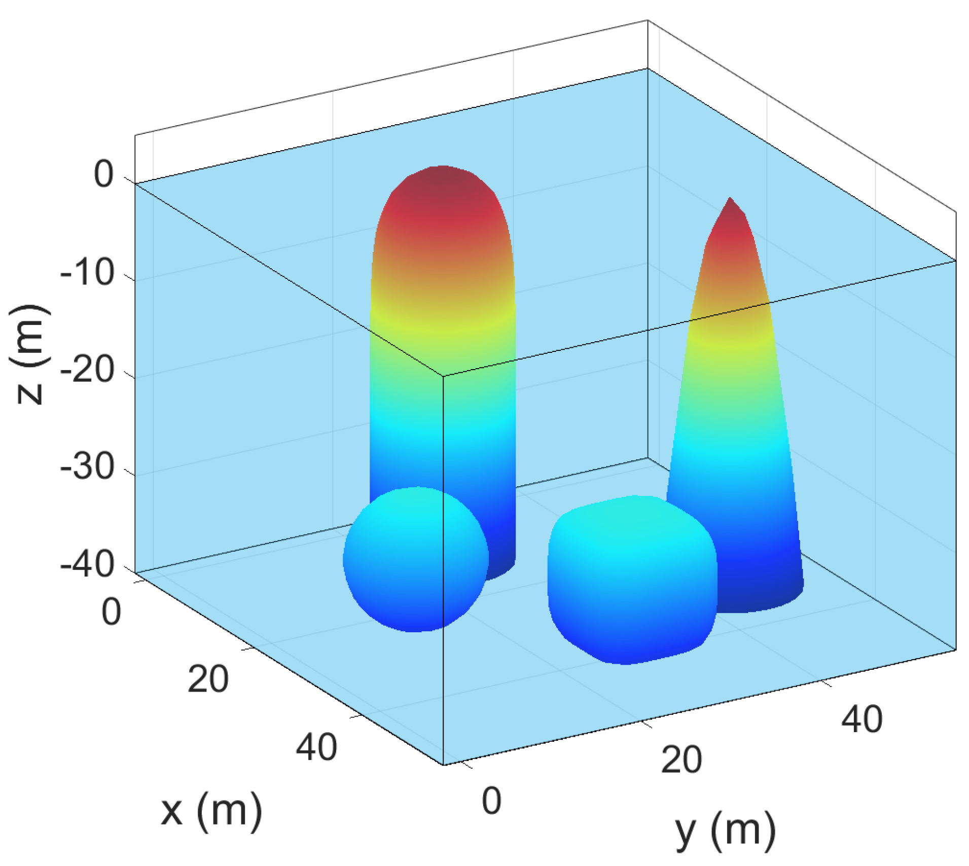
3.1. Modeling the Environment

In this paper, the formation of transport UUVs navigating in a 3-D multi-obstacle ocean environment to deliver a payload necessitates modeling obstacle space. The planned waypoint is labeled as a point $p_v=(x_v,y_v,z_v)$. In actual navigation and missions, the obstacles encountered are irregular. The standard convex polyhedrons can be used to enclose the barriers, which will reduce the complexity of the obstacle space. Assume the planning space contains K obstacles. After pretreatment, any obstacle can be represented by a standard convex polyhedron, such as a sphere, a cylinder, a cone, a cube, a parallelepiped, or an irregular body [28,30], as is shown in Figure 3. A unified standard model function $\Gamma$ is put forward to depict different kinds of irregular obstacles, and it can be expressed in the following manner

$$\begin{array}{c}\hfill \Gamma \left(p_v\right)={\left({\displaystyle \frac{x_v-x_{obs}}{a}}\right)}^{2\alpha }+{\left({\displaystyle \frac{y_v-y_{obs}}{b}}\right)}^{2\beta }+{\left({\displaystyle \frac{z_v-z_{obs}}{c}}\right)}^{2\gamma }\end{array}$$

(15)

where $p_{obs}=(x_{obs},y_{obs},z_{obs})$ represents the center of the obstacle, a, b, and c are the parameters that affect the size of the obstacle and are constants bigger than 0; $\alpha$, $\beta$, and $\gamma$ are the shape parameters that give various shapes. If $\Gamma \left(p_v\right)>1$, it means that $p_v$ is in the outside space of the obstacle; if $\Gamma \left(p_v\right)=1$, it implies that $p_v$ is on the surface of the obstacle; and if $\Gamma \left(p_v\right)<1$, it means that $p_v$ is in the inner space of the obstacle. If a, b, c and $\alpha$, $\beta$, $\gamma$ are constants, the obstacle described by function $\Gamma \left(p_v\right)=1$ can be approximated by the below convex polyhedron, subject to the following different conditions

$$\begin{array}{c}\hfill \mathrm{obstacle}=\left\{\begin{array}{c}\mathrm{sphere},\mathrm{if}\alpha =\beta =\gamma =1,\mathrm{and}a=b=c\\ \mathrm{cylinder},\mathrm{if}\alpha =\beta =1,\gamma >1,\mathrm{and}a=b\\ \mathrm{cone},\mathrm{if}\alpha =\beta =1,0<\gamma <1,\mathrm{and}a=b\\ \mathrm{parallelepiped},\mathrm{if}\alpha >1,\beta >,\gamma >1\end{array}\right.\end{array}$$

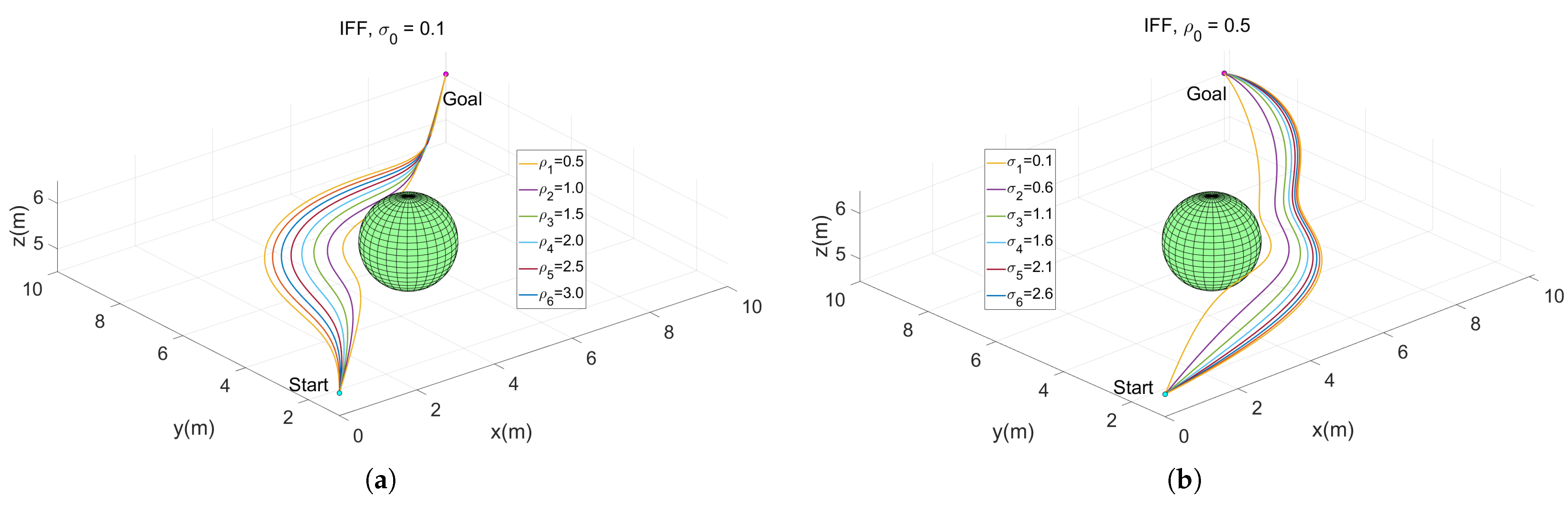
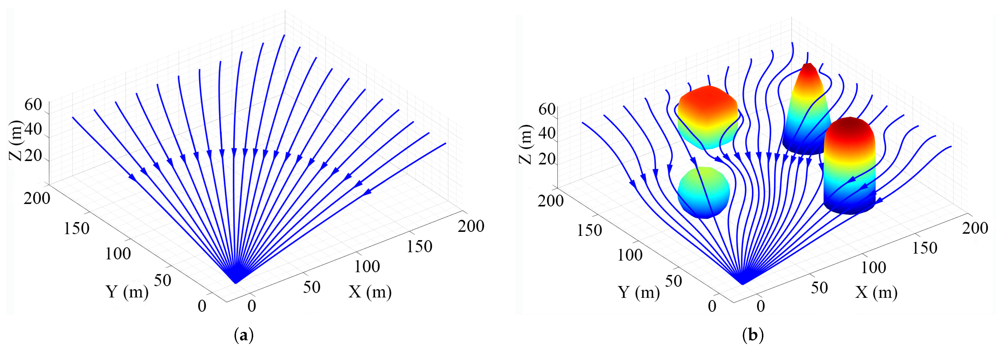
3.2. Formation Motion Planning

When there are no obstacles in the coordinated transport and delivery environment, the UUV will navigate directly from its current location to the delivery destination. Let’s denote $p_g=(x_g,y_g,z_g)$ as the goal delivery point, and the navigating velocity of the flow (or planned waypoints) is a constant, the distance between the current planned waypoint $p_v$ and the goal is $d(p_v,p_g)=\sqrt{{(x_v-x_g)}^2+{(y_v-y_g)}^2+{(z_v-z_g)}^2}$, then the initial expected flow speed in the 3-D space can be represented as [29]

$$\begin{array}{c}\hfill v\left(p_v\right)=-{\left({\displaystyle \frac{C_0(x_v-x_g)}{d(p_v,p_g)}}{\displaystyle \frac{C_0(y_v-y_g)}{d(p_v,p_g)}}{\displaystyle \frac{C_0(z_v-z_g)}{d(p_v,p_g)}}\right)}^T\end{array}$$

(16)

When the navigation space contains obstacles, the total interfering modulation matrix H can be used to characterize the influence of the impediments on the initial fluid speed:

$$\begin{array}{c}\hfill \overline{H}\left(p_v\right)=\sum _{k=1}^K{\omega }_k\left(p_v\right)H_k\left(p_v\right)\end{array}$$

(17)

in which, ${\omega }_k\left(p_v\right)$ denotes the kth obstacle’s coefficient of weight, and the value mostly depends on the distance between the currently planned waypoint and the obstacle’s surface. In general, the weight coefficient increases with decreasing distance., i.e., the greater the influence of obstacles on the original vector field. ${\omega }_k\left(p_v\right)$ may be defined in the form of

$$\begin{array}{c}\hfill {\omega }_k\left(p_v\right)=\left\{\begin{array}{c}1,K=1\\ {\displaystyle \prod _{i=1,i\ne k}^K}{\displaystyle \frac{({\Gamma }_i-1)}{({\Gamma }_i-1)+{\Gamma }_k-1}},K\ne 1\end{array}\right.\end{array}$$

(18)

From Formula (15), one can see that ${\Gamma }_i$, ${\Gamma }_k$ are obstacle equations. Due to ${\omega }_{sum}={\sum }_{k=1}^K{\omega }_k<1$, it should be normalized to ${\omega }_k={\omega }_k/{\omega }_{sum}$. $H_k$ is the kth obstacle’s interfering modulation matrix, and it is determined as follows:

$$\begin{array}{c}\hfill H_k\left(p_v\right)=I-{\displaystyle \frac{n_k{n}_k^T}{{\Gamma }_k^{1/{\rho }_k}{n}_k^T{n}_k}}+{\displaystyle \frac{t_k{n}_k^T}{{\Gamma }_k^{1/{\sigma }_k}∥t_k∥∥n_k∥}}\end{array}$$

(19)

in which, I is a third-order identity matrix, the second item is the repulsive matrix, where ${\rho }_k$ is the repulsive parameter and the third item is the tangential matrix, where ${\sigma }_k$ is the tangential parameter. $n_k$ describes the radial normal vector, and $t_k$ denotes the tangent vector. The shape of the streamline can be adjusted by changing $\rho$ and $\sigma$. The parameter $\rho$ defines the range in which the planned trajectory reacts to an obstacle. The bigger the response coefficient $\rho$, the earlier and greater the deflection from the original flow. On the other hand, the parameter $\sigma$ determines the degree of flexibility for lateral deviations of the planned trajectory. A greater $\sigma$ value makes the planned trajectory more adaptable to sideways changes. The effects of the tuning parameters $\rho$ and $\sigma$ is visually illustrated in Figure 4. It is possible to define $n_k$, $t_k$, ${\rho }_k$ and ${\sigma }_k$ in the following manners

$$n_k={\left[{\displaystyle \frac{\partial {\Gamma }_k}{\partial x}}{\displaystyle \frac{\partial {\Gamma }_k}{\partial y}}{\displaystyle \frac{\partial {\Gamma }_k}{\partial z}}\right]}^T$$

(20)

$$t_k={\left[{\displaystyle \frac{\partial {\Gamma }_k}{\partial y}}-{\displaystyle \frac{\partial {\Gamma }_k}{\partial x}}0\right]}^T$$

(21)

$${\rho }_k={\rho }_k^0{e}^{\left(1-{\displaystyle \frac{1}{d(p_v,p_g)d(p_v,p_{obs}^k)}}\right)}$$

(22)

$${\sigma }_k={\sigma }_k^0{e}^{\left(1-{\displaystyle \frac{1}{d(p_v,p_g)d(p_v,p_{obs}^k)}}\right)}$$

(23)

where, $d(p_v,p_g)$ denotes the distance separating the planned waypoint from the goal point, while $d(p_v,p_{obs}^k)$ indicates the distance between the planned waypoint and the kth obstacle’ surface. ${\rho }_k^0$ and ${\sigma }_k^0$ denote the initial reactivity parameters of kth obstacle.

Then the perturbation matrix correction is performed on the initial flow field $v\left(p_v\right)$, and the perturbed flow field is obtained

$$\begin{array}{c}\hfill \overline{v}\left(p_v\right)=\overline{H}\left(p_v\right)v\left(p_v\right)\end{array}$$

(24)

The initial stream from multiple starting points to a single target point $(0,0,0)$ is shown in Figure 5a. A sphere obstacle, a cylinder obstacle, a cone obstacle, and a cube obstacle are formed in Figure 5b, and their effects on the initial flow are shown. It is evident that the interfered flow lines may navigate obstacles with ease, accurately follow their contours, and eventually reach their destination. Finally, by integrating $\overline{v}\left(p_v\right)$ recursively, the next planned waypoint can be calculated

$$\begin{array}{c}\hfill {\left\{p_v\right\}}_{t+1}={\left\{p_v\right\}}_t+\overline{v}\left(p_v\right)·\Delta t\end{array}$$

(25)

where $\Delta t$ represents the iteration time step, all of the waypoints can be obtained by repeating the processes above. The route is smoother the smaller the calculation step size. Eventually, we’ll be able to get all of the intended waypoints, resulting in a modified streamline that is the planned path.

Next, let’s consider the situation where there are dynamic obstacles in the environment, then the perturbed fluid velocity $\overline{v}\left(p_v\right)$ can be obtained by modifying the initial flow field velocity $v\left(p_v\right)$

$$\begin{array}{c}\hfill \overline{v}\left(p_v\right)=\overline{M}\left(p_v\right)(v\left(p_v\right)-v_{obs}\left(p_v\right))+v_{obs}\left(p_v\right)\end{array}$$

(26)

where $v_{obs}\left(p_v\right)$ is the sum of the total velocity vector of the obstacles, and it is computed by the following formula

$$\begin{array}{c}\hfill v_{obs}\left(p_v\right)=\sum _{k=1}^K{w}_k{e}^{{\displaystyle \frac{-1}{{\lambda }_k}}({\Gamma }_k-1)}{v}_{obs}^k\left(p_v\right)\end{array}$$

(27)

in which, $v_{obs}^k\left(p_v\right)$ represents the velocity vector of the kth dynamic obstacle, ${\lambda }_k$ is a positive constant. Notably, the greater the value of ${\lambda }_k$, the sooner the streamline will initiate evasion of the dynamic obstacle. As a result, by appropriately choosing the value of ${\lambda }_k$, the streamline can successfully dodge the moving obstacle. The pseudo-code for the motion planning algorithm is shown in Algorithm 1.

Algorithm 1 Multi-AUU formation cooperative transportation motion planning based on IFF

Input:  1 formation start position ($p_v^0$), goal position ($p_g$), current velocity ($C_0$) Input:  2 obstacle numbers (K), obstacle position ($p_{obs}$), predicted obstacle speed ($v_{obs}$) Input:  3 obstacles type ($\alpha$, $\beta$, $\gamma$) and size (a, b, c) Output:  planned waypoint 1: while (mission uncompleted) do 2:    Update the motion information of planning waypoint 3:    Take the sink fluid as the initial fluid, and calculate the original fluid velocity by Equation (16) 4:    Update the information of dynamic obstacles or threats: model function ${\Gamma }_k\left(p_v\right)$, velocity $v_{obs}^k\left(p_v\right)$, $k\in 1,2,\dots ,K$ 5:    for each obstacle ${\Gamma }_k\left(p_v\right)$ do 6:      Compute the weighting coefficient by Equation (18) 7:      Compute the normal vector by Equation (20) 8:      Compute the tangent vector by Equation (21) 9:      Compute the modulation matrix by Equation (19) 10:   end for 11:   Calculate the overall modulation matrix by Equation (17) 12:   Calculate the overall velocity of dynamic obstacles by Equation (27) 13:   Calculate the disturbed fluid velocity by Equation (26) 14:   Obtain the next waypoint by Equation (25) 15:   Update the position ${\left\{p_v\right\}}_t={\left\{p_v\right\}}_{t+1}$ 16: end whilereturn 17: return Outputs

4. Formation Control Design

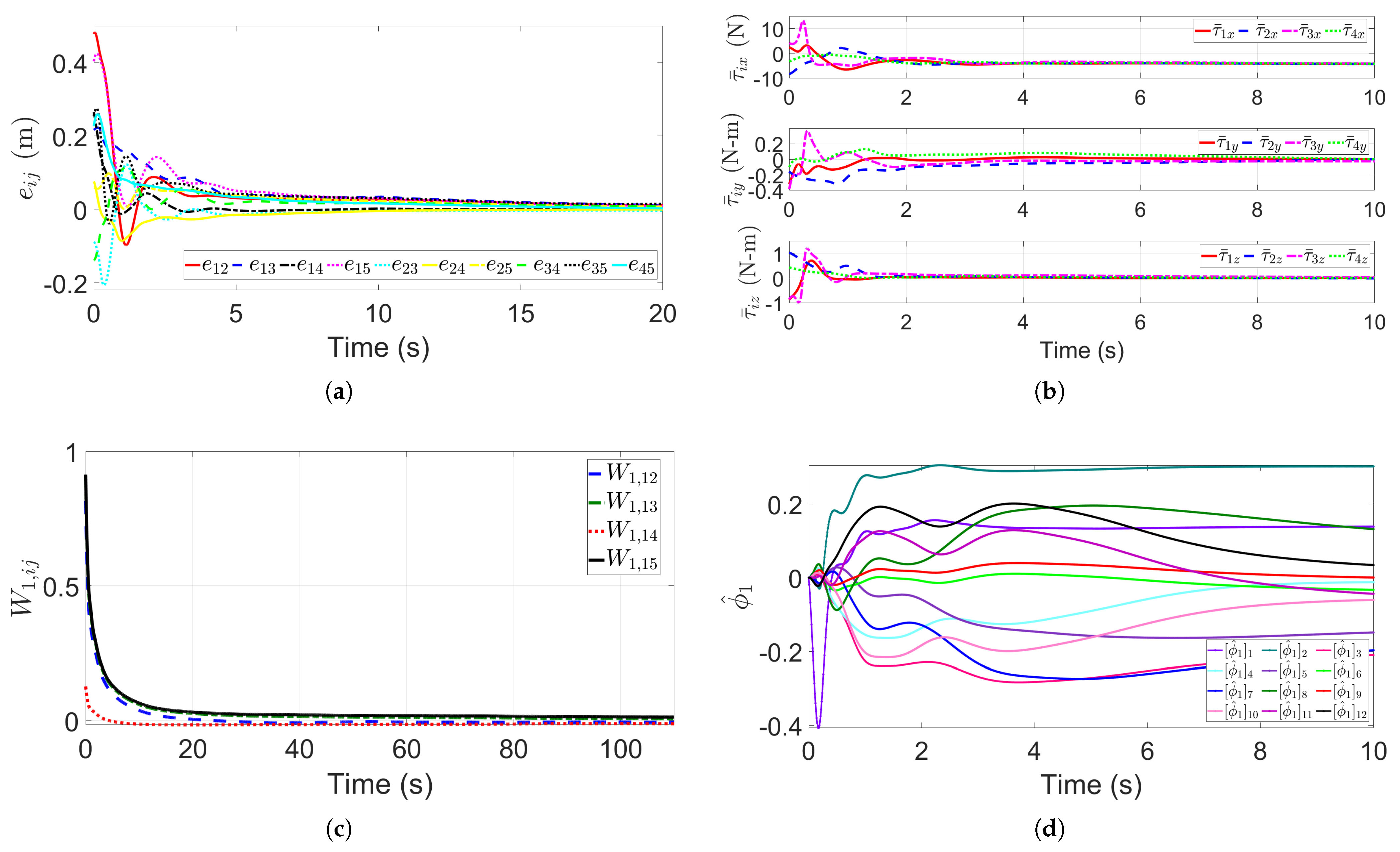
4.1. Formation Control Design

Let a rigid, time-variation framework ${\mathcal{F}}^{*}\left(t\right)=({\mathcal{G}}^{*},p^{*}\left(t\right))$ serve as the representation of the desired formation structure, in which, ${\mathcal{G}}^{*}=({\mathcal{V}}^{*},{\mathcal{E}}^{*})$, $dim\left({\mathcal{V}}^{*}\right)=n$, $dim\left({\mathcal{E}}^{*}\right)=l$ and $p^{*}=(p_1^{*},p_2^{*},\dots ,p_n^{*})\in {\mathbb{R}}^{3n}$. Then, the ideal separation between the UUVs as well as UUVs and payload node i and j can be denoted as

$$\begin{array}{c}\hfill d_{ij}\left(t\right)=∥p_i^{*}\left(t\right)-p_j^{*}\left(t\right)∥>d_{safe},i,j\in {\mathcal{V}}^{*}\end{array}$$

(28)

where $d_{safe}$ represents the minimum safety distance required to prevent a collision between the UUVs i and j in formation.

Thinking of the framework $\mathcal{F}\left(t\right)=({\mathcal{G}}^{*},p\left(t\right))$ as the real time-varying formation structure of UUVs, where $p=(p_1,p_2,\dots ,p_n)\in {\mathbb{R}}^{3n}$, at $t=0$, we assume that the distance between nodes in the current formation is different from the distance constraint between nodes in the desired formation structure, i.e., $∥p_i\left(0\right)-p_j\left(0\right)∥\ne d_{ij},i,j\in {\mathcal{V}}^{*}$.

The control goal of this article is to achieve time-varying formation reconfiguration and obstacle avoidance of multi-UUV systems in the 3-D obstacle environment. To achieve this, we consider the payload to be the leader and the transport UUVs to be followers. Our control process is broken down into the following steps: (a) Formation of UUVs is treated as a unit. When navigating in an obstacle environment, a feasible obstacle avoidance path is planned according to the detected obstacles. This planned path can be regarded as the known tracking point of the formation; (b) during maneuvering and avoiding obstacles, the payload tracks the intended path; and (c) the transportation UUVs keep the desired variable formation and follow the payload. We suppose that the payload knows the absolute velocity ${\dot{p}}_v$ and relative position $p_v-p_n$ of the planned waypoint and can share this vital information about formation control with the transport UUVs.

The first control goal is to design the obstacle avoidance path for formation UUVs, and we use the IFF method. Then we turn our attention to the second and third control objective, the issue of formation maintenance and formation reconfiguration. Therefore, the control goal is to design ${\tau }_i={\tau }_i(p_i,p_i-p_j,v_i,v_i-v_j,d_{ij},{\dot{d}}_{ij}),i=1,2,\dots ,n$ where $j\in {\mathcal{N}}_i\left({\mathcal{E}}^{*}\right)$ such that

$$\begin{array}{c}\hfill ∥p_i\left(t\right)-p_j\left(t\right)∥\to d_{ij}\left(t\right)\mathrm{as}t\to \infty ,(i,j)\in {\mathcal{E}}^{*}\end{array}$$

(29)

The secondary goal in the formation maneuvering problem is

$$\begin{array}{c}\hfill {\dot{p}}_i\left(t\right)-v_d\left(t\right)\to 0\mathrm{as}t\to \infty ,i=1,2,\dots ,n\end{array}$$

(30)

in which, $v_d\in {\mathbb{R}}^3$ denotes the intended navigation speed for the formation of UUVs and is a bounded and continuous function, and every UUV has knowledge of it.

Consider the formation of UUV systems that possess an Euler-Lagrange-like dynamic model given by (8). We can rewrite (8) as follows

$${\dot{p}}_i=v_i$$

(31)

$$M_i\left(p_i\right){\dot{v}}_i={\tau }_i-C_i(p_i,v_i)v_i-D_i\left(p_i\right)v_i+{\tau }_{wi}$$

(32)

where $v_i\in {\mathbb{R}}^3$ denotes the velocity of ith UUV’s $H_i$ point with respect to the earth-fixed frame $\left\{E\right\}$. Two nodes in the formation are in the following relative position

$$\begin{array}{c}\hfill {\tilde{p}}_{ij}=p_i-p_i,(i,j)\in {\mathcal{E}}^{*}\end{array}$$

(33)

The following formulas provide the distance error between any two nodes in the formation, along with the associated dynamics of this distance error

$$\begin{array}{c}\hfill e_{ij}=∥{\tilde{p}}_{ij}∥-d_{ij}\left(t\right),(i,j)\in {\mathcal{E}}^{*}\end{array}$$

(34)

$$\begin{array}{c}\hfill {\dot{e}}_{ij}={\displaystyle \frac{{\tilde{p}}_{ij}^T(v_i-v_j)}{e_{ij}+d_{ij}}}-{\dot{d}}_{ij}\end{array}$$

(35)

Defining a term ${\beta }_{ij}={∥{\tilde{p}}_{ij}∥}^2-d_{ij}^2=e_{ij}(e_{ij}+2d_{ij}),(i,j)\in {\mathcal{E}}^{*}$, then the Lyapunov function is described as follows for the first iteration of backstepping

$$\begin{array}{c}\hfill {\mathcal{W}}_{ij}={\displaystyle \frac{1}{4}}{\beta }_{ij}^2\end{array}$$

(36)

For all the edges, the following Lyapunov function is now introduced

$$\begin{array}{c}\hfill {\mathcal{W}}_{ij}\left(e\right)=\sum _{(i,j)\in {\mathcal{E}}^{*}}{\mathcal{W}}_{ij}\left(e_{ij}\right)\end{array}$$

(37)

in which, $e=(\dots ,e_{ij},\dots )\in {\mathbb{R}}^l$, and the following formula gives the time derivative of Formula (37)

$$\begin{array}{c}\hfill \dot{\mathcal{W}}=\sum _{(i,j)\in {\mathcal{E}}^{*}}{e}_{ij}(e_{ij}+2d_{ij})[{\tilde{p}}_{ij}^T(v_i-v_j)-d_{ij}{\dot{d}}_{ij}]={\beta }^T(R\left(p\right)v-d_v)\end{array}$$

(38)

where $v=(v_1,v_2,\dots ,v_n)\in {\mathbb{R}}^{3n}$, $\beta =(\dots ,{\beta }_{ij},\dots )\in {\mathbb{R}}^l$, $d_v=(\dots ,d_{ij}{\dot{d}}_{ij},\dots )\in {\mathbb{R}}^l,(i,j)\in {\mathcal{E}}^{*}$.

Now, following to the backstepping approach, let’s bring in an auxiliary variable

$$\begin{array}{c}\hfill \tilde{v}=v-v_f\end{array}$$

(39)

in which, $v_f\in {\mathbb{R}}^{3n}$ represents the fictitious hand velocity input.

Note that the multi-UUV formation control strategy is to be proposed under the premise of assuming that the variable ${\varphi }_i$ in (9) is unknown. Then, we bring in the parameter estimation error for the ith UUV, which is expressed as follows

$$\begin{array}{c}\hfill {\tilde{\varphi }}_i={\widehat{\varphi }}_i-{\varphi }_i\end{array}$$

(40)

Then, consider the Lyapunov function of the following form

$$\begin{array}{c}\hfill {\mathcal{W}}_d(e,\tilde{v})=\mathcal{W}\left(e\right)+{\displaystyle \frac{1}{2}}{\tilde{v}}^{T}M\left(p\right)\tilde{v}\end{array}$$

(41)

Its time derivative is given as

$$\begin{array}{c}\hfill {\dot{\mathcal{W}}}_d=\dot{\mathcal{W}}+{\displaystyle \frac{1}{2}}({\stackrel{\dot{˜}}{v}}^{T}M\left(p\right)\tilde{v}+{\tilde{v}}^T\dot{M}\left(p\right)\tilde{v}+{\tilde{v}}^{T}M\left(p\right)\dot{\tilde{v}})\end{array}$$

(42)

Since ${\stackrel{\dot{˜}}{v}}^{T}M\left(p\right)\tilde{v}={\tilde{v}}^{T}M\left(p\right)\stackrel{v}{\dot{˜}}$ and based on Property 2, one can rewrite (40) as

$$\begin{array}{cc}\hfill {\dot{\mathcal{W}}}_d& ={\beta }^T(R\left(p\right)(\tilde{v}+v_f)-d_v)+{\tilde{v}}^{T}M\left(p\right)\stackrel{\dot{˜}}{v}+{\displaystyle \frac{1}{2}}{\tilde{v}}^T\dot{M}\left(p\right)\tilde{v}\hfill \\ \hfill & ={\beta }^T(R\left(p\right)v_f-d_v)+{\beta }^{T}R\left(p\right)\tilde{v}+{\tilde{v}}^T[\tau +{\tau }_w-C(p,\dot{p})({\dot{v}}_f+\tilde{v})-D\left(p\right)\dot{p}\hfill \\ \hfill & -M\left(p\right){\dot{v}}_f]\hfill \\ \hfill & ={\beta }^T(R\left(p\right)v_f-d_v)+{\tilde{v}}^T({\displaystyle \frac{1}{2}}\dot{M}\left(p\right)-C(p,\dot{p}))\tilde{v}+{\tilde{v}}^T[\tau +{\tau }_w-C(p,\dot{p})v_f\hfill \\ \hfill & -D\left(p\right)\dot{p}-M\left(p\right){\dot{v}}_f+R^T\left(p\right)\beta ]\hfill \\ \hfill & ={\beta }^T(R\left(p\right)v_f-d_v)+{\tilde{v}}^T[\tau +{\tau }_w-(M\left(p\right){\dot{v}}_f+C(p,\dot{p})v_f+D\left(p\right)\dot{p})+R^T\left(p\right)\beta ]\hfill \\ \hfill & ={\beta }^T(R\left(p\right)v_f-d_v)+{\tilde{v}}^T[\tau +{\tau }_w-Y(p,\dot{p},v_f,{\dot{v}}_f)\varphi +R^T\left(p\right)\beta ]\hfill \end{array}$$

(43)

where (42), (32) and (39) were used. In order to formulate the adaptive backstepping estimation formation control law, the Lyapunov function is further adjusted in the following way

$${\mathcal{W}}_{total}(e,\tilde{v},\tilde{\varphi },\tilde{W})={\mathcal{W}}_d(e,\tilde{v})+{\displaystyle \frac{1}{2}}{\tilde{\varphi }}^T{\Lambda }^{-1}\tilde{\varphi }+{\displaystyle \frac{1}{2}}tr\left({\tilde{W}}^{T}S\tilde{W}\right)$$

(44)

where $\Lambda \in {\mathbb{R}}^{12n\times 12n}$ is a diagonal matrix that has constant elements and is positive definite, $\tilde{W}=W-\widehat{W}$. One assuming $\dot{\varphi }=0$, then the time derivative of $W_{total}$ is

$$\begin{array}{cc}\hfill {\dot{\mathcal{W}}}_{total}& ={\dot{\mathcal{W}}}_d+{\tilde{\varphi }}^T{\Lambda }^{-1}\dot{\tilde{\varphi }}+tr\left({\tilde{W}}^{T}S\dot{\tilde{W}}\right)\hfill \\ \hfill & =z^T(R\left(p\right)v_f-d_v)+{\tilde{v}}^T[\tau +{\tau }_w-Y(p,\dot{p},v_f,{\dot{v}}_f)\widehat{\varphi }+R^T\left(p\right)z]\hfill \\ \hfill & +{\tilde{\varphi }}^T{\Lambda }^{-1}(\dot{\widehat{\varphi }}+\Lambda Y^T\tilde{v})+tr\left({\tilde{W}}^{T}S\dot{\tilde{W}}\right)\hfill \end{array}$$

(45)

where (40) and (43) were used, $\tau =[{\tau }_1,{\tau }_2,\dots ,{\tau }_n]$. The designed control input $\tau$, must adhere to the prescribed conditions of formation maneuvering, which should make ${\dot{\mathcal{W}}}_{total}$ become negative semi-definite.

The subsequent theorem presents the control law applicable to the multi-UUV formation cooperative transportation maneuvering problem. In what follows, we adopt such a notation for a point $\zeta$ and a set $\mathrm{dist}(\zeta ,\mathcal{M})={\inf }_{x\in \mathcal{M}}∥\zeta -x∥$ [41].

Theorem 1. 

Consider the multi-UUV cooperative transportation formation framework $\mathcal{F}\left(t\right)=({\mathcal{G}}^{*},p\left(t\right))$, and let ε denotes a small enough positive constant and $\mathrm{dist}(p,I(p^{*},{\mathcal{E}}_g))\le \epsilon$ for all p, where the more information about set $I(p^{*},{\mathcal{E}}_g)$, can be found in [41]. Assume the initial condition of (31) satisfies $\tilde{p}\left(0\right)\in \mathcal{S}$, where $\mathcal{S}=\{\tilde{p}\in {\mathbb{R}}^{dl}|\mathcal{W}\left(e\right)\le c\}$ and c is a small enough positive constant which depend on the value of ε. Then, select the control input as

$$\tau =-k_a\tilde{v}+Y(p,\dot{p},v_f,{\dot{v}}_f)\widehat{\varphi }-R^T\left(p\right)z-{\widehat{W}}^T\psi \left(V^{T}x\right)$$

(46)

$$v_f=R^{+}\left(p\right)(-k_{v}z+d_v)+v_d$$

(47)

$$v_d=1_n\otimes (v_v+k_m{e}_v)$$

(48)

$$\dot{\widehat{\varphi }}=-\Lambda Y^T(p,\dot{p},v_d,{\dot{v}}_d)\tilde{v}$$

(49)

and let the estimated NN weights be determined by the NN tuning algorithm

$$\begin{array}{c}\hfill \dot{\tilde{W}}=-S^{-1}\psi \left(V^{T}x\right){\tilde{v}}^T+k_c∥\tilde{v}∥S^{-1}\widehat{W}\end{array}$$

(50)

in (46)–(49), τ is defined in (8), $k_a$ is a positive constant, and so are $k_v$ and $k_m$, and $R^{+}\left(p\right)=R^T\left(p\right){\left[R\left(p\right)R{\left(p\right)}^T\right]}^{-1}$ represents the Moore-Penrose Pseudo inverse of $R\left(p\right)$, $\widehat{\varphi }=({\widehat{\varphi }}_1,{\widehat{\varphi }}_2,\dots {\widehat{\varphi }}_n)$. $v_v$ represents the motion velocity of planned waypoint, which is $v_v={\dot{p}}_v$, $e_v=p_v-p_n$ represents the distance error between the planned waypoint $p_v$ and the payload $p_n$, and ⊗ is the Kronecker product. In (50), $k_c$ is a constant that is chosen by the user. Subsequently, through the appropriate selection of the control gain and the design parameters, the distance error e, auxiliary variable $\tilde{v}$ and the weights $\widehat{W}$ of NN can be made to be uniformly ultimately bounded. Renders $(e,\tilde{v})=0$ exponentially stable and guarantee that Equations (29) and (30) are met.

4.2. Stability Analysis

Without loss of generality, through the application of Lyapunov stability analysis, the stability of the controller that has been designed can indeed be confirmed. Firstly, substituting (46), (47), (48) and (49) into (45) yields

$$\begin{array}{cc}\hfill {\dot{\mathcal{W}}}_{total}& =z^T[R\left(p\right)R^{+}\left(p\right)(-k_{v}z+d_v)-d_v]-k_a{\tilde{v}}^T\tilde{v}+{\tilde{v}}^T({\tau }_w-{\widehat{W}}^T\psi \left(V^{T}x\right))\hfill \\ \hfill & +tr\left({\tilde{W}}^{T}S\dot{\tilde{W}}\right)\hfill \\ \hfill & =-k_v{z}^{T}z-k_a{\tilde{v}}^T\tilde{v}+{\tilde{v}}^T(W^T-{\widehat{W}}^T)\psi \left(V^{T}x\right)+tr\left({\tilde{W}}^{T}S\dot{\tilde{W}}\right)\hfill \\ \hfill & =-4k_v\mathcal{W}\left(e\right)-k_a{\tilde{v}}^T\tilde{v}+{\tilde{v}}^T{\tilde{W}}^T\psi \left(V^{T}x\right)+tr\left({\tilde{W}}^{T}S\dot{\tilde{W}}\right)\hfill \\ \hfill & =-4k_v\mathcal{W}\left(e\right)-k_a{\tilde{v}}^T\tilde{v}+tr[{\tilde{W}}^T(S\dot{\tilde{W}}+\psi \left(V^{T}x\right){\tilde{v}}^T]\hfill \end{array}$$

(51)

Using the tuning law (50), we have

$$\begin{array}{c}\hfill {\dot{\mathcal{W}}}_{total}=-4k_v\mathcal{W}\left(e\right)-k_a{\tilde{v}}^T\tilde{v}+k_c∥\tilde{v}∥tr\left({\tilde{W}}^T\widehat{W}\right)\end{array}$$

(52)

It can be demonstrated, based on the definitions of the trace operation and the Frobenius norm, that for any two matrices X and Y (let’s assume the matrices are of appropriate dimensions for the operations involved), the subsequent inequality is valid

$$\begin{array}{c}\hfill tr\left[X(Y-X)\right]\le {∥X∥}_F{∥Y∥}_F-{∥X∥}_F^2\end{array}$$

(53)

Then, (52) can be rewritten in the following form

$$\begin{array}{cc}\hfill {\dot{\mathcal{W}}}_{total}& =-4k_v\mathcal{W}\left(e\right)-k_a{∥\tilde{v}∥}^2+k_c∥\tilde{v}∥tr\left({\tilde{W}}^T\widehat{W}\right)\hfill \\ \hfill & \le -4k_v\mathcal{W}\left(e\right)-k_a{∥\tilde{v}∥}^2+k_c∥\tilde{v}∥({∥\tilde{W}∥}_F{∥W∥}_F-{∥\tilde{W}∥}_F^2)\hfill \\ \hfill & \le -4k_v\mathcal{W}\left(e\right)-k_a{∥\tilde{v}∥}^2-k_c∥\tilde{v}∥({∥\tilde{W}∥}_F^2-{∥\tilde{W}∥}_F{W}_m)\hfill \\ \hfill & =-4k_v\mathcal{W}\left(e\right)-k_a{∥\tilde{v}∥}^2-k_c∥\tilde{v}∥({({∥\tilde{W}∥}_F-{\displaystyle \frac{1}{2}}{W}_m)}^2-{\displaystyle \frac{1}{4}}{W}_m^2)\hfill \end{array}$$

(54)

Since $\mathcal{W}\left(e\right)$ is a positive definite Lyapunov function, the negative definiteness of $-4k_v\mathcal{W}\left(e\right)$ is evident. Consequently, ${\dot{\mathcal{W}}}_{total}<0$ can be established when the following conditions are satisfied

$$\begin{array}{c}\hfill {∥\tilde{W}∥}_F>W_m\end{array}$$

(55)

From the form of (54), it is clear that ${\dot{\mathcal{W}}}_{total}\left(t\right)\le 0$ outside of a compact set for all $t\ge 0$, which can be made arbitrarily small by raising the values of the gains $k_v$, $k_a$, and  $k_c$. Then, (54) makes $(e,\tilde{v})=0$ asymptotically stable and guarantees that (29) and (30) are met. The pseudo-code for the formation control algorithm is shown in Algorithm 2.

Algorithm 2 Multi-UUV formation maintenance and formation maneuver using rigid graph based algorithm

Input:  AUV number n, desired formation adjacency matrix $\mathcal{A}$, desired formation distance $d_{ij}\left(t\right)$ for all edges $(i,j)\in {\mathcal{E}}^{*}$, control gains $k_a$, $k_v$, $k_m$, adaptive gain matrix $\Lambda$ Output:  ${\tau }_i$ ensuring $∥p_i\left(t\right)-p_j\left(t\right)∥\to d_{ij}$ and ${\dot{p}}_i-v_d\left(t\right)\to 0$ 1: Initialization: Construct rigidity matrix $R\left(p\right)$: For each edge $(i,j)\in {\mathcal{E}}^{*}$, $R_{ij}\left(p\right)={(p_i-p_j)}^T$, ${\dot{R}}_{ij}\left(p\right)={({\dot{p}}_i-{\dot{p}}_j)}^T$ Initialize parameter estimates ${\widehat{\varphi }}_i\left(0\right)=0$, control parameters $k_a=5$, $k_v=1$, $k_m=0.5$, 2: for each time step t do 3:    Compute hand position $p_i=p_{ci}+L_i·{[cos{\theta }_{i}cos{\phi }_{i}coc{\theta }_{i}sin{\phi }_{i}sin{\theta }_i]}^T$ 4:    Compute hand velocitie by Equation (5) 5:    for each edge $(i,j)\in {\mathcal{E}}^{*}$ do 6:      Compute formation error $e_{ij}=∥p_i-p_j∥-d_{ij}$ 7:      Compute $z_{ij}=e_{ij}(e_{ij}+2d_{ij})$, ${\dot{z}}_{ij}=2(p_i-p_j)(v_i-v_j)$ 8:    end for 9:    Compute reference velocity $v_f$ by Equation (47) 10:   Compute velocity tracking error $\tilde{v}=v-v_f$ 11:   Compute regression matrix $Y=(p,\dot{p},v_f,{\dot{v}}_f)$ 12:   Compute adaptive formation control law by Equation (46) 13:   Update dynamics estimates: transform ${\tau }_i$ to actuator inputs ${\overline{\tau }}_i=J^{-T}{\tau }_i$ 14:   Apply dynamics (Euler-Lagrange): integrate agent dynamics (8) to update $p_i$, $v_i$ 15: end for 16: return Outputs

For the proposed multi-UUV cooperative transportation formation control and trajectory planning algorithm, the general framework is illustrated in Figure 6.

5. Simulation Results Analysis

To demonstrate the feasibility of the designed formation reconfiguration and motion planning control strategy, several simulation examples are provided. Simulations were performed in MATLAB R2024a on a Windows 11 PC with Intel i7-11800H processor. In the simulation examples, the desired formation framework ${\mathcal{F}}_0=(\mathcal{G},p_0)$ is a regular cubic (nominal formation) of nine UUVs, as illustrated in Figure 7. The UUV parameters are set to be $m_i=10.0\mathrm{kg}$, $I_{i1}=0.8\mathrm{kg}·{\mathrm{m}}^2$, $I_{i2}=0.03\mathrm{kg}·{\mathrm{m}}^2$, ${\overline{D}}_i=\mathrm{diag}\{0.5\mathrm{kg}/\mathrm{s},0.05\mathrm{kg}/\mathrm{s},0.8\mathrm{kg}/\mathrm{s}\}$, and $L_i=0.5\mathrm{m}$ for $i=1,\dots ,4$. The initial location $p_i\left(0\right)$ of the ith UUV is randomly chosen close enough to $p_i^{*}$, i.e., $p_i\left(0\right)=p^{*}+[\mathrm{rand}(0,1)-0.5I]$, where $\mathrm{rand}(0,1)$ produces a random $3\times 1$ vector with elements evenly distributed over the interval $(0,1)$, and I is the $3\times 1$ vector of ones. The initial orientation, denoted as ${\theta }_i\left(0\right)$ and ${\phi }_i\left(0\right)$, are set to assume any values within the range from 0 to $2\pi$. Meanwhile, the initial condition for the parameter estimate vector is specified as ${\widehat{\varphi }}_i\left(0\right)=0$. The initial translational speed of the UUVs is set as $v_i\left(0\right)=[0,-0.15,0.45,-0.35,0.35,0.5,-0.25,0.35,-0.25]$ m/s, where $i=1,2,\dots ,4$. The number of hidden layer nodes was set to the value $L=3n-6$, the elements of matrix V were assigned random values, the weight matrix W was initiated to zero, and the matrix S was set as an identity matrix. The control gains are set to $k_a=5$, $k_v=1$, $k_m=0.5$, $k_c=1$, and ${\Lambda }_i=10I_i$.

In this section, four UUVs are used to simulate single and double lifting point transport of payloads, as shown in Figure 7. The start point and goal point are set as $p_s=(0,0,0)$ and $p_g=(50,50,-30)$, respectively. To test the viability of the designed algorithm, it is applied to the map once the obstacles are generated, causing the UUVs to navigate autonomously from the starting point to the destination point. Different reactivity parameters are being used in the simulations. The curvature of the pathways first increases with a rising reactivity parameter and then decreases with a decreasing reactivity parameter. When the reactivity parameter is decreased, streamlines move in a small envelope and stay near to one another without intersecting.

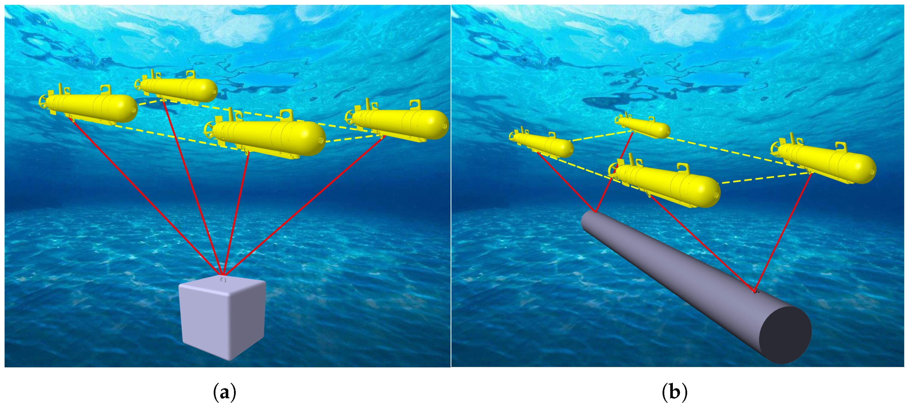
5.1. Multi-UUV Single Lifting Point Formation Transportation of a Payload

In this scenario, we establish a situation in which a multi-UUV (indices 1–4) formation cooperatively transports a payload (index 5) with single lifting in a 3-D obstacle space. To this end, the UUVs should first complete the desired formation and then achieve formation cooperative transport of a payload along a planned formation motion trajectory until the desired destination is reached. Figure 8 and Figure 9 display the simulated results of the first example. The resulting trajectories of formation maneuvers of four transport UUVs and one payload are shown in Figure 8, where the trajectory of the planned waypoint is marked by the red “+”, the trajectory of the payload is marked by the black “·”, the trajectories of UUVs are marked by the pink “·”, and the blue solid lines represent the formation configuration every 10 s. Figure 8a shows the 3-D trajectories, while Figure 8b shows 2-D (x–y plane). The smooth planned trajectory verified the ability of the IFF algorithm to plan obstacle avoidance path in complex obstacle spaces. The movement trajectory of the payload closely aligns with the intended route, indicating that the control algorithm exhibits good tracking performance for the planned trajectory. The formation always maintains a rigid structure, without collisions and with continuous paths, demonstrating the effectiveness of motion planning. Figure 8b shows that the formation naturally avoids obstacles along the “bypass flow” characteristics of the fluid (the path curvature continuously changes), conforms to the UUV maneuverability constraint (no sharp turns), and avoids actuator saturation. This indicates that the transport UUV formation can maneuver in formation in a multi-obstacle space to coordinate the transportation of payload.

Figure 9a shows the distance errors $e_{ij}\left(t\right),i,j\in {\mathcal{V}}^{*}$ for any two nodes, which converge rapidly to zero (within approximately 4 s), indicating that the formation control based on the rigidity graph achieves precise geometric constraints. Figure 9b denotes the control inputs ${\overline{\tau }}_i\left(t\right)$ of 4 UUVs in three coordinate directions, which fluctuates significantly in the initial stage (In response to the initial distance error, and the peak reflects the system inertia. These can be reduced by implementing input saturation without affecting stability, as the NN compensates for transient effects), and then approaches zero, which is in line with expectations. Once a stable formation is formed, only minor adjustments are needed to maintain the formation shape. Each output of the NN, and consequently each column of the weight matrix W, is related to a communication edge. Figure 9c presents the sample of NN weights W that are associated with node 1. The weights converge rapidly to the steady-state values, indicating that NN has effectively learned the compensation strategy for model uncertainty. Finally, Figure 9d shows the parameter estimates of the transport UUV labeled as 1, ${\widehat{\varphi }}_1$, indicating that the parameter estimates gradually reach and settle at stable values over time. The asymptotic convergence of the dynamic parameter estimates verifies the robustness of the adaptive law (49) against system uncertainties.

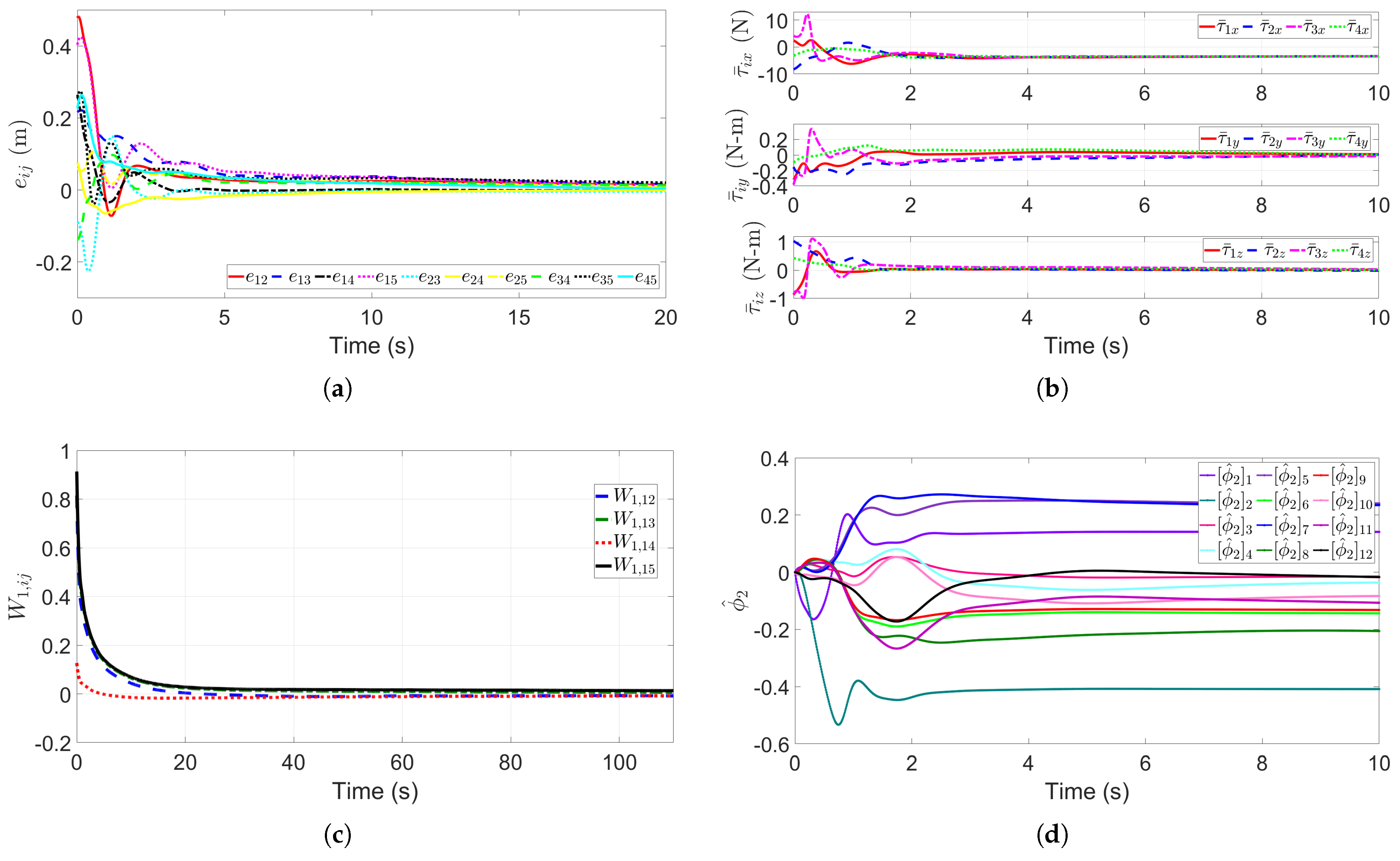
5.2. Multi-UUV Double Lifting Point Formation Transportation of a Payload

The simulation in this scenario is performed for the formation cooperative transport of a payload with double lifting in a 3-D space. Figure 10 shows the trajectories of the transport UUV and payload when passing through the obstacle space. As can be found in Figure 10a, all UUVs in formation can effectively avoid obstacles in the environment and navigate to the destination under the guidance of the planned motion trajectory. The trajectory navigates flexibly among the obstacles, as the complexity of the trajectory increases, it remains smooth, verifying the algorithm’s compatibility with the multi-hanging point topology. Figure 10b depicts the paths of formation and the final formation structure in the $xoy$-plane. The 2-D trajectories show the outline of the formation’s bypass obstacles, and the path curvature changes naturally, which conforms to the “bypass flow” characteristic of the fluid disturbance algorithm.

The position distance errors $e_{ij}\left(t\right),i,j\in {\mathcal{V}}^{*}$, as shown in Figure 11a, converge to zero. The convergence speed of the error is comparable to that of a single lifting point, indicating that the algorithm applies to different load connection methods. The formation control inputs ${\overline{\tau }}_i\left(t\right)$ of every UUV in the x, y and z coordinates are given in Figure 11b, which keep close to zeros after the formation is achieved, indicating that the double lifting points do not significantly increase the control burden. The simulation also shows that the suggested control technique may, through formation reconfiguration, ensure a secure voyage for multi-UUV systems in confined space. Figure 11c gives the sample of NN weights W corresponding to the node 1. Its convergence mode is consistent with that of a single hanging point, reflecting the generalization ability of NN. Figure 11d shows the parameter estimates of transport UUV labeled as 2, ${\widehat{\varphi }}_2$. The parameter estimates of different UUVs all converge, proving the universality of distributed control.

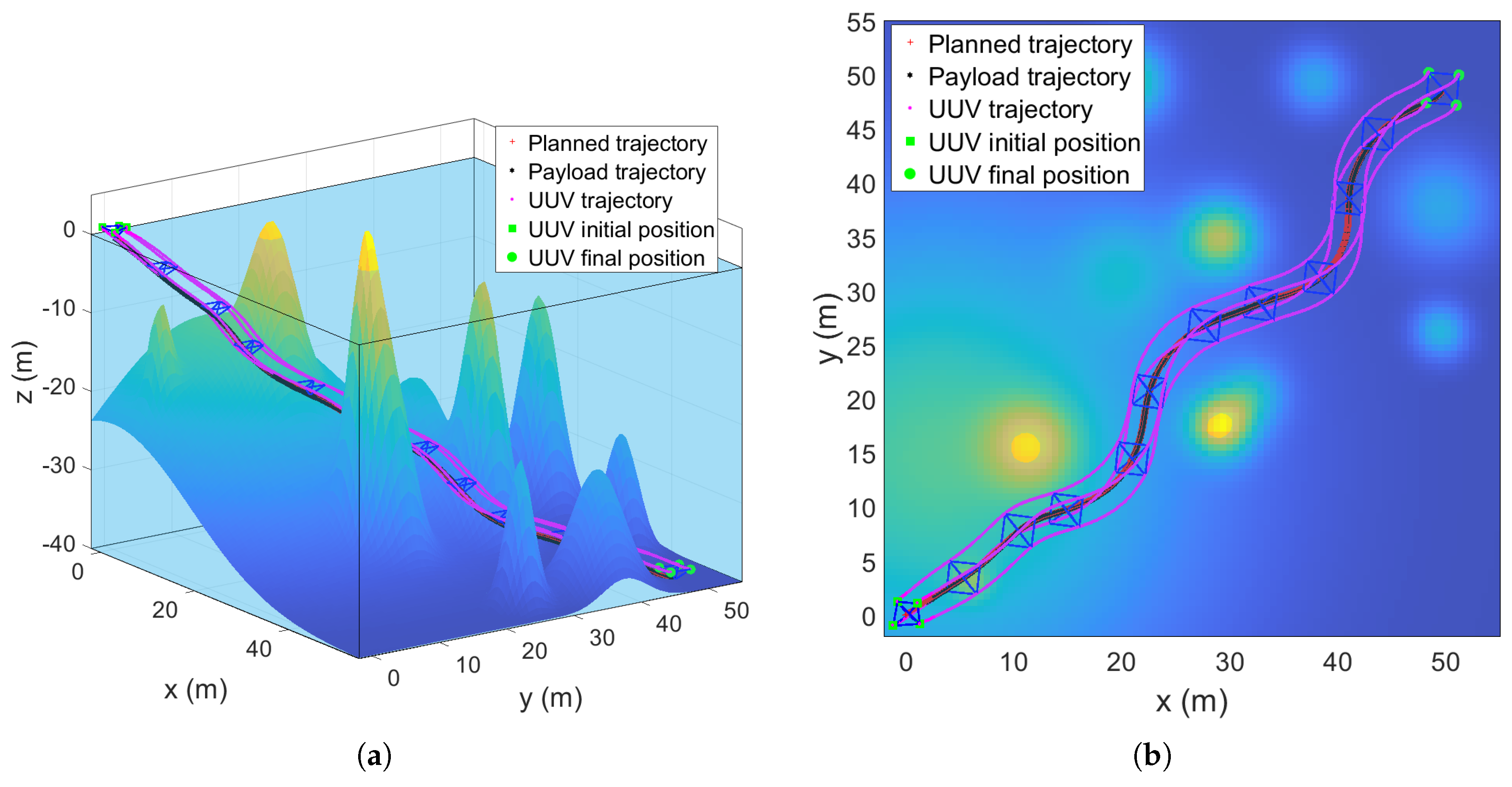
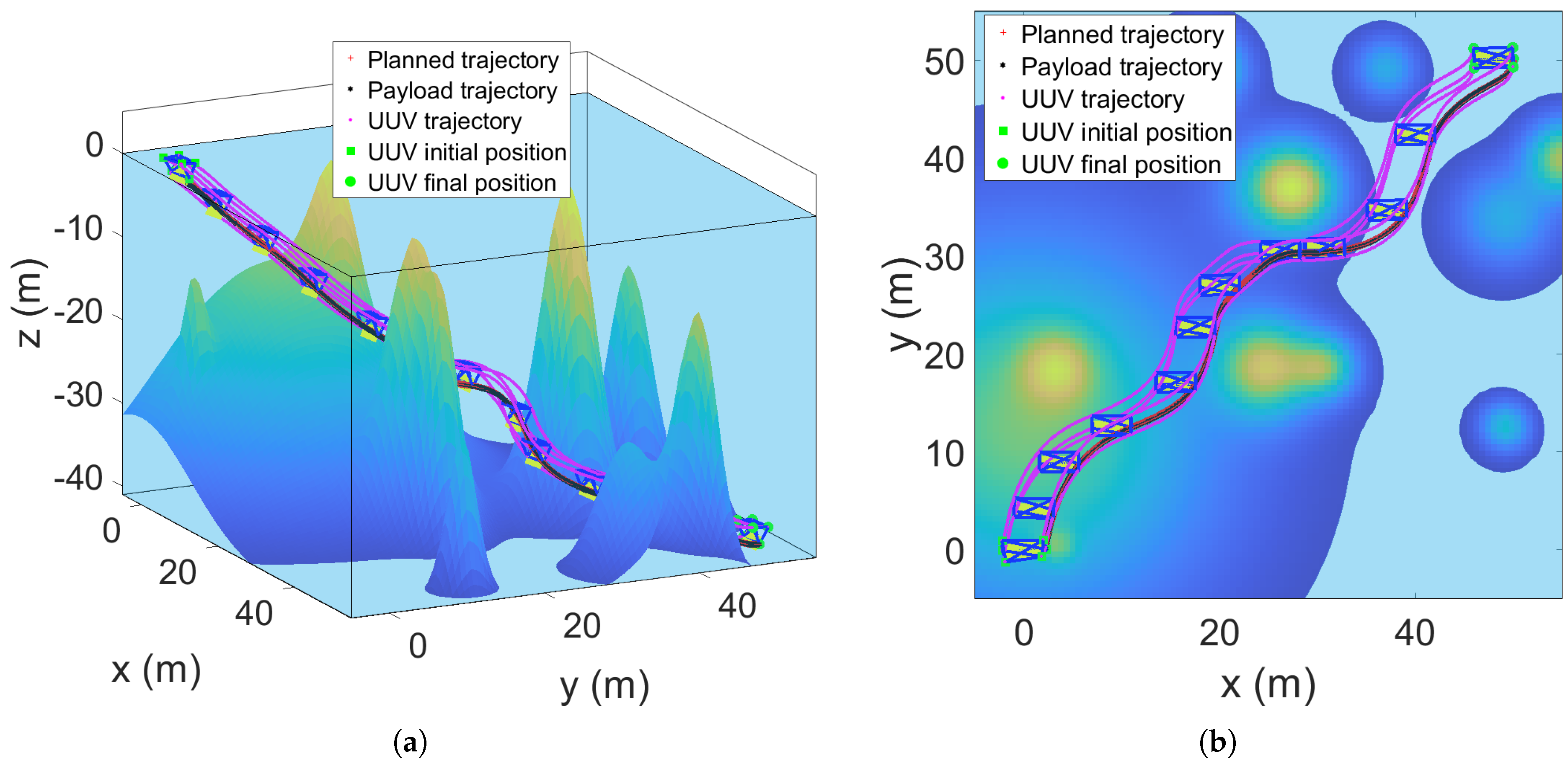
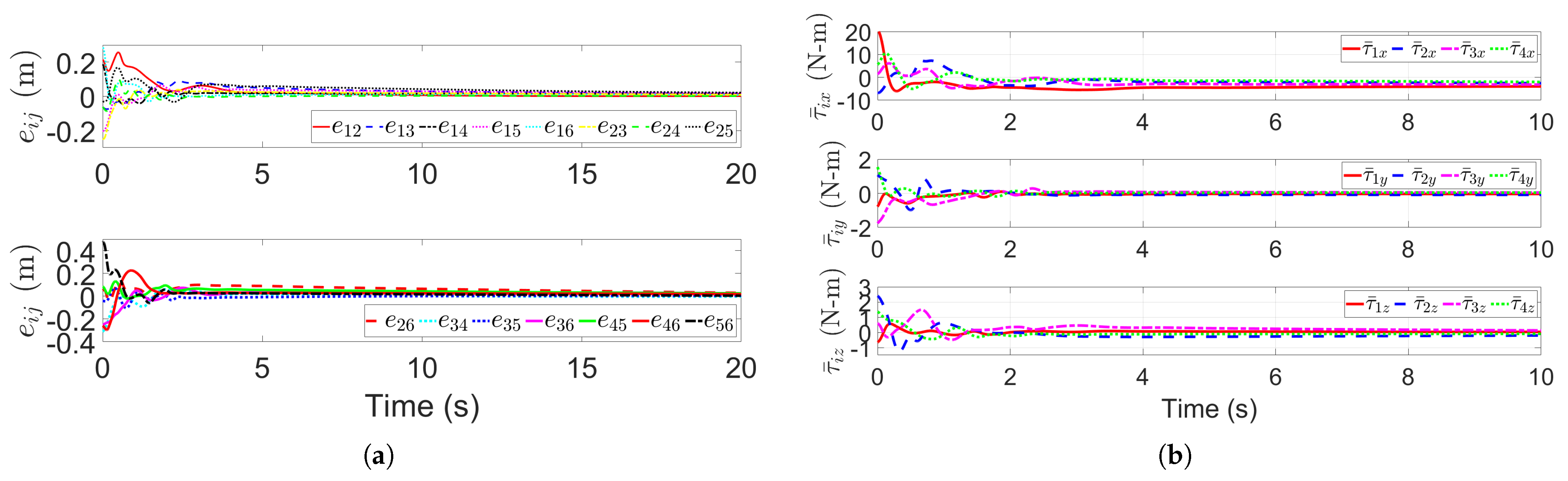
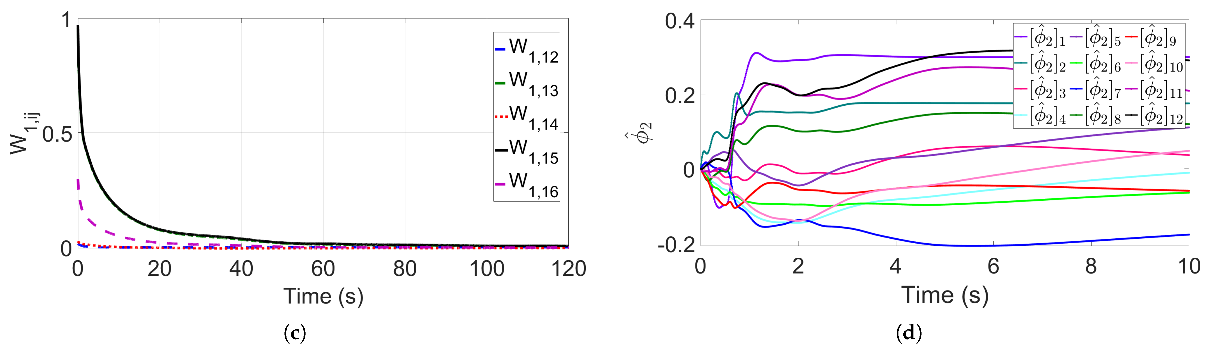
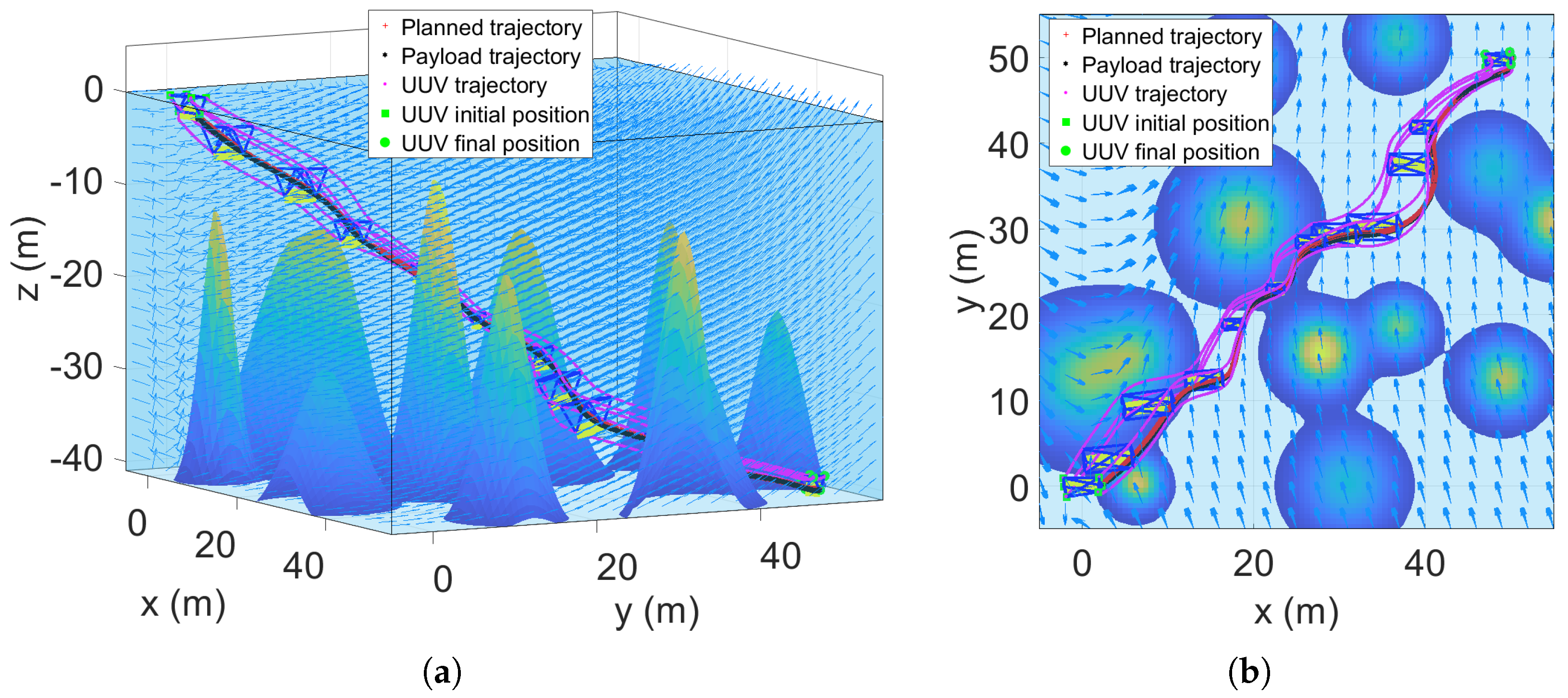
5.3. Multi-UUV Double Lifting Point Formation Transportation of a Payload in Dense Obstacle Environment Under External Disturbance

The simulation in this scenario is performed for the formation cooperative transportation of a payload with double lifting, where a 3-D space with dense obstacles and external disturbances is considered. In this scenario, additional obstacles are sintroduced, and if the UUV transport formation cannot pass through the obstacle area, the formation shape must be reconfigured to adapt to the situation. This is achieved via affine transformation [37], which enables formation reconfiguration through structure scaling. The distances between UUVs are autonomously regulated to reduce the formation size until a smaller configuration is achieved.

Figure 12 illustrates the motion trajectories of the formation scaling in a multi-obstacle environment. The results indicate that, even in complex environments with various obstacles and external disturbances, the transport UUV can navigate along the planned path by employing the design method in (46). Through formation scaling, the UUVs can effectively avoid obstacles and reliably and swiftly reach the target for payload delivery. Figure b depicts both the formation trajectories and the final formation structure on $xoy$-plane. This demonstrates that not only the achievement of an expected rigid formation but also the clear representation of the formation structure scaling process during payload transportation. Additionally, the collaborative robustness of the motion planning and control systems has been verified.

Figure 13a shows the distance errors $e_{ij}\left(t\right),i,j\in {\mathcal{V}}^{*}$. One can find that despite the existence of random interferences, the errors still converges to zero, proving the effectiveness of neural network perturbation compensation in (46). Figure 13b illustrates the control inputs ${\overline{\tau }}_i\left(t\right)$. Figure 13c,d present the random external disturbances and the parameter estimates of transport UUV labeled as 4, ${\widehat{\varphi }}_4$, respectively. The parameter estimates of all UUVs still converge stably under disturbances, highlighting the robustness of the adaptive law and reinforcing the conclusion of system stability.

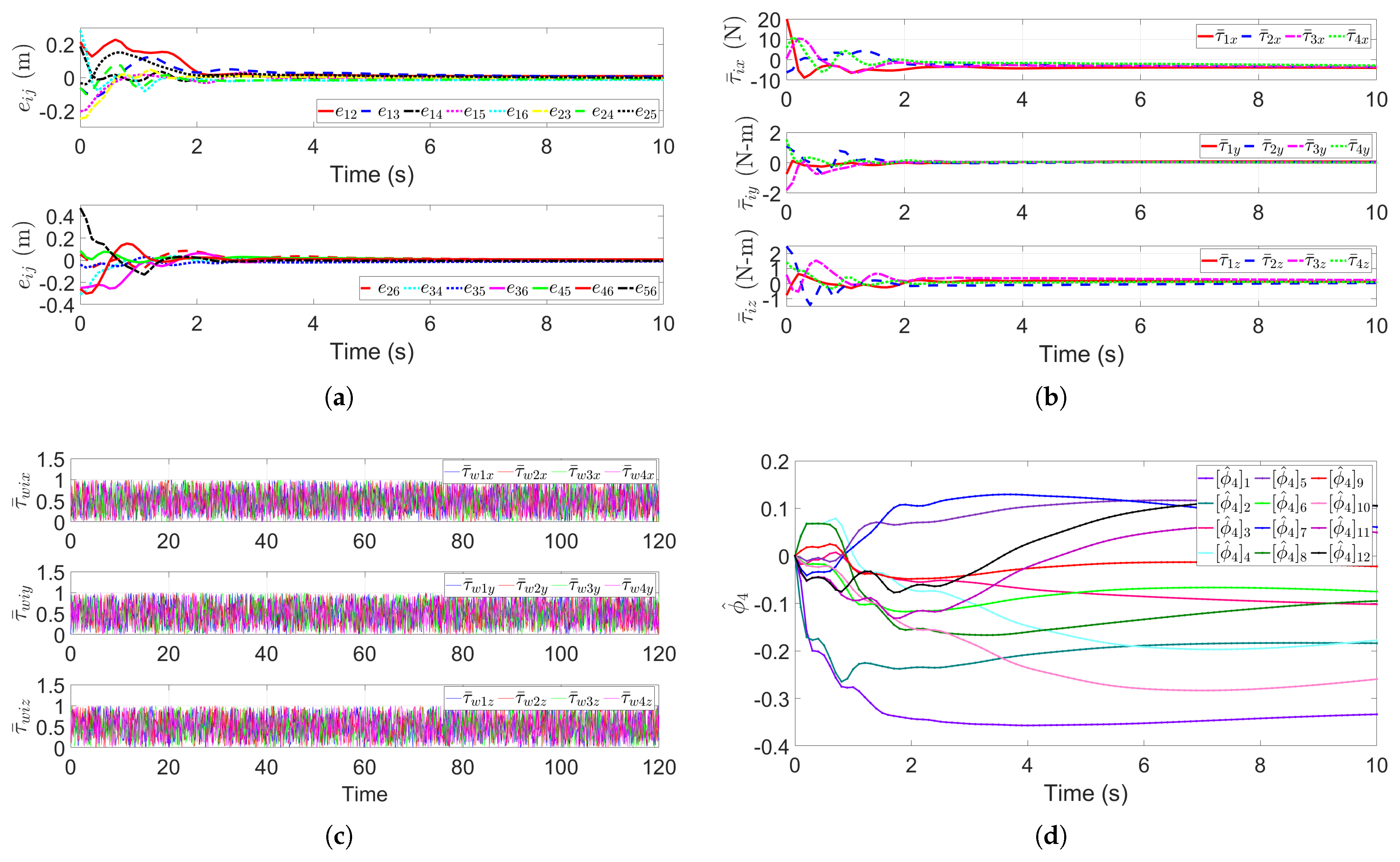
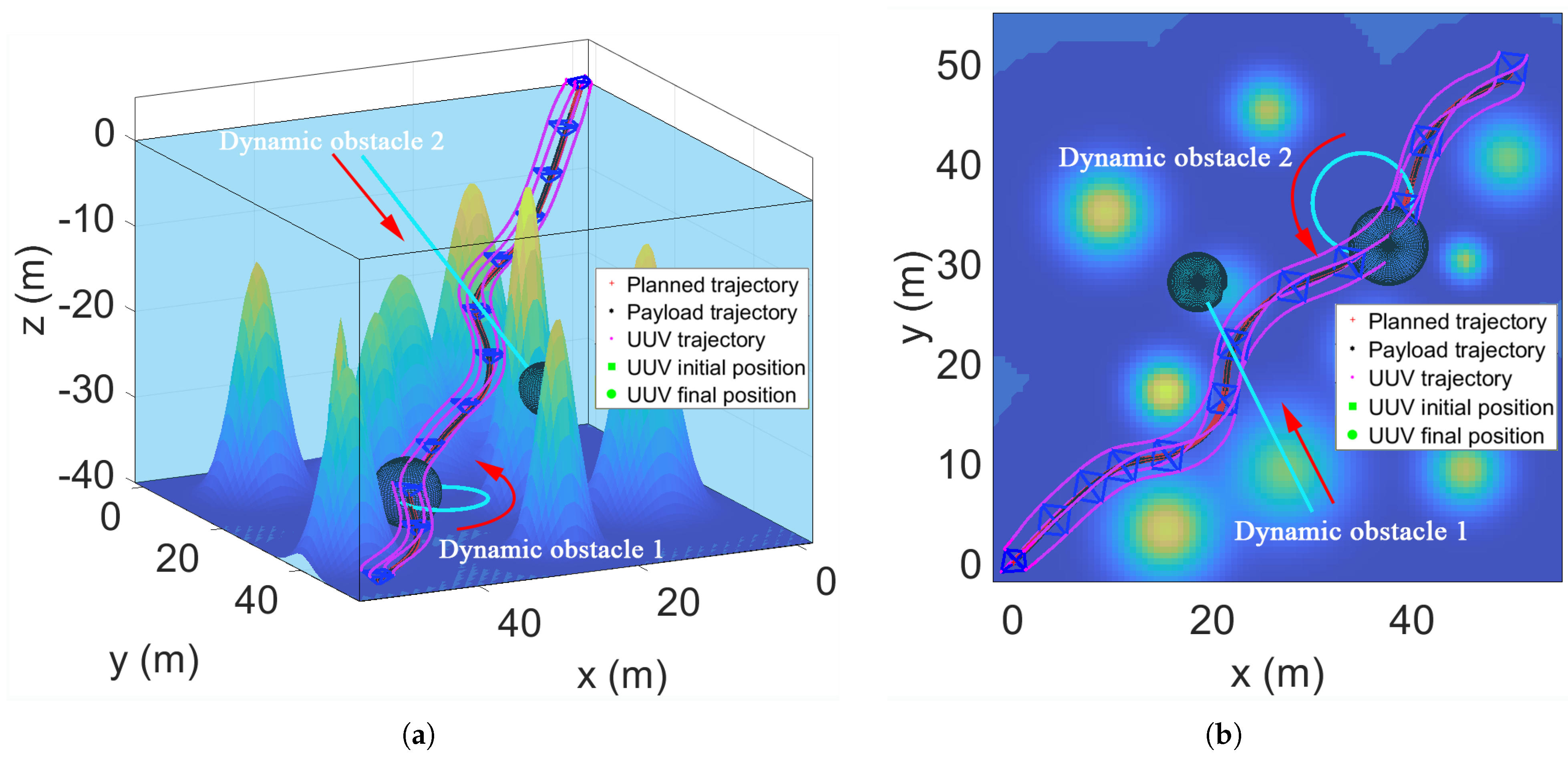
5.4. Multi-UUV Single Lifting Point Formation Transportation of a Payload in Dynamic Obstacle Environment

The simulation in this part is performed for the formation cooperative transport of a payload with single lifting in a 3-D space with dynamic obstacles. In this scenario, we have set up 10 static obstacles and 2 dynamic obstacles. The starting positions of the two dynamic obstacles are $p_{obs1}=(30,5,-3)$ and $p_{obs2}=(35,36,-35)$, respectively. Among them, dynamic obstacle 1 moves straight at a constant speed of $v_{obs1}=(-0.1,0.2,-0.2)$ m/s, and dynamic obstacle 2 moves in a circular motion with a speed of $v_{obs2}=(-0.5sin\left(0.1t\right),0.5cos\left(0.1t\right),0)$ m/s. The simulation results are presented in Figure 14 and Figure 15.

Figure 14 displays the trajectories of formation UUVs when passing through a dynamic obstacle environment, where Figure 14a shows the 3-D trajectories and Figure 14b presents 2-D trajectories on the x–y plane. The trajectory is locally adjusted in the dynamic obstacle area, but the whole remains smooth and continuous, verifying the real-time performance of the IFF algorithm in dynamic adjustment and verified the bionic characteristics of the IFF algorithm in naturally handling dynamic obstacles.

As shown in Figure 15a, the distance errors $e_{ij}\left(t\right),i,j\in {\mathcal{V}}^{*}$ between any two nodes in formation tend to zero. Figure 15b shows the control inputs ${\overline{\tau }}_i$ of all UUVs in the transport formation along the three coordinate axes. Figure 15c gives the sample of NN weights correspond to node 1, and Figure 15d shows the parameter estimates of transport UUV labeled as 2, ${\widehat{\varphi }}_2$.

Overall, the simulation results comprehensively verify the three major contributions of the paper and provide an innovative solution for underwater collaborative transportation.

6. Conclusions

This article focuses on the formation control and motion planning issues of cooperative transport of an underwater payload using multi-UUV systems. The designed controller can generate a smooth motion route for UUVs in the transport formation with complex obstacle-filled environments under external disturbances, which not only adheres to UUV maneuverability restrictions but also enables the UUVs to naturally bypass obstacles. Moreover, the proposed hybrid method features simplicity in principle, high computational efficiency, and strong practicality, which are all notable advantages. The corresponding simulation results demonstrate that the proposed controller can guide the UUV formation to avoid obstacles through formation reconfiguration. In this study, firstly, the positions of all obstacles were known. One of the future research directions is to extend the algorithm to randomly moving obstacles. Secondly, considering the load variations of each UUV and the tension distribution of the cable is a crucial issue. We plan to conduct research on this aspect using optimization algorithms [13] and more advanced neural networks in the future. Finally, since this algorithm has not been tested on physical platforms, we are developing an experimental platform to verify it.

References

1. Petillot, Y.R.; Antonelli, G.; Casalino, G.; Ferreira, F. Underwater Robots: From Remotely Operated Vehicles to Intervention-Autonomous Underwater Vehicles. IEEE Robot. Autom. Mag. 2019, 26, 94–101. [Google Scholar] [CrossRef]
2. Chen, M.; Zhu, D.; Pang, W.; Chen, Q. An Effective Strategy for Distributed Unmanned Underwater Vehicles to Encircle and Capture Intelligent Targets. IEEE Trans. Ind. Electron. 2024, 71, 12570–12580. [Google Scholar] [CrossRef]
3. Liu, H.; Wang, Y.; Lewis, F.L. Robust distributed formation controller design for a group of unmanned underwater vehicles. IEEE Trans. Syst. Man Cybern. Syst. 2021, 51, 1215–1223. [Google Scholar] [CrossRef]
4. Yang, Y.; Xiao, Y.; Li, T. A survey of autonomous underwater vehicle formation: Performance, formation control, and communication capability. IEEE Commun. Surv. Tutor. 2021, 23, 815–841. [Google Scholar] [CrossRef]
5. He, L.; Xie, M.; Zhang, Y. A Review of Path Following, Trajectory Tracking, and Formation Control for Autonomous Underwater Vehicles. Drones 2025, 9, 286. [Google Scholar] [CrossRef]
6. Wang, H.; Su, B. Event-triggered formation control of AUVs with fixed-time RBF disturbance observer. Appl. Ocean Res. 2021, 112, 102638. [Google Scholar] [CrossRef]
7. Yan, J.; Zhang, X.; Yang, X.; Chen, C.; Guan, X. Potential-Game-Driven Formation Control of AUVs: An Inverse-Reinforcement-Learning-Based Solution. IEEE J. Ocean. Eng. 2025, 50, 1165–1183. [Google Scholar] [CrossRef]
8. Wang, M.; Pang, S.; Jin, K.; Liang, X.; Wang, H.; Yi, H. Construction and experimental verification research of a magnetic detection system for submarine pipelines based on a two-part towed platform. J. Ocean Eng. Sci. 2023, 8, 169–180. [Google Scholar] [CrossRef]
9. Yu, H.; Ma, Y. A cooperative mission planning method considering environmental factors for UUV swarm to search multiple underwater targets. Ocean Eng. 2024, 308, 118228. [Google Scholar] [CrossRef]
10. Li, J.; Bian, X.; Huang, H.; Jiang, T.; Liu, Y.; Wan, L. Hybrid visual servoing control for underwater vehicle manipulator systems with multiple cameras. IEEE Trans. Syst. Man Cybern. Syst. 2024, 54, 1742–1754. [Google Scholar] [CrossRef]
11. Simetti, E.; Casalino, G. Manipulation and transportation with cooperative underwater vehicle manipulator systems. IEEE J. Ocean. Eng. 2017, 42, 782–799. [Google Scholar] [CrossRef]
12. Jin, X.; Hu, Z. Adaptive cooperative load transportation by a team of quadrotors with multiple constraint requirements. IEEE Trans. Intell. Transp. Syst. 2023, 24, 801–814. [Google Scholar] [CrossRef]
13. Zhang, X.; Zhang, F.; Huang, P. Formation planning for tethered multirotor UAV cooperative transportation with unknown payload and cable length. IEEE Trans. Autom. Sci. Eng. 2024, 21, 3449–3460. [Google Scholar] [CrossRef]
14. Heshmati-Alamdari, S.; Bechlioulis, C.P.; Karras, G.C.; Kyriakopoulos, K.J. Cooperative impedance control for multiple underwater vehicle manipulator systems under lean communication. IEEE J. Ocean. Eng. 2021, 46, 447–465. [Google Scholar] [CrossRef]
15. Heshmati-Alamdari, S.; Karras, G.C.; Kyriakopoulos, K.J. A predictive control approach for cooperative transportation by multiple underwater vehicle manipulator systems. IEEE Trans. Control Syst. Technol. 2022, 30, 917–930. [Google Scholar] [CrossRef]
16. De Oliveira, É.L.; Orsino, R.M.M.; Donha, D.C. Modular modeling and coordination control scheme for an underwater cooperative transportation performed by two I-AUVs. Control Eng. Pract. 2022, 125, 105198. [Google Scholar] [CrossRef]
17. Conti, R.; Meli, E.; Ridolfi, A.; Allotta, B. An innovative decentralized strategy for I-AUVs cooperative manipulation tasks. Robot. Auton. Syst. 2015, 72, 261–276. [Google Scholar] [CrossRef]
18. Pi, R.; Cieślak, P.; Ridao, P.; Sanz, P.J. Twinbot: Autonomous underwater cooperative transportation. IEEE Access 2021, 9, 37668–37684. [Google Scholar] [CrossRef]
19. Zhang, D.; Wang, L.; Yu, J.; Tan, M. Coordinated transport by multiple biomimetic robotic fish in underwater environment. IEEE Trans. Control Syst. Technol. 2007, 15, 658–671. [Google Scholar] [CrossRef]
20. Shao, J.; Wang, L.; Yu, J. Development of an artificial fish-like robot and its application in cooperative transportation. Control Eng. Pract. 2008, 16, 569–584. [Google Scholar] [CrossRef]
21. Bacelar, T.; Madeiras, J.; Melicio, R.; Cardeira, C.; Oliveira, P. On-board implementation and experimental validation of collaborative transportation of loads with multiple UAVs. Aerosp. Sci. Technol. 2020, 107, 106284. [Google Scholar] [CrossRef]
22. Zhao, W.; Xia, Y.; Zhai, D.H.; Sun, Z.; Zhang, Y. Event-Triggered Formation Control of Unknown Autonomous Underwater Vehicles Subject to Arbitrarily Large Time-Varying Communication Delays. IEEE Trans. Veh. Technol. 2025, 74, 3901–3912. [Google Scholar] [CrossRef]
23. Yao, M.; Yu, L.; Guo, K.; Lu, Y.; Zhang, W.; Qiao, L. Distributed Two-Layered Leader–Follower Affine Formation Control for Multiple AUVs in 3-D Space. IEEE Trans. Syst. Man Cybern. Syst. 2025, 55, 85–95. [Google Scholar] [CrossRef]
24. Yan, J.; Wu, C.; Yang, X.; Chen, C.; Guan, X. Minimum Time Formation Control of AUVs with Smooth Transition in Communication Topology. IEEE Robot. Autom. Lett. 2024, 9, 8698–8705. [Google Scholar] [CrossRef]
25. Hadi, B.; Khosravi, A.; Sarhadi, P. Adaptive formation motion planning and control of autonomous underwater vehicles using deep reinforcement learning. IEEE J. Ocean. Eng. 2024, 49, 311–328. [Google Scholar] [CrossRef]
26. Shojaei, K. Neural adaptive PID formation control of car-like mobile robots without velocity measurements. Adv. Robot. 2017, 31, 947–964. [Google Scholar] [CrossRef]
27. Rani, M.; Kumar, N. A neural network based efficient leader–follower formation control approach for multiple autonomous underwater vehicles. Eng. Appl. Artif. Intell. 2023, 122, 106102. [Google Scholar] [CrossRef]
28. Wang, H.; Lyu, W.; Yao, P.; Liang, X.; Liu, C. Three-dimensional path planning for unmanned aerial vehicle based on interfered fluid dynamical system. Chin. J. Aeronaut. 2015, 28, 229–239. [Google Scholar] [CrossRef]
29. Celestini, D.; Primatesta, S.; Capello, E. Trajectory planning for UAVs based on interfered fluid dynamical system and Bézier curves. IEEE Robot. Autom. Lett. 2022, 7, 9620–9626. [Google Scholar] [CrossRef]
30. Wu, J.; Wang, H.; Li, N.; Su, Z. Formation obstacle avoidance: A fluid-based solution. IEEE Syst. J. 2019, 14, 1479–1490. [Google Scholar] [CrossRef]
31. Niu, Y.; Yan, X.; Wang, Y.; Niu, Y. 3D real-time dynamic path planning for UAV based on improved interfered fluid dynamical system and artificial neural network. Adv. Eng. Inform. 2024, 59, 102306. [Google Scholar] [CrossRef]
32. Tamanakijprasart, K.; Mondal, S.; Tsourdos, A. Dynamic path planning of UAV in three-dimensional complex environment based on interfered fluid dynamical system. In Proceedings of the AIAA SCITECH 2024 Forum, Orlando, FL, USA, 8–12 January 2024. [Google Scholar] [CrossRef]
33. Li, X.; Wen, C.; Chen, C. Adaptive formation control of networked robotic systems with bearing-only measurements. IEEE Trans. Cybern. 2021, 51, 199–209. [Google Scholar] [CrossRef] [PubMed]
34. Aryankia, K.; Selmic, R.R. Neural network-based formation control with target tracking for second-order nonlinear multiagent systems. IEEE Trans. Aerosp. Electron. Syst. 2022, 58, 328–341. [Google Scholar] [CrossRef]
35. Do, K.D.; Pan, J. Control of Ships and Underwater Vehicles: Design for Underactuated and Nonlinear Marine Systems; Springer Science and Business Media: Berlin/Heidelberg, Germany, 2009. [Google Scholar]
36. Paliotta, C.; Lefeber, E.; Pettersen, K.Y.; Pinto, J.; Costa, M. Trajectory tracking and path following for underactuated marine vehicles. IEEE Trans. Control Syst. Technol. 2018, 27, 1423–1437. [Google Scholar] [CrossRef]
37. Pang, W.; Zhu, D.; Chu, Z.; Chen, Q. Distributed adaptive formation reconfiguration control for multiple AUVs based on affine transformation in three-dimensional ocean environments. IEEE Trans. Veh. Technol. 2023, 72, 7338–7350. [Google Scholar] [CrossRef]
38. Anderson, B.D.; Yu, C.; Fidan, B.; Hendrickx, J.M. Rigid graph control architectures for autonomous formations. IEEE Control Syst. Mag. 2008, 28, 48–63. [Google Scholar]
39. Pang, W.; Zhu, D.; Sun, C. Multi-AUV Formation Reconfiguration Obstacle Avoidance Algorithm Based on Affine Transformation and Improved Artificial Potential Field Under Ocean Currents Disturbance. IEEE Trans. Autom. Sci. Eng. 2024, 21, 1469–1487. [Google Scholar] [CrossRef]
40. Lewis, F.L.; Jagannathan, S.; Yeşildirek, A. Neural network control of robot arms and nonlinear systems. In Neural Systems for Control; Academic Press: Cambridge, MA, USA, 1997; pp. 161–211. [Google Scholar]
41. Khalil, H.K. Nonlinear Systems; Prentice Hall: Upper Saddle River, NJ, USA, 2002. [Google Scholar]
Figure 1. Cooperative transportation and delivery task conducted by formation of UUVs in a 3-D obstacle environment.
Drones 09 00465 g001
Figure 2. 3-D configuration of ith transport UUV.
Drones 09 00465 g002
Figure 3. Some approximation of typical convex solid obstacles.
Drones 09 00465 g003
Figure 4. The planning trajectories obtained by IFF with different parameters ρ and σ . (a) Increase parameter ρ . (b) Increase parameter σ .
Drones 09 00465 g004
Figure 5. Origin flow lines and interfered flow lines in a complex 3-D obstacle space. (a) Original streamlines. (b) Modified streamlines.
Drones 09 00465 g005
Figure 6. Block diagram of multi-UUV cooperative transportation formation control and trajectory planning.
Drones 09 00465 g006
Figure 7. Schematic of cooperative transportation of underwater payload by multiple UUVs. (a) Single lifting point transport. (b) Double lifting point transport.
Drones 09 00465 g007
Figure 8. Movement trajectories of formation cooperative underwater payload transport and delivery with single lifting point. (a) 3-D view. (b) 2-D (xy) view.
Drones 09 00465 g008
Figure 9. (a) The errors e i j ( t ) , i , j V * in the distance separating any pair of nodes. (b) The formation control input τ ¯ i for each transport UUV in x, y and z directions. (c) Sample of NN weights W 1 , i j . (d) Sample of parameters estimates for UUV 1, ϕ ^ 1 .
Drones 09 00465 g009
Figure 10. Movement trajectories of formation cooperative underwater payload transport and delivery with with double lifting point. (a) 3-D view. (b) 2-D (xy) view.
Drones 09 00465 g010
Figure 11. (a) The distance errors e i j ( t ) , i , j V * between any pair of nodes. (b) The formation control inputs τ ¯ i for each transport UUV in x, y and z directions. (c) Sample of NN weights W 1 i j . (d) Sample of parameters estimates for UUV 2, ϕ ^ 2 .
Drones 09 00465 g011aDrones 09 00465 g011b
Figure 12. Movement trajectories of formation cooperative underwater payload transport and delivery with double lifting point in a dense obstacle environment under external disturbance. (a) 3-D view. (b) 2-D (xy) view.
Drones 09 00465 g012
Figure 13. (a) The distance errors e i j ( t ) , i , j V * between any two nodes. (b) The formation control inputs τ ¯ i for each transportion UUV in x, y and z directions. (c) Random external disturbances τ ¯ w i along the three coordinate axes. (d) Sample of parameters estimates for UUV 4, ϕ ^ 4 .
Drones 09 00465 g013
Figure 14. Movement trajectories of formation cooperative underwater payload transport and delivery with single lifting point in a dynamic obstacle environment. (a) 3-D view. (b) 2-D (xy) view.
Drones 09 00465 g014
Figure 15. (a) The distance errors e i j ( t ) , i , j V * between any two nodes. (b) The formation control inputs τ ¯ i for each transportation UUV in x, y and z directions. (c) Sample of NN weights W 1 , i j . (d) Sample of parameters estimates for UUV 2, ϕ ^ 2 .
Drones 09 00465 g015