Article

Cooperative Networked Quadrotor UAV Formation and Prescribed Time Tracking Control with Speed and Input Saturation Constraints

1
College of Information Engineering, Henan University of Science and Technology, Luoyang 471023, China
2
Henan Key Laboratory of Robot and Intelligent Systems, Henan University of Science and Technology, Luoyang 471023, China
3
School of Automation Science and Electrical Engineering, Beihang University, Beijing 100083, China
4
College of Agricultural Equipment Engineering, Henan University of Science and Technology, Luoyang 471023, China
*
Author to whom correspondence should be addressed.
Drones 2025, 9(6), 417; https://doi.org/10.3390/drones9060417
Submission received: 5 May 2025 / Revised: 28 May 2025 / Accepted: 6 June 2025 / Published: 8 June 2025

Abstract

:
This paper addresses the challenges of cooperative formation control and prescribed-time tracking for networked quadrotor UAVs under speed and input saturation constraints. A hierarchical control framework including position formation layer and attitude tracking layer is proposed, which achieves full drive control of an underactuated UAV formation system by introducing the expected tracking Euler angle. For the outer-loop position control, a distributed consensus protocol with restricted state and control inputs is designed to ensure formation stability with customizable spacing and bounded velocity. The inner-loop attitude control employs a prescribed-time sliding mode attitude controller (PTSMAC) integrated with a prescribed-time extended state observer (PTESO), enabling rapid convergence within user-defined time and compensating for unmodeled dynamics, wind disturbances, and actuator saturation. The effectiveness of the proposed algorithm was demonstrated through Lyapunov stability. Comparative simulations show that the proposed method has significant advantages in high-precision formation control, convergence time, and input saturation.

1. Introduction

In recent years, the cooperative control of multi-UAV systems has emerged as a research hot spot in the field of intelligent unmanned systems, propelled by rapid advancements of UAV technology and its broad application prospects in both civil and military fields. Quadrotor UAV, characterized by its high maneuverability, flexible formation capabilities, and cost-effectiveness, have played irreplaceable role in civilian applications such as agricultural plant protection [1], load transportation [2], and traffic data collection [3], as well as military tasks like area surveillance [4] and collaborative strikes [5]. However, as a typical research subject, the formation control of quadrotor UAVs is confronted with multiple challenges, including strong nonlinear coupling, complex environmental disturbances, and physical constraints, which severely restrict the dynamic performance and mission reliability of UAV formations. Consequently, there is an urgent need to develop robust and efficient cooperative control methods to enable UAVs to stably and efficiently execute tasks in diverse complex scenarios.
Nevertheless, with regard to quadrotor UAVs, as a classic highly-coupled under-actuated system, most existing studies in formation control predominantly adopt the hierarchical control framework for multi-UAV systems to decouple translational dynamics and rotational dynamics. For instance, ref. [6] designs a distributed active disturbance rejection formation control scheme, the position loop constructs a distributed tracking law based on neighboring UAV position information and introduces a distributed adaptive observer to estimate the yaw angle of leader, while the attitude loop employs a cascaded active disturbance rejection controller and uses extended state observer (ESO) to estimate tracking errors in real time. Aiming at scenarios with sensor limitations, ref. [7] designs a disturbance observer in the position loop to estimate disturbances and combines sliding-mode control to handle position errors, the attitude loop uses a second-order sliding surface to suppress chattering, and relies only on measurable position and attitude angles, reducing dependence on velocity sensors. With growing attention to model uncertainties, adaptive mechanisms have been introduced. Ref. [8] proposes neural adaptive control for nonlinear and unmodeled dynamics, the position subsystem approximates nonlinearities using the RBF NNs scheme and constructs a second-order sliding surface to handle trajectory errors, while the attitude subsystem designs a full-order observer to estimate unmeasurable states. To tackle actuator faults, ref. [9] applies saturation control in the position loop to bound command thrust and avoid actuator saturation, while the attitude loop uses projection adaptive techniques to online estimate the inertia matrix and designs controllers for Euler angles and angular velocity. For complex tasks, hierarchical control has been further integrated with intelligent algorithms. Ref. [10] proposes a multi-layer neural dynamics controller, where the outer layer constructs a time tracking error function based on neural dynamics to achieve time-varying position tracking through multi-level error feedback, and the inner layer adapts parameters to compensate for mass estimation errors, enhancing robustness to time-varying tasks. Ref. [11] combined with reinforcement learning, designs an outer layer containment control strategy that models pursuit–evasion games via Markov decision processes and an inner layer critic-only NN to approximate optimal control laws, achieving Nash equilibrium in adversarial scenarios. However, this hierarchical control has inherent inter-layer coupling issues—especially when the response frequencies of the position layer and attitude layer are similar, which exacerbates the coupling and leads to degraded control performance. An effective approach to address this problem is to shorten the convergence time of the attitude loop and enhance the response frequency of the inner loop.
The convergence time of formation control scheme is a critical evaluation index to determine the efficiency of executing time-urgent flight missions, especially in scenarios such as emergency rescue and military coordination. Finite-time, fixed-time, and prescribed-time control methods have attracted significant attention from researchers due to their unique advantages. Ref. [12] introduced a fixed-time error observer to counteract unmodeled wind disturbances and designed a robust guidance law based on this observer, enabling UAV formations to track targets within finite time. However, this study did not account for the impact of stochastic disturbances, which cannot all be precisely modeled. Therefore, ref. [13] treats UAVs as stochastic systems and designs a finite-time fuzzy backstepping controller, by employing terminal sliding mode technology to construct a rapidly converging sliding surface and integrating fuzzy logic to approximate unknown nonlinear dynamics, it ensures that position and attitude errors converge within finite time. To eliminate the dependence of convergence time on initial states in finite-time control, fixed-time control-based cooperative formation control methods are widely proposed. In practical applications, UAV formation often required to complete their configuration within fixed time. Ref. [14] proposes a fixed-time formation containment control scheme, which uses a distributed architecture and a dual-power-term control law to guarantee followers enter the convex hull spanned by the leader within a fixed time, even with significant initial positional deviations. For multi-UAV formation control under actuator faults while ensuring collision avoidance, ref. [15] designs a fixed-time sliding-mode controller that integrates the gradient of repulsive potential functions into the sliding surface to calculate real-time safety distances and generate obstacle avoidance forces, while compensating for actuator failures through fault observers. Ref. [16] proposes a fixed-time sliding mode control method within the leader–follower framework, ensuring that all states converge in a fixed time. Nevertheless, the convergence time of fixed-time control still requires indirect parameter tuning, prompting further research into more flexible predefined-time control. Prescribed-time control introduces time-varying scaling functions to reduce initial feedback gains and achieve user-specified time convergence of state variables. In the context of UAV actuator faults, ref. [17] designs a PTESO combined with prescribed performance functions to real-time estimate the effects of faults and disturbances, strictly constraining position and attitude errors within prescribed ranges and ensuring convergence within user-specified time. In our previous study [18], we integrated disturbance observers with predefined-time control for UAV trajectory tracking. By employing a control law with a time-scaling mechanism, the system compensates for unknown disturbances in real time, guaranteeing desired control performance for single quadrotor UAV. This work establishes a solid foundation for our subsequent work.
In addition to convergence time constraints, UAV control faces multiple challenges including actuator saturation, model parameter uncertainties, unknown disturbances, and physical limitations, which have inspired targeted solutions through research across different dimensions. Actuator output saturation represents the primary performance-limiting factor for UAV. Ref. [19] proposes a saturation-adaptive sliding mode control that characterizes input constraints through piecewise saturation functions and incorporates adaptive control laws for online gain adjustment, ensuring actual control inputs remain within predefined safety bounds. Ref. [20] constructs auxiliary equations to approximate saturation characteristics, transforming saturated inputs into continuous controllable forms to avoid nonlinear saturation-induced stability issues. For model parameter uncertainties and unknown disturbances, ref. [21] leverages the strong robustness of global sliding mode control by treating disturbances as extended states in sliding surface design. Through constructing a nonlinear sliding surface that includes the integral of virtual control inputs, it guarantees finite-time convergence of system states. Ref. [22] introduces a state compensation function observer combined with a tracking differentiator to real-time estimate dynamic disturbance changes, using feedforward compensation to counteract disturbances in advance and accurately estimate wind disturbances and model uncertainties. Focusing on the active suppression of unknown wind disturbances, ref. [23] develops a joint framework of two-stage particle filter and nonsingular terminal sliding mode control, enabling real-time estimation and compensation of wind effects without relying on precise wind field models. UAVs also face physical boundary challenges such as speed limits and communication constraints in practical missions. Addressing speed and input constraints in multi-agent systems, ref. [24] embeds a weighted neighbor state error mechanism into saturation control laws and applies fixed-time stability theory to strictly ensure the speeds and control inputs of each UAV do not exceed physical limits. For communication constraints in multi-UAV collaboration, ref. [25] models dynamic communication topologies using Markov jump networks and employs virtual information sharing with fault-tolerant algorithms to ensure collaborative control under uncertain network connections, achieving generalized Nash equilibrium in multi-UAV systems. Ref. [26] proposes a three-dimensional cooperative guidance method for sensor-constrained scenarios.
For the challenges in UAV formation control, including inter-layer coupling, physical constraints, unmodeled errors, and unknown wind disturbances, this paper proposes a hierarchical cooperative and disturbance-robust prescribed-time formation control method that integrates distributed consensus protocols, ESO, PTESO, and PTSMAC.
The principal contributions are encapsulated in the following facets:
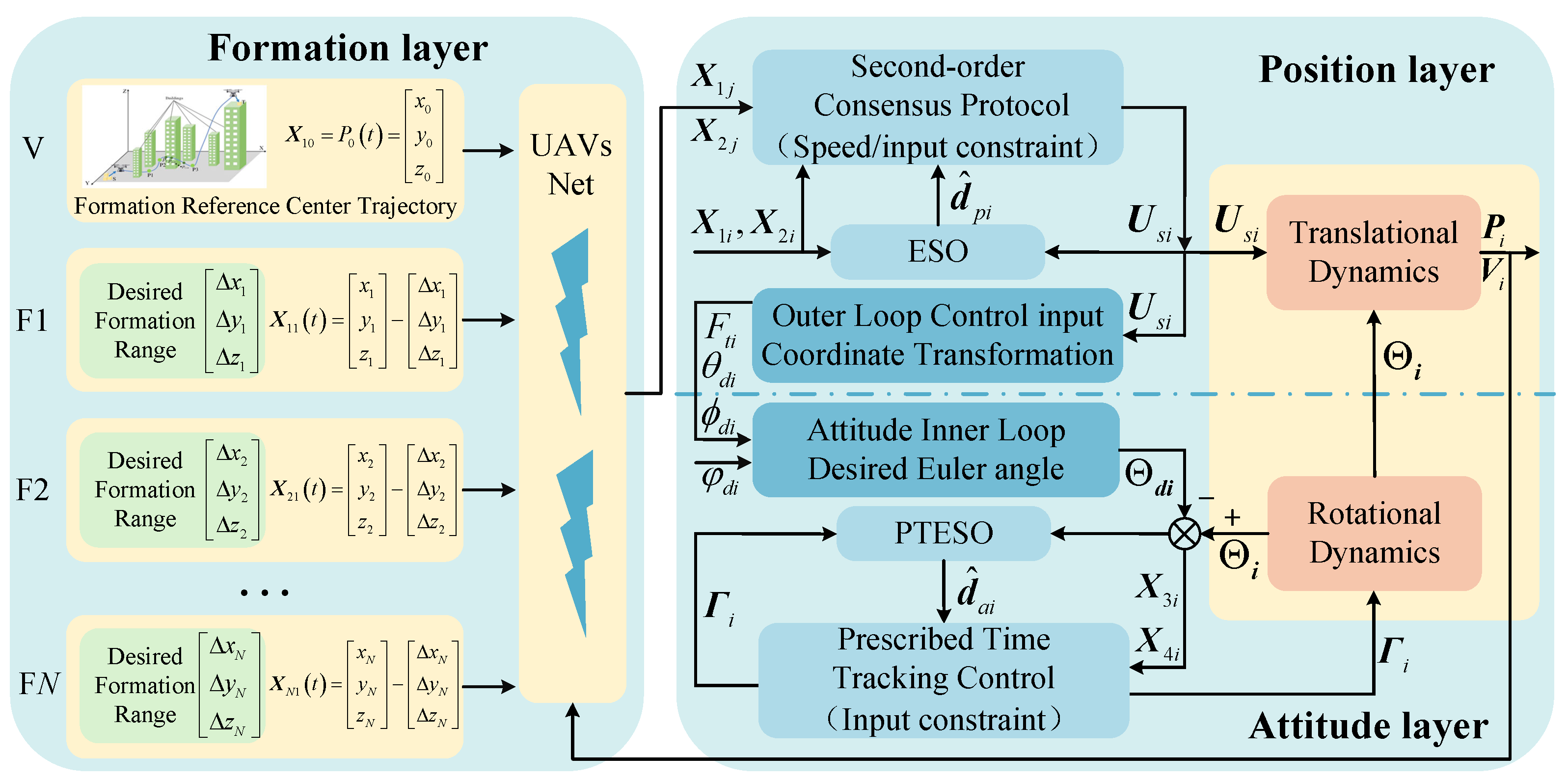
  • This study tackles the state coupling issue between the position outer loop and attitude inner loop in UAV formation control, which is exacerbated when the response frequencies of both loops are comparable. For the position outer loop, a distributed consensus protocol is designed to guarantee the position stability of the UAV formation. The attitude inner loop employs prescribed-time control strategy, which enables the arbitrary setting of the convergence speed of the inner loop, enhances the response speed of the inner loop relative to the outer loop, and reduces the spectral coupling effect between the inner and outer loops.
  • To handle constraints on UAV velocity, attitude, torque, and other related control variables, a second-order consensus protocol is devised with velocity and input constraints, which is used to design a formation outer-loop controller that can impose constraints on the UAV speed and desired Euler angle. Furthermore, a continuous saturation function is introduced to design a PTSMAC with control input constraints, which can achieve prescribed-time convergent tracking control of attitude commands under constrained control inputs.
  • For disturbance rejection against unmodeled errors, unknown wind disturbances, and other factors, an ESO is utilized in the outer-loop position control to ensure the robustness of disturbance estimation. In the attitude loop, a PTESO is adopted. By setting consistent convergence time parameters in both PTESO and PTSMAC, a less conservative control strategy is realized for the inner-loop attitude controller.
The rest of this paper is organized as follows: In Section 2, some preliminaries and the problem formulation are given. Section 3 introduces the proposed distributed control strategy and the design of the attitude controller. The simulation results verifying the proposed method and comparing it with another method are described in Section 4. Finally, Section 5 concludes this paper and suggests future research directions.

2. Preliminaries and Problem Formulation

2.1. Mathematical Model

This paper concerns the formation and attitude tracking control of N quadrotor UAVs. The structure of UAVs is shown in Figure 1. The UAV utilizes four rotors to facilitate its six degrees of freedom (DOF) in motion, with each UAV being independently controlled by a brushless DC motor. To describe the translational motion (position loop) and rotational motion (attitude loop) of the UAV, an earth inertial coordinate frame and a body coordinate frame are defined, respectively, as illustrated in Figure 1. Similarly, the mathematical model of any UAV can be represented as a position subsystem and an attitude subsystem.
The 6 DOF model of UAV i is as follows
x ¨ i = ( C ϕ i S θ i C ψ i + S ϕ i S ψ i ) F 1 i m k x i m x ˙ i + d x u i y ¨ i = ( C ϕ i S θ i S ψ i S ϕ i C ψ i ) F 1 i m k y i m y ˙ i + d y u i z ¨ i = ( C ϕ i C θ i ) F 1 i m g i k z i m z ˙ i + d z u i ϕ ¨ i = θ ˙ i ψ ˙ i I y I z I x I r I x θ ˙ i ω ¯ k ϕ i I x ϕ ˙ i + 1 I x τ ϕ i + d ϕ u i θ ¨ i = ϕ ˙ i ψ ˙ i I z I x I y I r I y ϕ ˙ i ω ¯ k θ I y θ ˙ i + 1 I y τ θ i + d θ u i ψ ¨ = ϕ ˙ i θ ˙ i I x I y I z k ψ i I z ψ ˙ i + 1 I z τ ψ i + d ψ u i
where S ( · ) and C ( · ) represent sin · and cos · , respectively.
(1)
The translational dynamics:
P ˙ i = V i , V ˙ i = g + 1 m i R b i e u p i + d p i , i = 1 , 2 , , N .
where P i = [ x i , y i , z i ] T is the position coordinate of UAV i in the earth inertial system, V i = [ V x i , V y i , V z i ] T represents the velocity vector, g = [ 0 , 0 , g ] T is the gravity acceleration component of the UAVs on different coordinate axes in inertial system, u p i = [ 0 , 0 , F t i ] T is the control input of the position loop, d p i = [ d x i , d y i , d z i ] T = 1 m K p i V i + d p u i is a comprehensive unknown disturbance, where K p i = d i a g k x i , k y i , k z i are drag coefficients, which are associated with the flight speed, altitude, air temperature, and other factors of UAVs. These coefficients cannot be obtained in practical systems and are challenging to accurately measure through experiments. Consequently, the drag term constituted by these coefficients is treated as an unknown disturbance. Furthermore, unknown variables d p u i = d x u i , d y u i , d z u i T are introduced to represent the unknown wind disturbances and other unmodeled dynamics. R b i e is the the coordinate transformation matrix from the body frame to the earth inertial frame, which is defined as
R b i e = C θ i C ψ i S ϕ i S θ i C ψ i C ϕ i S ψ i C ϕ i S θ i C ψ i + S ϕ i S ψ i C θ i S ψ i S ϕ i S θ i S ψ i + C ϕ i C ψ i C ϕ i S θ i S ψ i S ϕ i C ψ i S θ i S ϕ i C θ i C ϕ i C θ i
Remark 1. 
It is worth noting that the state vectors within the translational dynamics depicted in Equation (2) are situated in three-dimensional space. However, among the three-dimensional control vectors, only the total thrust F t i is controllable. To achieve full state control of three-dimensional translational motion, it is a common strategy to introduce pitch and roll angles as intermediate control variables. This allows for the position control of the UAV through the coordination of thrust and attitude angles. Therefore, this paper selects u s i = [ Q x i , Q y i , Q z i ] T as the intermediate control variable in the position loop within the inertial frame.
Q x i = ( C ϕ i S θ i C ψ i + S ϕ i S ψ i ) F t i Q y i = ( C ϕ i S θ i S ψ i S ϕ i C ψ i ) F t i Q z i = ( C ϕ i C θ i ) F t i
Taking the yaw angle ψ i as a known value, based on the designed u s , the desired attitude angle ϕ d i , θ d i can be obtained, as well as the total pulling force F t i of the UAV i is designed.
F t i = u s i = Q x i 2 + Q y i 2 + Q z i 2 ϕ d i = arcsin Q x i S ψ i Q y i C ψ i u s i θ d i = arctan Q x i C ψ i + Q y i S ψ i Q z i
(2)
The rotational dynamics:
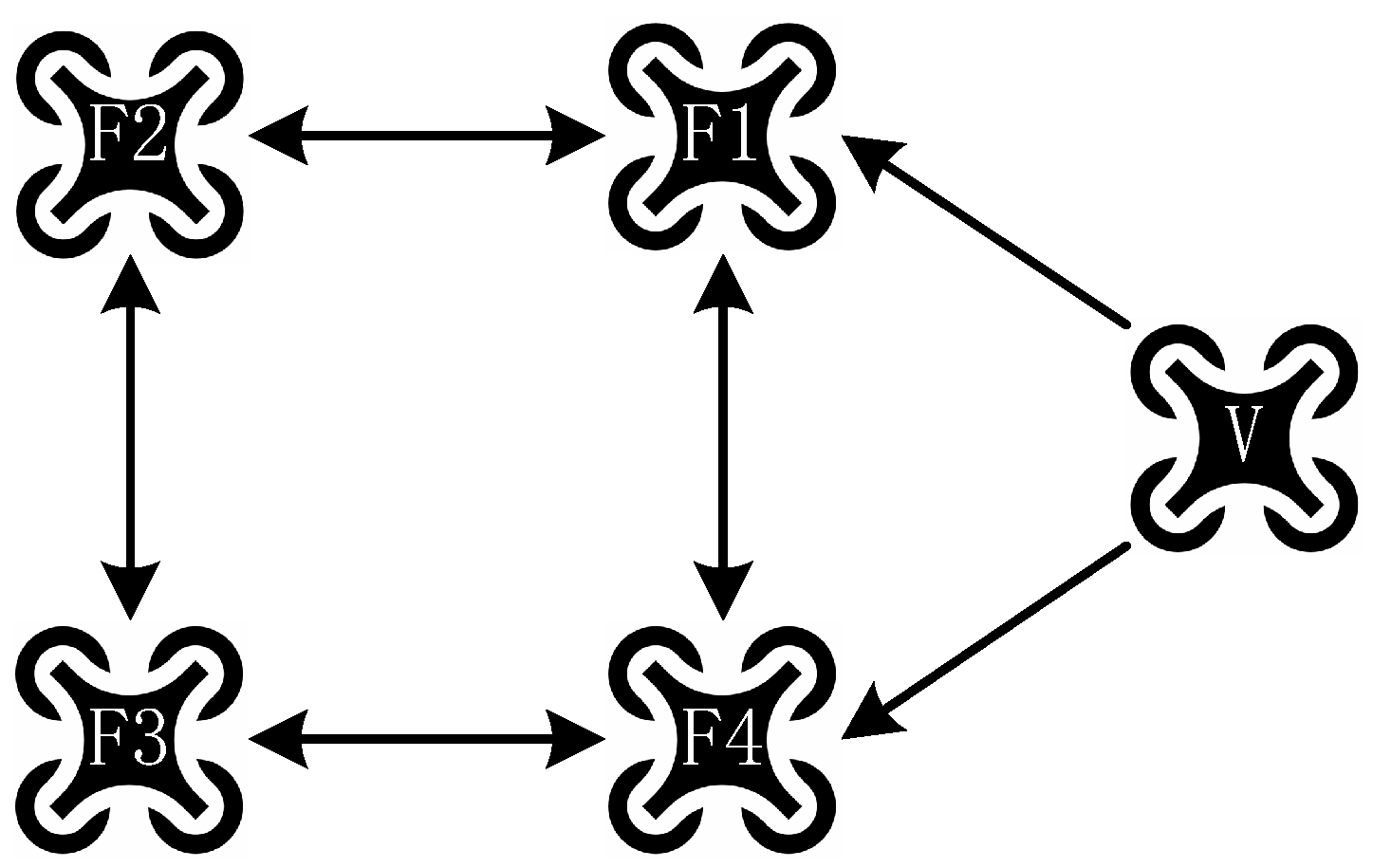
Θ ˙ i = Ω i , Ω ˙ i = J i 1 G a , i + J i 1 Γ a i + d a , i , i = 1 , 2 , , N .
where G a , i = θ ˙ i ψ ˙ i I y I z , ϕ ˙ i ψ ˙ i I z I x , ϕ ˙ i θ ˙ i I x I y T , Θ i = ϕ i , θ i , ψ i T , Ω i = ϕ ˙ i , θ ˙ i , ψ ˙ i T , J i = diag I x , I y , I z , Γ i = τ ϕ i , τ θ i , τ ψ i T are the attitude control moments, d a i = [ d ϕ 0 i , d θ 0 i , d ψ 0 i ] T = J 1 K a i Ω i + d Δ ω i + d a u i is a comprehensive unknown disturbance in attitude loop, K a i = diag k ϕ i , k θ i , k ψ i is the damping torque coefficient matrix, d Δ ω i = I r I x θ ˙ i ω ¯ i , I r I y ϕ ˙ i ω ¯ i , 0 T , d a u i = d ϕ u i , d θ u i , d ψ u i T denotes the other disturbance torque caused by the unknown wind and other unmodeled dynamics. Besides, ω ¯ i = ω 2 i + ω 4 i ω 1 i ω 3 i is the speed difference that generates yaw moment in the plane of UAsV i.
Remark 2. 
In the attitude subsystem, the control inputs of the UAV are selected as three control torques τ ϕ i , τ θ i , τ ψ i , combined with the control input F t i selected by the translational subsystem, to form the control vector of the UAV system. The quadrotor UAV is controlled by four independent motors, with their rotational speeds denoted as ω 1 i , ω 2 i , ω 3 i , ω 4 i , respectively. For a × type UAV, as shown in Figure 1, the relationship between rotational speed and corresponding torque is as follows:
F t i τ ϕ i τ θ i τ ψ i = c T c T c T c T 2 2 l c T 2 2 l c T 2 2 l c T 2 2 l c T 2 2 l c T 2 2 l c T 2 2 l c T 2 2 l c T c M c M c M c M ω 1 i 2 ω 2 i 2 ω 3 i 2 ω 4 i 2
where l is the UAV arm length, c T and c M represent the lift and torque coefficient, respectively.
Assumption 1. 
The communication topology graph among the UAVs is directed and contains a spanning tree.
Assumption 2. 
The disturbance in the UAV attitude loop is unknown bounded, and the maximum available control input of the attitude loop is greater than the maximum error of the observer in estimating the disturbance.

2.2. Graph Theory

In the UAV formation control problem studied in this paper, each UAV is regarded as an agent. Algebraic graph theory serves as an important analytical tool for describing the connection relationships among agents. The communication relationship between UAVs is denoted as a graph G = { V , E , A } , where V = { V 1 , V 2 , , V n } is the set of N UAVs, E = e i j V × V i , j = 1 , 2 , , N is the set of edge, A = { a i j } denotes the adjacency matrix. If there is information flowing from UAV j to UAV i, a i j = 1 , otherwise, a i j = 0 . Specially, the diagonal elements of the adjacency matrix are all 0, that is, a i i = 0 . The degree matrix is defined as D = diag { d 1 , d 2 , , d n } , where d i = j = 1 n a i j is the in-degree of node i. The Laplace matrix is denoted as L = D A .

2.3. Some Lemmas

Lemma 1 
([27]). Considering a dynamic system as q ˙ = f ( t , q ( t ) ) , where q t R m , if V ˙ ( t , q ( t ) ) satisfy
V ˙ ( t , q ( t ) ) b V k φ t 0 , T V ( t , q ( t ) )
Then, the following result can be obtained with t t 0 , t 0 + T
V μ t 0 , T k exp b t t 0 V t 0
where b > 0 ,   k > 0 are the constant parameters; φ t 0 , T and μ ( t 0 , T ) are the time-varying functions, which are defined as
φ t 0 , T = μ ˙ t 0 , T μ t 0 , T , t t 0 , t 0 + T p T , o t h e r w i s e
μ t 0 , T = T p t 0 + T t p , t t 0 , t 0 + T 1 , o t h e r w i s e
The time differential of the above functions are
φ ˙ t 0 , T = φ 2 t 0 , T p , t t 0 , t 0 + T 0 , o t h e r w i s e
μ ˙ t 0 , T = p T μ t 0 , T 1 + 1 p , t t 0 , t 0 + T 0 , o t h e r w i s e
Lemma 2 
([28]). For a following second-order system
x ˙ 1 = x 2 x ˙ 2 = f + b u + d
where x 1 and x 2 denote the system states, f and b are the known function, u represents the control input, d is the unknown bounded and smooth disturbance, d ˙ d ˙ max with d ˙ max being a constant. The disturbance can be estimated on the prescribed moment by the following PTESO
φ 1 = x 1 x ^ 1 x ^ ˙ 1 = x ^ 2 + T ζ Ξ ¯ l 1 φ 1 + ( 1 T ) k 1 Γ 1 3 φ 1 2 3 x ^ ˙ 2 = f + b u + d ^ + T ζ 2 Ξ ¯ 2 l 2 φ 1 + ( 1 T ) k 2 Γ 2 3 φ 1 1 3 d ^ ˙ = T ζ 3 Ξ ¯ 3 l 3 φ 1 + ( 1 T ) k 3 Γ φ 1 0
where Ξ ¯ = s e c 2 π 2 t t ¯ f , ζ is a positive constant, t 0 , t ¯ f and t ¯ f is the prescribed convergence time for the PTESO; Γ d ˙ max is a Lipschitz constant; l 1 , l 2 , l 3 , k 1 , k 2 , k 3 are the positive observer parameters, which satisfies k 3 > Γ , k 1 = 3.34 k 3 1 3 , and k 2 = 5.3 k 3 2 3 ; and T is the time switching function of the PTESO, which satisfies
T = 1 , t 0 , t ¯ f 0 , t t ¯ f , +
Lemma 3 
([29]). For a positive continuous function V ( x ) , if the time derivative of the function satisfies V ˙ ( x ) α V p β V q , where α , β > 0 , p > 1 , 0 < q < 1 . Then the state variable x can converge to 0 before the fixed-time T, the upper bound of convergence time can be estimated by T 1 α p 1 + 1 β 1 q .

3. Main Results

In this section, formation control is divided into three layers: formation, position, and attitude. Figure 2 shows the framework of the distributed formation and tracking controller for multi-UAV system.
  • At the formation layer, the distance from each UAV to the reference trajectory is determined based on a predefined performance function, which yields the state variable of the multi-agent consensus protocol. This provides a foundational model for formation design.
  • At the position layer, a distributed second-order multi-agent consensus protocol is utilized, which takes into account speed and input constraints. The reference trajectory acts as a virtual leader, allowing for consensus formation control among distributed, networked UAVs.
  • At the attitude layer, the designed control input for the position loop is inversely computed to set the desired Euler angles for the attitude inner loop. A prescribed time sliding mode controller with input constraints ensures rapid and stable tracking control.

3.1. Formation Strategy

The development of the distributed formation strategy involves two key components. First, an independently controlled leader UAV acts as the root node of the communication topology, ensuring compliance with Assumption 1. A consensus protocol is then created, allowing the follower UAVs to follow the leader consistently.
Then, unlike the traditional consensus problem, the UAVs maintain a specific formation rather than converging to a same value. This paper achieves UAV formation range control by designing the functions Δ x / y / z i ( t ) for i = 1 , 2 , , N . The formation spacing function is inspired by a preset performance control method, which is designed as
Δ ( t ) = Δ 0 Δ exp ( σ t ) ( T t ) l T l + Δ , 0 < t < T Δ , t T
where σ is a positive constant, l is a positive convergence rate parameter, T denotes a prescribed formation converge time, Δ 0 , and Δ are represent the initial and terminal formation distance for UAVs, respectively.

3.2. Distributed Formation Controller

Based on the formation strategy outlined above, the design goals for the position layer controller are as follows:
  • The trajectory of all UAVs should follow and navigate around the leader, with customizable formation spacing.
  • The designed formation controller must be robust against model uncertainties and unknown disturbances.
  • The convergence time of the controller should be as fast as possible to facilitate the rapid formation of UAV formation.
According to the translational dynamics and the formation control goals, the coordination variable for the UAVs are set as X 1 i = P i Δ i = x 1 i , y 1 i , z 1 i T , X 2 i = V i Δ ˙ i = v 2 x i , v 2 y i , v 2 z i T , where Δ i = Δ x i , Δ y i , Δ z i i = 1 , 2 , N . Additionally, X 10 = P 0 , X 20 = V 0 refers to the reference tracking trajectory for the UAV formation. By combining with Equation (2), the following kinematic model for multi-UAV cooperative formation can be derived:
X ˙ 1 i = X 2 i X ˙ 2 i = U s i + e d p i
where U s i = Q x , Q y , Q z g T + d ^ p i = u x i , u y i , u z i T is the control input to be designed. d ^ p i is a disturbance compensation item, which is obtained from an ESO designed as Lemma 2.3 in [30]. e d p i = d p i d ^ p i = e x d p i , e y d p i , e z d p i T is the disturbance estimate error, which is bounded and the upper boundary is denoted as τ max . Considering the UAV flight speed and control input is limited, the proposed controller must satisfy the following constraints:
X 2 i t V max , U s i t U max
where U max and V max are the given positive constant vector, and the initial speed of all the UAVs are in the given range.
In the translational motion control of UAV formations, the three-dimensional components of state vectors X 1 i exhibit mutual independence, allowing for independent channel-wise design. Based on this characteristic, this paper selects the x-axis as a typical example to elaborate the systematic design process of the formation controller. It is noted that the design methodologies for y-axis and z-axis UAV formation controllers maintain strict consistency with the x-axis, and thus will not be reiterated later.
To enhance clarity, the position and velocity error variables in x-axis are define as η x i = j = 1 n a i j x 1 i x 1 j and ζ x i = j = 1 n a i j v 2 x i v 2 x j , respectively. To ensure the speed of the UAV remains bounded, a saturation function is introduced to design the tracking reference speed r x i for UAVs i as
r i η i = m , if η i 4 m 3 k i 2 k i η i 3 4 m k i 2 η i 2 m 3 , if 2 m 3 k i η i < 4 m 3 k i k i η i , if 2 m 3 k i η i < 2 m 3 k i 2 k i η i + 3 4 m k i 2 η i 2 + m 3 , if 4 m 3 k i η i < 2 m 3 k i m , if η i 4 m 3 k i .
Further, the speed tracking error is define as e x i = v 2 x i r x i , and propose a distributed formation controller as follows:
u i = u max α i σ e i + λ i α i sgn e i λ i
where, λ i = z i γ i with γ i > 1 . Besides, z i , α i and m are positive constant satisfy Equation (22), σ e x i is a piecewise function designed as
σ e i = λ i s i g n e i , if   e i z i e i γ i s i g n e i , if   e i < z i
Theorem 1. 
Consider a multiple UAV system with N quadrotor UAVs. Assume that the communication topology graph G among the UAVs contains a directed spanning tree and the controller parameter satisfy in Equation (22). The proposed distributed formation controller Equation (20) ensures that the distance between the distributed UAVs (following UAVs) and the reference trajectory (virtual leading UAV) converges to the formation range Δ x i in x-axis. Additionally, it satisfies the constraints on UAV speed and control input outlined in Equation (18).
τ max < α i < u max m < v max z i v max m k i < α i τ max / 2 d i v max
Proof of Theorem 1. 
The proof of Theorem 1 is presented in Appendix A. □
Similarly, by applying Theorem 1 and controller Equation (20), the sub control inputs u y i , u z i for formation controller U s i in the y-axis and x-axis directions can also be obtained, respectively.

3.3. Attitude Controller
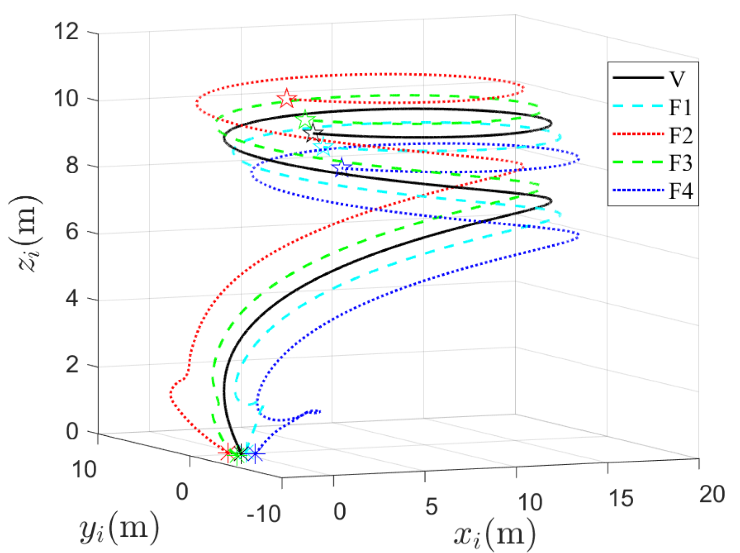
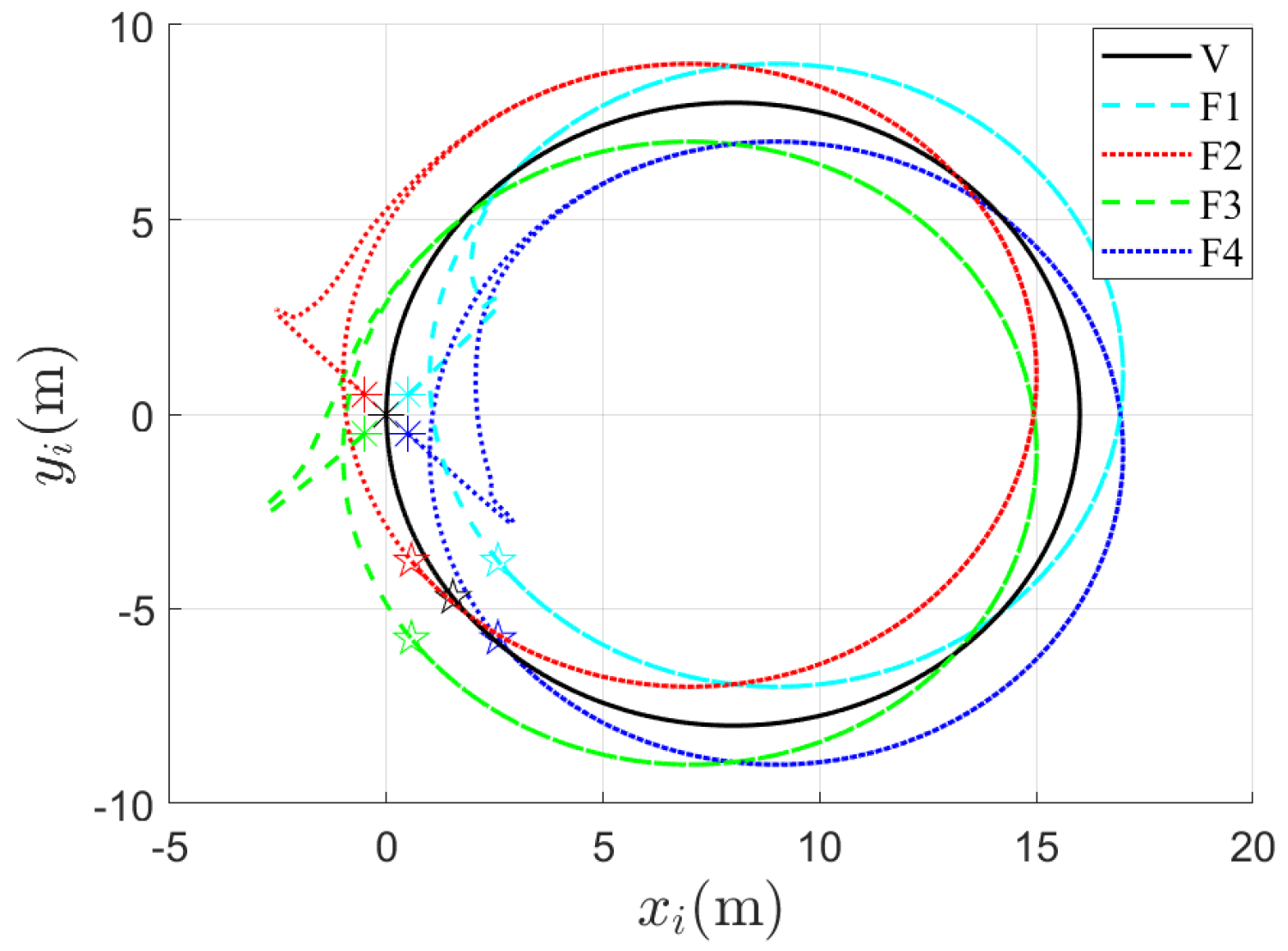
In this subsection, the quadrotor UAV inner loop controller is designed to ensure that the Euler angles Φ i = ϕ i , θ i , ψ i , T converge to the desired value Φ d i = ϕ d i , θ d i , ψ d i T within the prescribed time T a and ensures that the control input (torque for the UAV) Γ i = τ ϕ i , τ θ i , τ ψ i T not greater than the set range. Here, define the errors between the real and desired values of Euler angles as X 3 i = [ ϕ i ϕ d i , θ i θ d i , ψ i ψ d i ] T , the angle rates error is defined as X 4 i = [ ϕ ˙ i ϕ ˙ d i , θ i ˙ θ ˙ d i , ψ ˙ i ψ ˙ d i ] T .
Then, according to Equation (1), the error dynamic equation can be formulated as follows:
X ˙ 3 i = X 4 i X ˙ 4 i = f Φ i + B Φ i Γ i + d Φ i
where f Φ i = θ ˙ i ψ ˙ i I y I z I x , ϕ ˙ i ψ ˙ i I z I x I y , ϕ ˙ i θ ˙ i I x I y I z T , B Φ i = diag 1 I x , 1 I y , 1 I z , d Φ i = [ d ϕ i , d θ i , d ψ i ] T , Γ i = τ ϕ i , τ θ i , τ ψ i T .
Considering that the control torque of the UAV is limited in practice, a nonlinear saturation function s a t ( · ) is used in the attitude loop controller design to limit the amplitude of the control variable, which is designed as
τ θ i = s a t τ ˜ θ i = s i g n τ ˜ θ i τ θ max , τ ˜ θ i τ θ max τ ˜ θ i , τ ˜ θ i < τ θ max
Subsequently, the attitude dynamic equation Equation (23) can be rewritten as follows:
X ˙ 3 i = X 4 i X ˙ 4 i = f Φ i + B Φ i s a t Γ ˜ i + d Φ i
where Γ ˜ i = τ ˜ ϕ i , τ ˜ θ i , τ ˜ ψ i T is the saturation input for the attitude subsystem.
Considering that the saturation function s a t ( · ) is discontinuous, using the hyperbolic tangent function h ( τ ˜ j i ) ( j = ϕ , θ , ψ ) to approximate Equation (24) as follows:
h τ ˜ j i = τ j max tanh τ ˜ j i τ j max = τ j max e τ ˜ j i τ ˜ j i τ j max τ j max e τ ˜ j i τ ˜ j i τ j max τ j max e τ ˜ j i τ ˜ j i τ j max τ j max + e τ ˜ j i τ ˜ j i τ j max τ j max
where τ j max is the maximum amplitude limit of the control input for the three channels of the attitude subsystem.
According to Equations (25) and (26), the approximation error term is
Δ τ ˜ j i = s a t τ ˜ j i h τ ˜ j i
As the saturation function and hyperbolic tangent function are both bounded, the approximation error is also bounded as Δ τ ˜ j i = s a t τ ˜ j i h τ ˜ j i τ j max 1 tanh 1 .
By using Lagrange’s mean value theorem [31] for h τ ˜ j i , one can obtain that
h τ ˜ j i = h τ ˜ j i τ ˜ j i | τ ˜ j i = τ ˜ j i μ i τ ˜ j i
where τ ˜ j i μ i = μ i τ ˜ j i + 1 μ i τ ˜ j i 0 , μ i 0 , 1 .
Next, define the following matrix
H τ ˜ j i = diag h τ ˜ ϕ i τ ˜ ϕ i | τ ˜ ϕ i = τ ˜ ϕ i μ i h τ ˜ θ i τ ˜ θ i | τ ˜ θ i = τ ˜ θ i μ i h τ ˜ ψ i τ ˜ ψ i | τ ˜ ψ i = τ ˜ ψ i μ i
Then, the attitude model of quadrotor UAVs with input saturation constraint is as follows:
X ˙ 3 i = X 4 i X ˙ 4 i = f Φ i + B ˜ Φ i Γ ˜ i + d ˜ Φ i
where B ˜ Φ i = B Φ i H τ ˜ j i , d ˜ Φ i = B Φ i Δ τ ˜ j i + d Φ i is a comprehensive disturbance, Δ τ ˜ j i = Δ τ ˜ ϕ i , Δ τ ˜ θ i , Δ τ ˜ ψ i T is regarded as an unknown disturbance component.
The attitude loop, serving as the inner loop of the UAV formation control system, requires faster convergence speed. Therefore, by introducing the time-varying scaling function given in Equation (9), this paper designs the following prescribed-time convergent sliding mode attitude controller. To ensure that the system states x 3 i and x 4 i converge to 0 within a prescribed time T q , the following prescribed time convergence sliding mode surface is designed:
S i = x 4 i + c 1 + c 2 φ T a s , T a x 3 i
where c 1 > 0 , c 2 > 0 are the parameters for the slide mode surface; T a s denotes the desired convergence time for the slide mode surface S i . Additionally, the desired convergence time for the system states x 3 i and x 4 i is denoted as T a . To ensure that the system states x 3 i , x 4 i converge to the sliding mode surface at the prescribed time T a s , the following reaching law is designed:
S ˙ i = c 3 + c 4 φ T d a , T a s S i η 1 s i g n S i
where c 3 > 0 , c 4 > 0 , η 1 > 0 are the parameters of the reaching law.
By deriving Equation (31) and combining Equation (32), the attitude controller of UAV i with limited torque constraint can be designed as follows:
Γ i = h Γ ˜ i Γ ˜ i = B ˜ Φ i 1 f Φ i + d ^ Φ i + c 1 + c 2 φ T a s , T a x 3 i + c 2 φ ˙ T a s , T a x 2 i + c 3 + c 4 φ T d a , T a s S i + η 1 s i g n S i
where d ^ Φ i is the disturbance estimate value obtained by a PTESO, which is designed based on Lemma 2. T d a is the convergence time for the PTESO.
Theorem 2. 
For the attitude tracking control model of the pitching channel with the control input torque constraint, as shown in Equation (30), the unknown disturbance d ˜ Φ i is estimated by using the designed PTESO shown in Equation (14). Then the proposed prescribed time attitude controller Equation (33) can ensure that the system attitude angle and angular rate errors converge to 0 within the prescribed time T a , as well as the designed control input torque τ θ i , does not exceed the given range.
Proof of Theorem 2. 
The proof of Theorem 2 is presented in Appendix B. □

4. Simulation

To verify the performance of the proposed method, numerical simulation results of position/attitude tracking control of the multi-UAVs system and comparison with other methods are presented in this section. Consider a team of 5 networked quadrotor UAVs, consisting of one leader labeled by V and four followers labeled by F1 to F4. Figure 3 describes the directed communication topology among the leader and follower UAVs. Table 1 shows the physical parameters, unknown disturbance parameters, and unmodeled dynamics parameters of UAVs in this simulation.

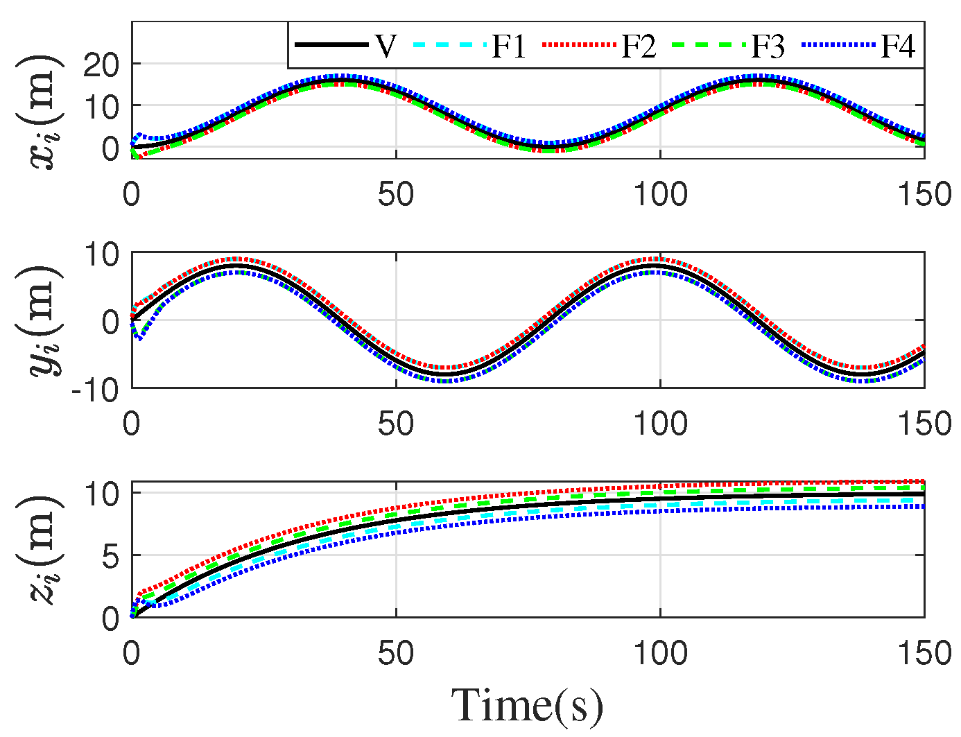
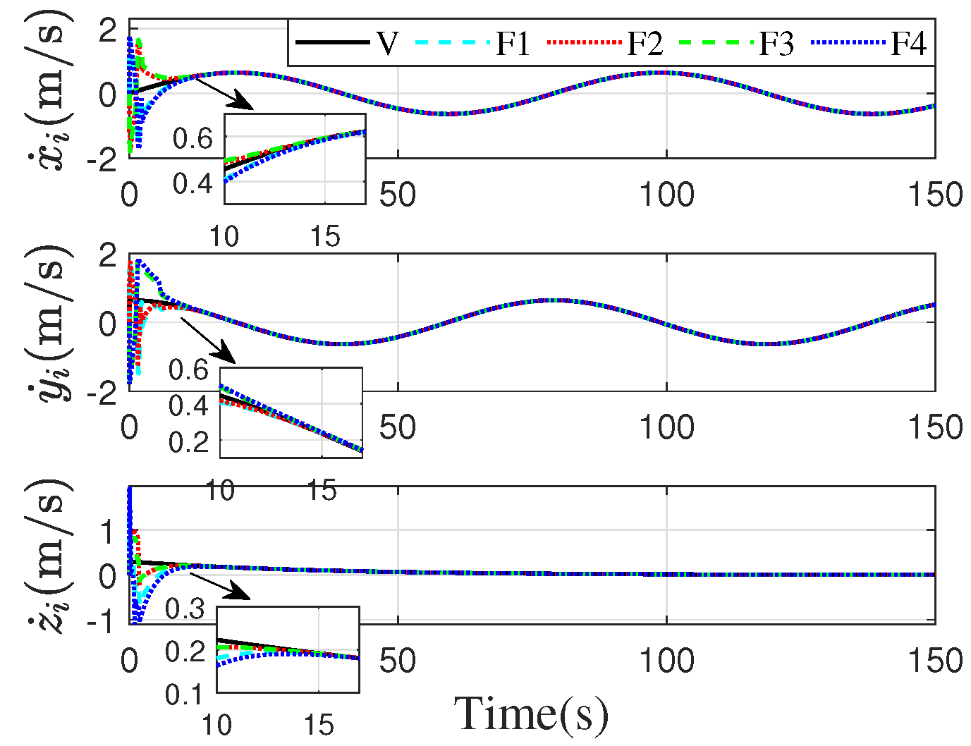
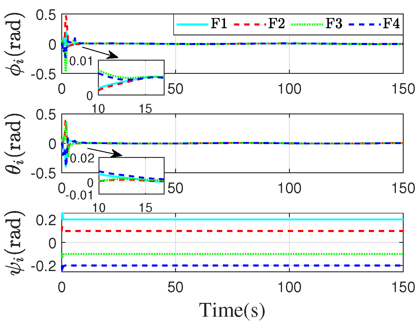
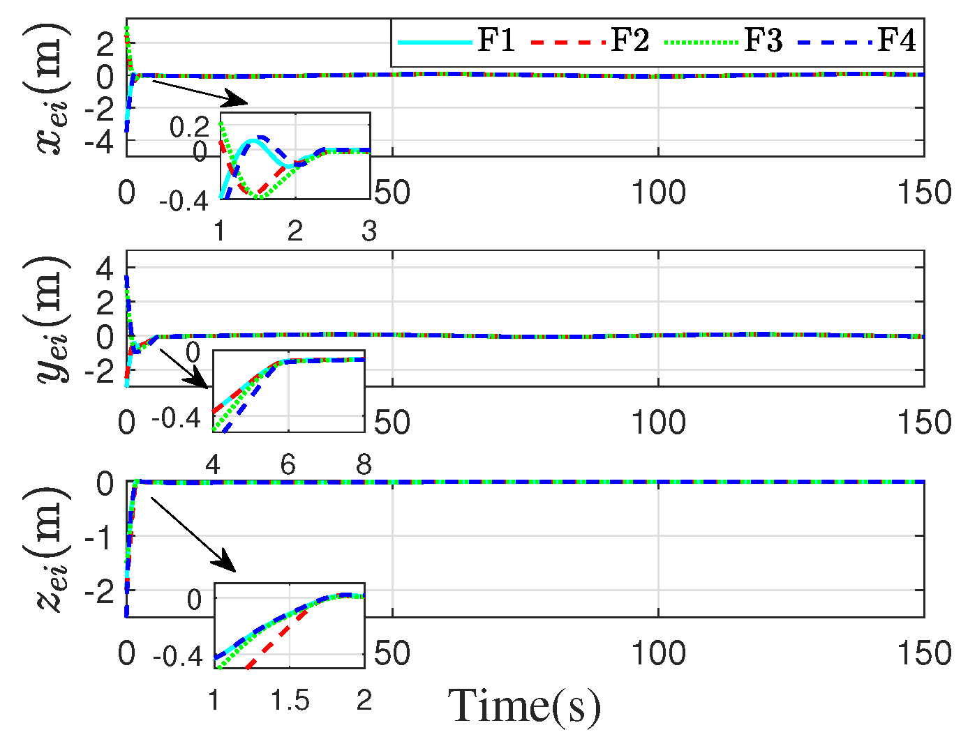
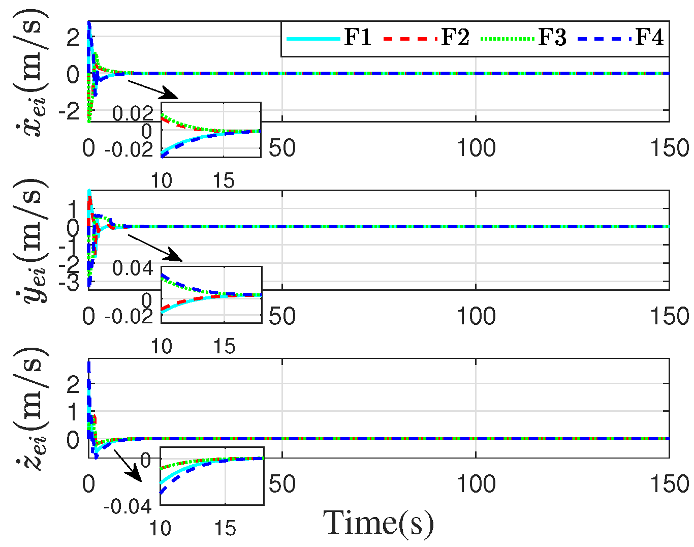
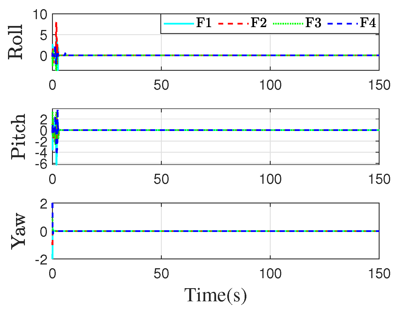
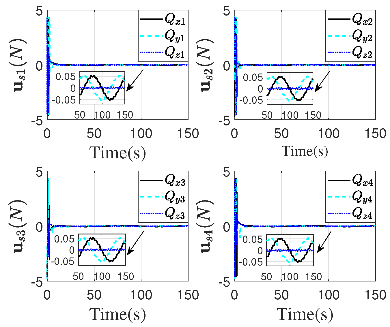
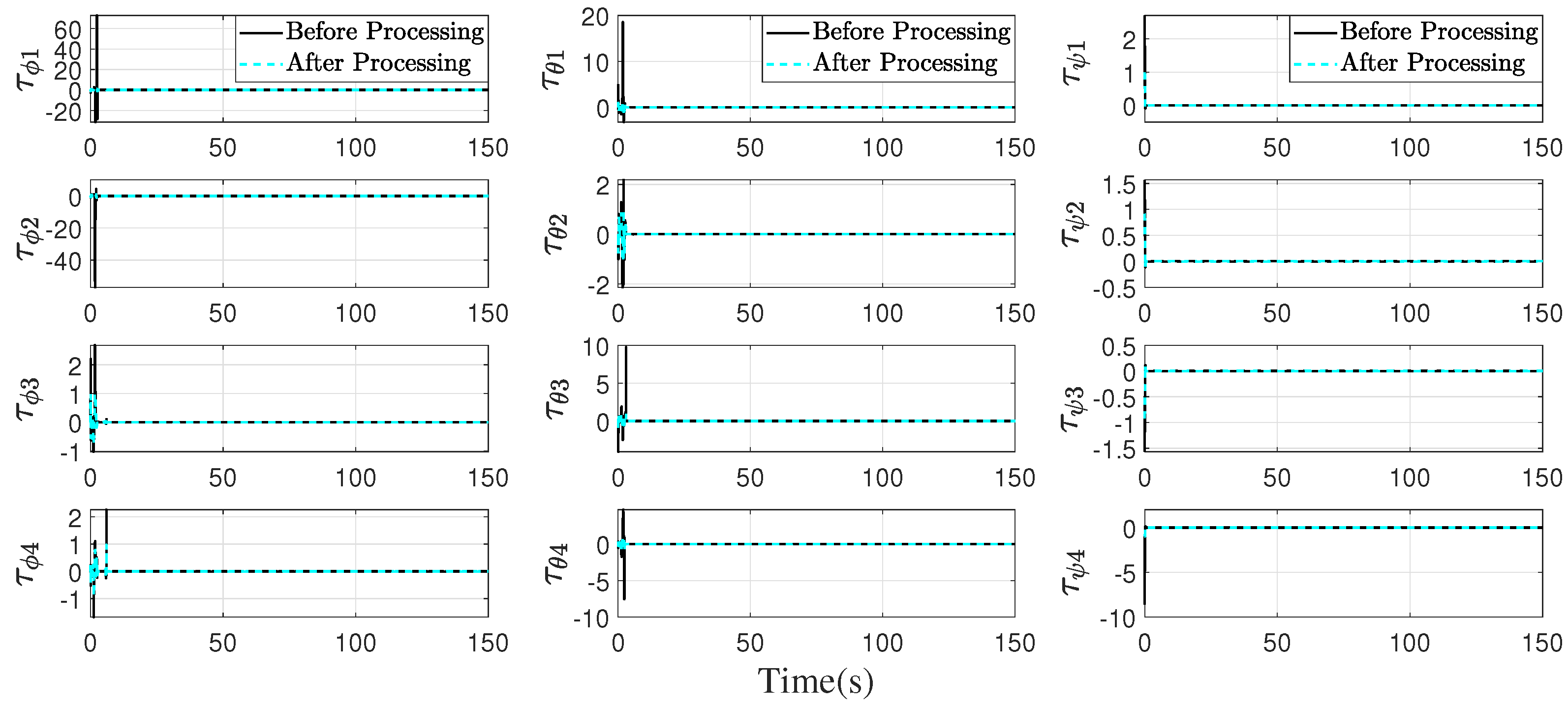
4.1. Simulation of the Proposed Method

The desired virtual leader trajectory P d in the three-dimensional space is established as P d ( t ) = 8 8 cos 2 t , 8 sin 2 t , 10 ( 1 e 0.3 t ) T . The unknown wind disturbances and other unmodeled dynamics of the translational dynamics and the rotational dynamics are set as d p 0 i = 0.1 sin ( t ) + 0.5 and d a 0 i = 0.1 sin ( t ) , respectively. Considering the safety distance between each UAV during actual flight, the initial position and attitude angle of follower UAVs are set as P 1 ( 0 ) = [ 0.5 , 0.5 , 0 ] T , P 2 ( 0 ) = [ 0.5 , 0.5 , 0 ] T , P 3 ( 0 ) = [ 0.5 , 0.5 , 0 ] T , P 4 ( 0 ) = [ 0.5 , 0.5 , 0 ] T , Θ 1 ( 0 ) = [ 0 , 0 , 0.2 ] T , Θ 2 ( 0 ) = [ 0 , 0 , 0.1 ] T , Θ 3 ( 0 ) = [ 0 , 0 , 0.1 ] T , Θ 4 ( 0 ) = [ 0 , 0 , 0.2 ] T . Table 2 shows the parameters of ESO, PTESO, and PTSMAC. Among them, c 1 c 4 denote critical controller parameters c 1 and c 3 serve as fundamental negative feedback parameters in prescribed-time sliding mode control, which are explicitly designed to ensure system stability—these parameters adopt larger values when initial errors are greater and smaller values otherwise. c 2 and c 4 represent gains of time-varying functions, indicating the weight of time-varying scaling functions in the overall negative feedback. They are typically set to 1.
The simulation results shown in Figure 4 and Figure 5 clearly demonstrate the complete process of the UAV formation transitioning from initial to terminal states. Firstly, the four follower UAVs rapidly converge to the prespecified initial formation distance Δ 0 i (i = 1, 2, 3, 4, unit: meter), where Δ 01 = [ 3.5 , 3.5 , 2 ] T , Δ 02 = [ 3 , 3 , 2 ] T , Δ 03 = [ 3.5 , 3.5 , 1.5 ] T , Δ 04 = [ 4 , 4 , 2.5 ] T . Immediately afterwards, while continuously tracking the trajectory of the virtual leader and always maintain the terminal formation distance Δ i (i = 1, 2, 3, 4, unit: meter) with the leader, where Δ 1 = [ 1 , 1 , 0.5 ] T , Δ 2 = [ 1 , 1 , 1 ] T , Δ 3 = [ 1 , 1 , 0.5 ] T , Δ 4 = [ 1 , 1 , 1 ] T . Throughout the formation process, each UAV maintains a safe distance that eliminates any risk of collision occurring. The symbols ∗ and ✩ in the figures denote the initial and final positions of the leader and follower UAVs, respectively.
Figure 6 and Figure 7 display the position tracking trajectories and velocity tracking trajectories of the follower UAVs, respectively. It can be observed that the follower UAVs accurately track the trajectory of the virtual leader V, and their velocity responses rapidly converge to the desired value. Figure 8 and Figure 9 respectively present the attitude angles and attitude angular velocity responses of the follower UAVs over time. Figure 8 shows that the attitude angles of follower UAVs converge to steady states quickly, demonstrating rapid dynamic response characteristics. Figure 9 illustrates that the attitude angular velocity converge rapidly, with the angular velocity responses of all attitude channels meeting the preset dynamic performance requirements.
Figure 10 and Figure 11 depict the position error and velocity error curves of the follower UAVs, respectively. It can be clearly seen that the position and velocity errors in the x, y, and z axes converge to 0 in a very short period. Figure 12 and Figure 13 show the attitude angle error and attitude angular velocity error curves of the follower UAVs, respectively. It can be seen from Figure 12 the attitude angle errors converge to 0 within the prescribed time T a = 6 s. Figure 13 shows that the attitude angular velocity errors converge to 0 within the prescribed time T a = 6 s.
Figure 14 shows the dynamic response curve of the sliding mode surface for follower UAVs. As can be seen from Figure 15, the intermediate control variables of the position loop strictly remain within the limitation range [−5, 5]. Figure 16 shows the control torque of the follower UAVs before and after saturation treatment. Evidently, the control torques after saturation processing all fall within the range of [−1, 1]. To more clearly illustrate the prescribed time convergence of the sliding mode surface and attitude angle errors within T a s = 3 s and T a = 6 s, an example of the error curves for a single UAV (F4) is presented, as shown in Figure 17 and Figure 18.

4.2. Simulation of Comparison with the Other Method

To validate the superiority of the proposed method, this subsection presents the simulation results obtained by using the distributed fixed-time control protocol (Equation (23)) proposed in [14].
The simulation results are shown in Figure 19, Figure 20, Figure 21 and Figure 22. According to the simulation results in Figure 19, Figure 20 and Figure 21, the position and velocity errors of the follower UAVs failed to converge to 0, and the roll and pitch angles continuously oscillated throughout the simulation. By contrast, the proposed method exhibits no sustained fluctuations under the same conditions, as shown in Figure 8. Figure 22 presents the simulation results of intermediate control variables in position loop without considering input constraints, clearly revealing that the input values are excessively large, even reach up to about 40 N.
Remark 3. 
If such a large initial input is applied during take-off, the UAV may lift off in a tilted attitude, causing it to deviate from the predefined trajectory at the initial stage of flight and potentially collide with the ground or surrounding objects. This scenario may lead to damage to onboard equipment and pose substantial safety risks. Therefore, it is evident that the proposed control method with input constraints is essential.
It can be clearly seen from the above simulation results that under the conditions where both speed and input are constrained, the proposed method enables the follower UAVs to accurately track the trajectory and speed of the virtual leader, achieving the desired formation configuration perfectly. Moreover, the attitude of the UAVs rapidly converges to a stable state. Meanwhile, it effectively ensures that the control inputs remain within the preset range, thus providing a reliable guarantee for the UAVs to safely achieve formation flight.

5. Conclusions

This study proposes a robust layered control strategy for networked quadrotor UAVs with inter-layer time-scale separation to achieve collaborative formation and prescribed-time attitude tracking under the constraints of UAV speed and control input. A distributed consensus protocol with input saturation constraints is adopted at the position loop layer to ensure formation stability and explicitly address speed constraints. At the attitude loop layer, a novel PTESO-based PTSMAC algorithm is proposed, which achieves specified-time convergence and effective interference compensation. Simulation results verify that the proposed method ensures attitude inner-loop state stability, strict input saturation compliance, and demonstrates better performance compared to traditional fixed-time methods. Future work will extend this framework to dynamic obstacle avoidance scenarios and heterogeneous UAV swarms with communication delays.

Author Contributions

Methodology, Z.W. (Zhikai Wang); Resources, F.T.; Writing—original draft, Y.Q.; Writing—review & editing, Z.W. (Zhihao Wu); Funding acquisition, S.G. All authors have read and agreed to the published version of the manuscript.

Funding

This paper is supported by the Scientific and Technological Project of Henan Province (Grant No. 242102221025, 252102220034), the Aeronautical Science Foundation of China (Grant No. 20240001042001), and the Key Scientific Research Projects of Universities in Henan Province (Grant No. 24B590001).

Data Availability Statement

The original contributions presented in this study are included in the article. Further inquiries can be directed to the corresponding author.

Conflicts of Interest

The authors declare no conflict of interest.

Appendix A

Proof of Theorem 1. 
The proof of this theorem is carried out in several steps: first, the boundedness of the control variable u x i is proved; next, v 2 x i is also proven to be bounded; then, the error state e x i is demonstrated to be fixed-time converge; and finally, it is shown that the distance error between distributed formation UAV and the virtual leading UAV converges to the desired range Δ x i .
Step 1: Prove the boundedness of the designed control input variable u x i .
According to Equation (21), when e x i < 0 , there is λ i σ e x i 0 , one can obtain that u x i = u max α i σ e x i / λ i + α i , yield α i u x i u max . Similarly, when e x i > 0 , there is 0 σ e x i λ i , it is clear that u x i = u max α i σ e x i / λ i α i , leading to u max u x i α i . Additionally, when e x i = 0 , it is obtained that u x i = 0 . In summary, it is always true that | u x i | u max .
Step 2: Prove the boundedness of the speed v 2 x i .
It is easy to obtain that | r x i |   m from Equation (19). Considering the boundary values of v 2 x i further, it follows that e x i = v 2 x i r x i v max m z i > 0 for v 2 x i = v max , which implies σ ( e x i ) = λ i and u x i = u max . Similarly, when v 2 x i = v max , this is e x i = v 2 x i r x i v max + m z i < 0 and σ ( e x i ) = λ i , yields u x i = u max . Then, one can obtain that
v ˙ 2 x i = b i u x i + e x d p i , if v 2 x i < v max b i u max + e x d p i , if v 2 x i = v max b i u max + e x d p i , if v 2 x i = v max
According to the Assumption 2, there is u max > e d max , which means that v ˙ 2 x i < 0 for v 2 x i = v max and v ˙ 2 x i > 0 for v 2 x i = v max . Where, e d max is the maximum disturbance estimate error. Besides, v 2 x i is a continuous and the initial value v 2 x i ( 0 ) in the given range v max , v max . Thus, it is easy to be concluded that | v 2 x i ( t ) | v max all the time.
Step 3: Prove the Fixed-time convergence of error state e x i .
Taking the time derivative of ζ i , yields
r ˙ x i = 2 k i ζ i 3 2 m k i 2 η i ζ i m 3 , if   2 m 3 k i η i < 4 m 3 k i k i ζ i , if   2 m 3 k i η i < 2 m 3 k i 2 k i ζ i + 3 2 m k i 2 η i ζ i + m 3 , if   4 m 3 k i η i < 2 m 3 k i
Here, due to | v 2 x i ( t ) | v max for t 0 , it can be inferred that | ζ i | 2 d i v max . Due to that k i < α i e d max / 2 d i v max in Equation (22), one can further obtain | r ˙ x i | α i e d max . Then, take the time derivative of e x i and substituting Equation (17) to it yields e ˙ x i = u x i + e x d p i r ˙ x i .
When e x i z i , according the designed controller Equation (21), it can be obtain that u x i = u max , which indicates e ˙ x i = u max + e x d p i r ˙ x i < u max α i < 0 . Similarly, when e x i z i , it is easy to deduce e ˙ x i = u max + e x d p i r ˙ x i > u max α i > 0 .
Besides, note that | v 2 x i ( 0 ) | v m a x , then e x i ( 0 ) v 2 x i ( 0 ) + r x i ( 0 ) v max + m . Thus, it is clear that within the given time T i 1 , the error e x i converges to the desired range bounded with z i , that is | e x i ( t ) | z i and σ e x i = e x i γ i for t T i 1 .
T i 1 ( v m a x + m z i ) / ( u m a x α i )
Furthermore, the dynamics of e x i is rewritten as
e ˙ x i = b i u max α i e x i γ i λ i b i α i sgn e x i + e x d p i r ˙ x i
Consequently, defining a Lyapunov candidate function as
V 1 i = 1 2 e x i 2
Then, considering the previous result | r ˙ x i |   α i e d max , and substituting Equation (A4) to the time derivative with the Lyapunov function yields
V ˙ 1 i = e x i u max α i e x i γ i λ i α i sgn e x i + e x d p i r ˙ x i u max α i λ i e x i γ i + 1 + ( e d max e x d p i ) e x i u max α i λ i 2 V 1 i γ i + 1 2 + δ τ i 2 V 1 i 1 2
where, δ τ i = e d max e x d p i > 0 . According to Lemma 3 and Equation (A6), one can obtain that the error e x i can converge to 0 within the fixed time T i p = T i 1 + T i 2 , the converge time unbounded is denoted as
T i 2 λ i 2 γ i 1 2 u max α i γ i 1 + 1 2 1 2 δ τ i
Step 4: Prove the consensus of state value x 1 i .
Then, the consensus of state variable system Equation (17) is considered. According to the assumption of the communication, the Laplace L is a non-singular M-matrix, there exists a diagonal matrix W = d i a g w 1 , w 2 , W N with w i > 0 , N is the number of the formation UAV, define G = W L + L T W is a positive matrix.
Considering V 2 = i = 1 N w i 0 η i r x i s d s , when t T , then one can obtain that V ˙ 2 = R ¯ T W L R ¯ = 1 2 R ¯ T G R ¯ λ min G 2 R ¯ 2 . Where R ¯ = r x 1 , r x 2 , , r x N T , λ min G is the minimum eigenvalue of G. According to Lyapunov stability theory, it can be concluded that lim t r x i η i t = 0 for all i = 1 , 2 , , N . Thus, one can obtain that lim t η i t = 0 , and lim t ( x 1 i x 1 j ) = 0 . That is to say, all the state value x 1 i converge to a same value.
This completes the proof. □

Appendix B

Proof of Theorem 2. 
To prove that the sliding surface S i converges to 0 within the prescribed time T a s , the following Lyapunov candidate function is selected:
V 3 i = 1 2 S i T S i
Differentiating both sides of Equation (A8) with respect to time yields
V ˙ 3 i = S i T S ˙ i = S i T x ˙ 4 i + h 4 x 4 i + c 3 p φ 2 ( T a s , T a ) x 3 i + h 4 φ ( T a s , T a ) x 4 i = S i T f Φ i + B ˜ Φ i Γ ˜ i + d q i + h 4 x 4 i + c 3 p φ 2 ( T a s , T a ) x 3 i + h 4 φ ( T a s , T a ) x 4 i = S i T d ^ Φ i c 3 + c 4 φ T d a , T a s S i η 2 s i g n S i c 3 + c 4 φ T d a , T a s V 3 i + S i T d ^ Φ i η 1 [   1   1   1   ] T
In the following, the proof will be continued over three time intervals.
(1)
when 0 t < T d a
T d a is the prescribed converge time for PTESO. Within this designated period, the system states have not yet attained the sliding mode surface, and estimation errors persist in the unknown disturbance vector d ^ Φ i , which are explicitly considered in the designed PTESO. Exponential convergence of the system is guaranteed if the maximum estimation errors fulfill the condition: Φ = S i T d ^ Φ i η 1 [   1   1   1   ] T < 0 . If this inequality does not hold, two alternative cases may occur.
Case 1: if c 3 + c 4 φ T d a , T a s V 3 i + Φ < 0 , one can obtain that V ˙ 3 i < 0 and the system will converge to 0.
Case 2: if c 3 + c 4 φ T d a , T a s V 3 i + Φ 0 , it can be obtained that max d ˜ q 1 i , d ˜ q 2 i > η 2 , then it can be obtained that V 3 i 1 / 2 Φ c 3 + c 4 φ T d a , T a s .
It can be obtained that when t approaches T d a , V 3 i converges to the bounded neighbourhood of a positive number.
(2)
when T d a t < T a s
In this time interval, the disturbance error can converge to 0 with the PTESO, which means d ˜ Φ i d ^ Φ i = 0 . Then, one can obtain that
V ˙ 3 i c 3 + c 4 φ T d a , T a s V 3 i
Then based on the Lemma 1, obtaining that S i converge to 0 at the prescribed time T a s .
(3)
when t T a s
In this time interval, it is clear that V ˙ 3 i c 3 + c 4 p T a s T d a V 3 i 0 . According to the Lyapunov stability theory, it can obtain 0 V 3 i t V 3 i T a s ; that is, S i 0 t T a s . To analyze the motion of the system state after reaching the sliding surface, the following Lyapunov function is selected:
V 4 i = 1 2 x 3 i T x 3 i
Due to S i = 0 when t > T a s ; combining Equation (31) the following equation can be obtained:
x 4 i = c 1 + c 2 φ T a s , T a x 3 i
Submitting Equation (A12) to Equation (A11) can obtain
V ˙ 4 i = x 3 i x ˙ 3 i = x 3 i T x 4 i = c 1 + c 2 φ T a s , T a x 3 i T x 3 i = 2 c 1 + c 2 φ T a s , T a V 4 i
According to Lemma 1, it can be obtained that x 3 i can converge to 0 at the prescribed time T a s . When t T a s , V ˙ 4 i 2 h 3 + h 4 p T a T a s V 4 i 0 as well as 0 V 4 i t V 4 i T a ; that is, x 3 i 0 t T a s . In addition, according to the definition of the sliding surface, if S i 0 , x 3 i 0 satisfy, x 4 i 0 holds.
This completes the proof. □

References

  1. Huang, J.; Luo, Y.; Quan, Q.; Wang, B.; Xue, X.; Zhang, Y. An autonomous task assignment and decision-making method for coverage path planning of multiple pesticide spraying UAVs. Comput. Electron. Agric. 2023, 212, 108128. [Google Scholar] [CrossRef]
  2. Muñoz, F.; Zúñiga-Peña, N.S.; Carrillo, L.R.G.; Espinoza, E.S.; Salazar, S.; Márquez, M.A. Adaptive fuzzy consensus control strategy for UAS-based load transportation tasks. IEEE Trans. Aerosp. Electron. Syst. 2021, 57, 3844–3860. [Google Scholar] [CrossRef]
  3. Lu, L.; Dai, F. Accurate road user localization in aerial images captured by unmanned aerial vehicles. Autom. Constr. 2024, 158, 105257. [Google Scholar] [CrossRef]
  4. Fan, J.; Lei, L.; Cai, S.; Shen, G.; Cao, P.; Zhang, L. Area surveillance with low detection probability using UAV swarms. IEEE Trans. Veh. Technol. 2023, 73, 1736–1752. [Google Scholar] [CrossRef]
  5. Zhang, C.; Guo, J.; Wang, F.; Chen, B.; Fan, C.; Yu, L.; Wang, Z. A dynamic parameters genetic algorithm for collaborative strike task allocation of unmanned aerial vehicle clusters towards heterogeneous targets. Appl. Soft Comput. 2025, 175, 113075. [Google Scholar] [CrossRef]
  6. Xu, L.X.; Wang, Y.L.; Wang, X.; Peng, C. Distributed active disturbance rejection formation tracking control for quadrotor UAVs. IEEE Trans. Cybern. 2023, 54, 4678–4689. [Google Scholar] [CrossRef]
  7. Meng, R.; Chen, S.; Hua, C.; Qian, J.; Sun, J. Disturbance observer-based output feedback control for uncertain QUAVs with input saturation. Neurocomputing 2020, 413, 96–106. [Google Scholar] [CrossRef]
  8. Yu, Y.; Guo, J.; Ahn, C.K.; Xiang, Z. Neural adaptive distributed formation control of nonlinear multi-UAVs with unmodeled dynamics. IEEE Trans. Neural Netw. Learn. Syst. 2022, 34, 9555–9561. [Google Scholar] [CrossRef]
  9. Zou, Y.; Xia, K.; He, W. Adaptive fault-tolerant distributed formation control of clustered vertical takeoff and landing UAVs. IEEE Trans. Aerosp. Electron. Syst. 2021, 58, 1069–1082. [Google Scholar] [CrossRef]
  10. Zheng, L.; Deng, F.; Yu, Z.; Luo, Y.; Zhang, Z. Multilayer neural dynamics-based adaptive control of multirotor UAVs for tracking time-varying tasks. IEEE Trans. Syst. Man, Cybern. Syst. 2021, 52, 5889–5900. [Google Scholar] [CrossRef]
  11. Xiong, H.; Zhang, Y. Reinforcement learning-based formation-surrounding control for multiple quadrotor UAVs pursuit-evasion games. ISA Trans. 2024, 145, 205–224. [Google Scholar] [CrossRef] [PubMed]
  12. Jia, J.; Chen, X.; Wang, W.; Wu, K.; Xie, M. Distributed observer-based finite-time control of moving target tracking for UAV formation. ISA Trans. 2023, 140, 1–17. [Google Scholar] [CrossRef]
  13. Yu, D.; Ma, S.; Liu, Y.J.; Wang, Z.; Chen, C.P. Finite-time adaptive fuzzy backstepping control for quadrotor UAV with stochastic disturbance. IEEE Trans. Autom. Sci. Eng. 2023, 21, 1335–1345. [Google Scholar] [CrossRef]
  14. Su, Y.H.; Bhowmick, P.; Lanzon, A. A fixed-time formation-containment control scheme for multi-agent systems with motion planning: Applications to quadcopter UAVs. IEEE Trans. Veh. Technol. 2024, 73, 9495–9507. [Google Scholar] [CrossRef]
  15. Miao, Q.; Zhang, K.; Jiang, B. Fixed-time collision-free fault-tolerant formation control of multi-UAVs under actuator faults. IEEE Trans. Cybern. 2024, 54, 3679–3691. [Google Scholar] [CrossRef] [PubMed]
  16. Tan, M.; Shen, H. Three-dimensional cooperative game guidance law for a leader–follower system with impact angles constraint. IEEE Trans. Aerosp. Electron. Syst. 2023, 60, 405–420. [Google Scholar] [CrossRef]
  17. Gong, W.; Li, B.; Ahn, C.K.; Yang, Y. Prescribed-time extended state observer and prescribed performance control of quadrotor UAVs against actuator faults. Aerosp. Sci. Technol. 2023, 138, 108322. [Google Scholar] [CrossRef]
  18. Tian, M.; Wang, N.; Wang, Z.; Fu, Z.; Tao, F. Prescribed-time fault-tolerant tracking control for quadrotor UAV with guaranteed performance. Aerosp. Sci. Technol. 2025, 161, 110162. [Google Scholar] [CrossRef]
  19. Shao, X.; Sun, G.; Yao, W.; Liu, J.; Wu, L. Adaptive sliding mode control for quadrotor UAVs with input saturation. IEEE/ASME Trans. Mechatronics 2021, 27, 1498–1509. [Google Scholar] [CrossRef]
  20. Wang, C.; Li, W.; Liang, M. Event-triggered finite-time adaptive neural network control for quadrotor UAV with input saturation and tracking error constraints. Aerosp. Sci. Technol. 2024, 155, 109658. [Google Scholar] [CrossRef]
  21. Mofid, O.; Mobayen, S. Adaptive finite-time backstepping global sliding mode tracker of quad-rotor UAVs under model uncertainty, wind perturbation, and input saturation. IEEE Trans. Aerosp. Electron. Syst. 2021, 58, 140–151. [Google Scholar] [CrossRef]
  22. Wang, Q.; Wang, W.; Suzuki, S. UAV trajectory tracking under wind disturbance based on novel antidisturbance sliding mode control. Aerosp. Sci. Technol. 2024, 149, 109138. [Google Scholar] [CrossRef]
  23. Xing, Z.; Zhang, Y.; Su, C.Y. Active wind rejection control for a quadrotor UAV against unknown winds. IEEE Trans. Aerosp. Electron. Syst. 2023, 59, 8956–8968. [Google Scholar] [CrossRef]
  24. Wang, G.; Zuo, Z.; Wang, C. Robust consensus control of second-order uncertain multiagent systems with velocity and input constraints. Automatica 2023, 157, 111226. [Google Scholar] [CrossRef]
  25. Geng, M.J.; Ding, H.F.; Yao, X.Y.; Liu, W.J.; Hua, M. Noncooperative Game of Distributed Quadrotor UAVs With Multiple Constraints. IEEE Trans. Aerosp. Electron. Syst. 2024, 60, 4728–4739. [Google Scholar] [CrossRef]
  26. Teng, L.; Chuanjiang, L.; Yanning, G.; Guangfu, M. Three-dimensional finite-time cooperative guidance for multiple missiles without radial velocity measurements. Chin. J. Aeronaut. 2019, 32, 1294–1304. [Google Scholar]
  27. Ren, Y.H.; Zhou, W.N.; Li, Z.W.; Liu, L.; Sun, Y.Q. Prescribed-time cluster lag consensus control for second-order non-linear leader-following multiagent systems. ISA Trans. 2021, 109, 49–60. [Google Scholar] [CrossRef] [PubMed]
  28. Cui, L.; Jin, N. Prescribed-time ESO-based prescribed-time control and its application to partial IGC design. Nonlinear Dyn. 2021, 106, 491–508. [Google Scholar] [CrossRef]
  29. Xu, Y.; Qu, Y.; Luo, D.; Duan, H. Distributed fixed-time time-varying formation-containment control for networked underactuated quadrotor UAVs with unknown disturbances. Aerosp. Sci. Technol. 2022, 130, 107909. [Google Scholar] [CrossRef]
  30. Wang, Z.; Fang, Y.; Fu, W.; Ma, W.; Wang, M. Prescribed-time cooperative guidance law against manoeuvring target with input saturation. Int. J. Control 2023, 96, 1177–1189. [Google Scholar] [CrossRef]
  31. Chen, M.; Tao, G.; Jiang, B. Dynamic surface control using neural networks for a class of uncertain nonlinear systems with input saturation. IEEE Trans. Neural Netw. Learn. Syst. 2014, 26, 2086–2097. [Google Scholar] [CrossRef] [PubMed]
Figure 1. System structure diagram of quadrotor UAV.
Drones 09 00417 g001
Figure 2. Distributed formation and tracking controller framework for multiple networked UAVs.
Drones 09 00417 g002
Figure 3. Communication topology of the multi-UAV system.
Drones 09 00417 g003
Figure 4. The three-dimensional position trajectories of the leader and follower UAVs.
Drones 09 00417 g004
Figure 5. The top view of the position trajectories of the leader and follower UAVs.
Drones 09 00417 g005
Figure 6. The two-dimensional position trajectories of the leader and follower UAVs.
Drones 09 00417 g006
Figure 7. The speed of the leader and follower UAVs.
Drones 09 00417 g007
Figure 8. The attitude angle of the follower UAVs.
Drones 09 00417 g008
Figure 9. The attitude angular velocity of the follower UAVs.
Drones 09 00417 g009
Figure 10. The position error of the follower UAVs.
Drones 09 00417 g010
Figure 11. The velocity error of the follower UAVs.
Drones 09 00417 g011
Figure 12. The attitude angle error of the follower UAVs.
Drones 09 00417 g012
Figure 13. The attitude angular velocity error of the follower UAVs.
Drones 09 00417 g013
Figure 14. The sliding mode surface of the follower UAVs.
Drones 09 00417 g014
Figure 15. The intermediate control variables of the follower UAVs in the position loop.
Drones 09 00417 g015
Figure 16. The control torque of the follower UAVs before and after saturation processing.
Drones 09 00417 g016
Figure 17. The sliding mode surface of F4.
Drones 09 00417 g017
Figure 18. The attitude angle error of F4.
Drones 09 00417 g018
Figure 19. The position error of the follower UAVs.
Drones 09 00417 g019
Figure 20. The velocity error of the follower UAVs.
Drones 09 00417 g020
Figure 21. The attitude angle of the follower UAVs.
Drones 09 00417 g021
Figure 22. The intermediate control variables of the follower UAVs in the position loop.
Drones 09 00417 g022
Table 1. Quadrotor UAVs parameters.
ParameterValuesUnit
m0.5kg
g9.8m/s2
l0.225m
c T 1.681 × 10 5 N/(rad/s)2
c M 2.783 × 10 7 N·m/(rad/s)2
I x 2.276 × 10 2 kg·m2
I y 2.276 × 10 2 kg·m2
I z 3.132 × 10 2 kg·m2
I r 6.16 × 10 5 kg·m2
K p i diag ( 0.1 , 0.1 , 0.1 ) N·s/rad
K a i diag ( 0.1 , 0.1 , 0.1 ) N·s/rad
Table 2. Controller parameters.
Parameter CategorySymbolValue
ESO parameters γ 1 200
γ 2 300
μ 1 0.5
δ 1 0.1
PTESO parameters k 1 3.82
k 2 6.94
k 3 1.5
Γ 1.2
ζ 0.6
t ¯ f 0
T d a 0
PTSMAC parameters c 1 4
c 2 1
c 3 6
c 4 1
η 1 5
T a s 3
T a 6
Disclaimer/Publisher’s Note: The statements, opinions and data contained in all publications are solely those of the individual author(s) and contributor(s) and not of MDPI and/or the editor(s). MDPI and/or the editor(s) disclaim responsibility for any injury to people or property resulting from any ideas, methods, instructions or products referred to in the content.

