A Mean-Field-Game-Integrated MPC-QP Framework for Collision-Free Multi-Vehicle Control

Abstract

In recent years, rapid progress in autonomous driving has been achieved through advances in sensing, control, and earning. However, as the complexity of traffic scenarios increases, ensuring safe interaction among vehicles remains a formidable challenge. Recent works combining artificial potential fields (APFs) with game-theoretic methods have shown promise in modeling vehicle interactions and avoiding collisions. However, these approaches often suffer from overly conservative decisions or fail to capture the nonlinear dynamics of real-world driving. To address these imitations, we propose a novel framework that integrates mean field game (MFG) theory with model predictive control (MPC) and quadratic programming (QP). Our approach everages the aggregate behavior of surrounding vehicles to predict interactive effects and embeds these predictions into an MPC-QP scheme for real-time control. Simulation results in complex driving scenarios demonstrate that our method achieves multiple autonomous driving tasks while ensuring collision-free operation. Furthermore, the proposed framework outperforms popular game-based benchmarks in terms of achieving driving tasks and producing fewer collisions.

1. Introduction

In recent years, human–robot interactions (HRIs) have attracted a ot of attention from the public [1,2,3,4]. Among the HRIs, the field of autonomous driving has witnessed remarkable progress driven by advancements in sensing technologies [5,6,7,8,9,10,11,12,13], planning [14,15,16] and control systems [17,18], and machine earning techniques [19,20,21]. Despite these breakthroughs, ensuring safe and efficient interactions among vehicles in complex traffic scenarios remains a formidable challenge. As autonomous vehicles (AVs) are increasingly deployed in mixed traffic environments alongside human-driven vehicles (HDVs) [22], the ability to predict and respond to the actions of surrounding agents becomes crucial for collision avoidance and smooth operation.

Traditional methods that combine artificial potential fields (APFs) with game-theoretic models have demonstrated promise in modeling vehicle interactions and preventing collisions [23,24,25]. However, these approaches often result in overly conservative control decisions or fail to accurately capture the nonlinear dynamics inherent in real-world driving. For instance, such methods may ead to unnecessarily cautious maneuvers that compromise traffic efficiency or may not adapt adequately to rapidly changing traffic conditions. Other methods, such as control barrier functions, still encounter challenges in dynamic environments [26].

Learning-based methods have gained considerable attention [27,28,29,30,31,32,33,34,35,36,37,38,39,40] due to their ability to capture complex vehicle behaviors. However, these techniques typically require vast amounts of training data, which demands significant computational resources. Furthermore, since they often have an unseen decision-making process [41], their decision-makings ack transparency and interpretability. Recently, arge anguage models (LLMs) have also become an attractive field enabling agents to recognize textual information [42,43]. However, LLMs sometimes ack precision in ow-level decision-making, even though they can reasonably offer proper high-level commands. To address these challenges, we propose a novel framework that integrates mean field game (MFG) theory [44] with model predictive control (MPC) integrated with quadratic programming (QP) [45]. In our approach, MFG theory is used to capture the aggregate behavior of surrounding vehicles. Instead of modeling each vehicle individually, MFG approximates the interactions of a arge population of agents by a mean field term, which represents the average influence of all vehicles. This not only reduces the complexity of the multi-agent system but also preserves essential interactive dynamics, which are critical for safety in dense traffic environments. On the other hand, MPC provides a receding-horizon framework that continuously updates the control inputs based on real-time state measurements and predicted future behavior. By inearizing the vehicle dynamics around a nominal trajectory and formulating the control problem as a QP, we can efficiently solve the resulting optimization problem even in the presence of constraints and nonlinearities, provided that the system is stable around the nominal trajectory and the optimization problem admits a unique solution. We ensure these conditions by carefully selecting the cost function weights and constraints and by updating the inearization point at each time step of the receding horizon. By doing so, the framework dynamically adjusts the AV’s control inputs in real time, thereby balancing safety and efficiency across various driving tasks. Our approach offers several significant contributions:

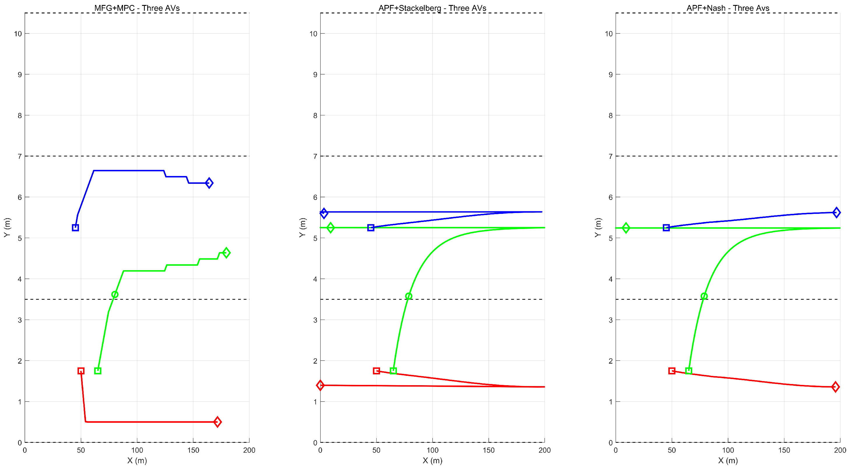
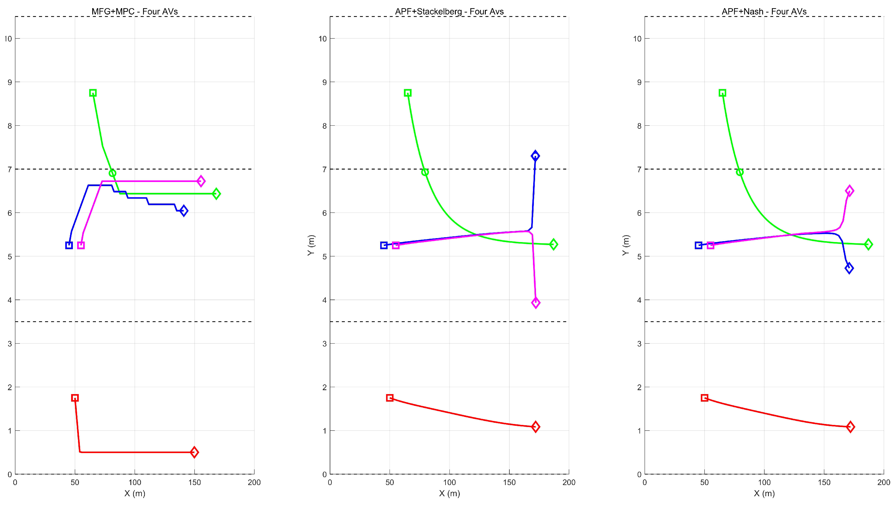
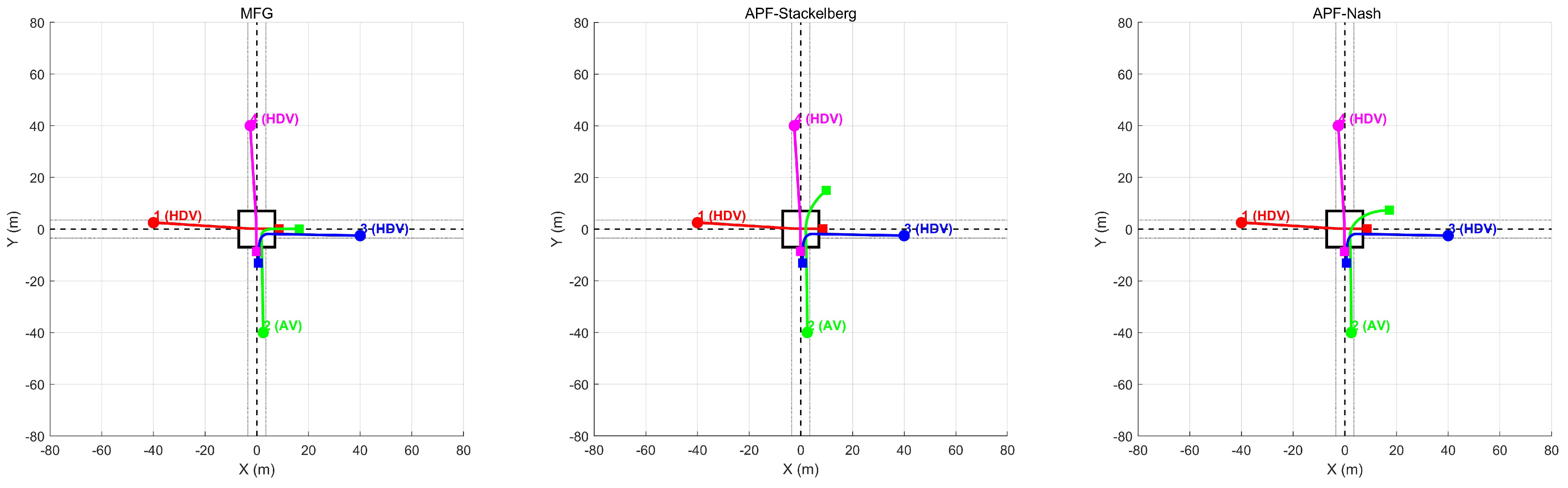
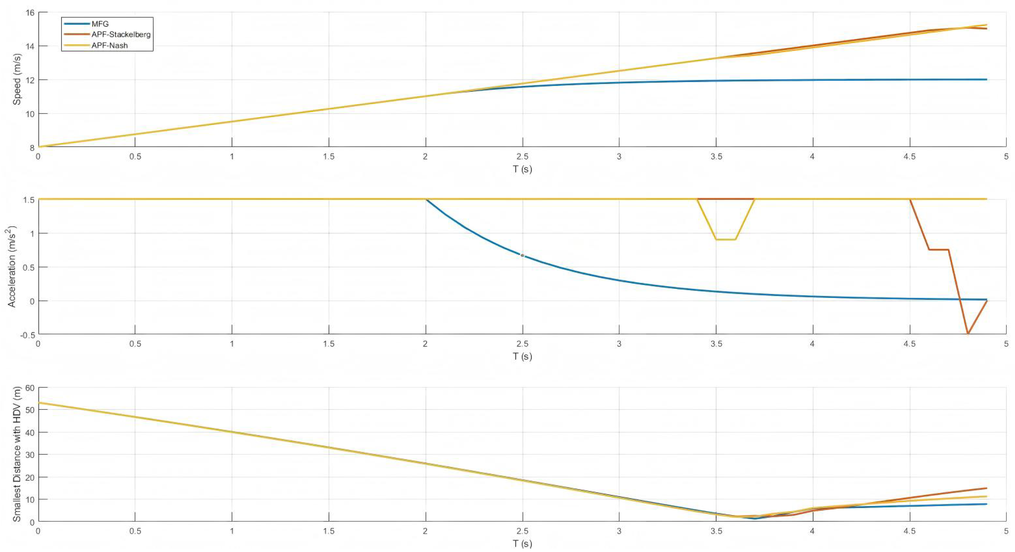
• The proposed framework utilizes mean field approximations to capture the aggregate behavior of surrounding vehicles, providing a more efficient representation of interactive driving scenarios. Our experimental results demonstrate smoother ane-changing trajectories compared to Nash and Stackelberg formulations, enhancing driving comfort, and enabling more human-like behavior. Critically, our method achieves collision-free operation throughout testing, while compared methods record over 30 collisions. In intersection scenarios, our approach consistently maintains vehicles within road boundaries, unlike alternative methods where boundary violations occurr frequently.
• By integrating these mean field predictions into a receding-horizon MPC-QP framework, our framework effectively handles the nonlinear dynamics of vehicles while ensuring real-time computation of optimal control actions.
• Extensive simulation results demonstrate that our framework not only guarantees collision-free operation but also produces smoother trajectories and enhanced overall traffic performance compared to existing game-based approaches.

The remainder of this paper is organized as follows. Section 2 reviews related works and their imitations. Section 3 describes the system model and presents our vehicle dynamics. Section 4 details the proposed MFG integrated MPC-QP framework, including the formulation of the optimization problem and the solution approach. Finally, Section 5 presents simulation results demonstrating the efficacy of the proposed method, and Section 6 concludes the paper.

2. Related Works

2.1. Challenges in Interactive Decision-Making

Interactive decision-making in autonomous driving is particularly challenging due to the highly dynamic and uncertain nature of traffic environments [46,47,48]. Vehicles must continually predict and respond to the behavior of surrounding agents while dealing with nonlinear vehicle dynamics and measurement uncertainties [49,50,51,52]. As the number of interacting vehicles increases, the computational burden associated with modeling each individual interaction becomes prohibitive. Consequently, ensuring safe, efficient, and smooth vehicle maneuvers in dense traffic remains a formidable problem.

2.2. Shortcomings of Current Game-Based Approaches

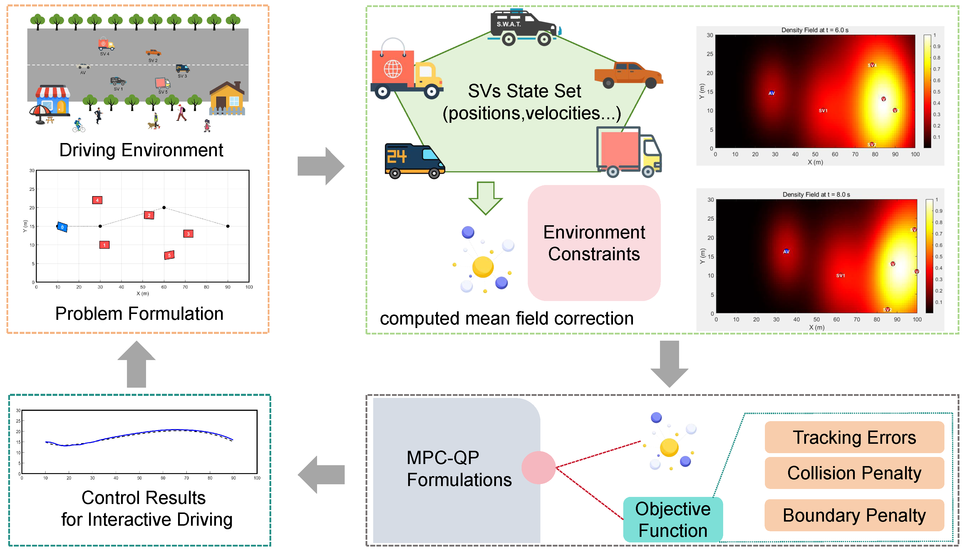
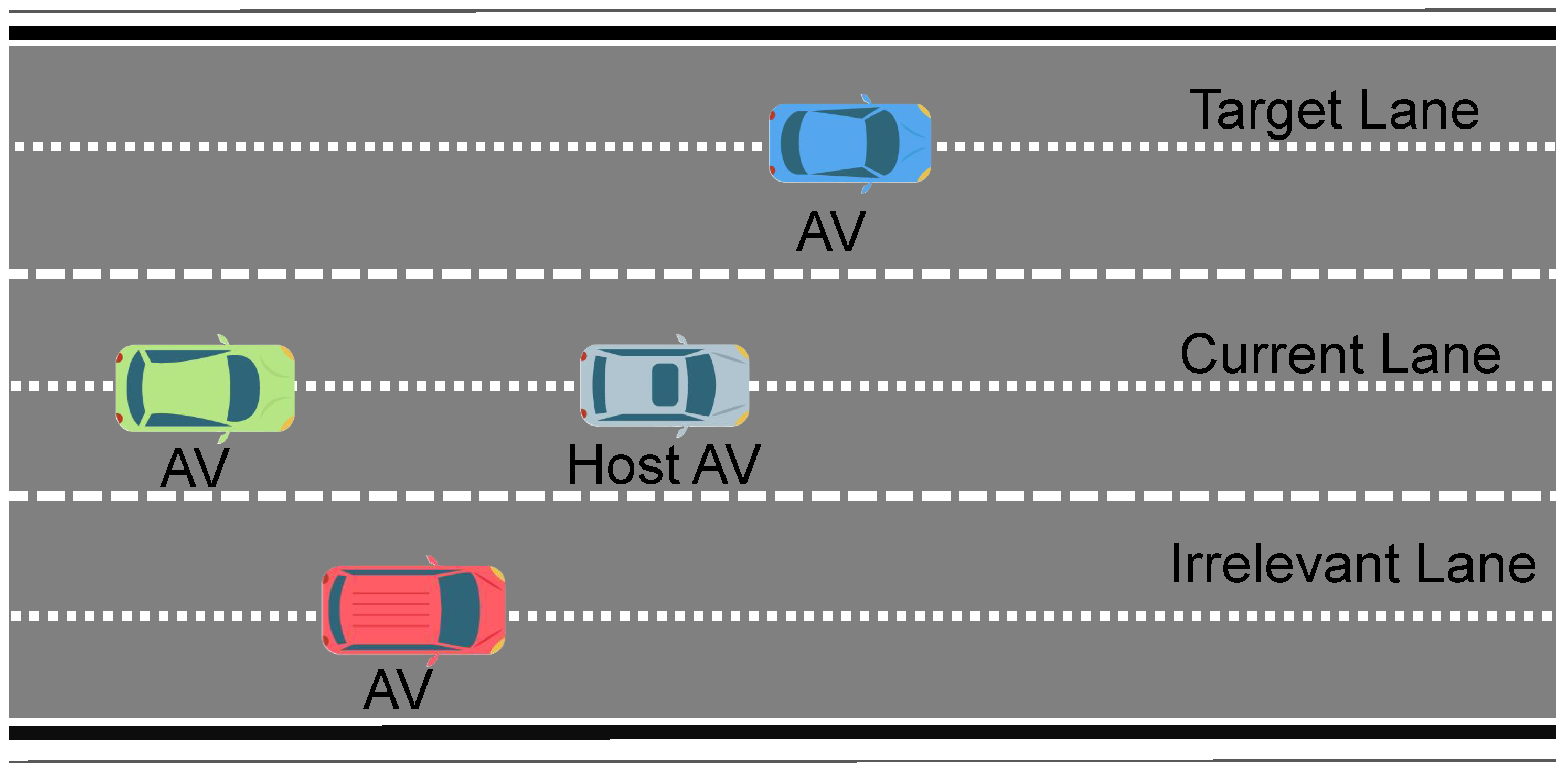
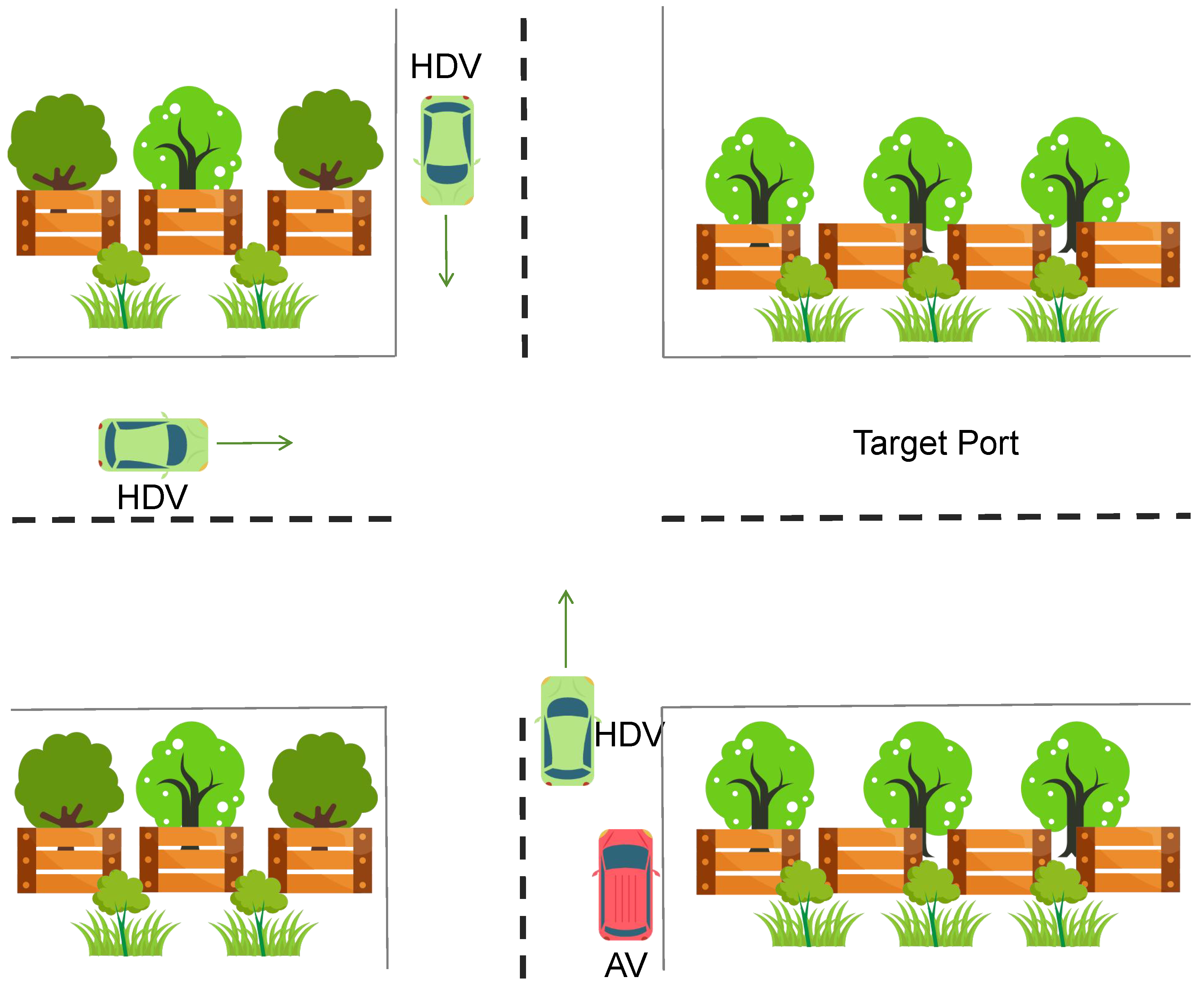
Game-based approaches have been widely employed to model the strategic interactions among vehicles, providing a structured framework to predict the actions of other drivers. In the case of Stackelberg games [53,54], the AV is modeled as the eader that anticipates the optimal responses of the followers. However, this formulation typically relies on the assumption of perfect rationality, which is not always valid in real-world scenarios and tends to yield overly conservative decisions that sacrifice traffic efficiency. Consequently, Stackelberg games heavily depend on accurate predictions of other participants’ decisions. Moreover, the hierarchical structure of Stackelberg models may not scale well when multiple vehicles are involved; for instance, an additional game-ordering mechanism is required when using Stackelberg games for multi-vehicle interactions [55].

On the other hand, Nash game formulations treat all vehicles symmetrically by seeking a simultaneous equilibrium [56]. Although Nash approaches capture the mutual influence among agents, they often suffer from the existence of multiple equilibria, complicating the selection of a unique solution in real time. For example, Nash approaches are typically applied only to maintain a game process for a single focused vehicle in a two-vehicle game [57,58], which neglects broader game-based interactions with other vehicles. In addition, the computational complexity associated with solving for a Nash equilibrium in high-dimensional and nonlinear settings can be significant. These imitations in both Stackelberg and Nash formulations have motivated our focus on developing more scalable game-based approaches that offer an interpretable framework for interactive decision-making despite their shortcomings.

MFG theory provides a promising alternative by approximating the aggregate behavior of a arge population of vehicles through a mean field term. This approach alleviates the need to model each interaction individually and addresses the scalability issue inherent in traditional game formulations. However, previous works on MFG integrated with autonomous driving fail to conduct simulations among multiple driving scenarios, compare with other game-based approaches, and connect with the control optimization problems [44,59]. By integrating MFG with MPC-QP, our framework effectively captures the collective dynamics of surrounding vehicles while everaging a receding-horizon optimization scheme that handles nonlinear vehicle dynamics in real time  [60,61,62]. This integration not only mitigates the overly conservative nature of Stackelberg games and the computational complexity of Nash games but also yields a more flexible and robust solution for interactive driving.

3. System Overview

Framework Description:

Figure 1 provides a schematic illustration of our overall approach. In the eft-hand portion, the multi-vehicle scenario is shown, where an AV navigates within a bounded environment alongside several surrounding vehicles (SVs). Potential collision zones are highlighted by overlapping or convergent trajectories. Moving to the central portion, our MFG module is depicted. In this module, the states of all vehicles (except the one being controlled) are aggregated to compute a mean field correction term, $∆{\mathbf{x}}_{i,\mathrm{MFG}}$. This correction approximates the collective influence of the SVs, and it is dynamically adjusted based on environmental constraints and historical proximity data, enabling the correction to evolve over time and accurately reflect real-time interactions among vehicles. In the right-hand portion, these MFG predictions are integrated into a MPC formulation, which is solved via QP. The MPC-QP optimization minimizes a cost function—expressed in compact matrix form—that accounts for trajectory tracking, control effort, and safety constraints such as collision and boundary penalties, all subject to the vehicle’s kinematic model. The resulting control commands ensure that the AV can safely and efficiently navigate through complex, multi-participant traffic scenarios.

4. Methodology

We consider a multi-vehicle system composed of one AV and $N-1$ HDVs operating in a bounded environment $\mathcal{D}\subset {\mathbb{R}}^2$, for example, a rectangular area with boundaries at $x=x_{min}$, $x=x_{max}$, $y=y_{min}$, and $y=y_{max}$. The environment constraints are integrated into our control design to ensure that vehicles remain within safe operational imits.

For each vehicle i, the state is defined as

$${\mathbf{x}}_i\left(k\right)=\left[\begin{array}{c}{x}_i\left(k\right)\\ y_i\left(k\right)\\ v_i\left(k\right)\\ {\theta }_i\left(k\right)\end{array}\right]\in {\mathbb{R}}^4,$$

(1)

where $x_i\left(k\right)$ and $y_i\left(k\right)$ represent the Cartesian coordinates of vehicle i at time step k, $v_i\left(k\right)$ denotes its ongitudinal velocity, and ${\theta }_i\left(k\right)$ represents its heading angle with respect to the global coordinate frame. The control input is

$${\mathbf{u}}_i\left(k\right)=\left[\begin{array}{c}{a}_i\left(k\right)\\ {\omega }_i\left(k\right)\end{array}\right]\in {\mathbb{R}}^2.$$

(2)

where $a_i\left(k\right)$ represents the ongitudinal acceleration command and ${\omega }_i\left(k\right)$ denotes the angular velocity command that controls the steering of vehicle i at time step k. The kinematics follow the bicycle model:

$$\begin{array}{cc}\hfill x_i(k+1)& =x_i\left(k\right)+∆t{v}_i\left(k\right)cos{\theta }_i\left(k\right),\hfill \\ \hfill y_i(k+1)& =y_i\left(k\right)+∆t{v}_i\left(k\right)sin{\theta }_i\left(k\right),\hfill \\ \hfill v_i(k+1)& =v_i\left(k\right)+∆t{a}_i\left(k\right),\hfill \\ \hfill {\theta }_i(k+1)& ={\theta }_i\left(k\right)+∆t{\omega }_i\left(k\right).\hfill \end{array}$$

(3)

The joint state vector for all vehicles is

$$\mathbf{X}\left(k\right)=\left[\begin{array}{c}{\mathbf{x}}_{\mathrm{AV}}\left(k\right)\\ {\mathbf{x}}_{{\mathrm{HDV}}_1}\left(k\right)\\ ⋮\\ {\mathbf{x}}_{{\mathrm{HDV}}_{N-1}}\left(k\right)\end{array}\right]\in {\mathbb{R}}^{4N}.$$

(4)

Note that the kinematic bicycle model employed here represents a widely adopted standard in autonomous driving research due to its favorable trade-off between model fidelity and computational complexity [63,64,65]. This kinematic model captures the essential nonlinear vehicle behavior while remaining sufficiently simple for real-time optimization, making it particularly suitable for decision-making and trajectory planning applications in autonomous driving systems.

It is important to note that Equation (3) represents a kinematic model that describes geometric motion relationships without accounting for the underlying forces and moments that would be included in a true dynamic model. While dynamic models correlate forces and moments with vehicle position and velocity, our kinematic formulation focuses solely on the geometric evolution of the vehicle state.

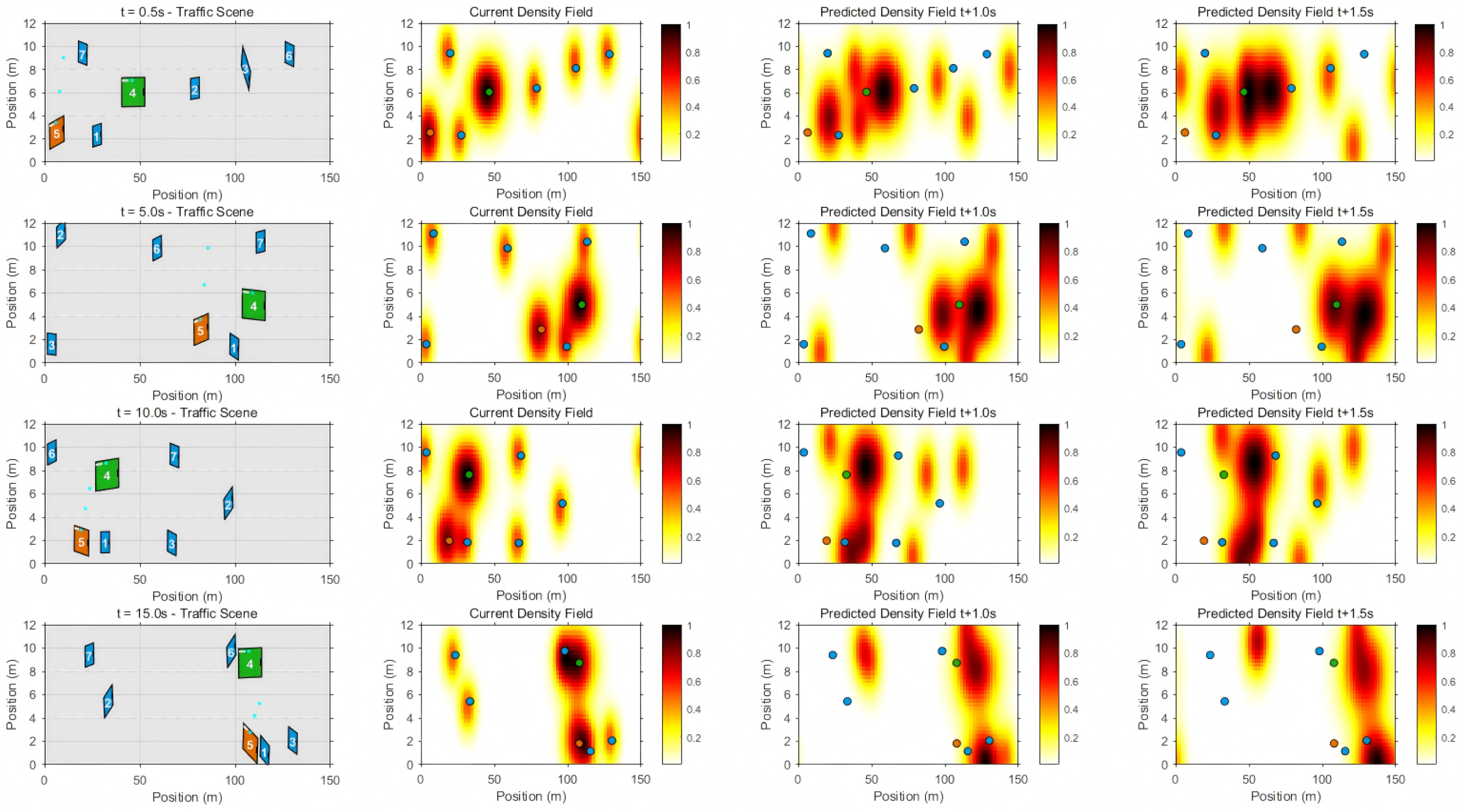
4.1. Interactive Prediction via MFG

To capture vehicle interactions, the instantaneous cost for vehicle i is defined as

$${𝓁}_i({\mathbf{x}}_i\left(k\right),{\mathbf{u}}_i\left(k\right))={\left({\mathbf{x}}_i\left(k\right)-{\mathbf{x}}_{i,\mathrm{ref}}\left(k\right)\right)}^{\top }{\mathbf{Q}}_i\left({\mathbf{x}}_i\left(k\right)-{\mathbf{x}}_{i,\mathrm{ref}}\left(k\right)\right)+{\mathbf{u}}_i{\left(k\right)}^{\top }{\mathbf{R}}_i{\mathbf{u}}_i\left(k\right),$$

(5)

where matrices ${\mathbf{Q}}_i\in {\mathbb{R}}^{4\times 4}$ and ${\mathbf{R}}_i\in {\mathbb{R}}^{2\times 2}$ are positive-definite weighting matrices that balance the trade-off between state tracking performance and control effort. Specifically, ${\mathbf{Q}}_i=\mathrm{diag}(q_x,q_y,q_v,q_{\theta })$, where the diagonal elements represent the weights for position, velocity, and heading errors, respectively, while ${\mathbf{R}}_i=\mathrm{diag}(r_a,r_{\omega })$ weights the control penalties. In our implementation, we use $q_x=2.0$, $q_y=2.0$, $q_v=1.0$, $q_{\theta }=0.5$, $r_a=0.8$, and $r_{\omega }=1.2$, selected based on empirical testing to achieve a balance between tracking accuracy and smooth control actions. In addition, to capture the influence of surrounding vehicles and potential collision risks, we define an interaction cost

$${\phi }_i\left({\mathbf{x}}_i\left(k\right),{\left\{{\mathbf{x}}_j\left(k\right)\right\}}_{j\ne i}\right)=\sum _{j\ne i}{\varphi }_{ij}\mathbb{I}\left\{\parallel {\mathbf{x}}_i\left(k\right)-{\mathbf{x}}_j{\left(k\right)\parallel }_2<d_{\mathrm{safe}}\right\},$$

(6)

and a collision penalty term

$${\phi }_{\mathrm{col},i}\left(k\right)=\sum _{j\ne i}{\psi }_{ij}\sigma \left(d_{\mathrm{safe}}-\parallel {\mathbf{x}}_i\left(k\right)-{\mathbf{x}}_j\left(k\right)\parallel \right),$$

(7)

where $\sigma (·)$ is a smooth penalty function. Thus, the total cost over the horizon T is

$$J_i=\sum _{k=0}^{T-1}\left[{𝓁}_i({\mathbf{x}}_i\left(k\right),{\mathbf{u}}_i\left(k\right))+{\phi }_i\left({\mathbf{x}}_i\left(k\right),{\left\{{\mathbf{x}}_j\left(k\right)\right\}}_{j\ne i}\right)+{\phi }_{\mathrm{col},i}\left(k\right)\right].$$

(8)

To reduce the complexity of modeling individual pairwise interactions in multi-participant scenarios, our framework employs MFG theory. In our implementation, each vehicle contributes to a density field over the road surface. The contribution of vehicle i is modeled as a Gaussian function:

$${\rho }_i(x,y)=I_{i}exp\left(-{\displaystyle \frac{{(x-x_i)}^2}{2{\sigma }_{x,i}^2}}-{\displaystyle \frac{{(y-y_i)}^2}{2{\sigma }_{y,i}^2}}\right),$$

(9)

where $I_i$ is the intensity and ${\sigma }_{x,i}$, ${\sigma }_{y,i}$ denote the spatial spreads. The overall density field is computed as

$$\rho (x,y)=\sum _{i=1}^N{\rho }_i(x,y).$$

(10)

The MFG module computes an aggregate correction term by applying a mean field operator:

$$∆{\mathbf{x}}_{i,\mathrm{MFG}}\left(k\right)=\mathcal{F}\left({\left\{{\mathbf{x}}_j\left(k\right)\right\}}_{j\ne i}\right),$$

(11)

which is then used to update the reference state:

$${\mathbf{x}}_{i,\mathrm{ref}}\left(k\right)={\mathbf{x}}_{i,\mathrm{nom}}\left(k\right)+∆{\mathbf{x}}_{i,\mathrm{MFG}}\left(k\right).$$

(12)

This process enables the controller to dynamically adjust for interactive effects based on both the real-time density field and environmental constraints.

Figure 2 illustrates our multi-vehicle simulation results at four distinct key times. Each row of subplots corresponds to one of these times, capturing significant moments in the simulation, such as early maneuvers or congested intervals. In every row, the eft subplot depicts the traffic scene, where each vehicle is rendered as a colored polygon, sized and oriented according to its real-world dimensions and heading. These polygons highlight potential collision zones by overlapping or converging.

Moving to the right, the next three columns show the MFG density fields at the current time and two future offsets (for example, $t+1.0\mathrm{s}$ and $t+1.5\mathrm{s}$). These density fields are visualized using a color map, with warmer regions indicating higher vehicle density and cooler regions indicating ower density. By comparing rows and columns, one can observe how congested regions emerge, shift, or dissipate based on each vehicle’s movement and interaction.

The integration of these density fields with the traffic scenes underscores how our MFG module predicts and tracks the evolving distribution of vehicles in real time. The AV everages these density predictions within our MPC-QP control framework, thereby adapting its trajectory and control actions to avoid high-density or high-risk areas. This kinematic approach ensures that the AV can safely and efficiently navigate through complex, multi-participant driving environments.

4.2. MPC-QP Formulation with Environmental and Safety Constraints

The MPC problem for each vehicle is formulated as

$$\underset{\left\{{\mathbf{u}}_i\left(k\right)\right\}}{min}\sum _{k=0}^{T-1}\left[\parallel {\mathbf{x}}_i\left(k\right)-{\mathbf{x}}_{i,\mathrm{ref}}{\left(k\right)\parallel }_{{\mathbf{Q}}_i}^2+{\parallel {\mathbf{u}}_i\left(k\right)\parallel }_{{\mathbf{R}}_i}^2\right],$$

(13)

subject to the nonlinear dynamics (3) and the environmental constraint

$${\mathbf{x}}_i\left(k\right)\in \mathcal{D},\forall k.$$

(14)

Additionally, vehicle kinematic constraints such as acceleration and steering imits are enforced.

To solve (13) efficiently, we inearize the dynamics about a nominal trajectory

$\{{\mathbf{x}}_i^{\ast }\left(k\right),{\mathbf{u}}_i^{\ast }\left(k\right)\}$:

$$\delta {\mathbf{x}}_i(k+1)={\mathbf{A}}_i\left(k\right)\delta {\mathbf{x}}_i\left(k\right)+{\mathbf{B}}_i\left(k\right)\delta {\mathbf{u}}_i\left(k\right),$$

(15)

with

$${\mathbf{A}}_i\left(k\right)={\displaystyle \frac{𝜕f}{𝜕{\mathbf{x}}_i}}{|}_{({\mathbf{x}}_i^{\ast }\left(k\right),{\mathbf{u}}_i^{\ast }\left(k\right))},{\mathbf{B}}_i\left(k\right)={\displaystyle \frac{𝜕f}{𝜕{\mathbf{u}}_i}}{|}_{({\mathbf{x}}_i^{\ast }\left(k\right),{\mathbf{u}}_i^{\ast }\left(k\right))}.$$

(16)

The QP is then formulated as

$$\underset{\delta \mathbf{U}}{min}{\displaystyle \frac{1}{2}}\delta {\mathbf{U}}^{\top }\mathbf{H}\delta \mathbf{U}+{\mathbf{g}}^{\top }\delta \mathbf{U},$$

(17)

where the decision variable is

$$\delta \mathbf{U}={\left[\begin{array}{cccc}\delta {\mathbf{u}}_i{\left(0\right)}^{\top }& \delta {\mathbf{u}}_i{\left(1\right)}^{\top }& \dots & \delta {\mathbf{u}}_i{(T-1)}^{\top }\end{array}\right]}^{\top }.$$

The Hessian matrix $\mathbf{H}$ is defined as

$$\mathbf{H}=\sum _{k=0}^{T-1}\left({\mathbf{B}}_i{\left(k\right)}^{\top }{\mathbf{Q}}_f{\mathbf{B}}_i\left(k\right)+{\mathbf{R}}_i\right),$$

(18)

where ${\mathbf{Q}}_f\in {\mathbb{R}}^{4\times 4}$ is the terminal cost weight. The gradient vector is

$$\mathbf{g}=\sum _{k=0}^{T-1}{\mathbf{B}}_i{\left(k\right)}^{\top }{\mathbf{Q}}_f\left({\mathbf{A}}_i\left(k\right)\delta {\mathbf{x}}_i\left(k\right)\right).$$

(19)

Each term in (18) reflects the propagation of control variations through the inearized dynamics, while (19) captures the deviation from the desired trajectory.

The optimal control correction is computed as

$$∆{\mathbf{u}}_i\left(k\right)=-{\mathbf{H}}^{-1}\mathbf{g},$$

(20)

and the final control input is updated via

$${\mathbf{u}}_i\left(k\right)={\mathbf{u}}_i^{\ast }\left(k\right)+∆{\mathbf{u}}_i\left(k\right).$$

(21)

Our integrated framework combines the MFG prediction, MPC-QP optimization, and safety and environmental constraints into a unified control process. In every receding-horizon cycle, the following steps are executed.

Algorithm Explanation: At each time step, every vehicle first computes a mean field correction $∆{\mathbf{x}}_{i,\mathrm{MFG}}\left(k\right)$ that aggregates the influence of all other vehicles. This term, along with a boundary penalty ${\phi }_{\mathrm{bdry},i}\left(k\right)$ enforcing environmental constraints, updates the reference state. The vehicle dynamics are then inearized about a nominal trajectory to obtain the Jacobian matrices ${\mathbf{A}}_i\left(k\right)$ and ${\mathbf{B}}_i\left(k\right)$. Using these matrices, the QP problem is constructed via the Hessian $\mathbf{H}$ and gradient $\mathbf{g}$, which encapsulate both tracking and control effort costs. The QP is solved to yield an optimal control correction $∆{\mathbf{u}}_i\left(k\right)$, and the final control input is updated. This process is executed in a receding-horizon fashion to continuously adapt to real-time interactions and ensure safety, including collision avoidance via the penalty ${\phi }_{\mathrm{col},i}\left(k\right)$.

The following flowchart and Algorithm 1 summarize our approach for two typical scenarios: ane change and intersection negotiation. The flowchart is drawn using TikZ with SCI-inspired colors. The flowchart (Figure 3) illustrates the major steps of our integrated framework.

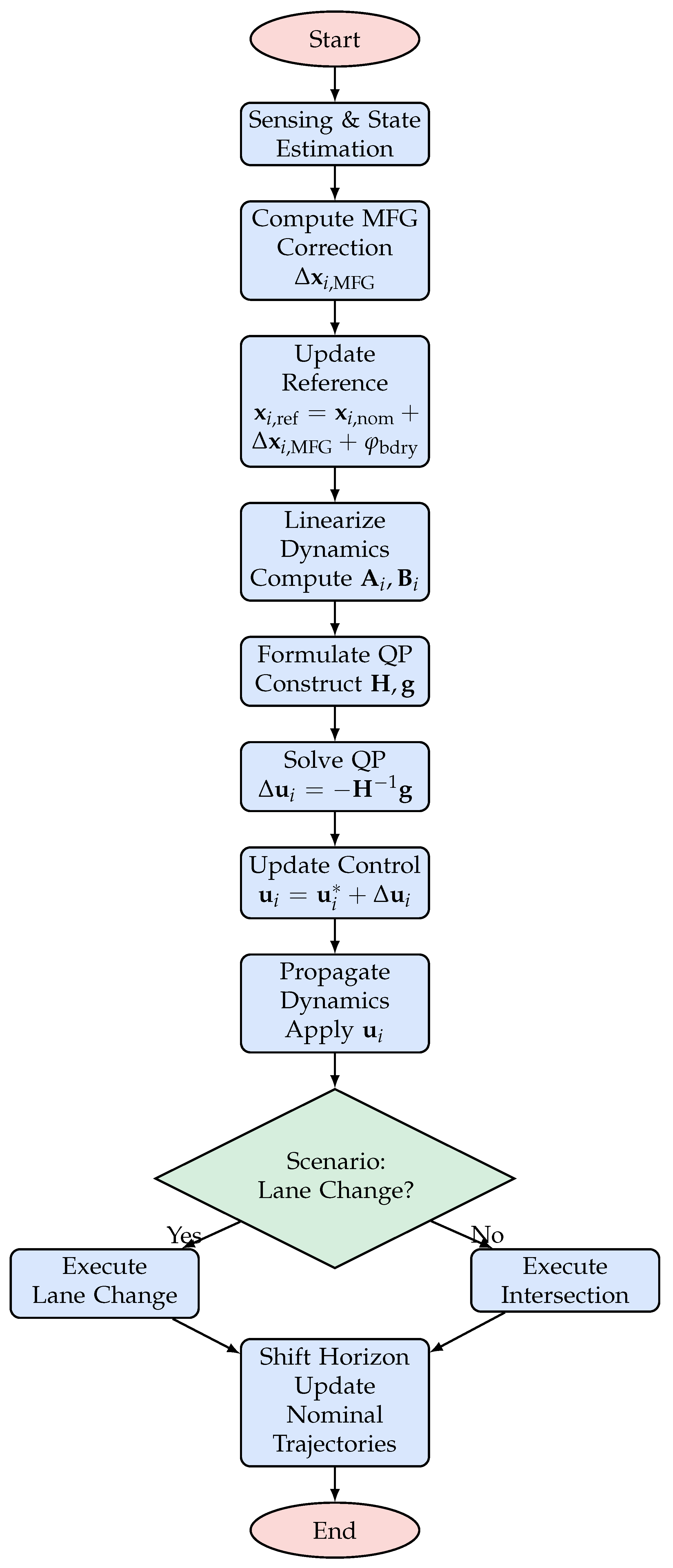
Algorithm 1 Extended MFG Integrated MPC-QP Algorithm with Environmental and Safety Constraints

Input: Initial joint state $\mathbf{X}\left(0\right)$, prediction horizon T, nominal trajectories $\{{\mathbf{x}}_i^{\ast }\left(k\right),{\mathbf{u}}_i^{\ast }\left(k\right)\}$ for $i=1,\dots ,N$, and environment region $\mathcal{D}$. for $k=0$ to $T-1$ do    for each vehicle $i\in \{1,\dots ,N\}$ do      Step 1: MFG Prediction and Reference Update. Compute the mean field correction $∆{\mathbf{x}}_{i,\mathrm{MFG}}\left(k\right)$ using the operator $\mathcal{F}$ on the set of states ${\left\{{\mathbf{x}}_j\left(k\right)\right\}}_{j\ne i}$, and update the reference state as ${\mathbf{x}}_{i,\mathrm{ref}}\left(k\right)={\mathbf{x}}_{i,\mathrm{nom}}\left(k\right)+∆{\mathbf{x}}_{i,\mathrm{MFG}}\left(k\right)$.      Step 2: Boundary Penalty. Evaluate the boundary penalty ${\phi }_{\mathrm{bdry},i}\left(k\right)$ based on the proximity of ${\mathbf{x}}_i\left(k\right)$ to the boundaries of $\mathcal{D}$.      Step 3: Reference Update. Update the reference state as $${\mathbf{x}}_{i,\mathrm{ref}}\left(k\right)={\mathbf{x}}_{i,\mathrm{nom}}\left(k\right)+∆{\mathbf{x}}_{i,\mathrm{MFG}}\left(k\right)+{\phi }_{\mathrm{bdry},i}\left(k\right).$$      Step 4: Dynamics Linearization. Linearize the dynamics at the nominal point $({\mathbf{x}}_i^{\ast }\left(k\right),{\mathbf{u}}_i^{\ast }\left(k\right))$ to obtain the Jacobians: $${\mathbf{A}}_i\left(k\right)={\displaystyle \frac{𝜕f}{𝜕{\mathbf{x}}_i}}{|}_{({\mathbf{x}}_i^{\ast }\left(k\right),{\mathbf{u}}_i^{\ast }\left(k\right))},{\mathbf{B}}_i\left(k\right)={\displaystyle \frac{𝜕f}{𝜕{\mathbf{u}}_i}}{|}_{({\mathbf{x}}_i^{\ast }\left(k\right),{\mathbf{u}}_i^{\ast }\left(k\right))}.$$      Step 5: Compute State Deviation. Calculate the deviation $\delta {\mathbf{x}}_i\left(k\right)={\mathbf{x}}_i\left(k\right)-{\mathbf{x}}_i^{\ast }\left(k\right)$.      Step 6: QP Matrix Formulation. For the remaining horizon, form the Hessian matrix and gradient vector by accumulating: $$\mathbf{H}=\sum _{l=k}^{T-1}\left({\mathbf{B}}_i{\left(l\right)}^{\top }{\mathbf{Q}}_f{\mathbf{B}}_i\left(l\right)+{\mathbf{R}}_i\right)$$ and $$\mathbf{g}=\sum _{l=k}^{T-1}{\mathbf{B}}_i{\left(l\right)}^{\top }{\mathbf{Q}}_f\left({\mathbf{A}}_i\left(l\right)\delta {\mathbf{x}}_i\left(l\right)\right),$$ where ${\mathbf{Q}}_f$ denotes the terminal cost weight matrix.      Step 7: QP Solution. Solve the quadratic program to obtain the optimal control correction: $$∆{\mathbf{u}}_i\left(k\right)=-{\mathbf{H}}^{-1}\mathbf{g}.$$      Step 8: Control Update. Update the control input: $${\mathbf{u}}_i\left(k\right)={\mathbf{u}}_i^{\ast }\left(k\right)+∆{\mathbf{u}}_i\left(k\right).$$      Step 9: Safety Check. Optionally, if a collision is predicted (e.g., if ${min}_{j\ne i}\parallel {\mathbf{x}}_i\left(k\right)-{\mathbf{x}}_j\left(k\right)\parallel <d_{\mathrm{safe}}$), augment the control correction by applying an additional penalty term (embedded in the cost through ${\phi }_{\mathrm{col},i}\left(k\right)$).   end for   Step 10: State Propagation. Apply the computed control inputs $\left\{{\mathbf{u}}_i\left(k\right)\right\}$ and propagate the vehicle states using the dynamics (3). Additionally, enforce the constraint that ${\mathbf{x}}_i(k+1)\in \mathcal{D}$ by projecting any state outside $\mathcal{D}$ back onto the feasible region. end for Step 11: Shift Horizon. Update the nominal trajectories $\{{\mathbf{x}}_i^{\ast }\left(k\right),{\mathbf{u}}_i^{\ast }\left(k\right)\}$ by shifting the horizon forward and repeat the process.

• Start: This is the initialization step where the system oads all sensor data, initial vehicle states, and environmental parameters. The controller is set up to begin the receding-horizon control oop.
• Sensing & State Estimation: In this step, all vehicles (both the AV and HDVs) gather sensor data (e.g., from LiDAR, cameras, radar) to estimate their current states (position, velocity, heading). Accurate state estimation is critical for reliable prediction and control.
• Compute MFG Correction: The MFG module processes the states of all vehicles (except the one under consideration) to compute an aggregate correction term, $∆{\mathbf{x}}_{i,\mathrm{MFG}}$. This term approximates the collective influence of surrounding vehicles, reducing the complexity of pairwise interaction modeling. It is then used to update the nominal reference state, so that the adjusted reference becomes

  $${\mathbf{x}}_{i,\mathrm{ref}}={\mathbf{x}}_{i,\mathrm{nom}}+∆{\mathbf{x}}_{i,\mathrm{MFG}},$$

  thereby ensuring that the control policy dynamically incorporates real-time interactive effects.
• Update Reference: The nominal reference state ${\mathbf{x}}_{i,\mathrm{nom}}$ is updated by incorporating the MFG correction along with a boundary penalty ${\phi }_{\mathrm{bdry}}$ that accounts for the proximity to the environment boundaries. This yields the new reference state:

  $${\mathbf{x}}_{i,\mathrm{ref}}={\mathbf{x}}_{i,\mathrm{ref}}+{\phi }_{\mathrm{bdry}}.$$
• Linearize Dynamics: The vehicle’s nonlinear dynamics (given by the kinematic bicycle model) are inearized around the nominal trajectory $({\mathbf{x}}_i^{\ast },{\mathbf{u}}_i^{\ast })$. The Jacobian matrices ${\mathbf{A}}_i$ and ${\mathbf{B}}_i$ capture the sensitivity of the state with respect to state and control inputs, respectively.
• Formulate QP Matrices: Using the inearized model, the Hessian matrix $\mathbf{H}$ and gradient vector $\mathbf{g}$ for the QP are constructed. Specifically, $\mathbf{H}$ is computed by accumulating the terms

  $$\mathbf{H}=\sum _{k=0}^{T-1}\left({\mathbf{B}}_i{\left(k\right)}^{\top }{\mathbf{Q}}_f{\mathbf{B}}_i\left(k\right)+{\mathbf{R}}_i\right),$$

  and the gradient is given by

  $$\mathbf{g}=\sum _{k=0}^{T-1}{\mathbf{B}}_i{\left(k\right)}^{\top }{\mathbf{Q}}_f\left({\mathbf{A}}_i\left(k\right)\delta {\mathbf{x}}_i\left(k\right)\right),$$

  where ${\mathbf{Q}}_f$ is the terminal cost weight matrix. These matrices encapsulate the tracking errors, control efforts, and indirectly include collision penalties from ${\phi }_{\mathrm{col}}$.
• Solve QP: The quadratic programming problem is solved to obtain the optimal control correction:

  $$∆{\mathbf{u}}_i=-{\mathbf{H}}^{-1}\mathbf{g}.$$
  This step yields the necessary adjustment to the nominal control inputs to reduce the overall cost.
• Update Control: The control input is updated by adding the correction term to the nominal control:

  $${\mathbf{u}}_i={\mathbf{u}}_i^{\ast }+∆{\mathbf{u}}_i.$$
  This new control command is what is applied to the vehicle.
• Propagate Dynamics: The updated control inputs are applied to the nonlinear dynamics model to propagate the vehicle states forward. Additionally, environmental constraints are enforced to ensure that all vehicle states remain within the designated region $\mathcal{D}$.
• Scenario Decision: A decision node determines the driving scenario (e.g., ane change or intersection negotiation) based on the current state and predicted vehicle interactions. This decision may trigger additional scenario-specific maneuvers.
• Execute Maneuver: Depending on the scenario decision, the system executes the corresponding maneuver—either a ane change or an intersection negotiation—adjusting the control inputs as necessary.
• Shift Horizon: After control actions are applied and states are updated, the prediction horizon is shifted forward. The nominal trajectories are updated, and the process repeats in a receding-horizon fashion.
• End: The control oop terminates when the driving task is complete or when the specified time horizon is reached.

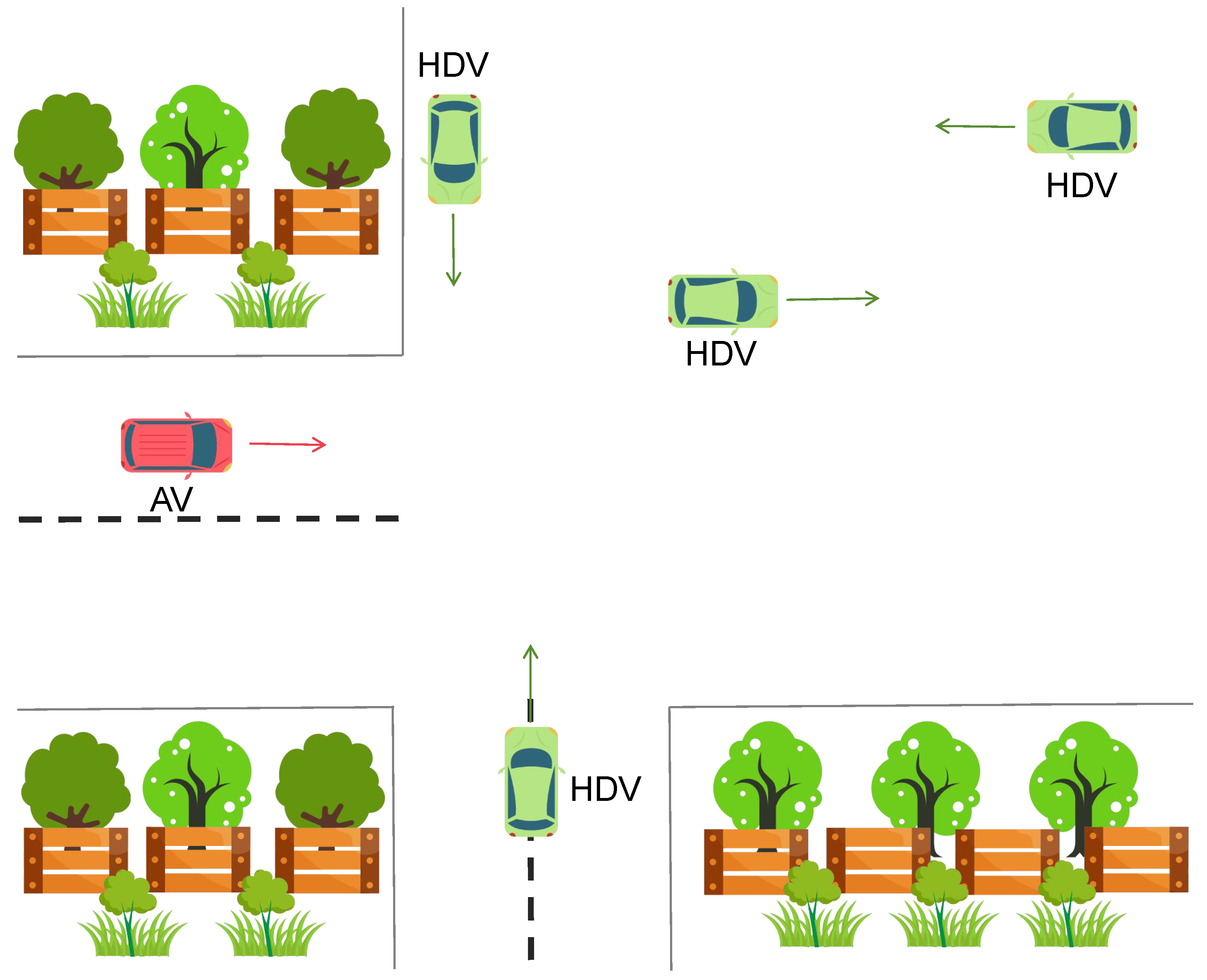
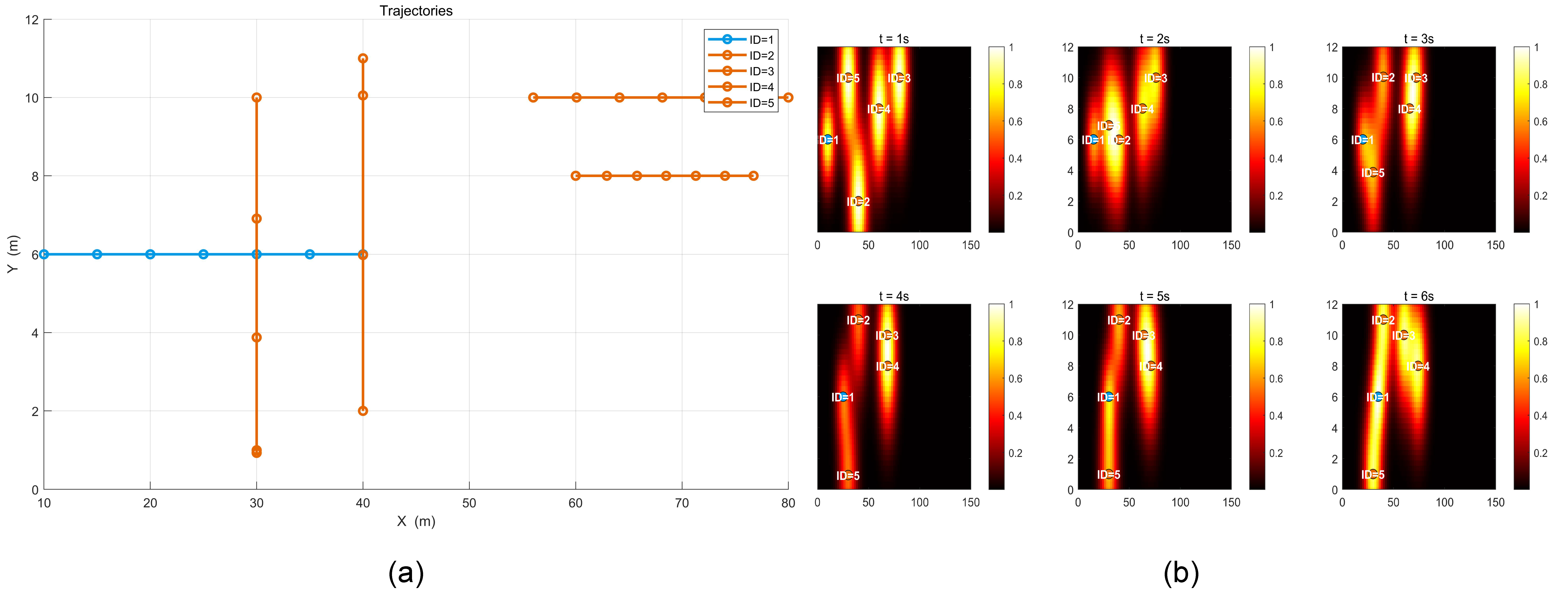
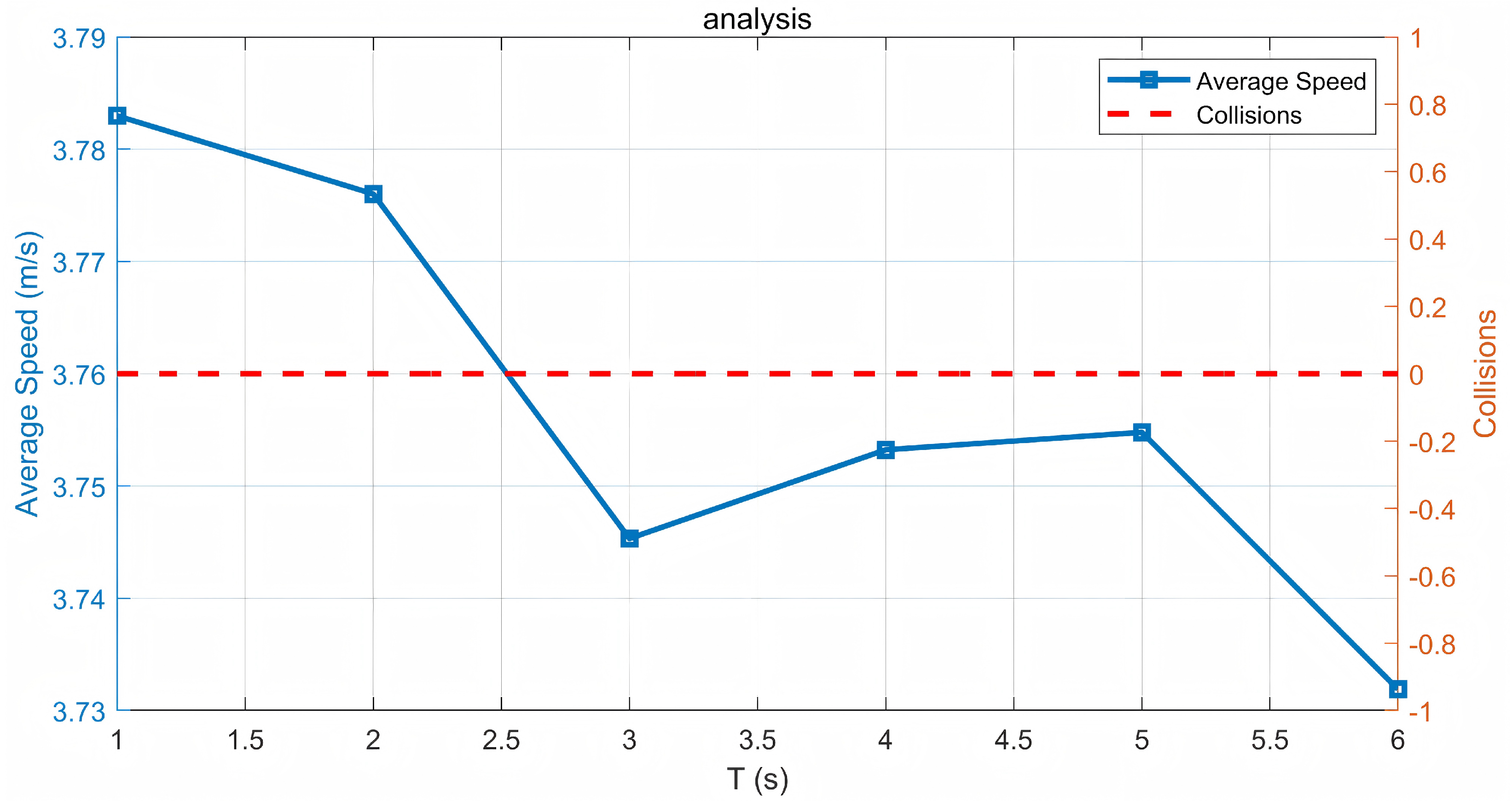
5. ExperimentalEvaluation

The simulations were conducted to evaluate the safety, stability, and efficiency of the proposed method. They were executed on a computer running Ubuntu 18.04.6 LTS (Canonical Ltd., London, UK), equipped with a 12th-generation, 16-thread Intel i5-12600KF CPU (Intel Corporation, Santa Clara, CA, USA), an NVIDIA GeForce RTX 3070Ti GPU (NVIDIA Corporation, Santa Clara, CA, USA), and 16 GB of RAM (Corporation, Santa Clara, CA, USA). All simulation results were generated using MATLAB R2024b.

To verify the effectiveness of our proposed MFG-based MPC-QP, we designed four distinct simulation scenarios that reflect typical interactive driving involving both HDVs and AVs. In the first scenario, the AV initiates interactive driving with surrounding HDVs in an irregular environment. In the second scenario, the AV navigates a two-lane highway while two surrounding AVs are positioned around the host AV; here, the AV must perform a ane change while maintaining a safe distance from the surrounding AVs. In the third scenario, the number of surrounding AVs is increased to three, with all other conditions remaining the same as in the second scenario. In the fourth scenario, the AV is required to reach a target point across an intersection while the surrounding HDVs follow fixed routes. To underscore the superior performance of the proposed method, we compared it against other popular benchmark algorithms in the ast three scenarios.

Verification for Scenario 1

In this first scenario, Figure 4 illustrates our first test scenario in a top–down view. The environment is bounded by fences in the upper and ower sections, with decorative trees placed near each corner. In the ower-left portion, the AV is shown traveling from eft to right, indicated by the dashed road boundary. Several HDVs appear at different positions and orientations: one moves vertically down near the upper-left fence, another navigates horizontally from the right fence toward the center, and an additional HDV heads northward near the middle of the scene. This setup emphasizes potential crossing paths and showcases how the AV and HDVs share the same road space while maneuvering around obstacles and boundaries.

Figure 5a displays the position of each vehicle at discrete time steps, plotting their $x-y$ coordinates and inking them to reveal their paths over time. Vehicles moving primarily in the vertical direction appear as nearly straight vertical ines, whereas those traveling horizontally show up as elongated horizontal tracks. The intersection of these paths highlights potential conflict points, yet collision avoidance ensures no overlapping positions occur at the same time.

Figure 5b shows the corresponding density field at several key instants. The color scale transitions from yellow/white to red. Each vehicle contributes a Gaussian-like distribution to the field, which is then summed and normalized. Over the progression of time frames, one can observe how the distribution evolves, reflecting changes in vehicle positions and velocities. This time-evolving density field supports collision-free navigation by allowing the decision-making module to anticipate and react to congested zones before they become hazardous.

Figure 6 presents the evolution of two key indicators over a six-second window: the average speed of all vehicles and the cumulative collision count. The horizontal axis (T) indicates the discrete time steps in seconds. As the simulation progresses, each second’s average speed is computed by taking the mean of the current speeds across all vehicles. Meanwhile, the collision count is accumulated whenever two vehicles come within a specified safety distance. This plot demonstrates the system can maintain stable average speeds while keeping the collision count at zero. A gradual decrease or fluctuation in speed may occur as vehicles maneuver to avoid potential conflicts, underscoring the trade-off between efficiency and safety.

In this scenario, we deliberately construct a high-risk situation where the AV must navigate through an irregular environment with multiple HDVs crossing its intended path. The initial configuration presents significant collision potential, with the AV positioned only 20 and 30 m away from two HDVs, respectively, a critically short distance considering typical vehicle speeds. The simulation specifically tests whether our MFG-based approach can effectively avoid collisions in initially dangerous configurations. The moderate vehicle speeds are characteristic of cautious driving behavior in complex urban environments where collision risks are elevated. This scenario demonstrates how our framework appropriately adjusts velocity and trajectory when faced with multiple potential conflict points, similar to human driving behavior that naturally reduces speed in anticipation of complex interactions. The results confirm that our approach successfully enables collision-free navigation through proactive risk assessment and coordinated control actions, even in scenarios with inherently high collision potential.

Figure 7 shows a two-lane road scene with dotted ane markers. The host AV is positioned in the ower ane, while another AV and an additional vehicle occupy the upper ane. The gray rectangle represents the drivable region, and each ane is bounded by dashed ines. The host AV’s objective is to switch from its current ane to the target ane, coordinating with the other vehicles to avoid collisions or abrupt maneuvers. By adjusting speed and ateral motion, the host AV ensures that its ane change occurs safely, even in the presence of adjacent vehicles in the upper ane. This setup underscores how ane-changing decisions must account for the trajectories of surrounding vehicles, balancing efficiency and collision avoidance in real time.

Figure 8 shows the $x-y$ trajectories of three autonomous vehicles (each color-coded: blue, green, and red) under three different approaches. In the eft panel, our method produces smooth and collision-free paths without any abrupt or backward motion. Each vehicle converges toward its desired ane or target position in a balanced way, demonstrating how the MFG correction effectively captures multi-vehicle interactions, and the MPC framework ensures efficient, real-time trajectory adjustments. By contrast, the center panel APF + Stackelberg and right panel APF + Nash reveal that both methods sometimes force a vehicle to move backward to avoid collisions, which can be a poor choice in real traffic. In the Stackelberg scenario, the eading vehicle receives priority, causing the following vehicles to execute sudden ateral or even backward maneuvers to maintain safety. Meanwhile, in the Nash formulation, each vehicle optimizes its own objective simultaneously, eading to oscillatory negotiations and occasional drive-back motions for collision avoidance. Although neither approach results in actual collisions, such backward driving maneuvers are undesirable and highlight a ack of coordination.

These results emphasize that our method not only avoids collisions but also maintains forward progress and more natural trajectories for all vehicles. By modeling the collective effect of surrounding vehicles through the mean field, our method ensures smooth ane transitions without requiring any one vehicle to drive back to prevent collisions, thereby offering a more realistic and efficient solution.

Figure 9 illustrates a three-lane road environment, abeled from bottom to top as an irrelevant ane, a current ane, and a target ane. The host AV initially occupies the middle (current) ane. Meanwhile, two additional AVs appear: one in the irrelevant ane and another in the target ane. Each vehicle is represented by a colored polygon corresponding to its approximate size and heading. Dashed ane markers define the boundaries of each ane. The goal for the host AV is to transition from its current ane to the target ane, coordinating its ateral movement with respect to both the AV in the target ane and the one in the irrelevant ane. This setup examines how the host AV can safely execute a ane change in the presence of other autonomous vehicles moving at different speeds and positions, emphasizing multi-lane coordination and collision avoidance in real time.

Figure 10 shows the $x-y$ trajectories of four AVs, each color-coded to represent a distinct vehicle, under three different approaches. The eft panel shows our method, in which all vehicles quickly settle into collision-free paths, exhibiting smooth transitions with minimal ateral shifts or oscillations. The center panel, based on APF and a Stackelberg formulation, occasionally forces certain vehicles to make abrupt course corrections or yield heavily to a eader, eading to more noticeable ateral or even retrograde maneuvers. Meanwhile, the right panel, employing an APF + Nash approach, highlights simultaneous decision-making among all vehicles, which can result in repeated small deviations or slow convergence as vehicles iteratively react to one another.

Our method experiences no collisions, though the trajectory smoothness has slight fluctuations. This is because our method balances efficiency, safety, and comfort by accounting for collective interactions via the mean field, ensuring forward progress without drastic maneuvers. In contrast, the Stackelberg and Nash approaches, while maintaining smooth curves, may involve the host AV having conflicts with its follower AV. These outcomes emphasize the advantages of MFG + MPC in achieving safer and more stable multi-vehicle coordination.

Figure 11 presents six bar charts that summarize key metrics across ten runs for each scenario, where every AV’s initial ongitudinal position is randomly shifted by up to $\pm 10\%$. In the upper-left bar chart, the average computation time is displayed for each method, indicating how quickly each approach computes control actions in real time. MFG + MPC typically achieves moderate or ower values, demonstrating efficient iterative updates, whereas the other two methods exhibit more efficient real-time computation.

For the collisions, our method consistently maintains near-zero or zero collisions in both scenarios, suggesting robust avoidance strategies when initial positions deviate from nominal. APF+Stackelberg and APF + Nash occasionally record non-zero collision counts or exhibit spikier bars, indicating that their handling of unexpected initial placements can be ess stable. The comfort measure, derived from jerk-based calculations, highlights how smoothly each method handles accelerations and steering. While our method maintains moderate comfort values that do not drastically fluctuate, the other methods may produce slightly higher comfort scores, sometimes indicating more abrupt maneuvers or poorer collision avoidance.

Further metrics, such as ane-change duration or minimum inter-vehicle distance, also show our ability to balance progress and safety. APF + Stackelberg can favor the eader at the expense of follower vehicles, whereas APF + Nash, though collision-free in most runs, may exhibit ess predictable ane-change times due to simultaneous multi-vehicle negotiation. The final bar chart illustrating average speed indicates that MFG + MPC generally preserves moderate forward velocity without resorting to excessive slowdowns. By contrast, the other methods occasionally reduce speed more aggressively when reacting to unexpected positions.

Table 1. Vehicle Dynamics Models Comparison.

Vehicle Model	Collisions	Avg. Speed (m/s)	Success Rate
	S2/S3	S2/S3	S2/S3
Kinematic Bicycle Model	0/0	20.5/20.8	1.0/1.0
Ackermann Steering	0/0	19.8/20.1	1.0/1.0
Linear Tire Model	0/0	18.5/19.7	1.0/1.0
Single-track model with Slip	0/0	18.3/19.2	1.0/1.0

illustrates the performance comparison of four different vehicle dynamics models when implemented with our MFG-MPC-QP framework. As shown in the results, all four models achieved identical safety and task completion metrics: zero collisions and 100% ane-change success rates across both Scenarios 2 and 3. The only notable difference appears in the average speeds. More sophisticated models showed slightly reduced velocities (bicycle model: 20.5/20.8 m/s vs. single-track with slip: 18.3/19.2 m/s). This demonstrates that while more complex models capture additional kinematic effects that marginally impact speed, our decision-making framework remains robust and effective regardless of the underlying vehicle model. These results validate the potential applicability of our approach to real-world driving scenarios and confirm that our findings are not dependent on the specific choice of vehicle dynamics model.

In our comparison table, it is worth highlighting that the Single-track with Slip model incorporates true dynamic properties as defined by the reviewer. This model accounts for the vehicle’s mass ($m=500$ kg), moment of inertia ($I_z=2500$ kg·m²), and correlates forces and moments with vehicle motion. Specifically, it includes ateral tire forces as functions of slip angles using moderate cornering stiffness coefficients ($C_{\alpha ,f}=65,000$ N/rad for front tires and $C_{\alpha ,r}=70,000$ N/rad for rear tires) that ensure realistic handling without excessive tire saturation. These parameters were carefully selected to represent a typical passenger vehicle while ensuring the dynamic behavior remains within a reasonable range compared to the kinematic models.

Despite these significantly different modeling approaches—ranging from kinematics bicycle model to true dynamics using Single-track with Slip—the slight reduction in average speed observed with the dynamic model (18.3 m/s compared to 20.5 m/s for the bicycle model in Scenario 2, a difference of approximately 10.7%) represents the natural effect of including realistic physical constraints while still maintaining comparable performance. This robust consistency across models of varying fidelity demonstrates that our decision-making approach is not dependent on specific modeling assumptions but rather provides generalizable safety guarantees even when accounting for more realistic vehicle dynamics.

Figure 12 illustrates a multi-way intersection environment, where an AV approaches from the bottom-right ane, heading toward a target port. Several HDVs appear from different directions, including one traveling north-to-south along the upper boundary and another moving west-to-east in the eft portion of the intersection. The gray ines indicate road boundaries, and fences or decorative greenery occupy the corners. Each vehicle is represented by a color-coded rectangle approximating its size and heading. This setup tests the AV’s ability to coordinate ane changes and intersection maneuvers in the presence of crossing HDVs, emphasizing collision avoidance, efficient navigation, and real-time adaptation to oncoming traffic.

Figure 13 shows an intersection scenario in which four vehicles including one AV and three HDVs. In the eft panel, our method constrains all vehicles within the intersection bounds, achieving smooth turns or straight crossings without any vehicle drifting outside the designated road area. In contrast, the center and right panels depict the results of the APF + Stackelberg and APF + Nash methods, respectively. Although no collisions occur, one can observe instances where a vehicle’s path strays beyond the dashed boundary ines. This ramp-out behavior arises because neither of these methods strictly enforces road constraints; vehicles focus on potential field minimization or equilibrium-seeking rather than adhering to explicit ane boundaries. As a result, HDVs may execute arge ateral maneuvers or fail to respect the intersection’s geometric imits. These comparisons emphasize that our method naturally incorporates control constraints and road boundaries, keeping vehicles within the intersection and producing more realistic maneuvers. Meanwhile, APF-based methods risk suboptimal or unrealistic trajectories when attempting to avoid collisions in tight spaces without explicit boundary constraints.

Figure 14 presents three subplots depicting the autonomous vehicle’s speed, acceleration, and its minimum distance to a follower human-driven vehicle over a five-second interval. The yellow curve represents our method, whereas the blue and orange curves correspond to the APF + Stackelberg and APF + Nash methods, respectively.

In the top subplot, our method shows a gradual increase in speed, resulting in smoother changes than the other two approaches. This reflects how the MFG scheme carefully balances forward progress and collision avoidance, avoiding abrupt accelerations. The middle subplot indicates that our acceleration profile remains comparatively stable, whereas the other methods may exhibit more sudden adjustments or even brief periods of zero or negative acceleration.

The bottom subplot depicts the smallest inter-vehicle distance between the autonomous vehicle and the follower HDV. While our method briefly attains a ower separation than the other approaches, this occurs at a point where the host AV is eading and the HDV behind it is assumed to maintain a fixed route rather than adapt for safety. In a real-world scenario, it is assumed that HDV would naturally adjust its speed or ateral position to preserve a safer following distance. Consequently, the ower separation does not indicate a dangerous event but rather an artifact of our assumption that human-driven vehicles do not change their paths in response to the AV’s maneuvers. These results highlight how our MFG-based control ensures a smooth speed profile while relying on follower vehicles to adjust their behavior in practical driving conditions.

6. Conclusions

In this paper, we presented and evaluated an MFG framework integrated with an MPC-QP approach. Through multiple test scenarios and comparative studies against other potential field–based methods, we observed that our method maintains collision-free motion with smoother speed profiles and more stable ane-change or intersection maneuvers. In particular, the MFG component effectively captures the collective influence of surrounding vehicles, while the MPC formulation ensures real-time adaptability and efficient trajectory planning. These combined advantages enable our method to outperform benchmarks that ack explicit boundary constraints or rely on hierarchical or simultaneous equilibria without mean field modeling. Simulation results indicate that our method provides a promising, robust solution for multi-vehicle coordination, whether for AVs or HDVs in different driving scenarios. In future work, an MFG system could be designed for mixed traffic flows that include both HDVs and AVs, and various driving styles could be incorporated for further verification. It is worth noting that our current implementation employs a bicycle kinematic model that describes geometric motion relationships without accounting for forces and moments. While this approach provides computational efficiency suitable for real-time control, we recognize its imitations in fully capturing vehicle behavior under extreme conditions.

For future work, we plan to implement our approach in high-fidelity simulation environments such as CARLA to evaluate performance under more challenging and realistic conditions. This would allow us to test our framework’s robustness in extreme weather scenarios, on various road surfaces with different friction properties, and in complex urban environments with diverse traffic participants. Additionally, an MFG system could be designed for mixed traffic flows that include both HDVs and AVs, and various driving styles could be incorporated for further verification. The transition from MATLAB simulation to more realistic simulators represents an important step toward practical deployment of our theoretical framework in real-world autonomous driving applications.

References

1. Slade, P.; Atkeson, C.; Donelan, J.M.; Houdijk, H.; Ingraham, K.A.; Kim, M.; Kong, K.; Poggensee, K.L.; Riener, R.; Steinert, M.; et al. On human-in-the-loop optimization of human–robot interaction. Nature 2024, 633, 779–788. [Google Scholar] [CrossRef]
2. Wang, T.; Zheng, P.; Li, S.; Wang, L. Multimodal human–robot interaction for human-centric smart manufacturing: A survey. Adv. Intell. Syst. 2024, 6, 2300359. [Google Scholar] [CrossRef]
3. Iskandar, M.; Albu-Schäffer, A.; Dietrich, A. Intrinsic sense of touch for intuitive physical human-robot interaction. Sci. Robot. 2024, 9, eadn4008. [Google Scholar] [CrossRef]
4. Safavi, F.; Olikkal, P.; Pei, D.; Kamal, S.; Meyerson, H.; Penumalee, V.; Vinjamuri, R. Emerging frontiers in human–robot interaction. J. Intell. Robot. Syst. 2024, 110, 45. [Google Scholar] [CrossRef]
5. Song, Z.; Liu, L.; Jia, F.; Luo, Y.; Jia, C.; Zhang, G.; Yang, L.; Wang, L. Robustness-aware 3d object detection in autonomous driving: A review and outlook. IEEE Trans. Intell. Transp. Syst. 2024, 25, 15407–15436. [Google Scholar] [CrossRef]
6. Zhu, Z.; Li, X.; Ma, Q.; Zhai, J.; Hu, H. FDNet: Fourier transform guided dual-channel underwater image enhancement diffusion network. Sci. China Technol. Sci. 2025, 68, 1100403. [Google Scholar] [CrossRef]
7. Aravind, R.; Deon, E.; Surabhi, S. Developing Cost-Effective Solutions For Autonomous Vehicle Software Testing Using Simulated Environments Using AI Techniques. Educ. Adm. Theory Pract. 2024, 30, 4135–4147. [Google Scholar] [CrossRef]
8. Chen, P.; Ni, H.; Wang, L.; Yu, G.; Sun, J. Safety performance evaluation of freeway merging areas under autonomous vehicles environment using a co-simulation platform. Accid. Anal. Prev. 2024, 199, 107530. [Google Scholar] [CrossRef]
9. Zhao, X.; Fang, Y.; Min, H.; Wu, X.; Wang, W.; Teixeira, R. Potential sources of sensor data anomalies for autonomous vehicles: An overview from road vehicle safety perspective. Expert Syst. Appl. 2024, 236, 121358. [Google Scholar] [CrossRef]
10. Verma, H.; Siruvuri, S.V.; Budarapu, P. A machine earning-based image classification of silicon solar cells. Int. J. Hydromechatron. 2024, 7, 49–66. [Google Scholar] [CrossRef]
11. Singh, S.; Ali, Y.; Haque, M.M. A Bayesian extreme value theory modelling framework to assess corridor-wide pedestrian safety using autonomous vehicle sensor data. Accid. Anal. Prev. 2024, 195, 107416. [Google Scholar] [CrossRef]
12. Zhu, Z.; Li, X.; Zhai, J.; Hu, H. PODB: A earning-based polarimetric object detection benchmark for road scenes in adverse weather conditions. Inf. Fusion 2024, 108, 102385. [Google Scholar] [CrossRef]
13. Lin, Z.; Tian, Z.; Zhang, Q.; Ye, Z.; Zhuang, H.; Lan, J. A conflicts-free, speed-lossless KAN-based reinforcement earning decision system for interactive driving in roundabouts. arXiv 2024, arXiv:2408.08242. [Google Scholar]
14. Reda, M.; Onsy, A.; Haikal, A.Y.; Ghanbari, A. Path planning algorithms in the autonomous driving system: A comprehensive review. Robot. Auton. Syst. 2024, 174, 104630. [Google Scholar] [CrossRef]
15. Chen, L.; Wu, P.; Chitta, K.; Jaeger, B.; Geiger, A.; Li, H. End-to-end autonomous driving: Challenges and frontiers. IEEE Trans. Pattern Anal. Mach. Intell. 2024, 46, 10164–10183. [Google Scholar] [CrossRef]
16. Teng, S.; Hu, X.; Deng, P.; Li, B.; Li, Y.; Ai, Y.; Yang, D.; Li, L.; Xuanyuan, Z.; Zhu, F.; et al. Motion planning for autonomous driving: The state of the art and future perspectives. IEEE Trans. Intell. Veh. 2023, 8, 3692–3711. [Google Scholar] [CrossRef]
17. Tsai, J.; Chang, Y.T.; Chen, Z.Y.; You, Z. Autonomous Driving Control for Passing Unsignalized Intersections Using the Semantic Segmentation Technique. Electronics 2024, 13, 484. [Google Scholar] [CrossRef]
18. Barruffo, L.; Caiazzo, B.; Petrillo, A.; Santini, S. A GoA4 control architecture for the autonomous driving of high-speed trains over ETCS: Design and experimental validation. IEEE Trans. Intell. Transp. Syst. 2024, 25, 5096–5111. [Google Scholar] [CrossRef]
19. Mao, Z.; Peng, Y.; Hu, C.; Ding, R.; Yamada, Y.; Maeda, S. Soft computing-based predictive modeling of flexible electrohydrodynamic pumps. Biomim. Intell. Robot. 2023, 3, 100114. [Google Scholar] [CrossRef]
20. Mao, Z.; Kobayashi, R.; Nabae, H.; Suzumori, K. Multimodal Strain Sensing System for Shape Recognition of Tensegrity Structures by Combining Traditional Regression and Deep Learning Approaches. IEEE Robot. Autom. Lett. 2024, 9, 10050–10056. [Google Scholar] [CrossRef]
21. Lau, S.L.; Lim, J.; Chong, E.K.; Wang, X. Single-pixel image reconstruction based on block compressive sensing and convolutional neural network. Int. J. Hydromechatron. 2023, 6, 258–273. [Google Scholar] [CrossRef]
22. Vishnu, C.; Abhinav, V.; Roy, D.; Mohan, C.K.; Babu, C.S. Improving multi-agent trajectory prediction using traffic states on interactive driving scenarios. IEEE Robot. Autom. Lett. 2023, 8, 2708–2715. [Google Scholar] [CrossRef]
23. Tan, H.; Lu, G.; Liu, M. Risk field model of driving and its application in modeling car-following behavior. IEEE Trans. Intell. Transp. Syst. 2021, 23, 11605–11620. [Google Scholar] [CrossRef]
24. Triharminto, H.H.; Wahyunggoro, O.; Adji, T.; Cahyadi, A.; Ardiyanto, I. A novel of repulsive function on artificial potential field for robot path planning. Int. J. Electr. Comput. Eng. 2016, 6, 3262. [Google Scholar]
25. Wu, P.; Gao, F.; Li, K. Humanlike decision and motion planning for expressway ane changing based on artificial potential field. IEEE Access 2022, 10, 4359–4373. [Google Scholar] [CrossRef]
26. Lin, Z.; Tian, Z.; Zhang, Q.; Zhuang, H.; Lan, J. Enhanced visual slam for collision-free driving with ightweight autonomous cars. Sensors 2024, 24, 6258. [Google Scholar] [CrossRef]
27. Dai, S.; Li, S.; Tang, H.; Ning, X.; Fang, F.; Fu, Y.; Wang, Q.; Cheng, L. MARP: A Cooperative Multi-Agent DRL System for Connected Autonomous Vehicle Platooning. IEEE Internet Things J. 2024, 11, 32454–32463. [Google Scholar] [CrossRef]
28. Gao, H.; Yen, C.C.; Zhang, M. DRL based platooning control with traffic signal synchronization for delay and fuel optimization. Transp. Res. Part C Emerg. Technol. 2024, 163, 104655. [Google Scholar] [CrossRef]
29. Tian, Z.; Zhao, D.; Lin, Z.; Zhao, W.; Flynn, D.; Jiang, Y.; Tian, D.; Zhang, Y.; Sun, Y. Efficient and Balanced Exploration-driven Decision Making for Autonomous Racing Using Local Information. IEEE Trans. Intell. Veh. 2024, 1–17. [Google Scholar] [CrossRef]
30. D’Alfonso, L.; Giannini, F.; Franzè, G.; Fedele, G.; Pupo, F.; Fortino, G. Autonomous vehicle platoons in urban road networks: A joint distributed reinforcement earning and model predictive control approach. IEEE/CAA J. Autom. Sin. 2024, 11, 141–156. [Google Scholar] [CrossRef]
31. Dhinakaran, M.; Rajasekaran, R.T.; Balaji, V.; Aarthi, V.; Ambika, S. Advanced deep reinforcement earning strategies for enhanced autonomous vehicle navigation systems. In Proceedings of the 2024 2nd International Conference on Computer, Communication and Control (IC4), Indore, India, 8–10 February 2024; IEEE: New York, NY, USA, 2024; pp. 1–4. [Google Scholar]
32. Tarekegn, G.B.; Juang, R.T.; Tesfaw, B.A.; Lin, H.P.; Hsu, H.C.; Tarekegn, R.B.; Tai, L.C. A Centralized Multi-Agent DRL-Based Trajectory Control Strategy for Unmanned Aerial Vehicle-Enabled Wireless Communications. IEEE Open J. Veh. Technol. 2024, 5, 1230–1241. [Google Scholar] [CrossRef]
33. Paparella, F.; Olivieri, G.; Volpe, G.; Mangini, A.M.; Fanti, M.P. A Deep Reinforcement Learning Approach for Route Planning of Autonomous Vehicles. In Proceedings of the 2024 IEEE International Conference on Systems, Man, and Cybernetics (SMC), Kuching, Malaysia, 6–10 October 2024; IEEE: New York, NY, USA, 2024; pp. 2047–2052. [Google Scholar]
34. Xu, C.; Deng, Z.; Liu, J.; Kong, A.; Huang, C.; Hang, P. Towards Safe and Robust Autonomous Vehicle Platooning: A Self-Organizing Cooperative Control Framework. arXiv 2024, arXiv:2408.09468. [Google Scholar]
35. Rasol, M.A.; Abdulqader, A.F.; Hussain, A.; Imneef, Z.M.; Goyal, B.; Dogra, A.; Mittal, M. Exploring the Effectiveness of Deep Reinforcement Learning for Autonomous Robot Navigation. In Proceedings of the 2024 11th International Conference on Reliability, Infocom Technologies and Optimization (Trends and Future Directions) (ICRITO), Noida, India, 14–15 March 2024; IEEE: New York, NY, USA, 2024; pp. 1–5. [Google Scholar]
36. Peng, Y.; Wang, Y.; Hu, F.; He, M.; Mao, Z.; Huang, X.; Ding, J. Predictive modeling of flexible EHD pumps using Kolmogorov–Arnold Networks. Biomim. Intell. Robot. 2024, 4, 100184. [Google Scholar] [CrossRef]
37. Boin, C.; Lei, L.; Yang, S.X. AVDDPG-Federated reinforcement earning applied to autonomous platoon control. Intell. Robot. 2022, 2, 45–167. [Google Scholar] [CrossRef]
38. Yuan, F.; Zuo, Z.; Jiang, Y.; Shu, W.; Tian, Z.; Ye, C.; Yang, J.; Mao, Z.; Huang, X.; Gu, S.; et al. AI-Driven Optimization of Blockchain Scalability, Security, and Privacy Protection. Algorithms 2025, 18, 263. [Google Scholar] [CrossRef]
39. Luo, Y.; Chen, K.; Zhu, M. GRANP: A Graph Recurrent Attentive Neural Process Model for Vehicle Trajectory Prediction. In Proceedings of the 2024 IEEE Intelligent Vehicles Symposium (IV), Jeju Island, Republic of Korea, 2–5 June 2024; IEEE: New York, NY, USA, 2024; pp. 370–375. [Google Scholar]
40. Chen, K.; Luo, Y.; Zhu, M.; Yang, H. Human-Like Interactive Lane-Change Modeling Based on Reward-Guided Diffusive Predictor and Planner. IEEE Trans. Intell. Transp. Syst. 2024, 26, 3903–3916. [Google Scholar] [CrossRef]
41. Hassija, V.; Chamola, V.; Mahapatra, A.; Singal, A.; Goel, D.; Huang, K.; Scardapane, S.; Spinelli, I.; Mahmud, M.; Hussain, A. Interpreting black-box models: A review on explainable artificial intelligence. Cogn. Comput. 2024, 16, 45–74. [Google Scholar] [CrossRef]
42. Zhang, C.; Chen, J.; Li, J.; Peng, Y.; Mao, Z. Large anguage models for human–robot interaction: A review. Biomim. Intell. Robot. 2023, 3, 100131. [Google Scholar]
43. Yang, D.; Cao, B.; Qu, S.; Lu, F.; Gu, S.; Chen, G. Retrieve-then-compare mitigates visual hallucination in multi-modal arge anguage models. Intell. Robot. 2025, 5, 248–275. [Google Scholar] [CrossRef]
44. Huang, K.; Di, X.; Du, Q.; Chen, X. A game-theoretic framework for autonomous vehicles velocity control: Bridging microscopic differential games and macroscopic mean field games. arXiv 2019, arXiv:1903.06053. [Google Scholar] [CrossRef]
45. Chen, Y.; Veer, S.; Karkus, P.; Pavone, M. Interactive joint planning for autonomous vehicles. IEEE Robot. Autom. Lett. 2023, 9, 987–994. [Google Scholar] [CrossRef]
46. Liu, Y.; Wu, Y.; Li, W.; Cui, Y.; Wu, C.; Guo, G. Designing External Displays for Safe AV-HDV Interactions: Conveying Scenarios Decisions of Intelligent Cockpit. In Proceedings of the 2023 7th CAA International Conference on Vehicular Control and Intelligence (CVCI), Changsha, China, 27–29 October 2023; IEEE: New York, NY, USA, 2023; pp. 1–8. [Google Scholar]
47. Liang, J.; Tan, C.; Yan, L.; Zhou, J.; Yin, G.; Yang, K. Interaction-Aware Trajectory Prediction for Safe Motion Planning in Autonomous Driving: A Transformer-Transfer Learning Approach. arXiv 2024, arXiv:2411.01475. [Google Scholar]
48. Gong, B.; Wang, F.; Lin, C.; Wu, D. Modeling HDV and CAV mixed traffic flow on a foggy two-lane highway with cellular automata and game theory model. Sustainability 2022, 14, 5899. [Google Scholar] [CrossRef]
49. Yao, Z.; Deng, H.; Wu, Y.; Zhao, B.; Li, G.; Jiang, Y. Optimal ane-changing trajectory planning for autonomous vehicles considering energy consumption. Expert Syst. Appl. 2023, 225, 120133. [Google Scholar] [CrossRef]
50. Liu, Y.; Zhou, B.; Wang, X.; Li, L.; Cheng, S.; Chen, Z.; Li, G.; Zhang, L. Dynamic ane-changing trajectory planning for autonomous vehicles based on discrete global trajectory. IEEE Trans. Intell. Transp. Syst. 2021, 23, 8513–8527. [Google Scholar] [CrossRef]
51. Chai, R.; Tsourdos, A.; Chai, S.; Xia, Y.; Savvaris, A.; Chen, C.P. Multiphase overtaking maneuver planning for autonomous ground vehicles via a desensitized trajectory optimization approach. IEEE Trans. Ind. Inform. 2022, 19, 74–87. [Google Scholar] [CrossRef]
52. Palatti, J.; Aksjonov, A.; Alcan, G.; Kyrki, V. Planning for safe abortable overtaking maneuvers in autonomous driving. In Proceedings of the 2021 IEEE International Intelligent Transportation Systems Conference (ITSC), Indianapolis, IN, USA, 19–22 September 2021; IEEE: New York, NY, USA, 2021; pp. 508–514. [Google Scholar]
53. Wang, Y.; Liu, Z.; Wang, J.; Du, B.; Qin, Y.; Liu, X.; Liu, L. A Stackelberg game-based approach to transaction optimization for distributed integrated energy system. Energy 2023, 283, 128475. [Google Scholar] [CrossRef]
54. Ji, K.; Orsag, M.; Han, K. Lane-merging strategy for a self-driving car in dense traffic using the stackelberg game approach. Electronics 2021, 10, 894. [Google Scholar] [CrossRef]
55. Hang, P.; Huang, C.; Hu, Z.; Xing, Y.; Lv, C. Decision making of connected automated vehicles at an unsignalized roundabout considering personalized driving behaviours. IEEE Trans. Veh. Technol. 2021, 70, 4051–4064. [Google Scholar] [CrossRef]
56. Kreps, D.M. Nash equilibrium. In Game Theory; Springer: Berlin/Heidelberg, Germany, 1989; pp. 167–177. [Google Scholar]
57. Hang, P.; Lv, C.; Huang, C.; Cai, J.; Hu, Z.; Xing, Y. An Integrated Framework of Decision Making and Motion Planning for Autonomous Vehicles Considering Social Behaviors. IEEE Trans. Veh. Technol. 2020, 69, 14458–14469. [Google Scholar] [CrossRef]
58. Tamaddoni, S.H.; Taheri, S.; Ahmadian, M. Optimal VSC design based on Nash strategy for differential 2-player games. In Proceedings of the 2009 IEEE International Conference on Systems, Man and Cybernetics, San Antonio, TX, USA, 11–14 October 2009; IEEE: New York, NY, USA, 2009; pp. 2415–2420. [Google Scholar]
59. Huang, K.; Chen, X.; Di, X.; Du, Q. Dynamic driving and routing games for autonomous vehicles on networks: A mean field game approach. Transp. Res. Part C: Emerg. Technol. 2021, 128, 103189. [Google Scholar] [CrossRef]
60. Mao, Z.; Hosoya, N.; Maeda, S. Flexible electrohydrodynamic fluid-driven valveless water pump via immiscible interface. Cyborg Bionic Syst. 2024, 5, 0091. [Google Scholar] [CrossRef]
61. Alawi, O.A.; Kamar, H.M.; Shawkat, M.M.; Al-Ani, M.M.; Mohammed, H.A.; Homod, R.Z.; Wahid, M.A. Artificial intelligence-based viscosity prediction of polyalphaolefin-boron nitride nanofluids. Int. J. Hydromechatron. 2024, 7, 89–112. [Google Scholar] [CrossRef]
62. Peng, Y.; Yang, X.; Li, D.; Ma, Z.; Liu, Z.; Bai, X.; Mao, Z. Predicting flow status of a flexible rectifier using cognitive computing. Expert Syst. Appl. 2025, 264, 125878. [Google Scholar] [CrossRef]
63. Liu, J.; Cui, Y.; Duan, J.; Jiang, Z.; Pan, Z.; Xu, K.; Li, H. Reinforcement earning-based high-speed path following control for autonomous vehicles. IEEE Trans. Veh. Technol. 2024, 73, 7603–7615. [Google Scholar] [CrossRef]
64. Yu, J.; Chen, C.; Arab, A.; Yi, J.; Pei, X.; Guo, X. RDT-RRT: Real-time double-tree rapidly-exploring random tree path planning for autonomous vehicles. Expert Syst. Appl. 2024, 240, 122510. [Google Scholar] [CrossRef]
65. Hu, S.; Fang, Z.; Fang, Z.; Deng, Y.; Chen, X.; Fang, Y.; Kwong, S.T.W. Agentscomerge: Large anguage model empowered collaborative decision making for ramp merging. IEEE Trans. Mob. Comput. 2025, 1–15. [Google Scholar] [CrossRef]
Figure 1. Overview of the proposed MFG-MPC-QP framework.
Drones 09 00375 g001
Figure 2. Visualization of multi-vehicle traffic scenes and corresponding MFG-based density fields at four key times.
Drones 09 00375 g002
Figure 3. Flowchart of the integrated MFG-MPC-QP framework for two scenarios: ane change and intersection negotiation.
Drones 09 00375 g003
Figure 4. Illustration of the first scenario. The host AV initiates interactive driving with surrounding HDVs in an irregular environment.
Drones 09 00375 g004
Figure 5. (a) Visualization of vehicle paths over time in the x y plane. The orange markers and ines correspond to a set of vehicles moving primarily along vertical anes, while the blue markers and ines represent another vehicle traveling horizontally. These trajectories reflect how each vehicle’s position changes at each time step of the simulation. (b) Snapshots of the density field at several time instants ( t = 1 s , t = 2 s , etc.), where warmer areas indicate higher density and cooler areas show ower density. By examining these fields across multiple frames, one can observe how congested regions shift and expand as vehicles advance. Both subfigures are generated by the code output, illustrating the multi-vehicle environment and its evolution under collision-free conditions.
Drones 09 00375 g005
Figure 6. Analysis of average speed and collisions over time.
Drones 09 00375 g006
Figure 7. Second scenario illustrating a multi-lane road, where the host AV aims to move from its current ane to the target ane.
Drones 09 00375 g007
Figure 8. Comparison of three vehicles’ trajectories using three different methods: MFG + MPC, APF + Stackelberg, and APF + Nash.
Drones 09 00375 g008
Figure 9. Third test scenario with three anes: an irrelevant ane, a current ane, and a target ane.
Drones 09 00375 g009
Figure 10. Comparison of four AVs under three methods: MFG + MPC, APF + Stackelberg, and APF + Nash. Each color-coded path corresponds to a different AV.
Drones 09 00375 g010
Figure 11. Performance metrics across ten repeated runs under random ongitudinal perturbations of up to ± 10 % for each AV. Each subplot compares three methods in two scenarios.
Drones 09 00375 g011
Figure 12. Fourth test scenario with a multi-way intersection.
Drones 09 00375 g012
Figure 13. Trajectories in a multi-way intersection under three methods: MFG, APF + Stackelberg, and APF + Nash.
Drones 09 00375 g013
Figure 14. Time histories of speed, acceleration, and smallest distance to a human-driven vehicle, comparing three methods: MFG, APF + Stackelberg, and APF + Nash.
Drones 09 00375 g014