Abstract
Servo-free tilt-rotor UAVs decouple position and attitude control without using servos, which cuts structural weight and removes the travel limits of traditional designs. In many applications—such as aerial platform operations and airborne photogrammetry—large attitude changes are required during hover. Conventional control-allocation schemes tend to distribute thrust unevenly, making actuators prone to saturation. To overcome these challenges, we propose a thrust-balancing control-allocation strategy specifically for passive-hinge tilt-rotor octocopters. The presented method integrates min–max optimization with the force decomposition (FD) algorithm, effectively handling actuator saturation while maintaining low computational complexity. Additionally, an offline-trained neural network is employed to replace the online optimization process, enabling the complete controller to operate on the flight control board without relying on an onboard computer. Simulation and experiment results confirm the effectiveness of the proposed strategy, demonstrating enhanced control performance and its practical feasibility for real-world UAV applications.
1. Introduction
Conventional multi-rotor unmanned aerial vehicles (UAVs) generate thrust in a fixed direction, which inherently couples position and attitude control. This coupling limits their maneuverability and efficiency in complex tasks and environments [1,2,3,4]. In contrast, tilt-rotor UAVs use vectored thrust to decouple position and attitude control, significantly improving agility and overall operational performance. For example, the UAV presented in [5] is capable of horizontal drilling or screwing into a wall or a cliff, whereas the UAV in [6] can execute light bulb installation tasks. Such tasks are challenging to accomplish using conventional UAV configurations. A common configuration for tilt-rotor UAVs uses tilt servos to control the tilting of the propellers to generate vectored thrust [7,8,9,10,11,12]. This approach is straightforward and accurate, yet it comes at the cost of requiring multiple servos, which adds extra structural weight and degrades the UAV’s endurance, speed, and thrust-to-weight ratio. Moreover, limited ranges of servos and counter-torques introduce additional constraints and disturbances to the tilt-rotor UAVs’ system, making the design of the model and controller more complicated [12,13,14,15].
Due to the aforementioned limitations of tilt servos, recent studies have proposed the designs of UAVs that generate vectored thrust without using servos. For example, Ref. [16] fixed the propellers in different orientations to generate multi-directional thrust without tilting, but this led to significant internal force cancellation and reduced flight efficiency. In addition, in Ref. [17], conventional quadrotor modules have been passively hinged to a connecting frame, enabling the entire platform to achieve omnidirectional movement and allowing the system to perform six-degree-of-freedom trajectory tracking in 3D space. Yet, this approach relies on motion capture, making outdoor flight impossible, and its flight efficiency is low, resulting in no additional payload capacity. To address the inefficiency and restricted flight conditions of current UAV designs [16,17], recent work [18] proposes a novel octocopter with passive hinges that achieves tilting through motor differential control. This design enables decoupled attitude control flight with a mass comparable to that of a conventional rotorcraft, offering exceptional maneuverability and high flight efficiency. This paper builds on [18,19], aiming to address actuator saturation in the control allocation method and substantially reduce the computational load to make it suitable for onboard calculation.
For general control allocation problems, the classic force decomposition (FD) method provides an efficient solution with low computational cost [20], making it well suited for real-time implementation on flight control boards [21]. However, it cannot handle actuator constraints, as it ignores the upper and lower bounds of actuator inputs, which may cause system instability under saturation conditions [22]. The quadratic programming (QP) method reformulates the control allocation problem as a convex optimization problem, thereby enabling high-quality solutions under actuator constraints [23,24,25,26,27]. The inclusion of actuator saturation constraints introduces an inequality constraint into the optimization framework, which can be effectively managed. While the QP method is proficient in addressing actuator saturation, its computational burden is prohibitively high for real-time execution at high frequencies on embedded hardware [28].
To combine the computational efficiency of the FD method with the constraint-handling capability of the QP method, a nullspace-based control allocation strategy has been proposed [29]. The core idea of this approach is to run the FD algorithm at a high frequency for fast response while executing QP-based optimization at a lower frequency to handle actuator constraints. This reduces the overall computational burden. The FD solution is then corrected through nullspace projection to address potential singularities in the solution. This strategy effectively merges the high-frequency responsiveness of the FD method with the accuracy of QP, eliminating linearization error and enhancing control performance. However, since this method simultaneously considers the optimality of both thrust and tilt angles during the optimization process, it can result in an imbalanced thrust distribution. In certain scenarios, it may even constrain or truncate thrust in order to maintain small tilt angles, thereby reducing its effectiveness in addressing actuator saturation.
To address the aforementioned issues, a control allocation strategy is designed to suit the characteristics of the free-hinged tilt-rotor UAV platform studied in this work. This type of UAV maintains stable flight performance even with large tilt angles of the propulsion units, indicating that strict constraints on tilt angles are unnecessary in practice. Based on this observation, the optimization objective is reformulated to focus solely on thrust distribution, which improves actuator coordination and enhances thrust balance.
Based on the above considerations, a min–max-based control allocation strategy is proposed. The core idea is to minimize the maximum thrust among all rotors to achieve a more balanced distribution. This enables full utilization of actuator capacity and reduces the risk of actuator saturation caused by thrust imbalances. This approach improves the platform’s maneuverability while keeping actuator outputs within safe operational limits. Furthermore, by incorporating the nullspace property in conjunction with the FD method, the proposed strategy enhances both real-time performance and robustness. To enable practical deployment on embedded systems with limited computational resources, a neural network is introduced to approximate the min–max optimization problem in a data-driven manner. Offline training is performed on the ground, allowing the network to learn the mapping from control input to the optimal compensation term. Once trained, the network is embedded within the onboard flight controller to enable real-time inference, significantly reducing computational load while maintaining high control accuracy and robustness. This approach meets the stringent timing and resource constraints of onboard UAV applications. Although the proposed control algorithm is inspired by the characteristics of a servo-free, passive-hinged tilt-rotor UAV, the core challenges it addresses—namely actuator saturation and limited onboard computational resources—are broadly encountered in tilt-rotor UAVs. Thus, the proposed strategy has the potential to be generalized to other tilt-rotor platforms with minor modification.
To verify the effectiveness of the proposed control strategy, a series of simulations and flight experiments are conducted. The evaluation focuses on tracking accuracy, dynamic response behavior, and robustness under actuator saturation conditions. Comparative analyses with the FD and nullspace methods demonstrate the feasibility and superior performance of the proposed control allocation approach.
The remainder of this paper is organized as follows. The dynamic model of the prototype is introduced in Section 2. The design of the nominal controller is presented in Section 3. Section 4 introduces the FD and nullspace-based control allocation methods and proposes a novel control allocation strategy based on min–max optimization and neural networks. The effectiveness of the proposed method is validated through simulations and experiments in Section 6. Finally, conclusions are drawn in Section 7.
2. Dynamics
The platform adopts a cross-shaped frame, with the main controller installed at the center of the fuselage. Four propulsion units are passively hinged to the arms, allowing them to rotate freely around the arms. Each propulsion unit consists of two independent propellers mounted at both ends of a lever. The center of the lever is hinged to the arm, where a sub-controller integrated with an IMU is installed to measure the tilt angle of the lever. We visualize our prototype in Figure 1.
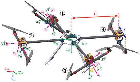
Figure 1.
Our platform and the defined coordinate system. We use different colors to indicate different frames, and the numbers represent the four propulsion units, respectively.
We now describe the four coordinate systems for our prototype:
- The world frame defined under the north–east–down convention.
- The body frame whose origin is at the center of mass. Here, points forward along arm 2, and is perpendicular to the fuselage plane, pointing downward.
- The origin of the static joint frame for the ith arm is located at the center of the revolute joint with its axis always remaining parallel to the axis.
- The rotatable joint frame for the ith arm , which can be obtained by rotating by degree.
A hierarchical approach is adopted to establish the system dynamics. The actuator dynamics are modeled first, followed by the formulation of the full-body translational and rotational dynamic models of the prototype.
2.1. Actuator Dynamics
Actuators consist of four propulsion units. The tilt angle of each unit is measured by the integrated IMU of each sub-controller.
We denote the attitude of the ith arm as in the world frame and as in the ith static joint frame , respectively. We denote the rotation from the ith static joint frame to the body frame as , and denote the rotation from the body frame to the world frame as . Let the angular velocity in be denoted as (the arm only rotates around -axis). Then, the dynamics for the ith arm can be written as
where ∧ transforms a vector into its associated skew-symmetric matrix, is the moment of inertia of the arm rotating around the joint, and is the torque generated by the two rotors on the ith arm.
Let the thrust of the ith arm be denoted by in the static joint frame and by in the body frame , respectively. Then, vanishes along the -axis, and it can be calculated by
Consequently, the control effective model for the ith arm becomes
where and are the thrusts generated by the ith arm’s rotors.
2.2. Platform Dynamics
Let the position of the body frame’s origin, , in the world frame be defined as . Let the attitude of the body frame relative to the world frame be defined as . Let the angular velocity in be denoted as .
Let the desired force be denoted as . Then, the translational dynamics can be written as
where is the acceleration of gravity in , and m is the total mass of the octocopter. In addition, the rotational dynamics of the platform can be written as
where is the positive definite inertia matrix and is the desired torque. For each arm, we write the position of the revolute joint center as
where h represents the distance between the origin of the static joint frame and the center of gravity along the vertical direction.
3. Nominal Controller
The hierarchical control is implemented using a cascaded controller. In particular, the position controller and attitude controller are designed first. Let be a new input, and let
The system is simplified into a series-integrated system through feedback linearization. A PID controller is designed for it:
where ∨ is the inverse operator of ∧, and and represent the desired position and attitude automatically generated by the remote controller, respectively. and are the positive definite diagonal gain matrices for the position loop and attitude loop, respectively. and are the controller gain matrices for the velocity loop and the angular velocity loop, respectively.
After finding , we substitute it back into (8) to solve for , and map to . Next, we expand (7) into matrix form:
where
Since the propulsion units of the prototype can only rotate around the arms, the generated thrust must be perpendicular to the arms. Therefore, this constraint can be formulated by applying a dimensionality reduction matrix :
where represents the reduced-dimension control effectiveness matrix. Thus, the solution to (11) can be represented by
Through (2), the obtained can be transformed into , which together with the current attitude in world frame can be used to calculate the desired attitude in the world frame. The rotation of the rotatable frame relative to the static frame can be determined using Rodrigues’ rotation formula:
where , , and . Here, denotes the normalization of .
Then, we transform into a world frame:
The calculated values of and are input into the sub-controller to compute the desired tilt angular velocity:
where is the attitude measured by the ith sub-controller, and is the positive definite diagonal gain matrices for the ith sub-controller. We use to compute the desired tilt angle :
where is the pitch angular velocity measured by the ith sub-controller. are the angular velocity gain matrices. By substituting into (3), the thrust for each pair of motors in the propulsion units can be computed as
Finally, the computed thrusts are converted into actual throttle signals using a thrust-to-throttle relationship, which can be obtained by the offline parameter identification test.
4. Geometric Allocation
For the free-hinged tiltrotor octocopter studied in this work, the primary goal of control allocation is to distribute the desired control forces and moments—generated by the high-level controller—to the individual actuators, namely the thrusts of the eight rotors and the tilt angles of the propulsion units. This allocation must satisfy the system’s physical constraints while maintaining acceptable computational complexity and optimizing control performance. Mathematically, the problem can be formulated as solving the actuator command vector through the control allocation mapping , where denotes the desired control input. In this context, represents the desired forces and torque, while corresponds to the tilt angles and thrust magnitudes of the propulsion units. Different control allocation strategies use different forms of the mapping , resulting in varying performance and computational requirements.
4.1. Force Decomposition Method
The FD method is characterized by low computational complexity and demonstrates reliable performance in practical applications. The core principle of this method is to decompose the thrust generated by each actuator along the coordinate axes of the body frame, thereby transforming the nonlinear control allocation problem into a linear system of equations. The required actuator thrusts and tilt angles are then obtained by solving the resulting linear system via the least-squares method.
Set the thrust generated by the ith propulsion unit be , and define . Then, the translational and rotational dynamics of the entire prototype can be written as follows:
where
Here, c and s denote the abbreviations of cos and sin, respectively. Let
For further simplification, we define and and construct the vector . Then, the control effectiveness model becomes:
where is a full row-rank control effectiveness matrix. Thus, can be obtained by taking the least-squares solution to this system.
Once is found, the desired thrust and tilt angle for each propulsion unit can be further calculated as follows:
The FD method offers low computational cost and supports real-time implementation at high control frequencies. However, it cannot directly incorporate constraints on (thrust) and (tilt angles). In addition, the FD method has limited capability in handling singularities and actuator saturation, which may compromise control accuracy and system stability under constrained conditions.
4.2. Nullspace-Based Method
To combining the advantages of the FD and QP methods, a nullspace-based control allocation method was proposed in [29]. In the FD method, the desired thrust vector is typically computed using the pseudoinverse, assuming . However, this expression only provides a particular solution and is not mathematically complete. The general solution should include a nullspace term and is given by:
where denotes the nullspace of , and is an arbitrary vector. In conventional FD methods, this is equivalent to assuming , meaning the nullspace is not used to further optimize the control allocation outcome. To incorporate this component, we perform a linearization of Equation (26) and derive a new equality constraint as follows:
where
At this point, is treated as an optimization variable in the QP problem and is introduced into the objective function for optimization. The objective function is:
where is the weighting matrix. The nullspace-based optimization problem is formulated into the standard form:
At this stage, (31) denotes the objective function, (32) corresponds to the inequality constraints that reflect actuator saturation limits, and (33) represents the equality constraints derived from the control effectiveness model. The optimal solution is solely determined by the nullspace matrix and can be calculated using the following expression:
The exact solution for the desired force is obtained by substituting the computed value of into Equation (26):
After obtaining , it is substituted into Equation (25) to compute the corresponding desired thrust and tilt angle for each propulsion unit.
Within the QP formulation based on the nullspace method, a new variable is introduced into both the objective function and the equality constraints. This variable represents the deviation between the dynamic model approximation and the least-squares solution , and is optimized to correct this mismatch.
Due to the properties of the nullspace matrix, for any , the expression remains a valid solution for . This allows to be computed at high frequency, while is updated at a lower frequency and added as a compensatory term. This strategy combines the real-time efficiency of the FD method and the constraint-handling capability of the QP framework, resulting in improved actuator saturation management, control accuracy, and robustness.
5. Control Allocation Method Considering Thrust Balance
In the previous section, actuator saturation was addressed by integrating the nullspace method with both the FD and QP approaches, resulting in a QP-based control allocation framework. An optimization variable is introduced, defined as , where and represent the incremental changes in thrust and tilt angle, respectively. However, since the method simultaneously optimizes both variables, it may lead to unbalanced thrust allocation in practical applications. In some cases, thrust is unnecessarily constrained in order to maintain small tilt angles, which reduces the method’s effectiveness in mitigating actuator saturation.
To address this limitation, a tailored control allocation strategy is proposed based on the specific characteristics of the freely hinged tilt-rotor UAV. This type of platform can maintain stable flight performance even with large tilt angles of the propulsion units, making strict constraints on unnecessary in practical scenarios. Based on this observation, the optimization objective is reformulated to focus solely on , thereby enhancing the coordination and flexibility of thrust allocation.
Our platform is equipped with eight rotors and exhibits an overall thrust-to-weight ratio exceeding 2, enabling high-acceleration maneuvers. As a result, the main challenge in control allocation lies in effectively distributing thrust among the eight rotors, ensuring that each propeller operates within safe speed limits while fully using the available thrust to maximize overall flight performance.
To address this challenge, a min–max-based control allocation strategy is proposed. The key idea is to minimize the maximum individual thrust among all rotors, thereby achieving a more balanced thrust distribution. This approach promotes full utilization of actuator capabilities, prevents saturation caused by thrust imbalances, and enhances the platform’s maneuverability within safe operating bounds. Furthermore, by incorporating nullspace-based correction in conjunction with the FD method, the proposed strategy improves both real-time performance and overall system stability.
5.1. Min–Max-Based Control Allocation Strategy
To construct the new optimization problem, the actuator control variable and the state matrix are retained from the nullspace method introduced in Section 4.2:
At this stage, the control allocation task is formulated as the following optimization problem:
Here, denotes an m-by-n zero matrix. The objective function (37) seeks a solution that balances the thrusts of the propulsion unit in an evenly distributed manner. The inequality constraint (38) imposes limits on the thrust magnitude, while the equality constraint (39) remains based on the linearized control effectiveness model, which is identical to Equation (33). However, the objective function is nonlinear and non-smooth, which introduces difficulties for conventional optimization algorithms. Therefore, it is necessary to reformulate this problem as a linear optimization task to facilitate computational efficiency and solvability.
To linearize the objective function, we introduce an auxiliary variable t and derive an equivalent reformulation of the objective function (37):
We also notice the following equivalent relation:
We define:
By substituting Equations (41) and (40) into (37), we obtain the following linear optimization problem:
Through the linearization process described above, the original nonlinear min–max optimization problem is transformed into a standard linear programming (LP) formulation, which can be efficiently solved using well-established linear optimization solvers. This transformation significantly reduces computational complexity while enhancing solution stability and numerical convergence. For practical implementation, the active-set solver [30] is employed, as it is well suited for small-scale, highly constrained linear and quadratic programming problems. Its ability to handle constraint activation and deactivation efficiently allows the min–max problem to be solved in real time.
To further improve real-time performance, the min–max method is integrated with the FD method via nullspace mapping. Specifically, the min–max algorithm is used to compute the compensation term in Equation (26). In practical, the FD method operates at high frequency to provide fast control response, while the min–max component runs at a lower frequency to optimize the compensation term, thereby correcting thrust imbalances and preventing actuator saturation. This integration leverages the computational efficiency of the FD method alongside the thrust-balancing capability of the min–max strategy.
The proposed control allocation strategy significantly improves thrust distribution balance, enabling full use of the octocopter’s propulsion resources and maximizing its maneuverability. At the same time, it effectively prevents actuator saturation, ensuring all actuators remain within safe operating limits and avoiding performance degradation. Moreover, the strategy provides high real-time performance and strong robustness, making it well suited for dynamic environments and offering reliable support for attitude control and trajectory tracking in freely hinged tilt-rotor UAVs.
5.2. Control Allocation Strategy Based on Simple Neural Network and Min–Max Method
In the previous section, we proposed a control allocation method specifically designed for a freely hinged tilt-rotor octocopter UAV—namely, a min–max-based control allocation strategy. This method exhibited strong performance in simulation tests, effectively balancing thrust distribution and mitigating actuator saturation while maintaining high real-time capability and system stability. However, such performance relies on the availability of sufficient computational resources. In practical UAV platforms, where onboard computational capacity is often limited, solving optimization problems in real time imposes significant computational overhead. This can degrade control performance, slow system response, and ultimately fail to meet the stringent real-time requirements of high-frequency control loops.
To address this challenge and enable the application of the min–max method in embedded onboard environments, we further enhance the strategy by integrating a computationally efficient neural network into the control allocation framework. The core idea is to replace the online optimization process—originally used to compute the compensation term —with a neural network approximation. Specifically, offline training is performed on the ground, during which the neural network learns the mapping from the desired control input to the optimal compensation term . Once trained, the network is deployed onboard, allowing the UAV to directly infer in real time, thereby eliminating the computational burden associated with online optimization.
This strategy significantly reduces computational load and enhances the real-time performance of control allocation, while maintaining high control accuracy. As a result, it can be directly implemented on the flight control board without requiring additional onboard computing hardware. This reduces system load, extends flight duration and operational range, and increases available payload capacity. Ultimately, it enhances the UAV’s adaptability and practical utility in complex mission scenarios.
- Target Mapping for ApproximationThe min–max-based control allocation optimization problem is formulated in Section 5.1, with the objective function, inequality constraints, and equality constraints given by Equations (43)–(45), respectively. Accordingly, the neural network is trained to approximate the mapping from the desired control input to the optimal compensation term :where denotes the neural network and represents its trainable parameters.
- Generating the Training DatasetA control allocation training dataset is constructed to train the neural network, where denotes the control input vector representing the desired forces and torques along the three axes, and is the optimal compensation term used to correct the FD result via nullspace projection. To generate the dataset, simulated flight experiments are conducted using the MATLAB R2023b Simscape platform. During each simulation, the high-level controller outputs a sequence of desired control inputs , which are passed to an active-set solver to solve the min–max linear programming problem and obtain the corresponding optimal compensation term .
- Network Architecture DesignA fully connected feedforward neural network (multi-layer perceptron, MLP) is adopted, as it is well suited for small-scale regression tasks involving low-dimensional control inputs. The input layer contains six neurons, corresponding to the control input . The network consists of two hidden layers with 20 and 10 neurons, respectively, both fully connected. The output layer consists of two neurons, representing the elements of the compensation vector . The overall architecture of the designed neural network is illustrated in Figure 2.
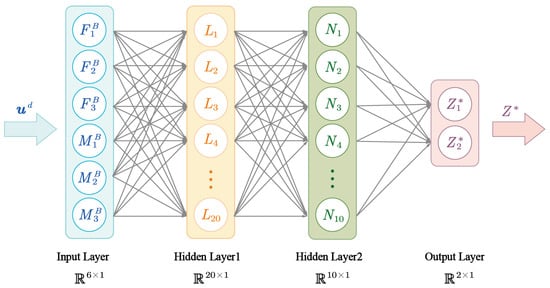 Figure 2. Schematic diagram of the neural network architecture. We use different colors to indicate different neural network layers, and the asterisk (*) indicates the output.
 - Neural Network TrainingThe neural network is trained using the Levenberg–Marquardt (LM) algorithm, which combines the advantages of gradient descent and Newton’s method to achieve fast convergence and improved numerical stability. The algorithm adaptively adjusts the step size during optimization: it provides strong global search capability when far from the optimum and accelerates convergence as the solution is approached. The LM algorithm is particularly effective for training small- to medium-scale feedforward neural networks, such as the one used in this study. Compared to conventional gradient descent methods, LM converges more rapidly while avoiding the numerical instability associated with inverting the Hessian matrix in classical Newton-based approaches.During training, the number of epochs is set to 500, the convergence tolerance is defined as , and the learning rate is set to 0.01.The LM-based training process ensures efficient and robust convergence of the neural network, effectively avoiding numerical instability and enabling reliable learning of the compensation mapping.
We have now completed the design of the control allocation strategy based on a lightweight neural network combined with the min–max method. By replacing the computationally intensive online optimization with a pre-trained neural network, the proposed approach significantly improves computational efficiency and reduces the computational load on onboard processors. This enhancement in real-time capability enables direct deployment on the flight controller without the need for additional hardware. Moreover, the strategy maintains control accuracy and system stability, thereby improving the adaptability of the control system without compromising optimization performance.
In the following sections, simulations and real-world flight experiments will be conducted on the octocopter platform to validate the effectiveness of the proposed method.
6. Simulation and Experiment
6.1. Simulation
To validate the proposed control allocation strategy, a series of comparative simulations were conducted using the Simscape module in MATLAB R2023b Simulink. Simscape provides a physics-based simulation environment capable of modeling multi-domain physical systems with high fidelity. Its ability to capture the nonlinear dynamics and interactions between mechanical, electrical, and control components makes it well suited for the high-precision simulation of aerial vehicle dynamics. Consequently, simulation results obtained in this platform are considered reliable for pre-deployment validation of control strategies.
In this study, four control allocation methods mentioned in Section 4 were evaluated: the FD method, the nullspace method, the min–max method, and the min–max neural network method. To compare their performance, a trapezoidal reference command with a peak amplitude of was injected into the pitch channel. This command induces a large-angle rotation around the pitch axis, followed by 12 s of steady hover. This scenario not only examines the system’s stability and control precision under large-angle conditions, but also provides a stringent test for actuator allocation, as the propulsion units are prone to saturation at such pitch angles. It thus serves as a robust benchmark for evaluating the effectiveness and fault tolerance of the proposed min–max neural network-based control allocation strategy.
The corresponding simulation results are presented in Figure 3 and Figure 4. Figure 3 illustrates the responses of the FD and nullspace methods, denoted by labels “F” and “N”, respectively. Figure 4 shows the performance of the min–max and min–max neural network methods, denoted by “M” and “MN”. The video of the simulations is available at https://easylink.cc/mxg1f0 (accessed on 27 April 2025).
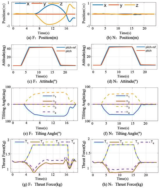
Figure 3.
Simulation results of the FD method and nullspace method. This figure illustrates the responses of the FD and nullspace methods, denoted by labels “F” and “N”, respectively. Figure 4 shows the performance of the min–max and min–max neural network methods, denoted by “M” and “MN”.
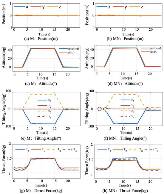
Figure 4.
Simulation results of the min–max method and min–max neural network method. This figure shows the performance of the min–max and min–max neural network methods, denoted by “M” and “MN”.
As observed from the simulation results, both the proposed min–max method and the nullspace method successfully completed the hover task, while the FD method exhibited a clear divergence trend around the 6 s mark.During the increasing tilt phase, the thrust of Propulsion Units 1 and 3 in the FD method continuously rose and eventually reached the saturation limit, which was set to 1.7 kg in this simulation. In contrast, the thrust of Units 2 and 4 remained low and were not effectively used.
Since the FD method handles actuator saturation through direct truncation without redistributing the load via tilt angle adjustments, it fails to achieve effective redundancy management. In this scenario, the maximum tilt angle remained below , which was insufficient to maintain stable control, ultimately leading to severe divergence in the position channel. In our ideal Simscape environment—where no aerodynamic disturbances or collisions occur beyond rotor thrust—position diverges first, and attitude drift takes longer to develop, so attitude remains apparently stable within the simulated timeframe.
In contrast, the nullspace control allocation method demonstrates a certain degree of effectiveness in managing actuator saturation. When Propulsion Units 1 and 3 approached saturation, the controller dynamically adjusted the corresponding tilt angles (Figure 3f), thereby enabling the system to utilize the remaining thrust capacity of Units 2 and 4. This allowed the UAV to maintain overall stability and exhibit reasonably good hovering performance.
However, this approach remains inherently inefficient in terms of resource allocation. Despite Units 1 and 3 nearing their thrust limits, the nullspace method does not actively reallocate the load to Units 2 and 4 in a proactive manner. As a result, if the commanded attitude angle were further increased, Units 1 and 3 would be unable to generate additional thrust, and the UAV would ultimately fail to maintain its orientation.
Furthermore, as demonstrated in the simulation results, although both the QP-based and nullspace-based methods are capable of mitigating actuator saturation to some extent, their effectiveness primarily relies on reactive redistribution when certain actuators approach their saturation limits. This reactive behavior fails to fully exploit the capabilities of all actuators throughout the control process. As a result, we observe that two arms of the UAV frequently operate near maximum thrust, while the other two remain at nearly half thrust. This leads to a flight condition that is persistently close to saturation, leaving minimal control margin for disturbance rejection or trajectory correction.
In contrast, our proposed method based on the min–max objective achieves a more balanced thrust distribution, where all four actuators increase their output simultaneously. Upon reaching the target, all four thrusts approach saturation nearly at the same time, indicating that actuator usage is fully optimized without prematurely exhausting any single actuator’s capability. This balanced utilization ensures sufficient control authority is retained during flight and clearly demonstrates the advantage of the min–max objective for our specific UAV configuration. This is the main reason we deliberately chose to incorporate the min–max formulation into our control allocation strategy, rather than adopting alternative cost functions that do not inherently encourage uniform actuator usage.
In comparison, the min–max method demonstrates superior rationality and efficiency in actuator resource utilization. As shown in Figure 4a, the position response under this method remains smooth and stable, with no signs of divergence. By optimizing the maximum thrust across all actuators, the method ensures a more balanced distribution of thrust among the four propulsion units. During the progressive increase in tilt angles, all four thrust outputs grow in a coordinated manner and remain well below the saturation limit throughout the maneuver. Simultaneously, the min–max method makes full use of the available tilt angle range, with the maximum tilt reaching up to 90°. This enables the UAV to maintain both position and attitude stability even during large-angle operations.
This characteristic is particularly well suited for passive-hinged tilt-rotor platforms, where the tilt angle is theoretically unbounded, while the available thrust is inherently limited.
The neural network-based min–max method was trained offline using sampled data from the original min–max optimization strategy. Its design objective is to closely approximate the control behavior of the original algorithm. As illustrated in Figure 4, the neural approximation exhibits highly consistent performance with the original min–max method in terms of position tracking, attitude regulation, thrust distribution, and tilt angle response. Minor discrepancies are observed in the precision of thrust allocation, where the thrusts of certain propulsion units are slightly less balanced compared to those obtained from the original optimization algorithm. Nevertheless, as the outputs of the neural network still reside within the feasible solution space defined by the nullspace mapping, these differences have negligible impact on the overall control performance.
All timing data in Table 1 were obtained by running each allocation routine in MATLAB R2023b on a desktop PC (Intel Core i7, 8 cores, 64 GB RAM, 3.5 GHz). From Table 1 we see that the full min–max method incurs the highest cost (9.43 ms per iteration), followed by the nullspace correction (5.22 ms). The FD algorithm is extremely light, at under 0.1 ms, but it cannot handle saturation. The MN approach—the neural-network approximation of the min–max solution—requires only 0.12 ms per iteration, nearly matching the speed of FD while still enforcing actuator constraints. In other words, MN achieves almost FD-level computational efficiency, yet provides the thrust-balancing benefits of min–max optimization. This makes MN ideally suited for high-rate, onboard deployment on resource-limited flight controllers.

Table 1.
Average time per iteration of methods in simulation.
6.2. Experiment
To validate the practical feasibility and performance of the proposed control allocation strategy based on min–max optimization and a lightweight neural network, the algorithm was implemented on the onboard flight control board. A real-world flight experiment involving large-angle attitude hovering was conducted, as illustrated in Figure 5. The video of the experiment is available at: https://easylink.cc/9rdwjh (accessed on 27 April 2025).
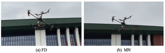
Figure 5.
The comparative experiment is conducted to validate the controller performance in real platform.
In the experiment, a trapezoidal attitude command with a peak amplitude of and a duration of 20 s was applied to the roll channel, requiring the UAV to maintain a steady roll attitude for an extended period. This task evaluates not only the controller’s stability and accuracy under large-angle conditions but also the efficiency of actuator allocation and its capability to handle saturation near operational limits.
To ensure flight safety and protect the hardware, the maximum thrust for each motor was conservatively limited to 1.4 kg—below the design limit of 1.7 kg—to prevent thermal overload or potential damage from sustained high-power operation. This constraint increases the safety margin of the flight test. In practice, we chose instead of the used in simulation because, under the 1.4 kg thrust cap, commands beyond already risk pushing the motors into saturation and overstressing the system. This constraint increases the safety margin of the flight test.
Due to the relatively high computational demands of both the nullspace method and the original min–max optimization algorithm, neither could be executed in real time on the onboard flight controller. Therefore, only the FD method and the neural network-based min–max approximation were selected for hardware deployment, allowing for a direct comparison of control performance. The experimental results are presented in Figure 6, where the left column shows the flight responses using the FD method, and the right column corresponds to those obtained with the min–max neural network approach. Notable differences are observed between the two methods across various metrics, including position tracking, attitude regulation, tilt angle evolution, and thrust distribution.
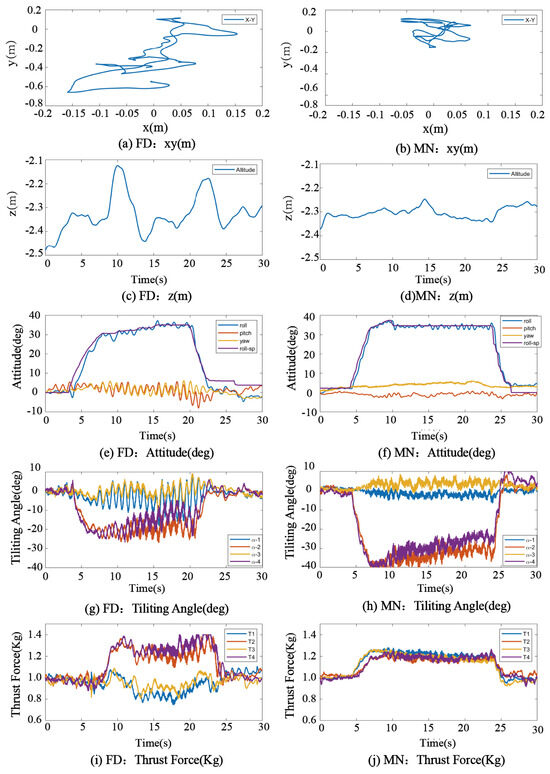
Figure 6.
The comparative experiment is conducted to validate the controller performance in a real platform. The left column shows the flight responses using the FD method, and the right column corresponds to those obtained with the min–max neural network approach.
During the initial phase of increasing roll angles, both control methods exhibited satisfactory performance in position and attitude tracking, with the system responding stably to the input commands. However, as the roll angle continued to increase, the FD method gradually revealed its limitations in actuator allocation. As shown in Figure 6i, between 20 and 25 s, the thrusts of Propulsion Units 2 and 4 steadily increased and eventually reached the saturation limit of 1.4 kg, resulting in hard truncation. This truncation disrupted the continuity and adjustability of thrust distribution, leading to pronounced oscillations in the attitude response (Figure 6e) accompanied by evident thrust fluctuations. Specifically, since Units 2 and 4 are primarily responsible for generating roll torque, their saturation severely compromised the system’s lateral control authority along the y-axis, resulting in significant position drift in that direction—substantially exceeding the error along the x-axis. Moreover, due to the truncated thrust output, the available vertical force component also dropped sharply, causing strong oscillations in the altitude channel.
At the same time, the tilt angle allocation under the FD method appeared conservative. As shown in Figure 6g, the maximum tilt angle was limited to approximately −20°, failing to exploit the system’s available redundancy to alleviate saturation. This caused Units 2 and 4 to carry most of the load, resulting in highly uneven thrust distribution.
In contrast, the proposed min–max neural network control method demonstrated superior resource allocation and control robustness. As shown in Figure 6b,d, both position and attitude errors remained consistently low throughout the entire roll angle increase phase. The system maintained stable operation without any thrust saturation. Figure 6j indicates that the thrust was evenly distributed across all four propulsion units, with no signs of local overload. The tilt capability of the actuators was effectively used, with the maximum tilt angle reaching approximately −40°, thereby fully exploiting the system’s actuation redundancy. This ensured sufficient lateral thrust along the y-axis to maintain balance, while the vertical component of the total thrust remained adequate for stable altitude control. As a result, stable tracking was achieved in all three translational axes (x, y, and z), along with consistent and accurate attitude control throughout the maneuver.
In summary, the min–max neural network-based method outperforms the traditional FD approach in terms of control accuracy, attitude stability, thrust allocation balance, and resistance to actuator saturation. During angle-hover flight tasks, the FD method is prone to thrust imbalance, attitude oscillations, and even position instability due to its neglect of saturation constraints. By contrast, the proposed min–max neural network method effectively addresses these issues through an optimization-driven objective and an efficient neural approximation. It maintains high control performance while significantly reducing online computational demands, making it more suitable for practical deployment and real-time application on embedded flight control platforms.
To quantitatively evaluate the control accuracy of different allocation strategies in real-world flight experiments, this study reports the root mean square error (RMSE) in both position and attitude channels, as well as the maximum attitude deviation during the attitude-holding task. The results for the FD method and the min–max neural network method are summarized in Table 2.
Table 2.
Comparison of position and attitude control errors between the FD method and min–max neural network method.
In terms of position RMSE, the min–max neural network method outperforms the FD method across all three axes, with the most notable improvement observed along the y-axis—where the error is reduced from 0.2625 m to 0.069 m. This aligns closely with the improved trajectory convergence observed in Figure 6a,b. Overall, the min–max approach demonstrates higher robustness and faster convergence in spatial accuracy control. For attitude RMSE, the min–max method also shows consistent improvements. The roll and pitch errors are reduced from and to and , respectively, while the yaw error decreases from to . These results indicate enhanced stability across all three attitude channels. The findings confirm that the proposed min–max strategy can effectively handle actuator nonlinearities and coupling disturbances under complex attitude conditions, resulting in significantly improved attitude-holding precision.
Furthermore, in terms of maximum attitude deviation, the FD method exhibits significant peak errors of , , and in the roll, pitch, and yaw channels, respectively. These large deviations indicate transient control imbalance and substantial divergence from the target attitude during dynamic maneuvers. In contrast, under the same conditions, the min–max neural network method effectively reduces the maximum errors to , , and in the corresponding channels. This demonstrates a strong suppression of transient overshoot and a significant enhancement in the dynamic responsiveness and control safety of the attitude channels during angle-hover flight tasks.
In summary, the min–max neural network control strategy outperforms the conventional FD method in terms of control accuracy, dynamic robustness, and attitude convergence, demonstrating greater practical applicability.
7. Conclusions
This paper introduces a simple control-allocation method for servo-free, passive-hinge tilt-rotor octocopters. It merges a nullspace FD formula with min–max optimization. A small neural network, trained offline, replaces the heavy optimization online. This keeps computations fast and avoids actuator saturation. In simulations, it gives smoother flights, balanced thrust, and better handling near singularities. Flight tests at 35° roll confirm stable, accurate attitude tracking. The network version also cuts RMSE and peak errors versus standard FD. It runs directly on limited hardware without extra components. Adapting the method to other UAVs only requires updating the effectiveness matrix and retraining the network.
Author Contributions
Conceptualization, K.L. (Kaixin Li); Funding acquisition, K.L. (Kun Liu); Methodology, K.L. (Kaixin Li) and K.L. (Kun Liu); Software, M.L.; Supervision, K.L. (Kun Liu); Validation, X.L.; Visualization, K.L. (Kaixin Li) and M.L.; Writing—original draft, K.L. (Kaixin Li); Writing—review and editing, M.L. and X.Y. All authors have read and agreed to the published version of the manuscript.
Funding
This research received no external funding.
Data Availability Statement
Data are unavailable due to privacy or ethical restrictions.
Acknowledgments
Thanks to Zijie Qin and all the members of the Aircraft Group in the FM Team at Sun Yat-sen University for their support and assistance.
Conflicts of Interest
The authors declare no conflicts of interest.
References
- Al-Dhaifallah, M.; Al-Qahtani, F.M.; Elferik, S.; Saif, A.W.A. Quadrotor robust fractional-order sliding mode control in unmanned aerial vehicles for eliminating external disturbances. Aerospace 2023, 10, 665. [Google Scholar] [CrossRef]
- Delavarpour, N.; Koparan, C.; Nowatzki, J.; Bajwa, S.; Sun, X. A technical study on UAV characteristics for precision agriculture applications and associated practical challenges. Remote Sens. 2021, 13, 1204. [Google Scholar] [CrossRef]
- Munawar, H.S.; Hammad, A.W.; Waller, S.T.; Thaheem, M.J.; Shrestha, A. An integrated approach for post-disaster flood management via the use of cutting-edge technologies and UAVs: A review. Sustainability 2021, 13, 7925. [Google Scholar] [CrossRef]
- Wang, G.; Chen, Y.; An, P.; Hong, H.; Hu, J.; Huang, T. UAV-YOLOv8: A small-object-detection model based on improved YOLOv8 for UAV aerial photography scenarios. Sensors 2023, 23, 7190. [Google Scholar] [CrossRef]
- Ding, C.; Lu, L.; Wang, C.; Ding, C. Design, sensing, and control of a novel UAV platform for aerial drilling and screwing. IEEE Robot. Autom. Lett. 2021, 6, 3176–3183. [Google Scholar] [CrossRef]
- Li, Z.; Yang, Y.; Yu, X.; Liu, C.; Kaynak, O.; Gao, H. Fixed-Time Control of a Novel Thrust-Vectoring Aerial Manipulator via High-Order Fully Actuated System Approach. IEEE/ASME Trans. Mechatron. 2024, 30, 1084–1095. [Google Scholar]
- Kamel, M.; Verling, S.; Elkhatib, O.; Sprecher, C.; Wulkop, P.; Taylor, Z.; Siegwart, R.; Gilitschenski, I. Voliro: An Omnidirectional Hexacopter with Tiltable Rotors. arXiv 2018, arXiv:1801.04581. [Google Scholar]
- Allenspach, M.; Bodie, K.; Brunner, M.; Rinsoz, L.; Taylor, Z.; Kamel, M.; Siegwart, R.; Nieto, J. Design and optimal control of a tiltrotor micro-aerial vehicle for efficient omnidirectional flight. Int. J. Robot. Res. 2020, 39, 1305–1325. [Google Scholar] [CrossRef]
- Abara, D.N. Modelling, Control and Construction of Tricopter Unmanned Aerial Vehicles; The University of Manchester: Manchester, UK, 2022. [Google Scholar]
- Zhou, H.; Li, B.; Wang, D.; Ma, L. Design, Modeling and Control of a Novel Over-Actuated Hexacopter with Tiltable Rotors. In Proceedings of the 2021 IEEE 16th Conference on Industrial Electronics and Applications (ICIEA), Chengdu, China, 1–4 August 2021; pp. 1079–1084. [Google Scholar] [CrossRef]
- Bodie, K.; Brunner, M.; Pantic, M.; Walser, S.; Pfändler, P.; Angst, U.; Siegwart, R.; Nieto, J. Active interaction force control for contact-based inspection with a fully actuated aerial vehicle. IEEE Trans. Robot. 2020, 37, 709–722. [Google Scholar] [CrossRef]
- Santos, M.; Honório, L.; Moreira, A.P.G.M.; Silva, M.; Vidal, V.F. Fast real-time control allocation applied to over-actuated quadrotor tilt-rotor. J. Intell. Robot. Syst. 2021, 102, 65. [Google Scholar] [CrossRef]
- Lee, H.; Yu, B.; Tirtawardhana, C.; Kim, C.; Jeong, M.; Hu, S.; Myung, H. CAROS-Q: Climbing aerial robot system adopting rotor offset with a quasi-decoupling controller. IEEE Robot. Autom. Lett. 2021, 6, 8490–8497. [Google Scholar] [CrossRef]
- Lv, Z.Y.; Wu, Y.; Zhao, Q.; Sun, X.M. Design and control of a novel coaxial tilt-rotor UAV. IEEE Trans. Ind. Electron. 2021, 69, 3810–3821. [Google Scholar] [CrossRef]
- Lv, Z.; Sun, Y.; Li, S.; Wu, Y.; Sun, X.M. Coaxial Tilt-Rotor UAV: Fixed-time Control, Mixer, and Flight Test. IEEE Trans. Intell. Veh. 2024, 1–12. [Google Scholar] [CrossRef]
- Wang, S.; Ma, L.; Li, B.; Zhang, K. Architecture design and flight control of a novel octopus shaped multirotor vehicle. IEEE Robot. Autom. Lett. 2021, 7, 311–317. [Google Scholar] [CrossRef]
- Pi, C.H.; Ruan, L.; Yu, P.; Su, Y.; Cheng, S.; Tsao, T.C. A simple six degree-of-freedom aerial vehicle built on quadcopters. In Proceedings of the 2021 IEEE Conference on Control Technology and Applications (CCTA), San Diego, CA, USA, 9–11 August 2021; pp. 329–334. [Google Scholar]
- Qin, Z.; Wei, J.; Cao, M.; Chen, B.; Li, K.; Liu, K. Design and flight control of a novel tilt-rotor octocopter using passive hinges. IEEE Robot. Autom. Lett. 2023, 9, 199–206. [Google Scholar] [CrossRef]
- Qin, Z.; Wei, J.; Liu, K.; Wang, C.; Li, X.; Yu, X. Improving the Controller Performance of a Tilt-Rotor Octocopter by Compensating for the Tilt Angle’s Dynamics. IEEE Robot. Autom. Lett. 2024, 9, 11010–11017. [Google Scholar] [CrossRef]
- Su, Y.; Jiao, Z.; Zhang, Z.; Zhang, J.; Li, H.; Wang, M.; Liu, H. Flight structure optimization of modular reconfigurable uavs. In Proceedings of the 2024 IEEE/RSJ International Conference on Intelligent Robots and Systems (IROS), Abu Dhabi, United Arab Emirates, 14–18 October 2024; pp. 4556–4562. [Google Scholar]
- Kamel, M.; Verling, S.; Elkhatib, O.; Sprecher, C.; Wulkop, P.; Taylor, Z.; Siegwart, R.; Gilitschenski, I. The voliro omniorientational hexacopter: An agile and maneuverable tiltable-rotor aerial vehicle. IEEE Robot. Autom. Mag. 2018, 25, 34–44. [Google Scholar] [CrossRef]
- Su, Y. Compensation and Control Allocation with Input Saturation Limits and Rotor Faults for Multi-Rotor Copters with Redundant Actuations. Ph.D Thesis, Univercity of California, Los Angeles, CA, USA, 2021. [Google Scholar]
- Johansen, T.; Fossen, T.; Berge, S. Constrained nonlinear control allocation with singularity avoidance using sequential quadratic programming. IEEE Trans. Control. Syst. Technol. 2004, 12, 211–216. [Google Scholar] [CrossRef]
- Zhang, Z.; Chen, T.; Zheng, L.; Luo, Y. A quadratic programming based neural dynamic controller and its application to UAVs for time-varying tasks. IEEE Trans. Veh. Technol. 2021, 70, 6415–6426. [Google Scholar] [CrossRef]
- Zhang, R.; Zhang, Y.; Tang, R.; Zhao, H.; Xiao, Q.; Wang, C. A joint UAV trajectory, user association, and beamforming design strategy for multi-UAV assisted ISAC systems. IEEE Internet Things J. 2024, 11, 29360–29374. [Google Scholar] [CrossRef]
- Yang, Y.; Yu, X.; Li, Z.; Basin, M.V. A new overactuated multirotor: Prototype design, dynamics modeling, and control. IEEE Trans. Ind. Electron. 2023, 71, 9449–9459. [Google Scholar] [CrossRef]
- Su, Y.; Zhang, J.; Jiao, Z.; Li, H.; Wang, M.; Liu, H. Real-time dynamic-consistent motion planning for over-actuated uavs. In Proceedings of the 2024 IEEE International Conference on Robotics and Automation (ICRA), Yokohama, Japan, 13–17 May 2024; pp. 11789–11795. [Google Scholar]
- Zhang, Z.; Li, J.; Wang, J. Sequential convex programming for nonlinear optimal control problems in UAV path planning. Aerosp. Sci. Technol. 2018, 76, 280–290. [Google Scholar] [CrossRef]
- Su, Y.; Yu, P.; Gerber, M.J.; Ruan, L.; Tsao, T.C. Nullspace-Based Control Allocation of Overactuated UAV Platforms. IEEE Robot. Autom. Lett. 2021, 6, 8094–8101. [Google Scholar] [CrossRef]
- Ferreau, H.J.; Kirches, C.; Potschka, A.; Bock, H.G.; Diehl, M. qpOASES: A parametric active-set algorithm for quadratic programming. Math. Program. Comput. 2014, 6, 327–363. [Google Scholar] [CrossRef]
Disclaimer/Publisher’s Note: The statements, opinions and data contained in all publications are solely those of the individual author(s) and contributor(s) and not of MDPI and/or the editor(s). MDPI and/or the editor(s) disclaim responsibility for any injury to people or property resulting from any ideas, methods, instructions or products referred to in the content. |
© 2025 by the authors. Licensee MDPI, Basel, Switzerland. This article is an open access article distributed under the terms and conditions of the Creative Commons Attribution (CC BY) license (https://creativecommons.org/licenses/by/4.0/).