Urban Wind Field Effects on the Flight Dynamics of Fixed-Wing Drones

Abstract

Urban wind, and particularly turbulence present in the roughness zone near structures, poses a critical challenge for next-generation drones. Complex flow patterns induced by large buildings produce significant disturbances that the vehicle must reject at low altitudes. Traditional turbulence models, such as the von Kármán model, underestimate these localized effects, compromising flight safety. To address this gap, we integrate high-resolution time and spatially varying urban wind fields from Large Eddy Simulations into a flight dynamics simulation framework using vehicle plant models based on configuration geometry and commonly deployed Ardupilot control laws, enabling a detailed analysis of drone responses in urban environments. Our results reveal that high-risk flight zones can be systematically identified by correlating drone response metrics with the spatial distribution of Turbulent Kinetic Energy (TKE). Notably, maximum g-loads coincide with abrupt TKE transitions, underscoring the critical impact of even short-lived wind fluctuations. By coupling advanced computational fluid dynamics with a real-time vehicle dynamics model, this work establishes a foundational methodology for designing safer and more reliable advanced air mobility platforms in complex urban airspaces. This work distinguishes itself from the existing literature by incorporating an efficient vortex lattice aerodynamic solver that supports arbitrary fixed-wing drone platforms through the simple specification of planform geometry and mass properties, and operating full-flights throughout a time and spatially varying urban wind field. This framework enables a robust assessment of stability and control for a wide range of fixed-wing drone platforms operating in urban environments, with delivery drones serving as a representative and practical use case.

1. Introduction

The Advanced Aerial Mobility (AAM) concept envisions a significant expansion in how aviation impacts daily life. This includes short-range passenger transportation around major metropolitan areas using electrified vertical takeoff and landing air taxis, the regional transportation of people and cargo via electrified aircraft, and the widespread use of small drones for urban deliveries [1]. Due to their small size, relatively slow flight speeds compared to wind speeds, and light wing loading, which amplifies turbulence effects [2], drones are more susceptible to flow features in the urban environment than heavier, faster-moving, manned aircraft [3]. Therefore, small fixed-wing drones are the focus of the current work. Many technological challenges must be overcome before vast quantities of drones are deployed in urban areas [4]. However, the economic appeal of improving logistics and efficiency in last-mile deliveries is strong [5]. To some extent, this future is already here: major companies have recently navigated technical and regulatory challenges within the United States to meet the growing demands of e-commerce. They are using drones for small parcel deliveries in limited suburban areas [6], marking an early step in the road map toward widespread drone delivery in major cities worldwide.

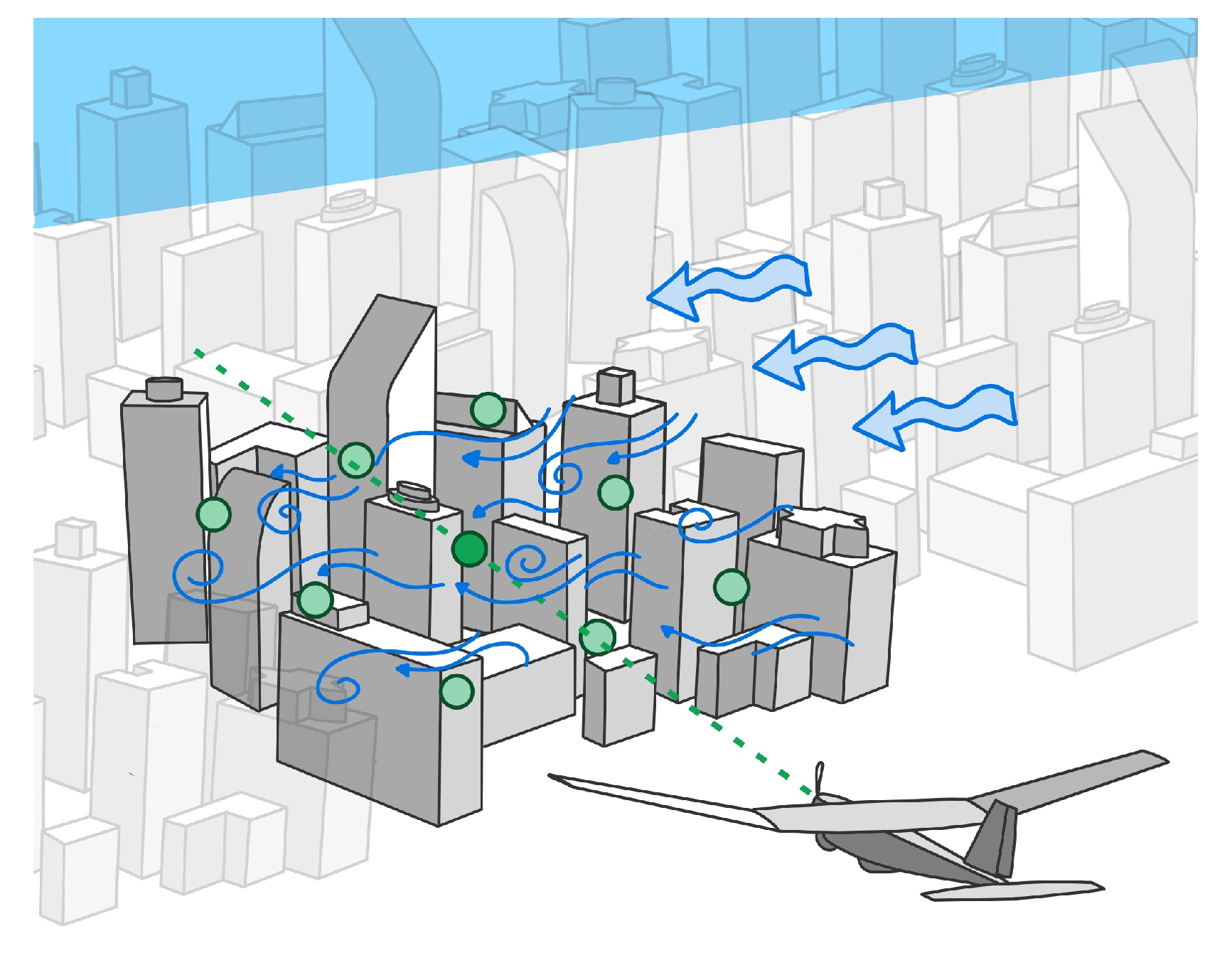
Urban environments present unique challenges, characterized by complex wind patterns resulting from buildings and varying terrain, which result in rapid changes in wind velocity and direction, which are especially impactful for drone platforms [7]. Safe vehicle-operating envelopes are often explored using flight dynamics simulation frameworks, designed to understand vehicle dynamics and control system responses. In simulation environments, it is common to specify turbulence intensity using von Kármán or Dryden models, as per the guidance in military specifications and civil aviation standards such as Refs. [8,9], respectively. Spectral turbulence model intensity ($\sigma$) scales, as a function of altitude based on atmospheric model expectations, and length scale (L) values are recommended, which further modify the impact of turbulence on the drone. Favorable comparison data are available to show that such atmospheric models replicate the turbulence seen in open-air environments, such as the data presented in Ref. [10]. However, many key assumptions of common Dryden and von Kármán models are violated within urban environments, in which large structures strongly influence the flow [11].

Within the roughness zone near structures, turbulent airflow impacts a drones’s navigational accuracy and creates demands on its flight control system to reject these disturbances [12]. Understanding how delivery drones interact with these dynamic wind conditions is essential for ensuring safe and efficient operations. The research community has developed atmospheric models using computational means; for example, Galeway et al. [13] used a Reynolds Average Navier–Stokes (RANS) approach to capture the urban wind effects. The atmospheric modeling community has moved more recently towards using higher-fidelity approaches, such as Large-Eddy Simulation (LES) for urban wind models, which offer more accurate and reliable results [14,15].

There are few studies in which realistic urban turbulence is coupled with a dynamic model of a drone navigating a cityscape. One example is the work by Mohamed et al. [16], using a two-dimensional frozen turbulent field (i.e., no temporal variation). Another example is provided by the work of Galway et al. [13], in which the authors rely on a preexisting aerodynamic model of the Aerosonde platform. A comprehensive simulation environment is outlined by Cybyk et al. [17], which has many of the same features as the simulation environment demonstrated herein.

This work expands the scope of previous studies in many ways. We developed a comprehensive urban wind model for a notional cityscape using high-fidelity LES CFD and represent the time- and spatially varying winds for several separate inflow azimuth cases. We present wind data for each case, including the turbulent kinetic energy (TKE) atmospheric metric for the resulting wind fields. For comparison, we also present a case in which the city is absent, based on the same precursor flow simulation used to generate an atmospheric boundary layer profile at the inflow condition. Next, we coupled an efficient aerodynamic solver capable of accommodating arbitrary fixed-wing drone platforms by simply specifying the geometric and mass properties. For flight control, we utilized the open-source Ardupilot software version 4.5.5, the most common flight control software on drone platforms. The vehicle model and control architecture enable the rapid deployment of a wide range of configurations and facilitate the efficient computation of their response in complex, time-varying urban winds. After establishing the preliminaries, we used our simulation environment to study the flight performance of a representative delivery drone in realistic urban wind fields. To fully sample the urban wind field, the drone navigates patterns shaped like a wagon wheel, centered at points distributed throughout the city.

The impact of the urban environment on the drone’s response is investigated in terms of the maximum g-load imposed on the vehicle, and flight dynamic characteristics are explored. In this context, g-loading serves as a quantitative measure of the aerodynamic disturbances and control demands imposed on the airframe. The response in the urban environment is compared to the LES wind field without buildings present and to a case where the traditional von Kármán model is utilized, with von Kármán turbulence intensity scaled to the simulated inflow and higher scaling parameters representing light and medium turbulence from applicable military specifications. The vehicle impacts in the realistic LES winds around the cityscape are significantly more pronounced than those in the flat terrain LES model or any of the von Kármán comparison cases. Finally, we associate the location of the maximum vehicle impact in the domain with the location in which the TKE metric exhibits abrupt transitions. Evaluating the stability of drone platforms is essential—particularly for delivery drones, where the center of gravity can vary significantly depending on the payload configuration—and remains a critical factor in achieving robust and reliable platform designs [18]. The proposed framework supports this evaluation, enabling the systematic assessment of platform response under complex urban wind conditions.

2. Materials and Methods

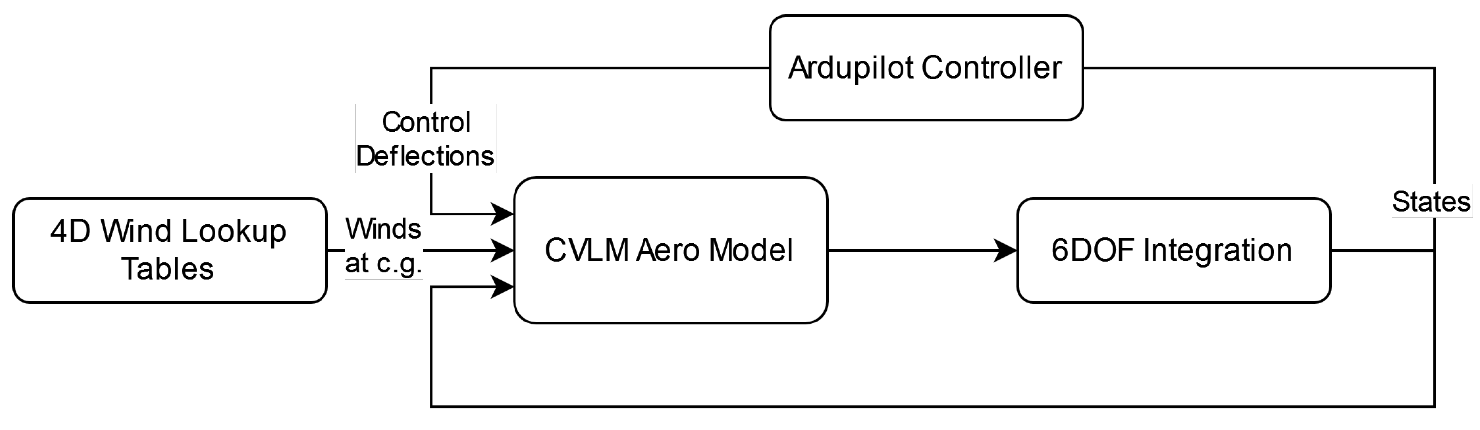
The primary objective of this paper is to develop a simulation environment capable of evaluating drone responses to arbitrary urban wind field models, as shown in Figure 1. This environment integrates aerodynamic modeling, flight dynamics, and atmospheric modeling to capture drone interactions with urban wind conditions. A Compact Vortex Lattice Method (CVLM) was employed to efficiently compute aerodynamic forces and moments. The aerodynamic model was implemented in MATLAB R2024b and integrated with a Simulink-based simulation framework that incorporates wind data interpolation, six-degree-of-freedom (6DOF) dynamics, and autopilot implementation via ArduPilot. High-fidelity wind fields were generated using Large Eddy Simulation (LES) within OpenFOAM, providing a temporally and spatially varying atmospheric environment. The simulation framework was further enhanced by Unreal Engine 5 visualizations, enabling a comprehensive analysis of drone behavior in urban turbulence conditions. This section details the implementation of these components and their role in creating the simulation environment.

2.1. Compact Vortex Lattice Aerodynamic Model

The aerodynamic forces and moments were calculated using a compact formulation of the classical vortex lattice method (CVLM), as outlined by Bunge [19,20]. This approach is suitable for low-speed, low-to-moderate angle-of-attack modeling and enables the rapid simulation of various configurations. CVLM captures the dominant inviscid nonlinear effects, cross-coupling, and configuration-specific aerodynamic factors like aspect ratio’s influence on lift curve slope and induced drag. These advantages make CVLM ideal for generating the large datasets required to analyze the dynamic responses of a drone in spatially and temporally varying urban wind fields.

The classical vortex lattice method solves the Laplace equation (Equation (1)) derived from the linearized Navier–Stokes equations using a superposition of simplified potential flow sources, most commonly horseshoe vortices or vortex ring components:

$${\nabla }^2\varphi =0$$

(1)

Based on the geometry of a drone’s planform, potential flow elementary flows, represented as vortex rings, are superimposed along mean camber lines, as represented by sets of vortices, and the circulation strength vector ($\Gamma$) is calculated using the non-penetrative boundary condition (Equation (2)):

$$\mathcal{A}\Gamma =-v_i$$

(2)

Here, $\mathcal{A}$ is the aerodynamic influence coefficient matrix and $v_i$ is the normal velocity at control points, derived from freestream conditions, drone motion, and turbulent gusts. Once $\Gamma$ is found, aerodynamic forces and moments are computed.

For moderate vortex counts, recalculating $\Gamma$ at each time step impacts the simulation run time. CVLM mitigates this by precomputing matrices $P_i$ and $Q_i$, which are unique to the aerodynamic lattice discretization. Forces and moments are then efficiently calculated using the following equations:

$$F_i=\rho X^T{P}_{i}X$$

(3)

$$M_i=\rho X^T{Q}_{i}X$$

(4)

$$X=\left[\begin{array}{c}V\\ \Omega \end{array}\right]$$

(5)

In these equations, $F_i$ and $M_i$ refer to the ith force or moment component, $\rho$ is air density, and X is the vector containing the three body-axis translational velocity components (V) and the three body-axis angular velocity components ($\Omega$). By avoiding the recalculation of $\Gamma$ and directly computing forces and moments, CVLM significantly reduces computation time at each simulation frame. Bunge and Kroo creatively incorporated control surface deflection effects by adjusting the normal vectors at the control points associated with the control surfaces. A slightly modified X vector, which includes control surface deflection angles, retains the computational efficiency of the aerodynamic force and moment calculations, as reflected in Equations (3) and (4), and is described in Ref. [19]. The CVLM aerodynamic force calculation methodology was implemented in our simulation framework using Quadair [20]. Readers seeking further details on the formulation of CVLM and the construction of the $P_i$ and $Q_i$ matrices are referred to Ref. [19].

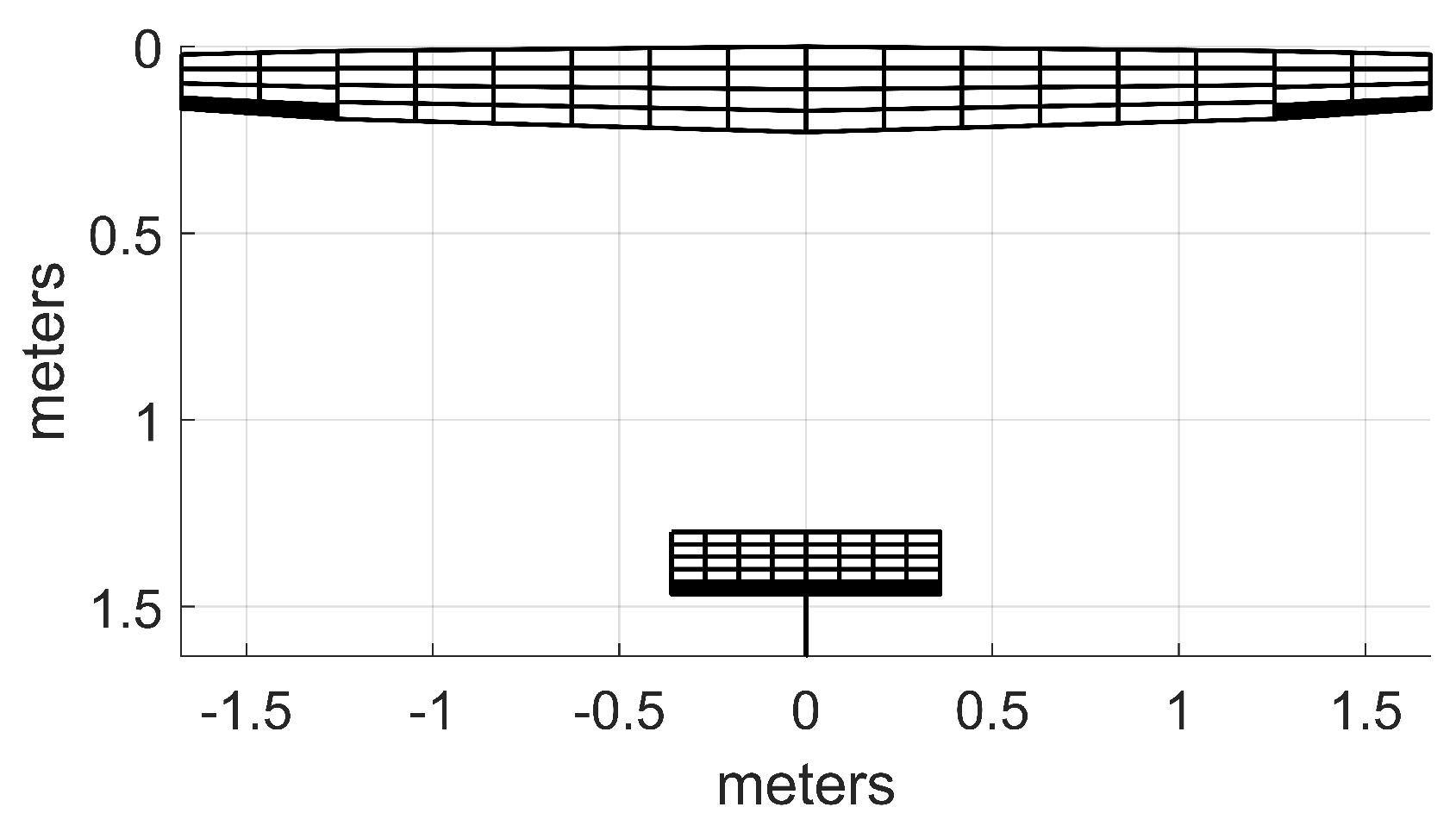
The aerodynamic grid of the planform used to generate the results of this paper is shown in Figure 2, with inertia properties and other considerations listed in

Table 1. Properties of the delivery drone vehicle.

Property	Value
Wing Airfoil	NACA 2412
Wing Taper Ratio	0.80
Vertical Tail Airfoil	NACA 0012
H-Stab. Taper Ratio	0.50
Dihedral Angle	$2^{\circ }$
Initial Airspeed	28 m/s
Wing Mass	7.984 kg
Fuselage Mass	5.988 kg
Stabilizer Mass	1.996 kg
Misc. Mass	3.992 kg
Total Mass	19.96 kg
Center of Gravity (CG)	(0.057, 0.0, 0.0) m
$I_{xx}$	20.91 kgm2
$I_{yy}$	29.57 kgm2
$I_{zz}$	45.64 kgm2
Wing Loading	29.0 kg/m2

. This configuration is based on the Zipline delivery drone [21] and was created based on photographs and publicly available information, including estimates of airspeed and total mass. The v-tail ruddervator featured on the original drone was projected into the body frame to simplify the control surface allocation logic. With the aerodynamic grid and inertia properties defined, Quadair was utilized in conjunction with an integration scheme in Simulink to simulate the response of the configuration through the urban wind field.

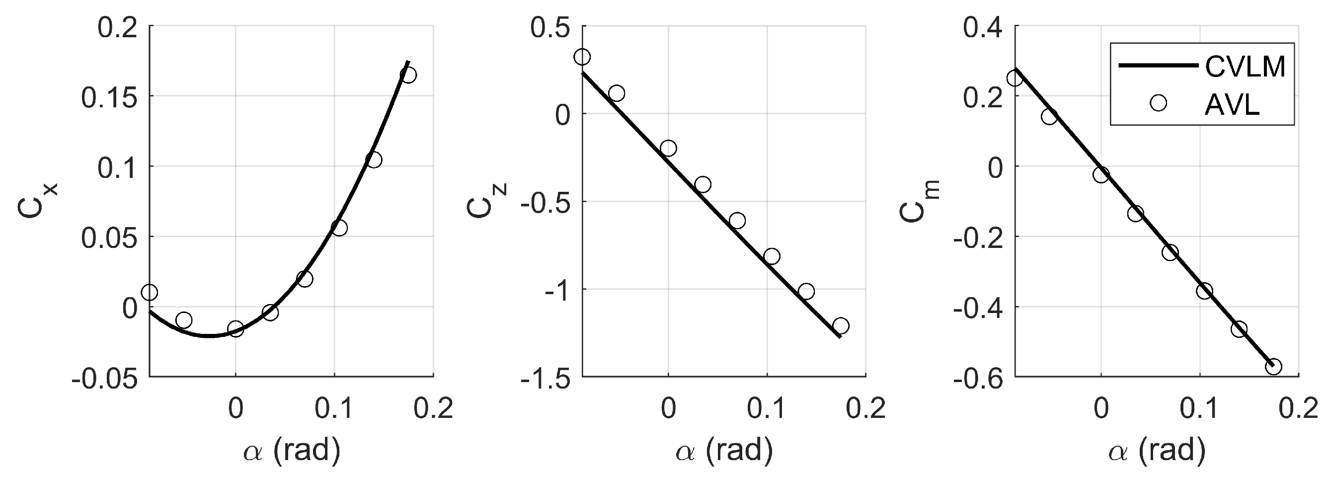
A comparison of the aerodynamic outputs between Quadair and AVL [22], a widely recognized vortex lattice method code, is presented in Figure 3 to validate the implementation of the Quadair codebase. Linear stability and control derivatives were extracted, and the short-period and phugoid dynamic modes were identified. The characteristics of these modes are summarized in

Table 2. Dynamic Mode Properties: Phugoid and Short Period.

Mode	Pole	Damping Ratio	Frequency (Hz)
Short Period	$-2.02\pm 2.38$i	$6.48\times {10}^{-1}$	$0.496$
Phugoid	$2.50\pm 4.49$i	$-5.56\times {10}^{-2}$	$0.072$

. Notably, the frequency of the fastest mode, the short period, is 0.5 Hz, supporting the choice of a 1-s sampling rate for the wind field implemented in the simulation environment.

2.2. Simulink Simulation Environment

Figure 4 summarizes the Simulink environment used to navigate the delivery drone through the wind fields. This simulation environment was created and executed on a modest consumer-grade desktop. The specifications of this desktop are listed in

Table 3. Hardware specifications of the computer used to generate the simulation results.

Component Specifications
CPU: AMD Ryzen 9 5900 × 12-cores
GPU: AMD Radeon RX 7600
RAM: 32 GB DDR4

.

Wind data were integrated into the simulation environment using built-in n-D Lookup Table blocks, with each block corresponding to one of the primary wind velocity components. The wind data were loaded into MATLAB as four-dimensional arrays, which were then passed to the n-D Lookup Tables. The dimensions of these arrays represent time, the North position, the East position, and altitude, enabling both spatial and temporal interpolation of the wind field. Each wind field domain occupied approximately 29 GB of storage when discretized onto a 3D rectilinear grid with 1 m spacing along all axes. The total size of the 4D arrays for each domain is 151 × 350 × 300 × 120. Before running the simulation, these values are compiled and allocated into RAM by Simulink. For the results presented in this paper, 30 m altitude chunks were loaded into the n-D Lookup Tables, keeping RAM usage well below the system’s capacity. Larger domain sizes can be accommodated by this simulation environment, particularly if RAM capacity is increased—modern consumer desktops support up to 192 GB.

At each time step, the wind vector is combined with the drone’s body velocities to form the state information matrix, as shown in Equation (5), incorporating the wind effects into the CVLM force and moment calculations. This combination of the wind vectors is described by Equations (6) and (7), consistent with Ref. [23] and captures the instantaneous change in the aerodynamic angles. This is achieved by projecting the wind magnitudes described in the inertial axis onto the drone body frame using the rotation matrix (${\mathcal{R}}_v^b$). The wind velocities described in the body axis ($V_w^b$) are then subtracted from the drone body velocities to define the velocities of the drone relative to the air ($V_b$), which are used for the calculation of the aerodynamic forces and moments.

$${\mathbf{V}}_w^b=\left(\begin{array}{c}{u}_w\\ v_w\\ w_w\end{array}\right)={\mathcal{R}}_v^b(\varphi ,\theta ,\psi )\left(\begin{array}{c}{w}_n\\ w_e\\ w_d\end{array}\right).$$

(6)

$$V_b=\left(\begin{array}{c}u-u_w\\ v-v_w\\ w-w_w\end{array}\right)$$

(7)

The Euler attitude representation of the 6DOF block native to the Aerospace Blockset is then used to integrate the equations of motion forward to find the updated states of the vehicle. Simulink handles the selection of the integration scheme and time step automatically. The states are then sent to ArduPilot using Transmission Control Protocol (TCP) network communication [24], and control input pulse-width modulation (PWM) signals are received. These signals are converted to commanded deflections, and actuator dynamics are applied. The actuator dynamics are represented using the transfer functions provided in

Table 4. Actuator dynamic transfer functions.

Elevator	Aileron	Rudder
${\displaystyle \frac{{\delta }_e}{{\delta }_{ec}}}={\displaystyle \frac{8}{s+10}}{e}^{-0.065s}$	${\displaystyle \frac{{\delta }_a}{{\delta }_{ac}}}={\displaystyle \frac{40}{s+12}}{e}^{-0.060s}$	${\displaystyle \frac{{\delta }_r}{{\delta }_{rc}}}={\displaystyle \frac{10}{s+10}}{e}^{-0.065s}$

, provided by Schulze et al. [25] for a representative small UAS platform.

ArduPilot version 4.5 [26], an open-source autopilot software suite that is widely used in the drone community, was integrated with Simulink to enable waypoint tracking and navigation. This integration was achieved by running the autopilot software concurrently with Simulink and exchanging data over TCP. The states of the drone (attitude, position, velocity, etc.) are sent from Simulink to ArduPilot, which in turn sends control deflection inputs back to Simulink. The network communication protocol is implemented using Simulink blocks available on the GitHub repository repository hosting the ArduPilot codebase [27].

The ArduPlane control architecture consists of nested PID control loops. The Total Energy Control System (TECS) runs concurrently and manages airspeed and altitude by adjusting throttle and pitch. Due to the TCP’s communication with the software, sensor fusion is turned off and the outputs from the simulation environment are accepted as the states.

The tuning of the control law gains was handled using the Autotune mode in ArduPilot. During simulation, the drone was flown using a control stick, and the software automatically adjusted the gains based on the drone’s response to pitch, roll, and yaw commands. All parameters in ArduPilot were reset to their default values before tuning, including the AUTOTUNE_LEVEL parameter, which dictates the aggressiveness of the tuning. The default value of AUTOTUNE_LEVEL is 6, corresponding to a medium level of tuning. The gains obtained from the autotune and used to generate the results of this paper are outlined in Appendix A.

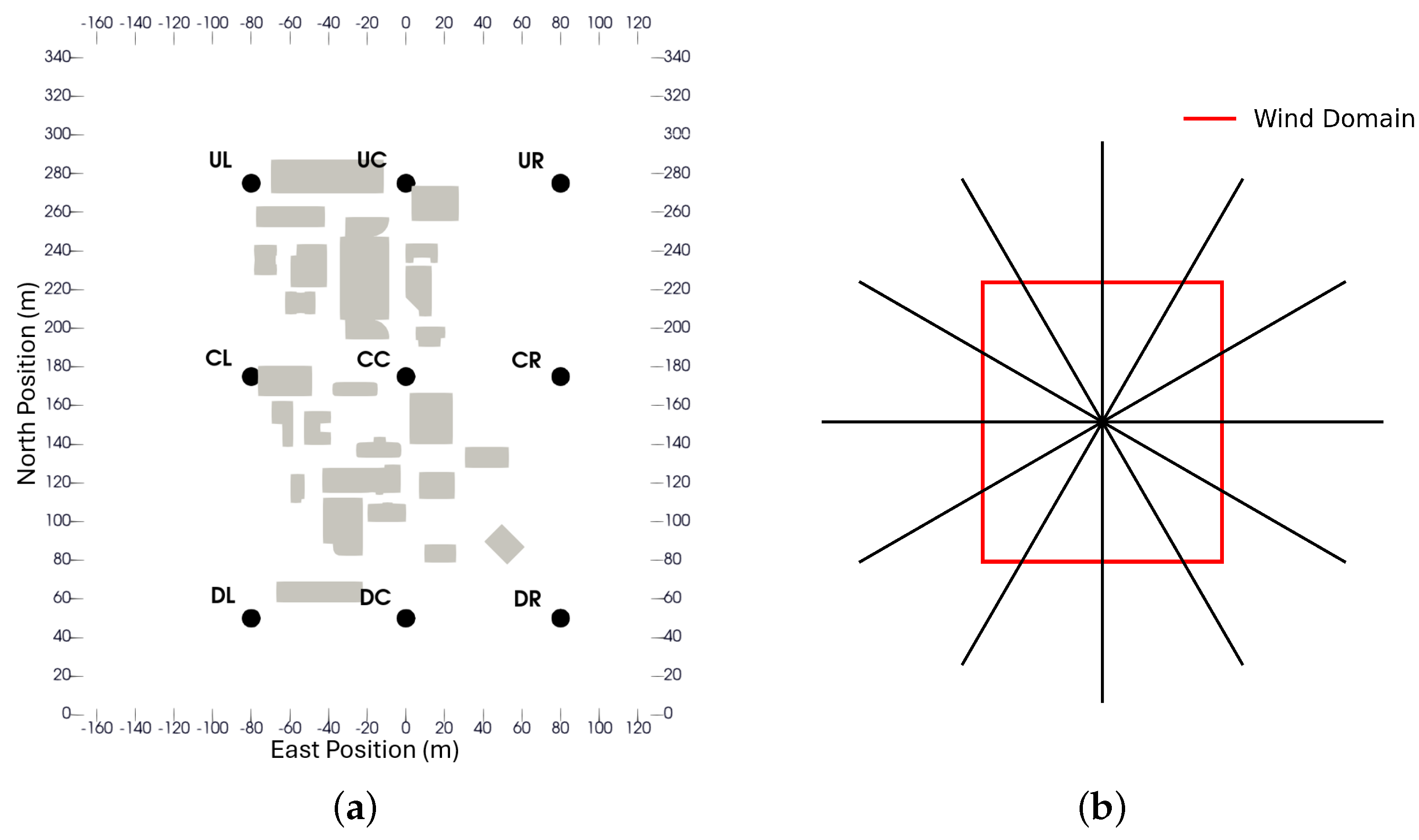
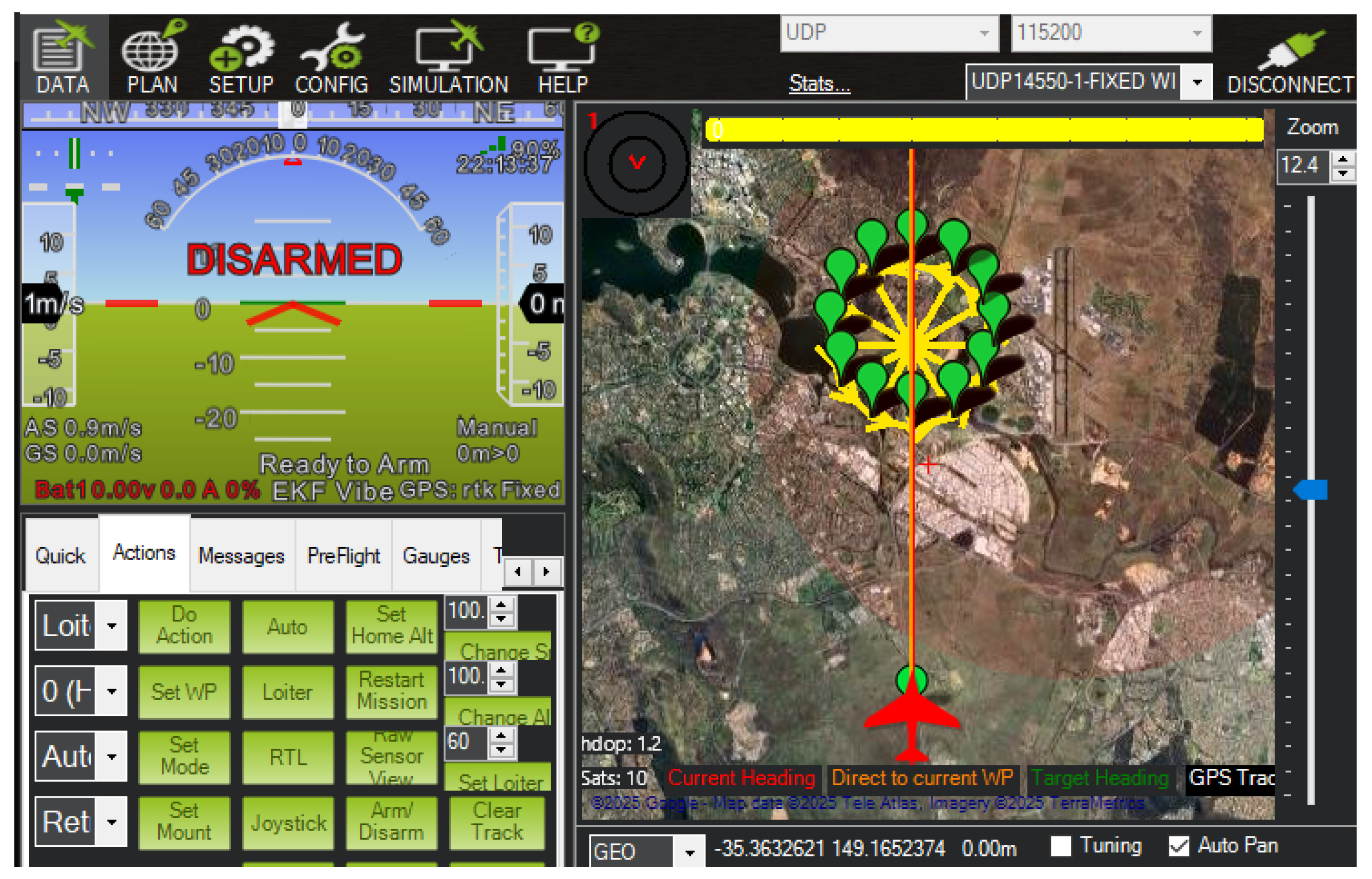
ArduPilot executed the mission profiles depicted in Figure 5. To capture distinct wind structures and spatial variations in the environment, these azimuths were flown around nine central locations (Figure 5a). Center points, labeled with identifiers such as UL, UC, and UR, define a grid over the cityscape to enhance the spatial diversity of the airspace sampled for vehicle impact analysis. Azimuths were varied in increments of ${30}^{\circ }$ (Figure 5b) to ensure the configuration interacted with the wind field from different orientations as each center point was approached. The Mission Planner interface, shown in Figure 6, was then used to begin the test plan and collect the results.

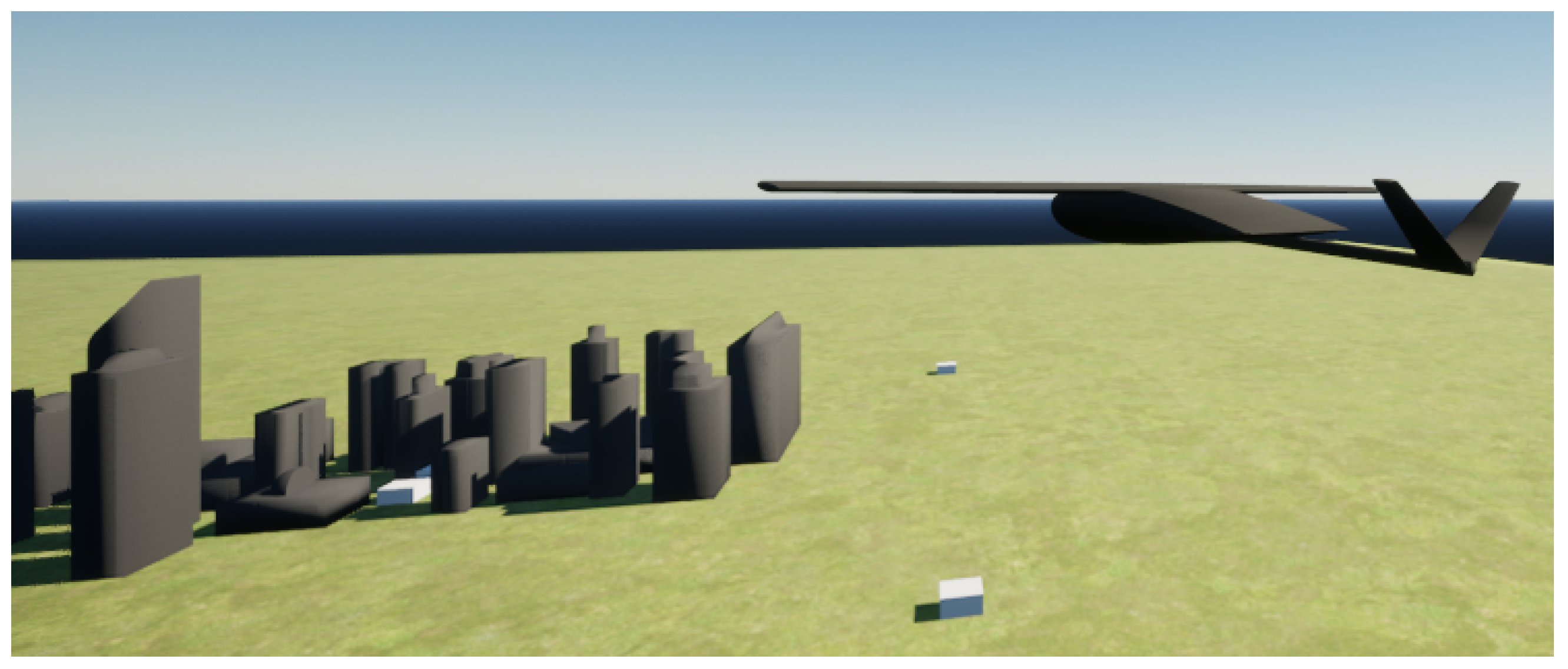
The simulation environment supports the ability to visualize the simulation using Unreal Engine 5 (UE5). This ability is optional and can be ignored if all computational resources are necessary to run the simulation. Custom environments and drones can easily be created using UE5 and Computer-Aided Design (CAD) tools. Figure 7 demonstrates these capabilities, where the city used to create the LES wind fields and a representation of a delivery drone are integrated into the simulation environment.

2.3. Atmospheric Modeling

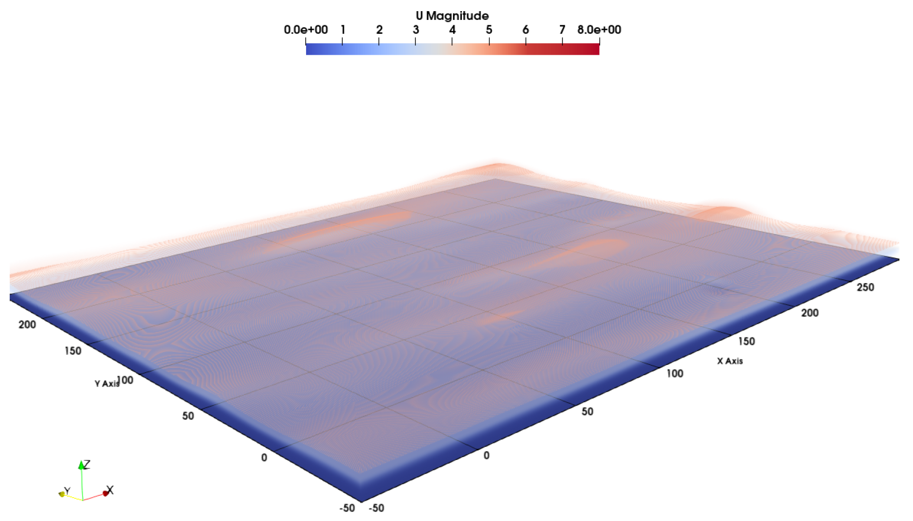
A realistic atmospheric wind field was generated using computational fluid dynamics (CFD) solver Open-source Field Operation and Manipulation (OpenFOAM) [28]. OpenFOAM could be characterized as a numerical solver toolbox used to perform CFD simulations for various fluid flow problems like turbulence modeling, combustion, and multi-phase flow problems [29]. Large-Eddy Simulation (LES) methodology for turbulence modeling was used to generate an atmospheric boundary layer with turbulent wind flow to interact with a typical urban landscape with buildings.

2.3.1. Governing Equations

In this study, we simulated the wind field by solving the incompressible Navier–Stokes equations, using the Boussinesq approximation to account for buoyancy effects in a Cartesian coordinate system. We employed a Large-Eddy Simulation (LES) framework coupled with a Subgrid-Scale (SGS) turbulence model to capture turbulent scales that remain unresolved. Detailed descriptions of the continuity and momentum equations, numerical methods, and the SGS model are provided briefly here. For further details, readers may refer to our previous work [15].

$${\displaystyle \frac{\partial u_i}{\partial x_i}}=0$$

(8)

$${\displaystyle \frac{\partial u_i}{\partial t}}+{\displaystyle \frac{\partial u_i{u}_j}{\partial x_j}}=-{\displaystyle \frac{1}{\rho }}{\displaystyle \frac{\partial p}{\partial x_i}}+\nu {\displaystyle \frac{{\partial }^2{u}_i}{\partial x_j\partial x_j}}$$

(9)

Filtering the above equations, and after simplification, we obtained the following:

$${\displaystyle \frac{\partial \overline{u_j}}{\partial x_j}}=0$$

(10)

$${\displaystyle \frac{\partial \overline{u_i}}{\partial t}}+{\displaystyle \frac{\partial \overline{u_i{u}_j}}{\partial x_j}}=-{\displaystyle \frac{1}{\rho }}{\displaystyle \frac{\partial \overline{p}}{\partial x_i}}+\nu {\displaystyle \frac{{\partial }^2\overline{u_i}}{\partial x_j\partial x_j}}$$

(11)

It is impossible to determine the quantity ${\displaystyle \frac{\partial \overline{u_i{u}_j}}{\partial x_j}}$, but the quantity ${\displaystyle \frac{\partial {\overline{u}}_i{\overline{u}}_j}{\partial x_j}}$ is known. Substituting ${\tau }_{ij}={\displaystyle \frac{\partial \overline{u_i{u}_j}}{\partial x_j}}-{\displaystyle \frac{\partial {\overline{u}}_i{\overline{u}}_j}{\partial x_j}}$ yields

$${\displaystyle \frac{\partial \overline{u_i}}{\partial t}}+\overline{u_j}{\displaystyle \frac{\partial \overline{u_i}}{\partial x_j}}=-{\displaystyle \frac{1}{\rho }}{\displaystyle \frac{\partial \overline{p}}{\partial x_i}}+\nu {\displaystyle \frac{{\partial }^2\overline{u_i}}{\partial x_j\partial x_j}}-{\displaystyle \frac{\partial {\tau }_{ij}}{\partial x_j}}$$

(12)

where $u_i$ (with $i=1,2,3$) denotes the velocity components, and ${\tau }_{ij}$ represents the sub-grid scale stress tensor.

When combined with the Boussinesq hypothesis, the sub-grid stress can be written as follows:

$${\tau }_{ij}=-2{\nu }_t{\overline{S}}_{ij}+{\displaystyle \frac{1}{3}}{\tau }_{kk}{\delta }_{ij}$$

(13)

where,

• ${\nu }_t={\displaystyle \frac{{\mu }_t}{\rho }}$, ${\mu }_t$ is the turbulent viscosity.
• ${\overline{S}}_{ij}={\displaystyle \frac{1}{2}}\left({\displaystyle \frac{\partial {\overline{u}}_i}{\partial x_j}}+{\displaystyle \frac{\partial {\overline{u}}_j}{\partial x_i}}\right)$

For LES Sub-Grid-Scale (SGS) closure, the Wall-Adaptive Local Eddy viscosity (WALE) model [30] was used. The effects of turbulent wall surface and momentum transfer were considered, setting it apart from the traditional Smagorinsky model of turbulence closure. The turbulent viscosity was computed using the following:

$${\nu }_t={\left(C_w\Delta \right)}^2{\displaystyle \frac{{\left({\overline{S}}_{ij}^d{\overline{S}}_{ij}^d\right)}^{\frac{3}{2}}}{{\left({\overline{S}}_{ij}{\overline{S}}_{ij}\right)}^{\frac{5}{2}}+{\left({\overline{S}}_{ij}^d{\overline{S}}_{ij}^d\right)}^{\frac{5}{4}}}}$$

(14)

where $\Delta$ is the filter scale determined by the lengths of the element in x,y,z directions, $C_w=0.325$, and ${\overline{S}}_{ij}^d$ is computed using

$${\overline{S}}_{ij}^d={\displaystyle \frac{1}{2}}\left({\overline{g}}_{ij}^2+{\overline{g}}_{ji}^2\right)-{\displaystyle \frac{1}{3}}{\delta }_{ij}{\overline{g}}_{kk}^2$$

(15)

Here,

$${\overline{g}}_{ij}={\displaystyle \frac{\partial \overline{u_i}}{\partial x_j}}$$

(16)

2.3.2. Simulation Setup and Domain

To generate a dynamically evolving turbulent inflow for the LES simulation, we specify not only the inlet velocity field but also the associated Reynolds stress components and eddy length scales. These turbulent inflow conditions were obtained from a precursor Reynolds-Averaged Navier–Stokes (RANS) simulation, as recommended in [15,31]. In this setup, the RANS domain’s outlet dimensions are matched to the LES inlet to ensure consistency between the simulations. A streamwise domain length of 5 km was chosen, and the inlet wind profile was defined using a logarithmic law with a reference height ($z_{ref}$), at which the wind speed was set to 8 m/s, following [15,31]. The LES inlet boundary condition was implemented using OpenFOAM’s atmBoundaryLayer method, with a ground-plane surface roughness length ($z_0$) of 0.33 m [32].

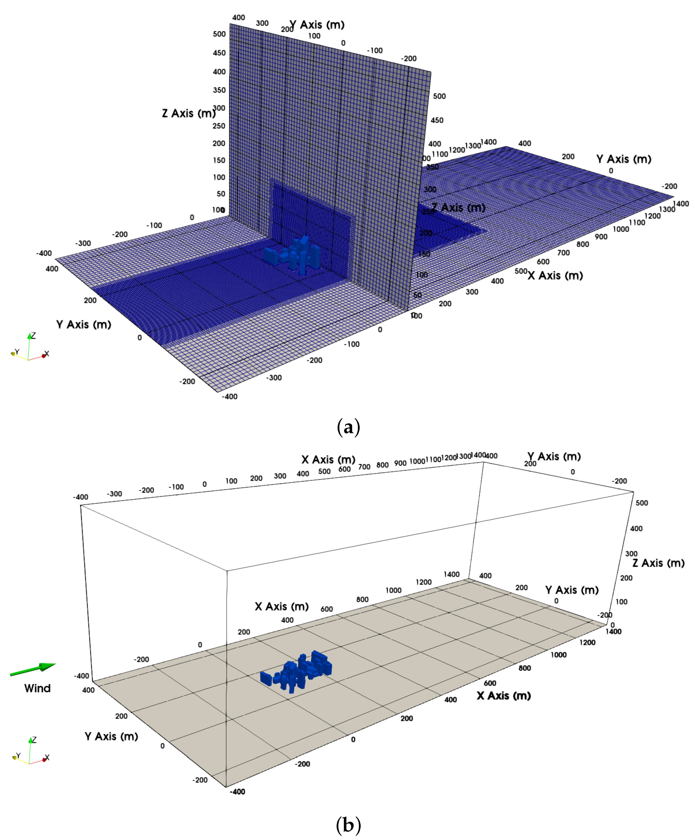
The LES simulation domain, shown in Figure 8, was selected based on the recommendations of Frank et al. [33] to ensure that the blockage ratio remained below 3%. The blockage ratio was calculated by assuming that the buildings, which occupy the entire designated area, form a continuous obstruction. The domain dimensions were defined relative to the height of the tallest building ($H=80\mathrm{m}$): the domain was $6.75H$ high, $8.75H$ wide, and $23H$ long, with an upstream extension of approximately $4H$ and a downstream extension of about $15H$.

3. Results

3.1. Flow-Field Characterization

The three-dimensional isometric views of the resulting wind fields obtained from snapshots of the LES simulations are presented in Figure 9 for the various inflow conditions relative to the cityscape. For comparison, an isometric view of the domain without the presence of the buildings is shown in Figure 10, which exclusively features the influence of the precursor simulation. The presence of the buildings creates turbulent structures that extend several meters above the buildings, much higher than the structures seen in Figure 10.

To assess the city’s impact on the overall wind field conditions at various altitudes, the averaged Turbulent Kinetic Energy (TKE), denoted as k, was employed. This metric was calculated using Reynolds decomposition, as outlined in Equations (17)–(19), providing a value at each grid point that characterizes the intensity of the velocity fluctuations.

$${\overline{{\mathbf{U}}^{\prime }}}^2={\displaystyle \frac{1}{N}}\sum _{i=0}^N{\left({\mathbf{U}}_i-\overline{\mathbf{U}}\right)}^2$$

(17)

where $\overline{\mathbf{U}}$ is the mean velocity vector,

$$\overline{\mathbf{U}}={\displaystyle \frac{1}{N}}\sum _{i=0}^N\left({\mathbf{U}}_i\right)$$

(18)

where $\mathbf{U}$ is the velocity vector with components $u,v,w$

$$k={\displaystyle \frac{1}{2}}\left(\overline{u^{\prime 2}}+\overline{v^{\prime 2}}+\overline{w^{\prime 2}}\right)$$

(19)

where k is the average turbulent kinetic energy.

Figure 11 shows TKE values at various altitudes for the nine central points under the $0^{\circ }$ inflow condition, which are depicted in Figure 5a as reference locations for different mission profiles. Based on the results, altitudes of 60 m and 100 m were selected to represent heavy and light turbulence cases, respectively, with 60 m being in close proximity to the tops of most buildings. To assess the impact of the buildings on TKE, the figure also includes TKE values at the same exact locations with the influence of the buildings removed, as shown in Figure 10.

3.2. Flight Dynamics Results

The configuration was flown through the wind fields using the mission profile defined in Figure 5 at initial altitudes of 60 m and 100 m. Temporal interpolation was performed as the drone enters the grid, with the time being reset upon exiting. Simulations were conducted at start times of 0 s, 20 s, 40 s, 60 s, 80 s, 100 s, 120 s, and 125 s. A step size of 20 s was chosen as it represents half the time required for a wind structure originating at the furthest building upwind to fully exit the grid, ensuring sufficient temporal resolution to capture interactions with the turbulence. Figure 12 illustrates all paths through the $0^{\circ }$ and ${180}^{\circ }$ wind fields, highlighting the extent of the grid exploration and the number of azimuths covered. This dense study of the grid was enabled through the efficiency of the aerodynamic solver, which allows the simulation to run as roughly 2× to 3× real time.

The flight dynamics plots for the cases that resulted in the maximum g-loads at each altitude are shown in Figure 13 and Figure 14. At an altitude of 100 m, the wind structures were highly localized (Figure 13b), leading to the maximum g-load occurring when the drone encountered a singular region of high vertical wind velocity. In contrast, at 60 m (Figure 14b), the wind structures were more widespread, causing the maximum g-loading to occur along the path on which the wind field gradient was greatest, which occurred as the drone left the shadow of the tallest building and was bombarded with a large vertical velocity change.

Table 5. Max G-Loading Across Wind Fields and Models.

Category	Condition	G Loading 60 m	G Loading 100 m
LES Wind	0°	2.87	2.14
	90°	3.00	1.30
	135°	3.19	1.42
	180°	3.50	1.93
LES No City	-	1.57	1.27
von Kármán	2.28 m/s, median LES	1.16	1.14
	7.72 m/s, light	1.57	1.46
	15.43 m/s, medium	2.25	1.92

summarizes the results by presenting the maximum G-loadings for all cases at inflow conditions of $0^{\circ }$, ${90}^{\circ }$, ${135}^{\circ }$, and ${180}^{\circ }$. To isolate the effects of the city, the urban area was removed, and the LES field was regenerated to eliminate any influence from the buildings. A single inflow direction was analyzed, as the lack of unique spatial features made additional directions unnecessary and redundant. The same mission profile depicted in Figure 5 was used to ensure consistency. The maximum G-loading at each altitude, shown in Table 5, highlights the disparity in the loading of the drone when buildings are present compared to the scenario without them.

The configuration was also evaluated using a traditional turbulence model through the low-altitude von Kármán model, implemented via the built-in Simulink block [34]. At low altitudes, the only required inputs were the altitude and the wind magnitude at 6 m, commonly referred to as $W_{20}$ or $u_{20}$, denoting 20 feet in regulatory documents such as MIL-STD-1797. Three wind magnitudes were explored: 2.28 m/s, representing the median wind magnitude of the LES inflow condition at 6 m; 7.72 m/s (15 knots), categorized as light turbulence; and 15.43 m/s (30 knots), categorized as medium turbulence.

Projections of the maximum g-loading experienced across the entire grid are presented in Figure 15a,c. These plots correspond to the inflow conditions that produced the maximum g-loading at each altitude, as detailed in Table 5. The plots were generated using MATLAB’s griddata function, which interpolates the data to fill gaps in the grid where no direct encounters occurred. Notably, these figures closely align with the slice plots of the temporally averaged TKE metric at the corresponding altitudes, shown in Figure 15b,d. Comprehensive maximum g-loading projections and TKE plots for all inflow conditions and altitudes are included in the Appendix B.

4. Discussion

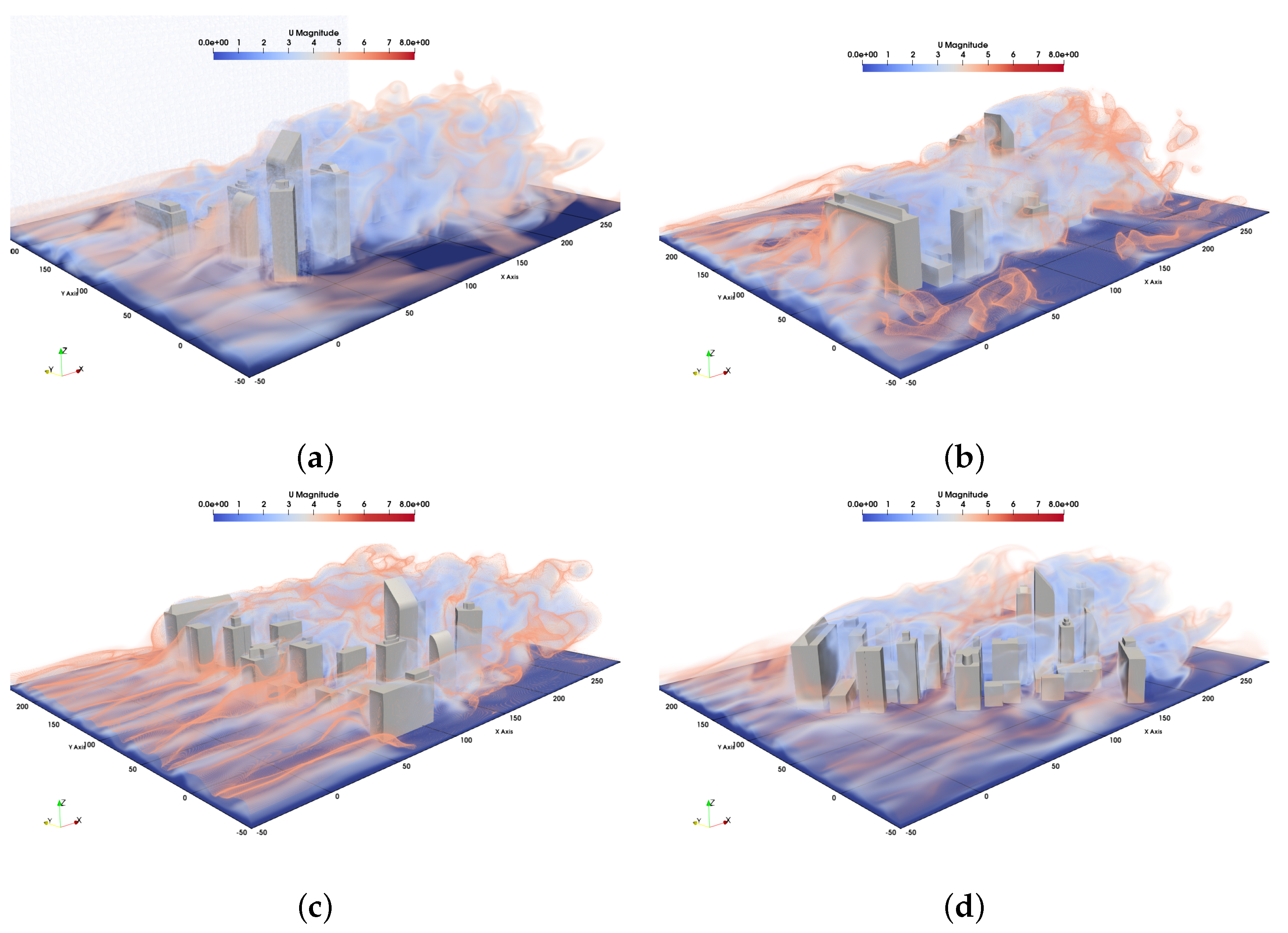
The results underscore the inadequacy of existing turbulence models in replicating urban environmental conditions. As highlighted in Table 5, the von Kármán turbulence model, with a magnitude of 15.43 m/s at 6 m altitude, severely underpredicts the maximum g-loading experienced in the LES wind at the 60 m target altitude. This discrepancy is concerning because the 15.43 m/s is typically categorized as medium-level turbulence, yet it fails to represent the LES wind conditions at 6 m altitude, which were found to be 2.28 m/s. This mismatch between traditional turbulence model categorizations and actual urban wind conditions can lead to an underestimation of g-loadings during the preliminary design phase, posing significant challenges for the certification process. These findings highlight an urgent need to develop new turbulence models specifically designed for certifying drones in urban environments.

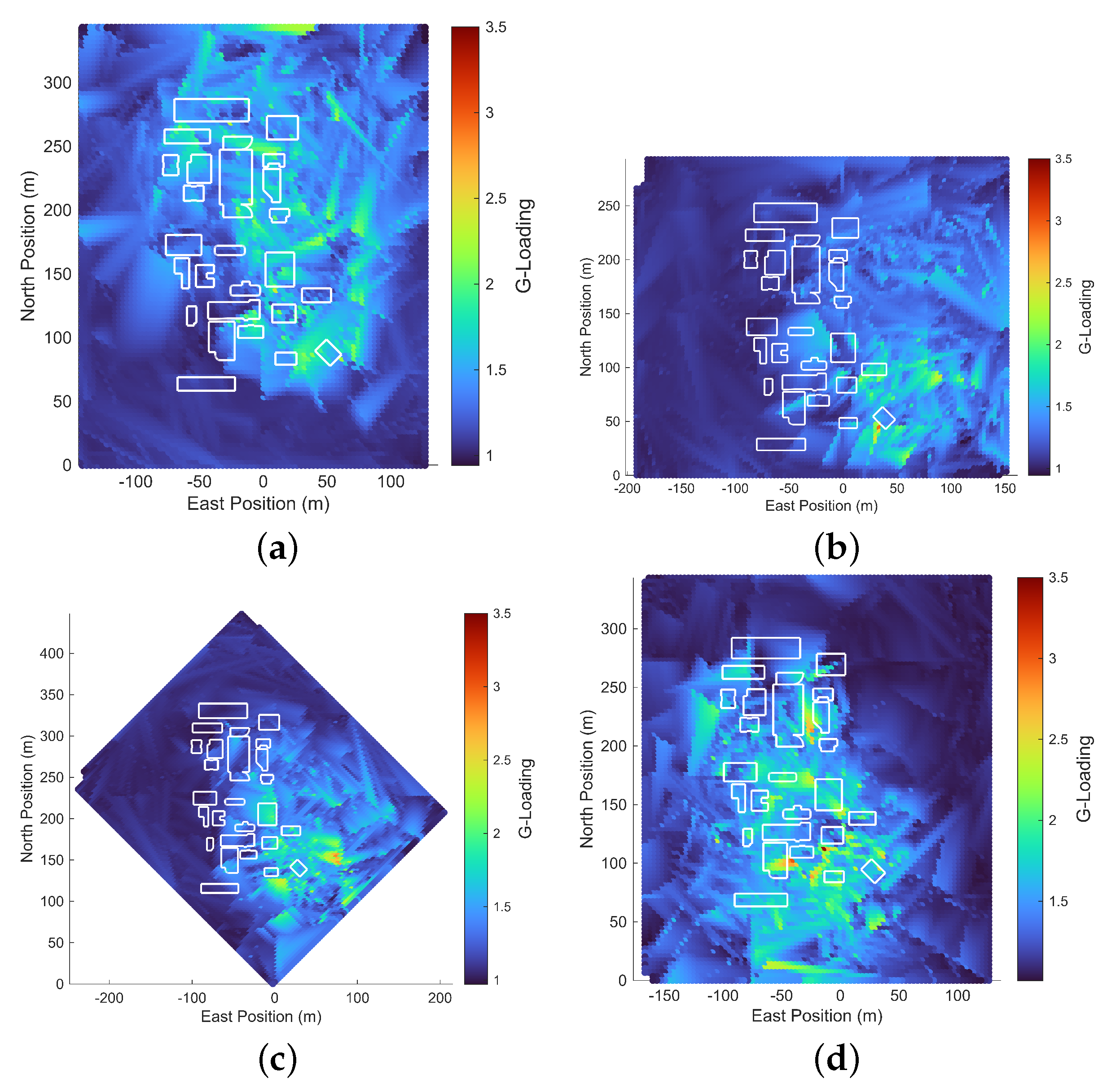
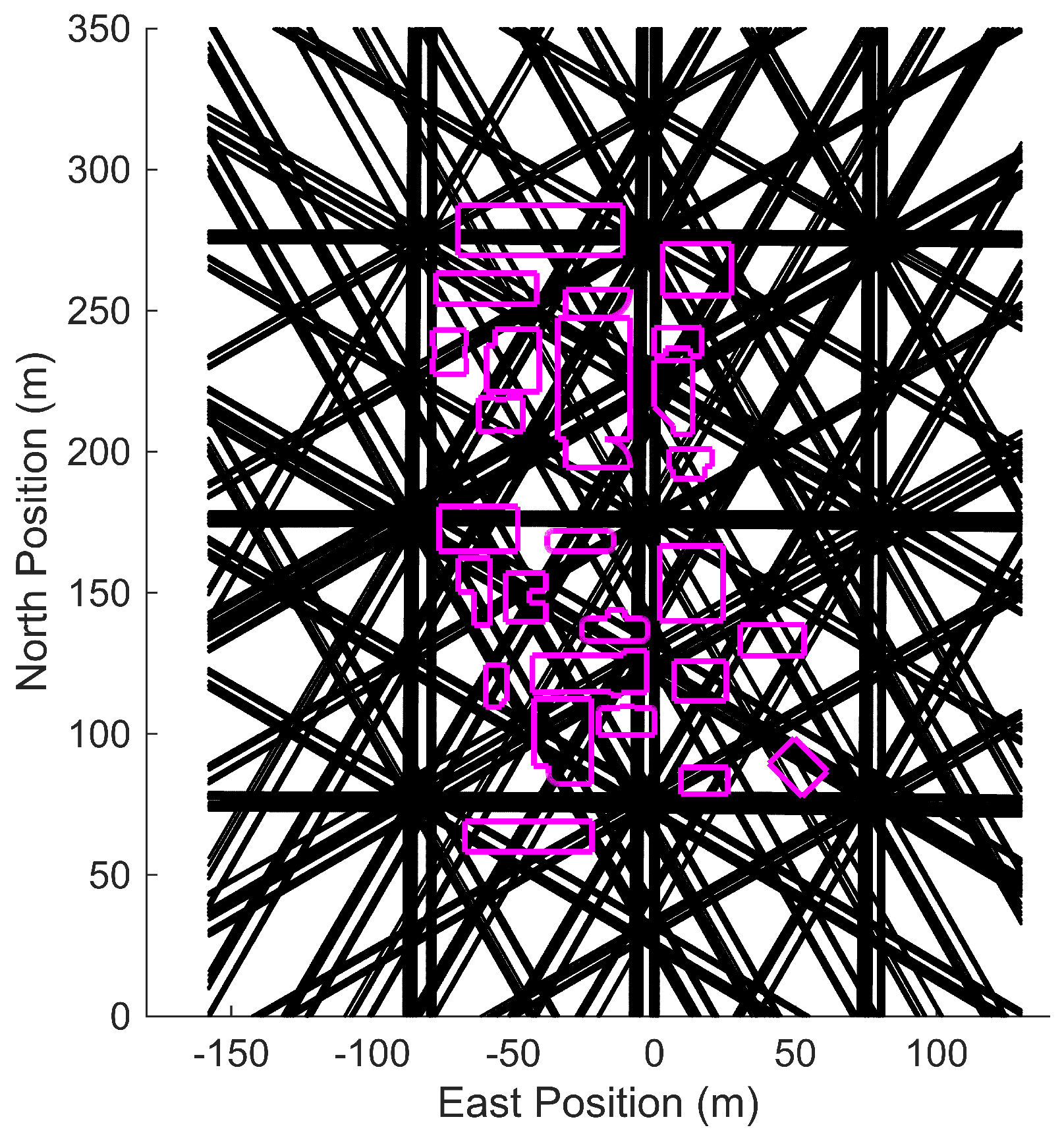
Traditional turbulence models lack spatial significance, which limits their applicability to urban environments. In contrast, the methodology described above allows drone responses to be modeled spatially, enabling the zoning of urban areas based on expected maximum g-loading, as illustrated in figures such as Figure 15a,c. This approach identifies challenging locations for drone navigation and categorizes them according to the inflow conditions. With a sufficiently large database, this information can be leveraged to optimize mission paths through urban environments, particularly for applications like package delivery.

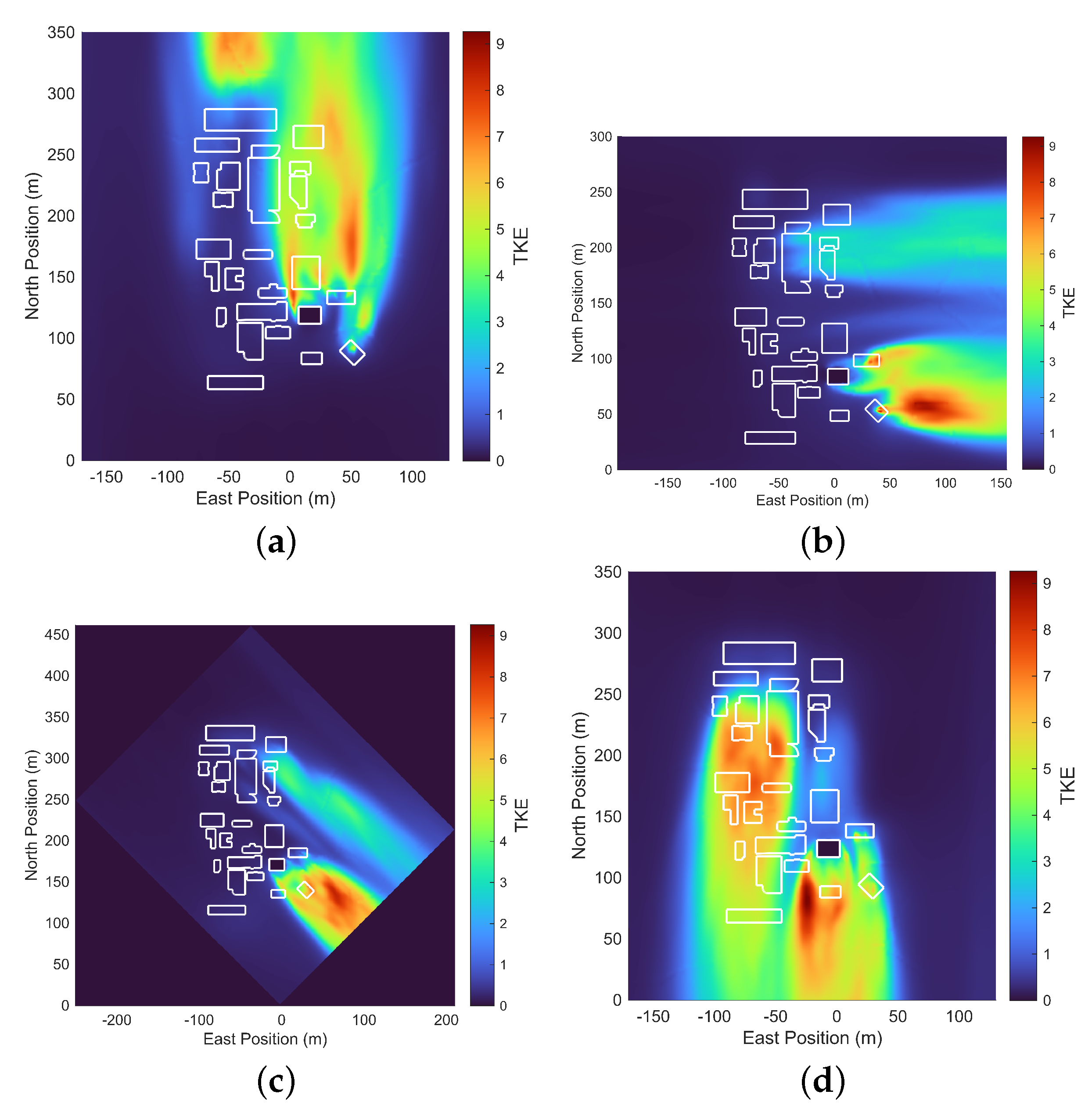
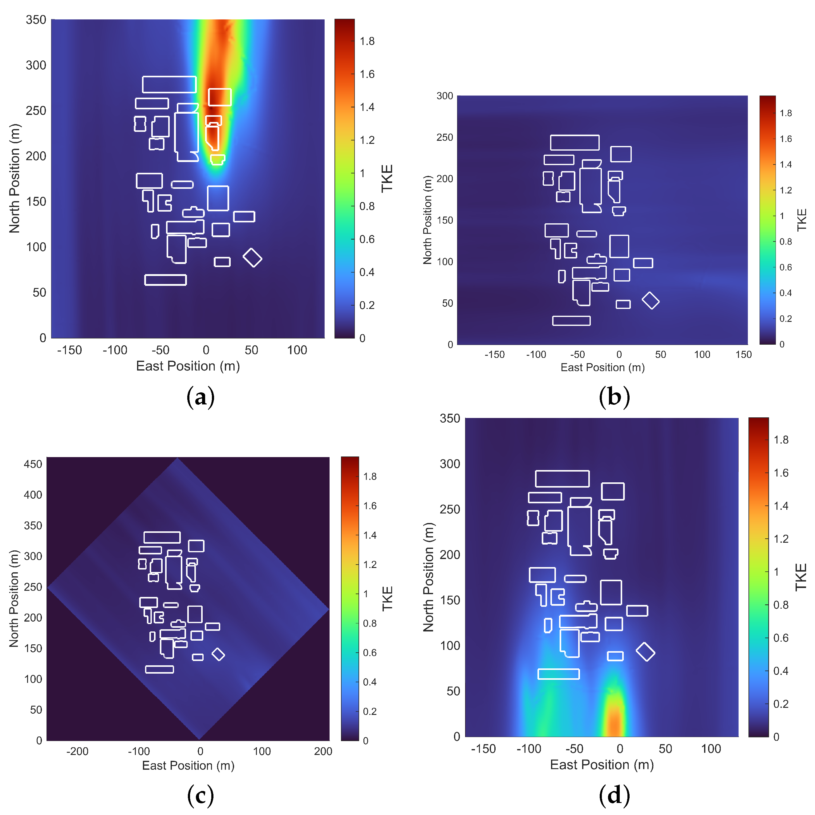
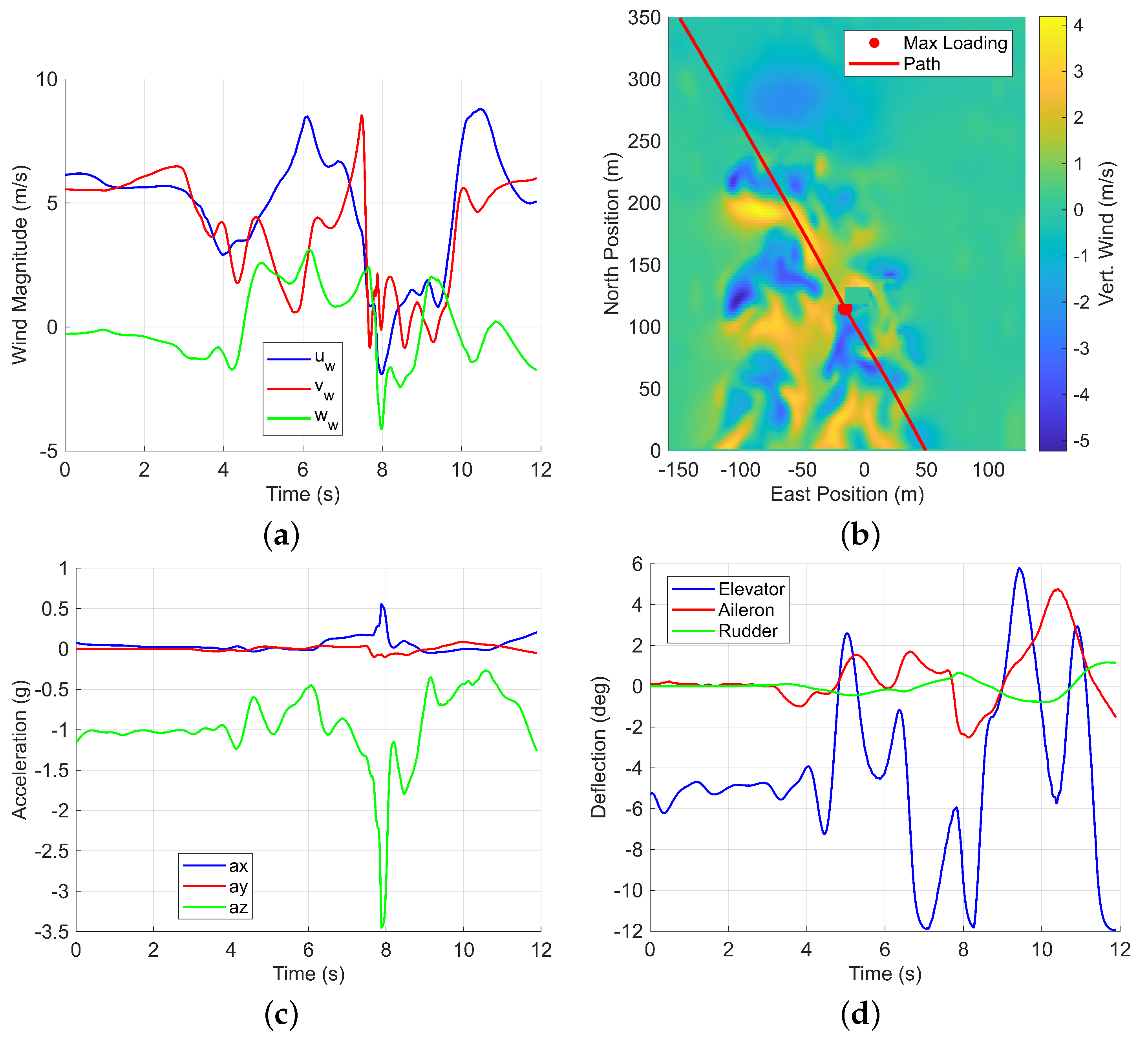
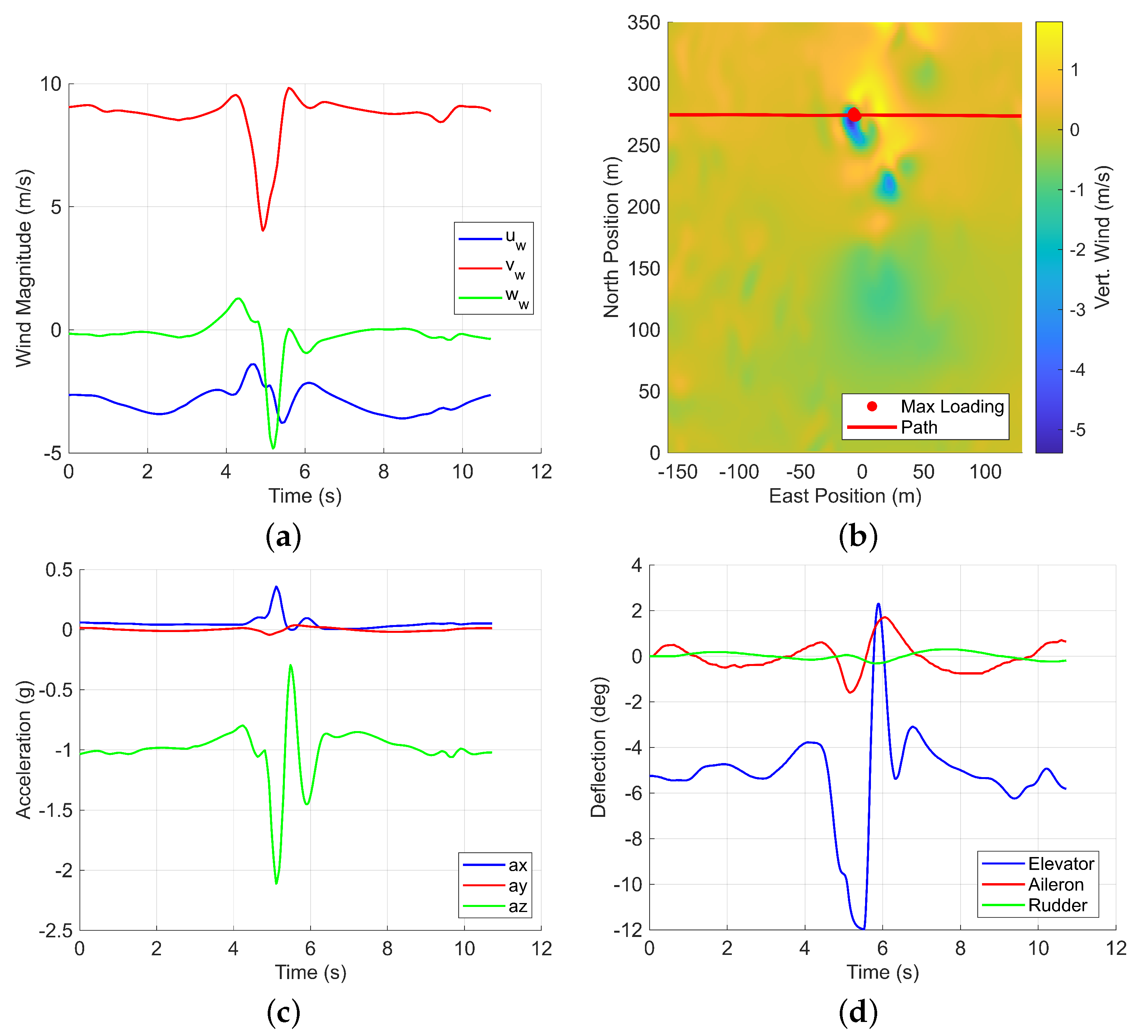
The TKE metric provides valuable insight into the locations of higher g-loads when compared to the maximum g-loading plots. As shown in Figure 15, maximum g-loadings consistently occur in areas with significant TKE gradients. For instance, these gradients are particularly evident when the drone emerges from the profile of the tallest building, as depicted in Figure 15a,b. This observation suggests that focusing on paths along these TKE gradients can streamline the identification of the, maximum expected g-loads and their corresponding zones, saving both time and effort. Future work will explore the significance of the TKE metric in this type of analysis in greater detail.

5. Future Research Directions

Future work will also focus on further validating both the drone and wind field models. While the CVLM model of the drone effectively represents longitudinal dynamics, it has notable shortcomings, including an underestimation of drag and an overprediction of the elevator and aileron control powers [35]. The validation process for aerodynamic models through flight testing is well established for fixed-wing aircraft via system identification methods [36], although the error bounds for the aerodynamic terms tend to be large for smaller drones, like the one used in this study [35].

A more complex challenge lies in validating the wind field derived from the LES. Although estimations of the severity of disturbances experienced by an aircraft were successfully demonstrated for both fixed-wing and rotorcraft platforms through the Eddy-Dissipation Rate (EDR) and other gust idealizations [2,10,37,38], these processes were never accompanied by estimations of the inflow conditions of the environment. Given the inherent difficulties of capturing inflow conditions during flight testing, an alternative approach may involve using subscale cityscape models in a wind tunnel environment, where inflow conditions can be precisely controlled. Ultimately, these challenges must be addressed to develop a validated urban wind field model capable of supporting disturbance rejection analysis efforts. The simulation framework is also expected to provide a useful tool for research on optimizing flight routes through urban areas from an efficiency and flight endurance perspective, as energy consumption will be an important performance parameter for urban drones.

6. Conclusions

A flexible simulation environment, combining vehicle open-loop dynamics models in Simulink and control loop closures via the common drone Ardupilot flight control software, was created to evaluate fixed-wing AAM platforms in challenging wind environments. Due to the lack of existing urban turbulence models, LES CFD simulations of a notional cityscape were generated following the best practices available in the research literature. The urban operational environment was thoroughly explored for constant wind magnitudes through varying wind inflow azimuth and simulating drone flight and wind interactions via a one-way coupling approach. Phenomena, such as the non-repeating wind patterns and temporal/spatial variation in the wind effects, encouraged the thorough sampling of the domain with several initial azimuths, start times, and centralized points, and the response of the drone was recorded for each encounter.

The work presented is novel as it expands upon prior research efforts outlined in the literature through integrating a CVLM aerodynamic solver capable of accommodating arbitrary fixed-wing platforms, rather than relying on preexisting models, which are limited to specific airframes. Unlike previous studies that constrained turbulent interactions to simplified two-dimensional, temporally frozen fields [16], or an RANS database [13], this simulation environment captures the full spatiotemporal variation in an LES-generated urban wind field. This allows for the rapid deployment and evaluation of a wide range of fixed-wing AAM configurations, enabling the efficient computation of their dynamic responses to the complex, time-varying wind environments commonly found in urban settings.