

The Synergistic Effects of GCPs and Camera Calibration Models on UAV-SfM Photogrammetry


Abstract
1. Introduction
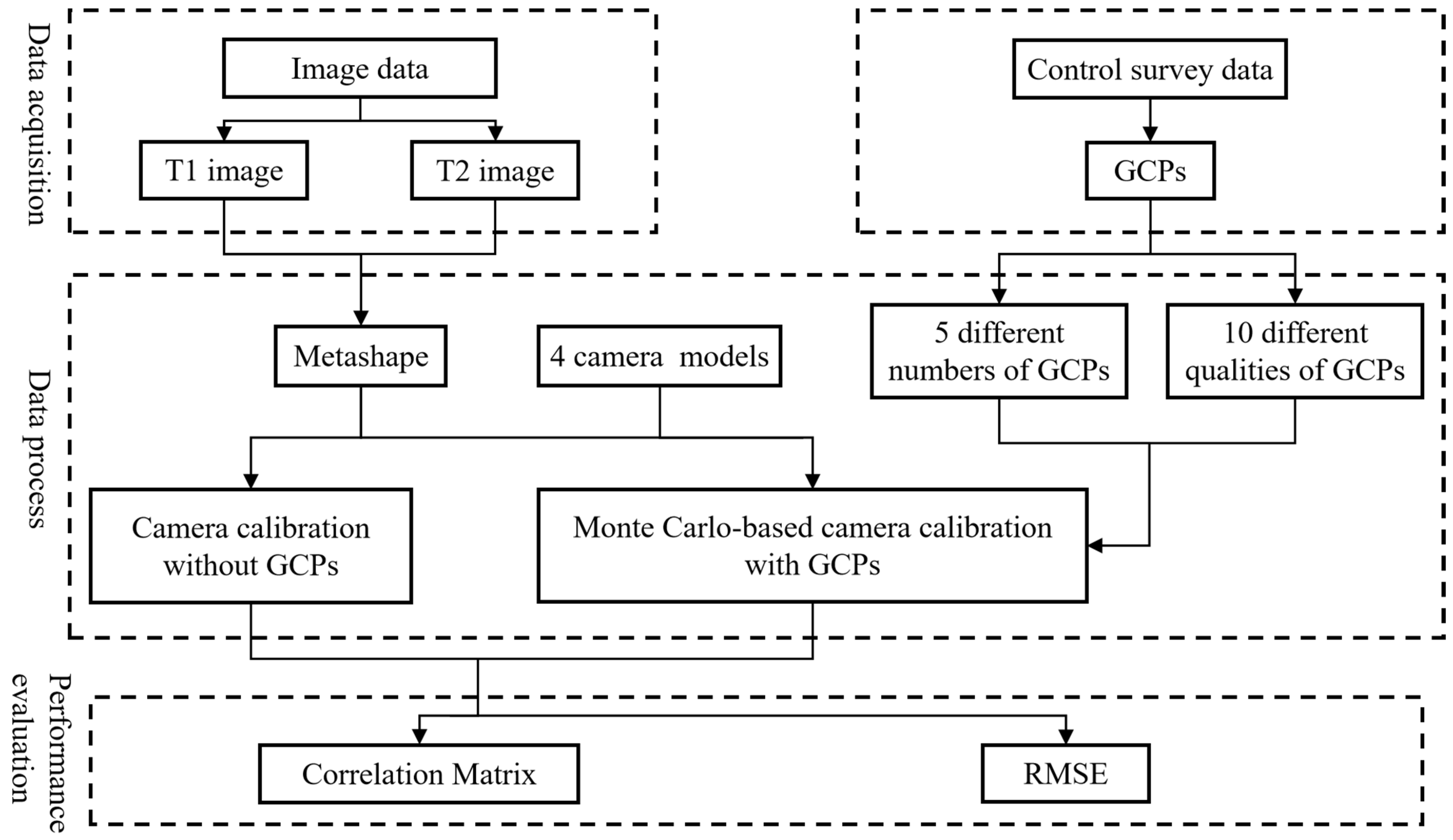
2. Methods
2.1. Basic Methods
2.2. Study Areas and Data
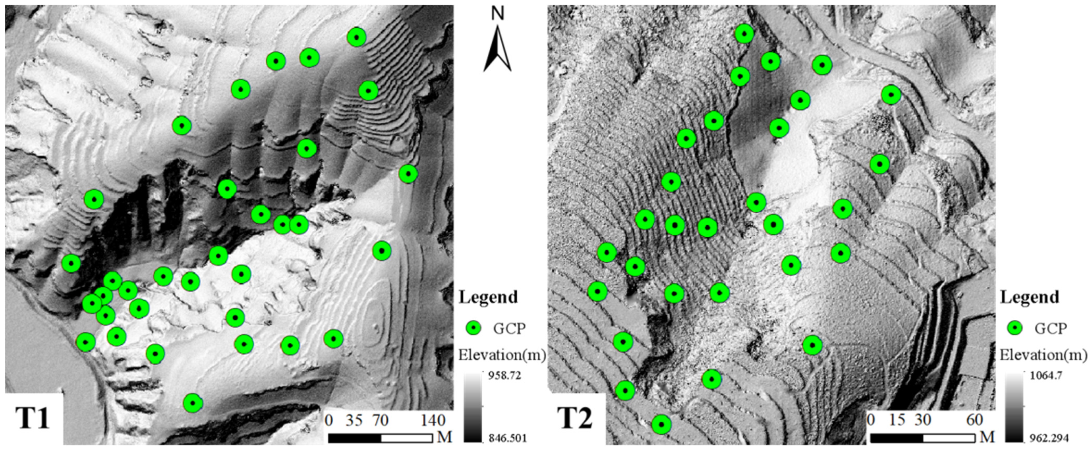
2.2.1. Study Areas
2.2.2. UAV Data Acquisition
- Image Data
- Control Survey Data
2.3. Camera Models
2.4. The Synergistic Effects of GCPs and Camera Models
2.4.1. Interaction Between the Number of GCPs and Camera Models
2.4.2. Interaction Between the Quality of GCPs and Camera Models
2.5. Performance Evaluation
3. Results
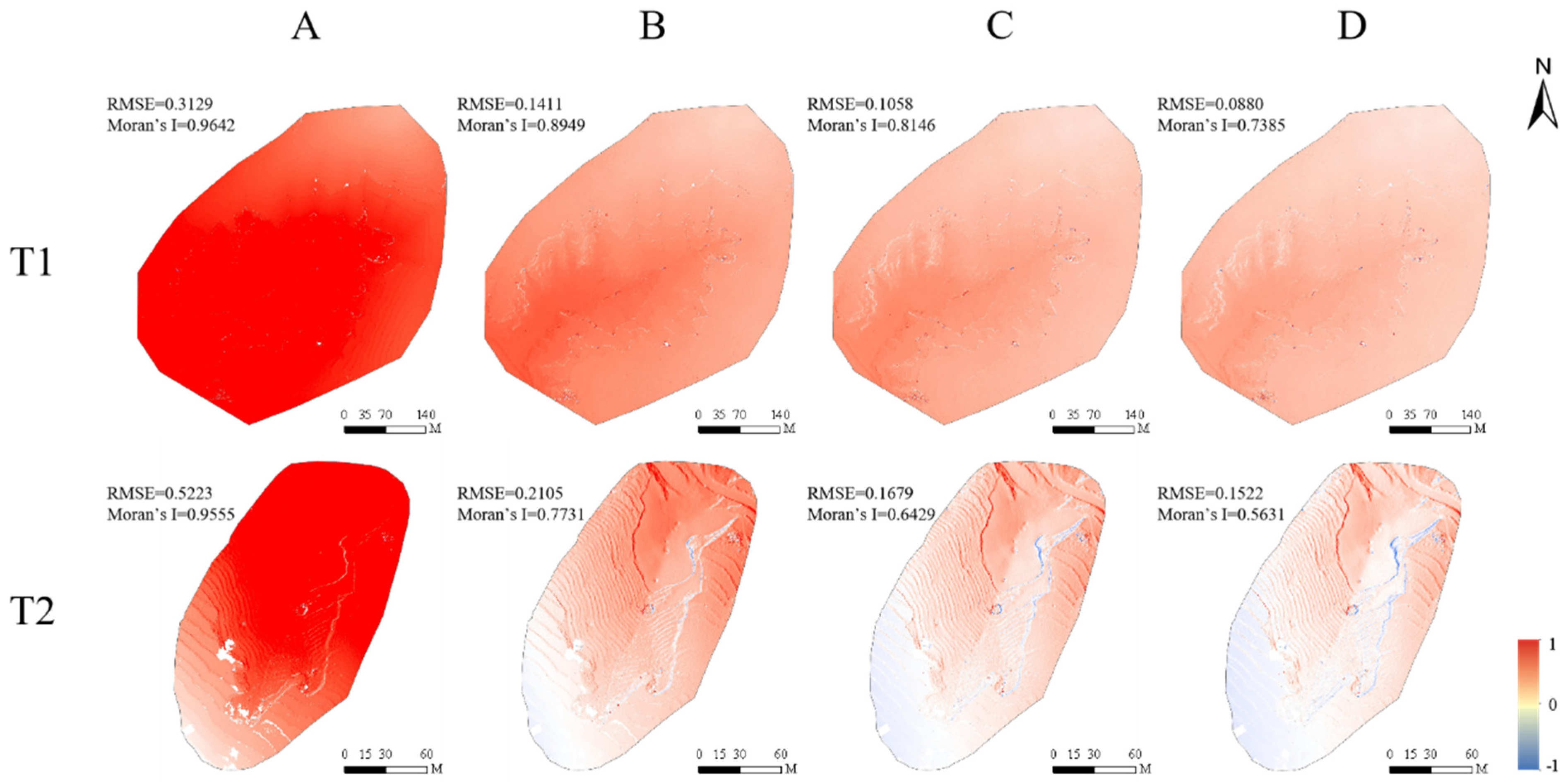
3.1. Effects of Camera Models
3.1.1. Camera Calibration Without GCPs
3.1.2. Effects of Camera Models on Terrain Modeling Accuracy
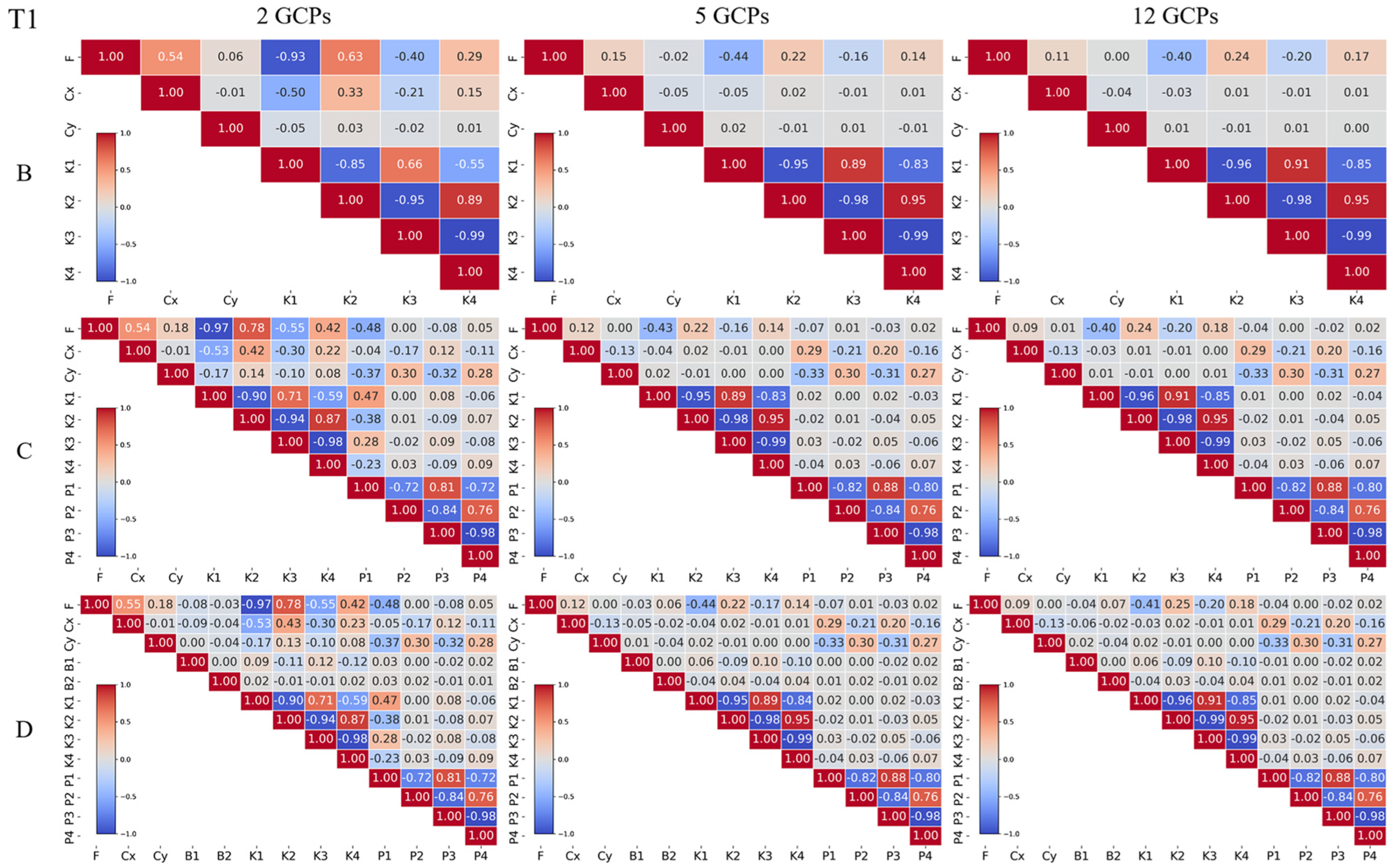
3.2. Interaction Between the Number of GCPs and Camera Models
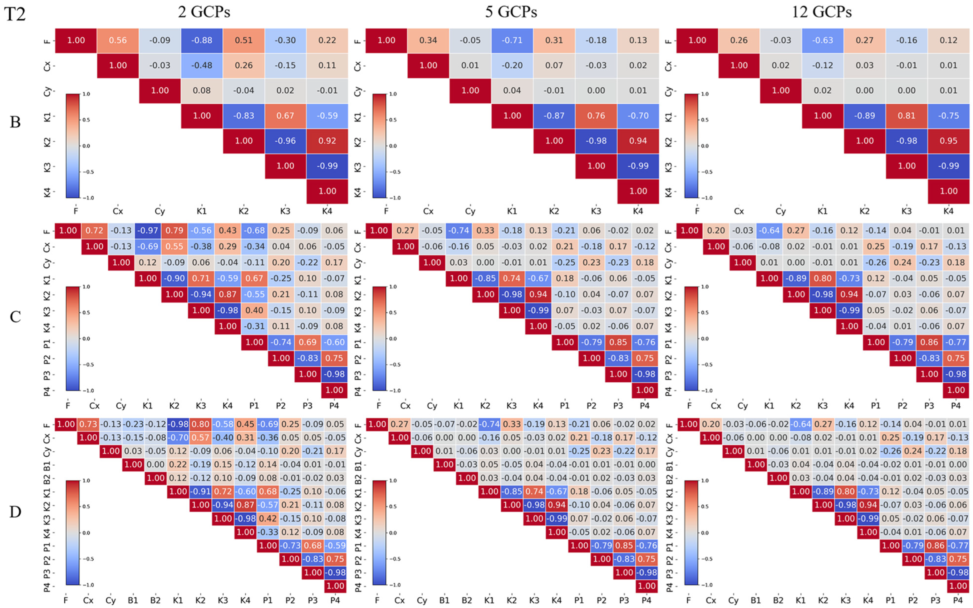
3.2.1. Effects of GCP Number on Camera Calibration
3.2.2. Interaction Effects on Terrain Modeling Accuracy
3.3. Interaction Between the Quality of GCPs and Camera Models
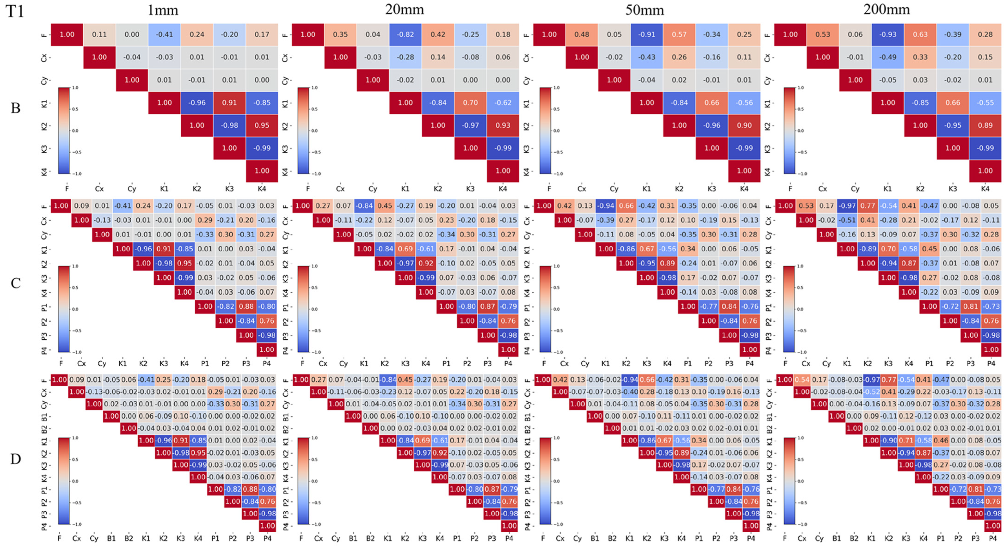
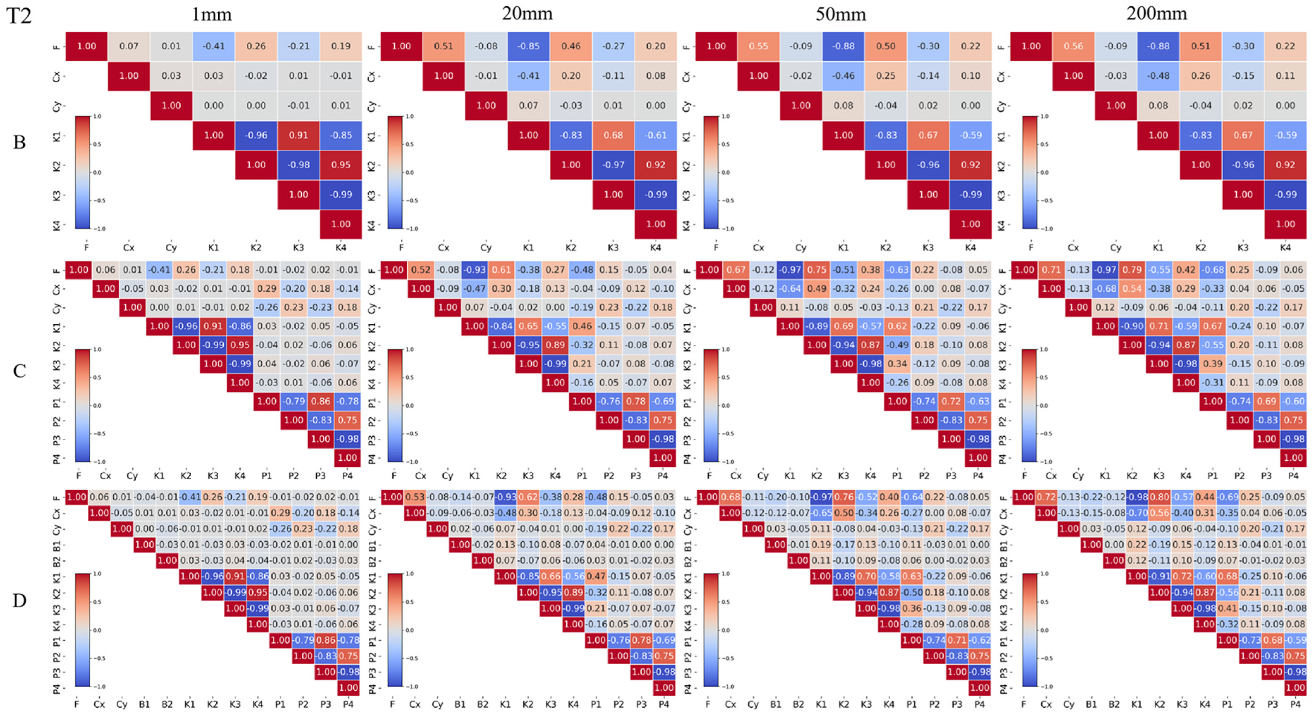
3.3.1. Effects of GCP Quality on Camera Calibration
3.3.2. Interaction Effects on Terrain Modeling Accuracy
4. Discussion
4.1. Camera Model Selection Strategy
4.2. Interaction Between the Number of GCPs and Camera Models
4.3. Interaction Between the Quality of GCPs and Camera Models
5. Conclusions
- Without GCPs, camera model selection is critical for improving camera calibration and terrain modeling accuracy. The use of complex camera models can reduce the overall correlation between distortion parameters. Compared with the simple model such as Model A (with only distortion parameter F), complex camera models can improve terrain modeling accuracy by approximately 70% and mitigate the spatial correlation. Model C (with F, Cx, Cy, K1–K4, and P1–P4) achieves a balance between camera model complexity and accuracy, making it a practical choice for most applications.
- When GCPs are available, the number of GCPs has a more significant effect on the accuracy improvement than the camera models. Increasing the number of GCPs can reduce the correlation between distortion parameters and improve the performance of camera models, thus improving the terrain modeling accuracy by approximately 45% to 70%. At the same time, the camera model complexity does not influence the required number of GCPs.
- When the GCP number is fixed, an interaction exists between the quality of GCPs and camera model selection. High-quality GCPs effectively mitigate the correlation between distortion parameters, leading to enhancing camera calibration and terrain modeling accuracy, with the RMSE of complex camera models decreasing by approximately 45% to 65%. Meanwhile, on the premise of ensuring effective calibration, complex camera models reduce the requirement for GCP quality. In other words, a more complex camera model should be chosen when the GCP quality is low.
Author Contributions
Funding
Data Availability Statement
Acknowledgments
Conflicts of Interest
References
- Pierzchała, M.; Talbot, B.; Astrup, R. Estimating Soil Displacement from Timber Extraction Trails in Steep Terrain: Application of an Unmanned Aircraft for 3D Modelling. Forests 2014, 5, 1212–1223. [Google Scholar] [CrossRef]
- Shahbazi, M.; Ménard, P.; Sohn, G.; Théau, J. Unmanned aerial image dataset: Ready for 3D reconstruction. Data Brief 2019, 25, 103962. [Google Scholar] [CrossRef] [PubMed]
- Chen, C.; Tian, B.; Wu, W.; Duan, Y.; Zhou, Y.; Zhang, C. UAV Photogrammetry in Intertidal Mudflats: Accuracy, Efficiency, and Potential for Integration with Satellite Imagery. Remote Sens. 2023, 15, 1814. [Google Scholar] [CrossRef]
- Gonçalves, J.A.; Henriques, R. UAV photogrammetry for topographic monitoring of coastal areas. ISPRS J. Photogramm. Remote Sens. 2015, 104, 101–111. [Google Scholar] [CrossRef]
- Manfreda, S.; McCabe, M.F.; Miller, P.E.; Lucas, R.; Pajuelo Madrigal, V.; Mallinis, G.; Ben Dor, E.; Helman, D.; Estes, L.; Ciraolo, G.; et al. On the Use of Unmanned Aerial Systems for Environmental Monitoring. Remote Sens. 2018, 10, 641. [Google Scholar] [CrossRef]
- Jaud, M.; Bertin, S.; Beauverger, M.; Augereau, E.; Delacourt, C. RTK GNSS-Assisted Terrestrial SfM Photogrammetry without GCP: Application to Coastal Morphodynamics Monitoring. Remote Sens. 2020, 12, 1889. [Google Scholar] [CrossRef]
- Cao, L.; Liu, H.; Fu, X.; Zhang, Z.; Shen, X.; Ruan, H. Comparison of UAV LiDAR and Digital Aerial Photogrammetry Point Clouds for Estimating Forest Structural Attributes in Subtropical Planted Forests. Forests 2019, 10, 145. [Google Scholar] [CrossRef]
- Candiago, S.; Remondino, F.; De Giglio, M.; Dubbini, M.; Gattelli, M. Evaluating Multispectral Images and Vegetation Indices for Precision Farming Applications from UAV Images. Remote Sens. 2015, 7, 4026–4047. [Google Scholar] [CrossRef]
- Bendig, J.; Yu, K.; Aasen, H.; Bolten, A.; Bennertz, S.; Broscheit, J.; Gnyp, M.L.; Bareth, G. Combining UAV-based plant height from crop surface models, visible, and near infrared vegetation indices for biomass monitoring in barley. Int. J. Appl. Earth Obs. Geoinf. 2015, 39, 79–87. [Google Scholar] [CrossRef]
- Tu, Y.-H.; Phinn, S.; Johansen, K.; Robson, A.; Wu, D. Optimising drone flight planning for measuring horticultural tree crop structure. ISPRS J. Photogramm. Remote Sens. 2020, 160, 83–96. [Google Scholar] [CrossRef]
- Swayze, N.C.; Tinkham, W.T.; Vogeler, J.C.; Hudak, A.T. Influence of flight parameters on UAS-based monitoring of tree height, diameter, and density. Remote Sens. Environ. 2021, 263, 112540. [Google Scholar] [CrossRef]
- Kameyama, S.; Sugiura, K. Effects of Differences in Structure from Motion Software on Image Processing of Unmanned Aerial Vehicle Photography and Estimation of Crown Area and Tree Height in Forests. Remote Sens. 2021, 13, 626. [Google Scholar] [CrossRef]
- Zhao, N.; Lu, W.; Sheng, M.; Chen, Y.; Tang, J.; Yu, F.R.; Wong, K.K. UAV-Assisted Emergency Networks in Disasters. IEEE Wireless Commun. 2019, 26, 45–51. [Google Scholar] [CrossRef]
- Erdelj, M.; Natalizio, E.; Chowdhury, K.R.; Akyildiz, I.F. Help from the Sky: Leveraging UAVs for Disaster Management. IEEE Pervasive Comput. 2017, 16, 24–32. [Google Scholar] [CrossRef]
- Tuna, G.; Nefzi, B.; Conte, G. Unmanned aerial vehicle-aided communications system for disaster recovery. J. Netw. Comput. Appl. 2014, 41, 27–36. [Google Scholar] [CrossRef]
- Templin, T.; Popielarczyk, D.; Kosecki, R. Application of Low-Cost Fixed-Wing UAV for Inland Lakes Shoreline Investigation. Pure Appl. Geophys. 2018, 175, 3263–3283. [Google Scholar] [CrossRef]
- Luhmann, T.; Fraser, C.; Maas, H.-G. Sensor modelling and camera calibration for close-range photogrammetry. ISPRS J. Photogramm. Remote Sens. 2016, 115, 37–46. [Google Scholar] [CrossRef]
- Zhang, Z. A flexible new technique for camera calibration. IEEE Trans. Pattern Anal. Mach. Intell. 2000, 22, 1330–1334. [Google Scholar] [CrossRef]
- Zhou, Y.; Rupnik, E.; Meynard, C.; Thom, C.; Pierrot-Deseilligny, M. Simulation and Analysis of Photogrammetric UAV Image Blocks—Influence of Camera Calibration Error. Remote Sens. 2020, 12, 22. [Google Scholar] [CrossRef]
- Jiménez-Jiménez, S.I.; Ojeda-Bustamante, W.; Marcial-Pablo, M.d.J.; Enciso, J. Digital Terrain Models Generated with Low-Cost UAV Photogrammetry: Methodology and Accuracy. ISPRS Int. J. Geo-Inf. 2021, 10, 285. [Google Scholar] [CrossRef]
- Weng, J.; Cohen, P.; Herniou, M. Camera calibration with distortion models and accuracy evaluation. IEEE Trans. Pattern Anal. Mach. Intell. 1992, 14, 965–980. [Google Scholar] [CrossRef]
- Samper, D.; Santolaria, J.; Majarena, A.C.; Aguilar, J.J. Comprehensive simulation software for teaching camera calibration by a constructivist methodology. Measurement 2010, 43, 618–630. [Google Scholar] [CrossRef]
- Basu, A.; Licardie, S. Alternative models for fish-eye lenses. Pattern Recognit. Lett. 1995, 16, 433–441. [Google Scholar] [CrossRef]
- Devernay, F.; Faugeras, O. Straight lines have to be straight. Mach. Vision Appl. 2001, 13, 14–24. [Google Scholar] [CrossRef]
- Hartley, R.; Kang, S.B. Parameter-Free Radial Distortion Correction with Center of Distortion Estimation. IEEE Trans. Pattern Anal. Mach. Intell. 2007, 29, 1309–1321. [Google Scholar] [CrossRef]
- Claus, D.; Fitzgibbon, A.W. A rational function lens distortion model for general cameras. In Proceedings of the 2005 IEEE Computer Society Conference on Computer Vision and Pattern Recognition (CVPR’05), San Diego, CA, USA, 20–25 June 2005; pp. 213–219. [Google Scholar]
- Jaud, M.; Passot, S.; Allemand, P.; Le Dantec, N.; Grandjean, P.; Delacourt, C. Suggestions to Limit Geometric Distortions in the Reconstruction of Linear Coastal Landforms by SfM Photogrammetry with PhotoScan® and MicMac® for UAV Surveys with Restricted GCPs Pattern. Drones 2019, 3, 2. [Google Scholar] [CrossRef]
- Li, D. The Correlation Analysis of a Self-Calibrating Bundle Block Adjustment and the Test of Significance of Additional parameters. Geomat. Inf. Sci. Wuhan Univ. 1981, 6, 46–65. [Google Scholar] [CrossRef]
- Li, D. The Overcoming of the Overparametrization in Self-Calibrating Adjustment. Geomat. Inf. Sci. Wuhan Univ. 1986, 11, 95–104. [Google Scholar] [CrossRef]
- Obanawa, H.; Sakanoue, S. Conditions of Aerial Photography to Reduce Doming Effect. In Proceedings of the IGARSS 2020—2020 IEEE International Geoscience and Remote Sensing Symposium, Waikoloa, HI, USA, 26 September–2 October 2020; pp. 6464–6466. [Google Scholar]
- Carbonneau, P.E.; Dietrich, J.T. Cost-effective non-metric photogrammetry from consumer-grade sUAS: Implications for direct georeferencing of structure from motion photogrammetry. Earth Surf. Process. Landf. 2017, 42, 473–486. [Google Scholar] [CrossRef]
- James, M.R.; Antoniazza, G.; Robson, S.; Lane, S.N. Mitigating systematic error in topographic models for geomorphic change detection: Accuracy, precision and considerations beyond off-nadir imagery. Earth Surf. Process. Landf. 2020, 45, 2251–2271. [Google Scholar] [CrossRef]
- Xu, X.; Xu, A.; Ma, L.; Jiao, H. The Influence of Lens Distortion Parameters on Measurement Accuracy of Image Points in Aerial Photogrammetry. Bull. Surv. Map. 2017, 0, 30–34. [Google Scholar] [CrossRef]
- Dai, W.; Zheng, G.; Antoniazza, G.; Zhao, F.; Chen, K.; Lu, W.; Lane, S.N. Improving UAV-SfM photogrammetry for modelling high-relief terrain: Image collection strategies and ground control quantity. Earth Surf. Process. Landf. 2023, 48, 2884–2899. [Google Scholar] [CrossRef]
- Wang, L.; Liu, G. Three Camera Lens Distortion Correction Models and Its Application. In Proceedings of the 2022 3rd International Conference on Geology, Mapping and Remote Sensing (ICGMRS), Zhoushan, China, 22–24 April 2022; pp. 462–467. [Google Scholar]
- Santos Santana, L.; Araújo E Silva Ferraz, G.; Bedin Marin, D.; Dienevam Souza Barbosa, B.; Mendes Dos Santos, L.; Ferreira Ponciano Ferraz, P.; Conti, L.; Camiciottoli, S.; Rossi, G. Influence of flight altitude and control points in the georeferencing of images obtained by unmanned aerial vehicle. Eur. J. Remote Sens. 2021, 54, 59–71. [Google Scholar] [CrossRef]
- Whitehead, K.; Hugenholtz, C.H. Applying ASPRS Accuracy Standards to Surveys from Small Unmanned Aircraft Systems (UAS). Photogramm. Eng. Remote Sens. 2015, 81, 787–793. [Google Scholar] [CrossRef]
- Mancini, F.; Dubbini, M.; Gattelli, M.; Stecchi, F.; Fabbri, S.; Gabbianelli, G. Using Unmanned Aerial Vehicles (UAV) for High-Resolution Reconstruction of Topography: The Structure from Motion Approach on Coastal Environments. Remote Sens. 2013, 5, 6880–6898. [Google Scholar] [CrossRef]
- Liu, X.; Lian, X.; Yang, W.; Wang, F.; Han, Y.; Zhang, Y. Accuracy Assessment of a UAV Direct Georeferencing Method and Impact of the Configuration of Ground Control Points. Drones 2022, 6, 30. [Google Scholar] [CrossRef]
- James, M.R.; Robson, S.; d’Oleire-Oltmanns, S.; Niethammer, U. Optimising UAV topographic surveys processed with structure-from-motion: Ground control quality, quantity and bundle adjustment. Geomorphology 2017, 280, 51–66. [Google Scholar] [CrossRef]
- Moran, P.A.P. Notes on Continuous Stochastic Phenomena. Biometrika 1950, 37, 17–23. [Google Scholar] [CrossRef]
- James, M.R.; Robson, S.; Smith, M.W. 3-D uncertainty-based topographic change detection with structure-from-motion photogrammetry: Precision maps for ground control and directly georeferenced surveys. Earth Surf. Processes Landf. 2017, 42, 1769–1788. [Google Scholar] [CrossRef]
- Sadeq, H.A. Accuracy assessment using different UAV image overlaps. J. Unmanned Veh. Syst. 2019, 7, 175–193. [Google Scholar] [CrossRef]
- Torres-Sánchez, J.; López-Granados, F.; Borra-Serrano, I.; Peña, J.M. Assessing UAV-collected image overlap influence on computation time and digital surface model accuracy in olive orchards. Precis. Agric. 2018, 19, 115–133. [Google Scholar] [CrossRef]
- Domingo, D.; Ørka, H.O.; Næsset, E.; Kachamba, D.; Gobakken, T. Effects of UAV Image Resolution, Camera Type, and Image Overlap on Accuracy of Biomass Predictions in a Tropical Woodland. Remote Sens. 2019, 11, 948. [Google Scholar] [CrossRef]
- You, Z.; Luan, Z.; Wei, X. General lens distortion model expressed by image pixel coordinate. Opt. Tech. 2015, 41, 265–269. [Google Scholar] [CrossRef]
- Fitzgibbon, A.W. Simultaneous linear estimation of multiple view geometry and lens distortion. In Proceedings of the 2001 IEEE Computer Society Conference on Computer Vision and Pattern Recognition. CVPR 2001, Kauai, HI, USA, 8–14 December 2001; p. I. [Google Scholar]
- Wang, J.; Shi, F.; Zhang, J.; Liu, Y. A new calibration model of camera lens distortion. Pattern Recognit. 2008, 41, 607–615. [Google Scholar] [CrossRef]
- Fraser, C.S. Automatic Camera Calibration in Close Range Photogrammetry. Photogramm. Eng. Remote Sens. 2013, 79, 381–388. [Google Scholar] [CrossRef]
- Dai, W.; Qiu, R.; Wang, B.; Lu, W.; Zheng, G.; Amankwah, S.O.Y.; Wang, G. Enhancing UAV-SfM Photogrammetry for Terrain Modeling from the Perspective of Spatial Structure of Errors. Remote Sens. 2023, 15, 4305. [Google Scholar] [CrossRef]
- De Marco, J.; Maset, E.; Cucchiaro, S.; Beinat, A.; Cazorzi, F. Remote SensingAssessing Repeatability and Reproducibility of Structure-from-Motion Photogrammetry for 3D Terrain Mapping of Riverbeds. Remote Sens. 2021, 13, 2572. [Google Scholar] [CrossRef]
- Atik, M.E.; Arkali, M. Comparative Assessment of the Effect of Positioning Techniques and Ground Control Point Distribution Models on the Accuracy of UAV-Based Photogrammetric Production. Drones 2025, 9, 15. [Google Scholar] [CrossRef]


| Parameters | Focal Length (F) | Principal Point (Cx, Cy) | Radial Distortion (K1, K2, K3, K4) | Tangential Distortion (P1, P2, P3, P4) | Aspect Ratio and Skew (B1, B2) | |
|---|---|---|---|---|---|---|
| Camera Model | ||||||
| A | ✓ | |||||
| B | ✓ | ✓ | ✓ | |||
| C | ✓ | ✓ | ✓ | ✓ | ||
| D | ✓ | ✓ | ✓ | ✓ | ✓ | |
Disclaimer/Publisher’s Note: The statements, opinions and data contained in all publications are solely those of the individual author(s) and contributor(s) and not of MDPI and/or the editor(s). MDPI and/or the editor(s) disclaim responsibility for any injury to people or property resulting from any ideas, methods, instructions or products referred to in the content. |
© 2025 by the authors. Licensee MDPI, Basel, Switzerland. This article is an open access article distributed under the terms and conditions of the Creative Commons Attribution (CC BY) license (https://creativecommons.org/licenses/by/4.0/).
Share and Cite
Wang, Z.; Shi, L.; Li, J.; Dai, W.; Lu, W.; Li, M. The Synergistic Effects of GCPs and Camera Calibration Models on UAV-SfM Photogrammetry. Drones 2025, 9, 343. https://doi.org/10.3390/drones9050343
Wang Z, Shi L, Li J, Dai W, Lu W, Li M. The Synergistic Effects of GCPs and Camera Calibration Models on UAV-SfM Photogrammetry. Drones. 2025; 9(5):343. https://doi.org/10.3390/drones9050343
Chicago/Turabian StyleWang, Zixin, Leyan Shi, Jinzhou Li, Wen Dai, Wangda Lu, and Mengqi Li. 2025. "The Synergistic Effects of GCPs and Camera Calibration Models on UAV-SfM Photogrammetry" Drones 9, no. 5: 343. https://doi.org/10.3390/drones9050343
APA StyleWang, Z., Shi, L., Li, J., Dai, W., Lu, W., & Li, M. (2025). The Synergistic Effects of GCPs and Camera Calibration Models on UAV-SfM Photogrammetry. Drones, 9(5), 343. https://doi.org/10.3390/drones9050343