Three-Dimensional Defect Measurement and Analysis of Wind Turbine Blades Using Unmanned Aerial Vehicles

Abstract

Wind turbines’ volume and power generation capacity have increased worldwide. Consequently, their inspection, maintenance, and repair are garnering increasing attention. Structural defects are common in turbine blades, but their detection is difficult due to the relatively large size of the blades. Therefore, engineers often use nondestructive testing. This study employed an unmanned aerial vehicle (UAV) to simultaneously capture visible-light and infrared thermal images of wind power blades. Subsequently, instant neural graphic primitives and neural radiance fields were used to reconstruct the visible-light image in three dimensions (3D) and generate a 3D mesh model. Experiments determined that after converting parts of the orthographic-view images to elevation- and depression-angle images, the success rate of camera attitude calculation increased from 85.6% to 97.4%. For defect measurement, the system first filters out the perspective images that account for 6–12% of the thermal image foreground area, thereby excluding most perspective images that are difficult to analyze. Based on the thermal image data of wind power generation blades, the blade was considered to be in a normal state when the full range, average value, and standard deviation of the relative temperature grayscale value in the foreground area were within their normal ranges. Otherwise, it was classified as abnormal. A heat accumulation percentage map was established from the perspective image of the abnormal state, and defect detection was based on the occurrence of local minima. When a defect was observed in the thermal image, the previously reconstructed 3D image was switched to the corresponding viewing angle to confirm the actual location of the defect on the blade. Thus, the proposed 3D image reconstruction process and thermal image quality analysis method are effective for the long-term monitoring of wind turbine blade quality.

1. Introduction

The volume and power generation capacity of wind turbines are increasing annually. During the operation of wind turbines, damage may occur over a long period, owing to environmental factors such as storms, heavy rains, high temperatures, and harsh sunlight. In addition to affecting the operating efficiency and decreasing power generation, damage can occur even if the defects are minor. Failure to detect them may lead to worsening of conditions. Among the various structural defects in wind turbines, blade defects are the most common [1,2,3]. Most of these defects are caused by manufacturing errors, such as imperfectly welded bonding joints. Under these conditions, the operation becomes prone to cracking or delamination. However, wind turbine blades are relatively large and complex to dismantle and inspect without damage. Therefore, nondestructive inspection methods are required, including visual [1,2,3,4,5,6], acoustic [7,8,9], vibration [10,11,12], and infrared (IR) thermal image detection [13,14,15,16].

Among these detection methods, visual inspection [1,2,3,4,5,6] of wind turbine blades offers advantages such as non-contact measurement, high efficiency, and a high degree of automation. However, it also faces limitations, including sensitivity to lighting conditions, camera angles, and background noise. Additionally, detecting internal damage or fine cracks remains challenging, requiring the integration of multimodal sensing technologies to enhance reliability. Acoustic [7,8,9] and vibration-based [10,11,12] methods typically require the installation of specialized sensors on wind turbine components. While effective for detecting structural anomalies, these approaches rely on long-term data collection to accurately analyze and predict faults. Moreover, surface-level issues such as paint peeling or minor blade damage are not readily identifiable in real time, limiting the effectiveness of early warning and preventive maintenance strategies. In addition, it is highly dangerous for operators to use machine tools while suspended for wind turbine inspections. In recent years, unmanned aerial vehicles (UAVs) have become common in military applications; geodetic observation; disaster relief; and inspection of bridges, wind power systems, and solar panels [17,18,19,20,21,22]. Therefore, UAVs can visually inspect wind turbine blades and capture visible-light images to observe surface damage.

Zhang et al. [5] proposed SOD-YOLO, a small target defect detection algorithm for wind turbine blades. After establishing a blade defect dataset using image foreground segmentation and Hough transform, they used an enhanced YOLOv5 that integrated a microscale detection layer and a lightweight structure for training. Similarly, Wu et al. [6] proposed a high-precision, YOLOv8-based approach that integrates a PC-EMA module for efficient surface defect detection in wind turbines while reducing model complexity. However, in their study, the inspection area was limited to the camera’s shooting range. Judging the shooting range on the blade solely from a partial image of the damaged location of the blade is challenging. Moreover, it can only detect surface defects and not internal defects.

IR thermal imaging can observe internal structural defects based on the surface temperature distribution in the shooting range. For example, Sanati et al. [14] developed thermal imaging technology that employs active and passive imaging methods and applied image processing technology to improve thermal contrast for internal defect detection in wind turbine blades. For the first time, step thermal imaging was applied to passive thermal imaging to improve internal defect visibility and the signal-to-noise ratio (SNR). In addition, Collider et al. [15] proposed a combination of thermal imaging and RGB data for wind turbine blade defect detection, a dataset containing 1000 fused images, and a deep learning model (such as DenseNet) for analysis. DenseNet exhibited accurate defect detection while optimizing feature extraction, reducing missed detection rates, and improving maintenance automation and accuracy. Reference [16] combined thermal imaging and computer vision for defect detection in wind turbine blades with large composite material structures, used the thermal characteristics generated by material friction for passive thermal imaging detection, and combined the principles of thermodynamics for damage location and assessment.

However, these studies focused on analyzing detailed defects and could not determine the actual location of defects in the wind turbine blade. Hence, three-dimensional (3D) reconstruction can be performed using multiview images to determine the position of the defect from every view corresponding to the 3D image. Several studies [23,24,25,26,27] have emphasized the advantages of image-based 3D reconstruction, such as precise camera pose estimation through triangulation and bundle adjustment, high-resolution modeling, and UAV compatibility. However, these methods are typically slower and computationally demanding and lack real-time capabilities. Although reliable and widely adopted, their limited processing speed and deployment flexibility reduce their effectiveness for large-scale or time-sensitive wind turbine monitoring tasks.

Mildenhall et al. [28] proposed the neural radiance field (NeRF), which learns the scene’s radiation and density fields from an image and its corresponding camera posture through a neural network (NN). Not only can they be visualized using ray tracing to synthesize hyper-realistic new perspective images, but they can also use the Marching Cubes algorithm [29] to generate a 3D grid model of the shooting scene from the density field. However, NeRF requires a long time to train, with each scene often taking hours or even days. To resolve this shortcoming, Müller et al. [30] proposed the instant neural graphic primitives (Instant NGP) method, which employs a multiresolution hash table of trainable feature parameters to replace the original input encoding of NeRF, resulting in a network model with a smaller structure and better results. The training time is considerably shortened through compute unified device architecture (CUDA)-based parallel computing on the GPU, and training can be completed in minutes or seconds.

Therefore, this study proposes a novel approach integrating UAV-mounted IR thermal imaging and advanced 3D reconstruction for wind turbine blade inspection. The method leverages the Instant NGP framework to achieve rapid and high-fidelity 3D reconstruction of the blade surface by capturing visible-light and thermal images from multiple viewpoints. Unlike traditional SfM-based techniques, Instant NGP significantly enhances processing speed and spatial detail. Thermal image analysis uses heat conduction theory [31] and statistical metrics [32] such as range, mean, and standard deviation, allowing for accurate defect characterization. Additionally, by mapping thermal image viewpoints onto their corresponding 3D views, the method is able to precisely locate defects in 3D models from multiple perspectives, thereby enhancing spatial awareness and inspection accuracy. This integrated framework addresses limitations in single-information image and defect localization seen in previous methods, offering an efficient, automated, and spatially accurate solution for wind turbine blade monitoring.

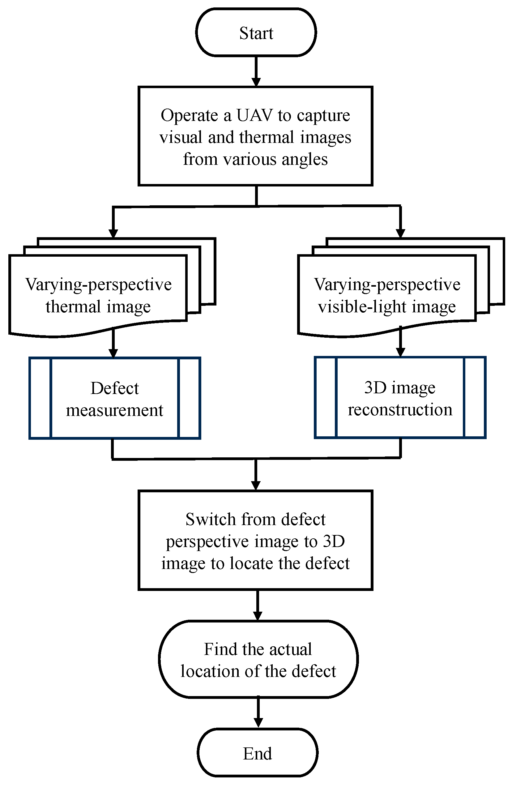
2. Sensing Method for Wind Turbine Blades

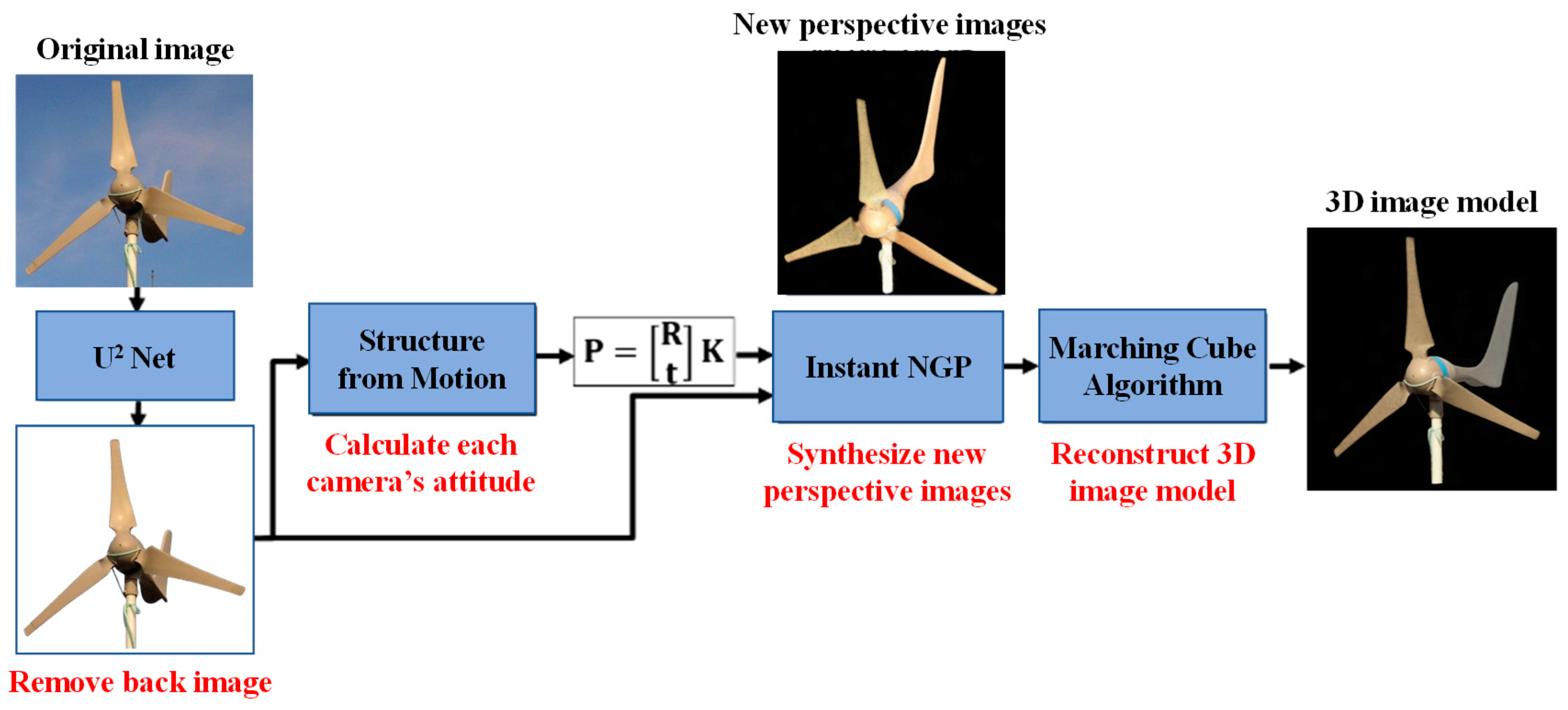
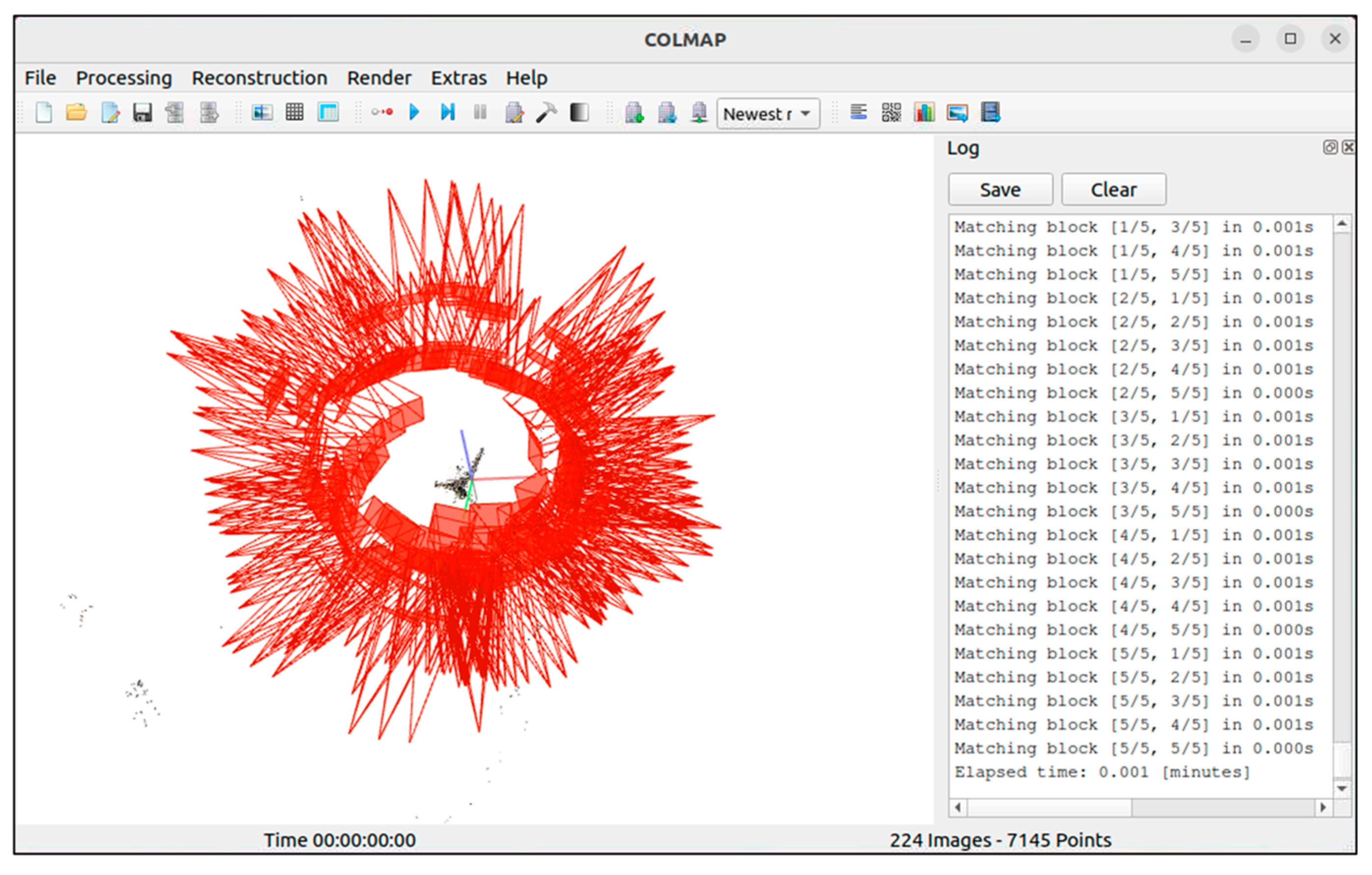
2.1. Three-Dimensional Reconstruction

The mathematical model of this study is based on theories and algorithms for the 3D reconstruction of visual images. Images of wind turbine blades were captured from various angles for the reconstruction. The reconstruction process is shown in Figure 1. The background of the original image is first removed through U² Net [33] to reduce the influence of background noise. The camera posture corresponding to each view in the image is calculated using the SfM algorithm. Both were used as inputs to the Instant NGP based on the NeRF network for 3D reconstruction. While reconstructing the 3D image, a 3D mesh model is generated using the marching cube algorithm. This section explains the fundamental theories and algorithms and presents theoretical derivations for the proposed reconstruction model.

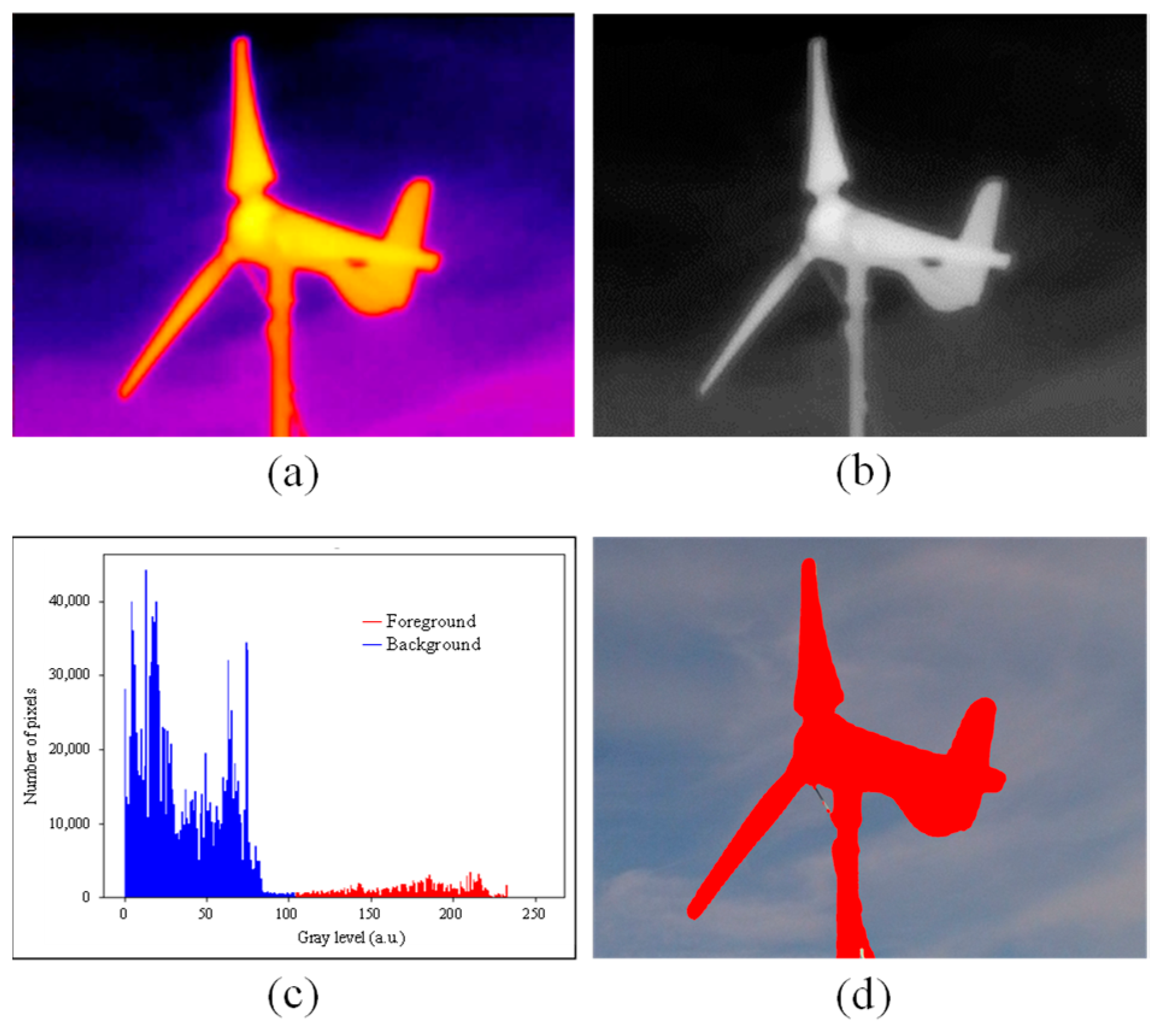
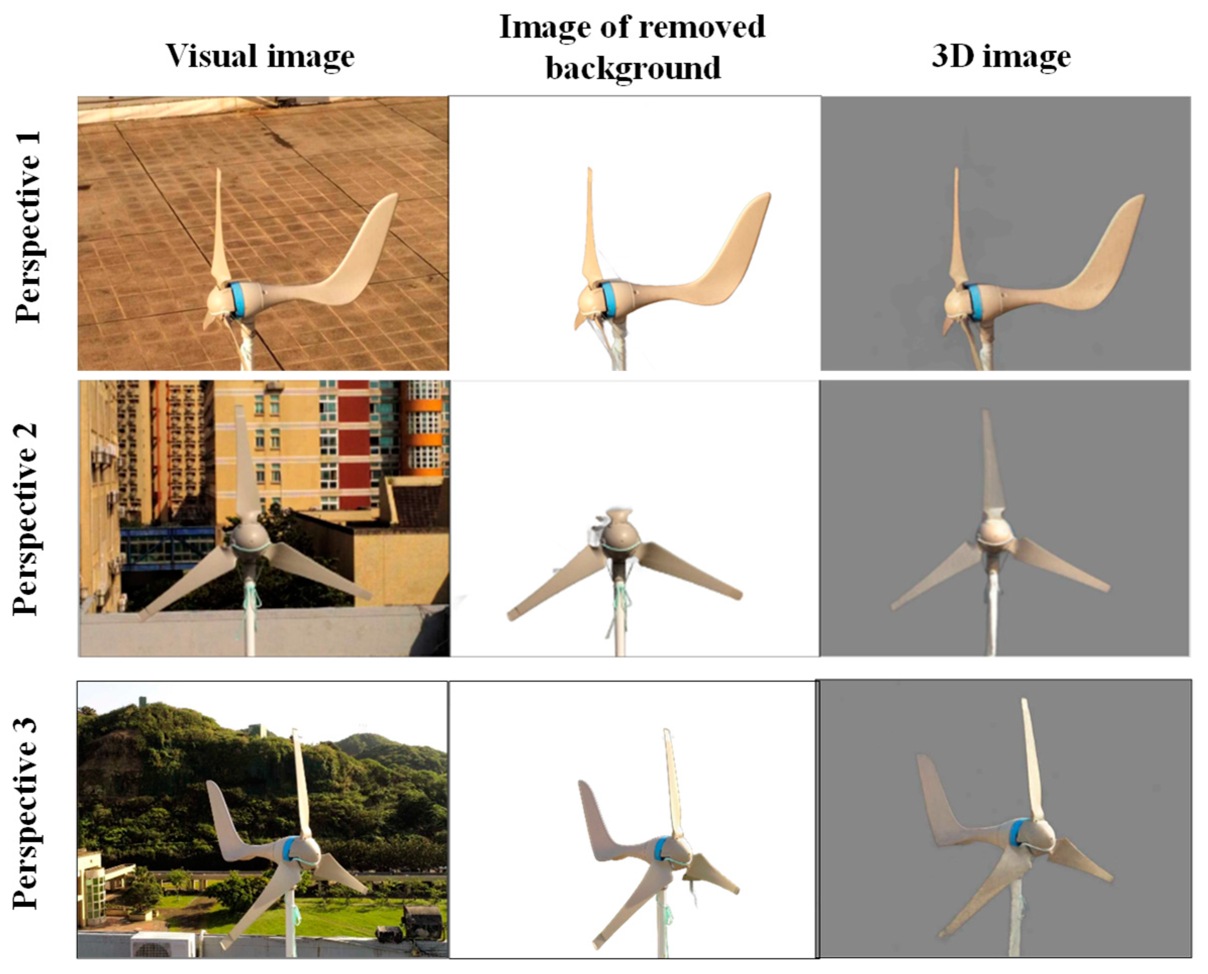
2.1.1. Removing Background Using the U² Net Method

Background interference is common when photographing wind turbines with a drone for 3D reconstruction. Therefore, this study employed U² Net [33], a two-level nested convolutional network composed of modules based on U-Net, to remove the background while preserving the wind turbine. To achieve high resolution, in the bottom layer, a ReSidual U (RSU) module was designed, which is able to extract intra-stage, multiscale features without reducing the resolution of feature maps; in the top layer, there is a U-Net-like structure in which an RSU module fills each stage. The structure of the RSU module is illustrated in Figure 2a. The image processing component uses salient object detection, which is compatible with various types of images and scenes. It can process complex images with details, blurred edges, or low contrast and generate high-definition images with quality segmentation results, making it an efficient, accurate, and facile method for effectively removing image backgrounds. The complete structure is shown in Figure 2b. The resolution of the feature map was progressively compressed and encoded into a high-resolution map to alleviate the loss of fine details when directly scaling up. Finally, masks were trained at each resolution after integrating the local and multiscale features. The masks were superimposed to form a foreground mask, retaining the foreground image while removing the background. This process reduced the influence of background debris, allowing the process to focus on turbine reconstruction.

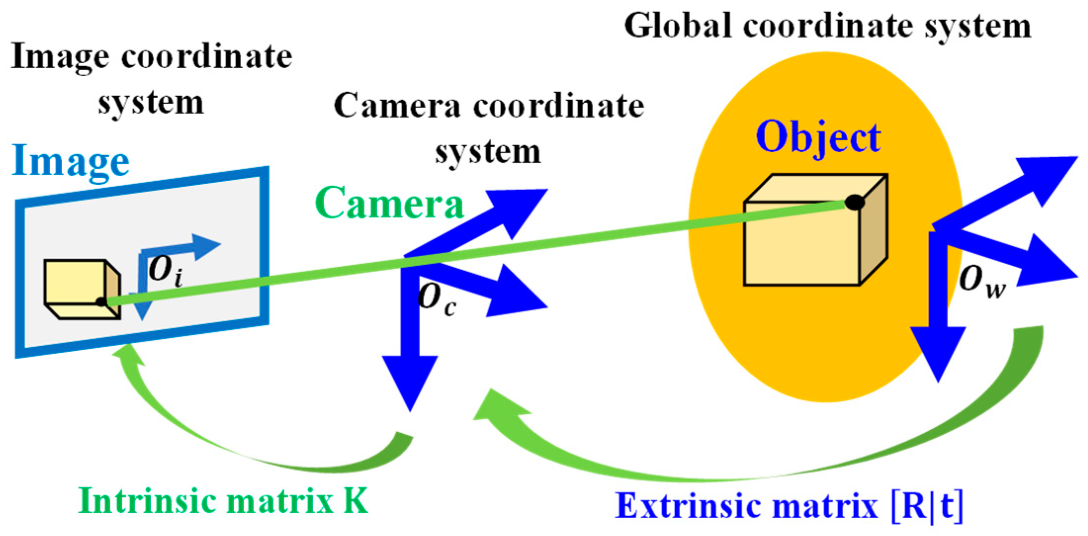
2.1.2. Coordinate Conversion of Camera Posture

In 3D reconstruction, the relative positions and angles of images from each perspective are key factors in drone photography. After mastering the camera posture for each image [23], we can simulate the image acquisition scenario in the subsequent algorithm and restore the structure of the shooting scene or object. The camera that captures the image should have an intrinsic matrix composed of camera parameters ($\mathbf{K}$). Each image has a corresponding camera matrix ($\mathbf{P}$), which is composed of $\mathbf{K}$ and the extrinsic matrix $\left[\mathbf{R}|\mathbf{t}\right]$ to be extrapolated to represent the camera posture when the camera captures the image. The relationships among the matrices in different coordinate systems are illustrated in Figure 3. When the camera shoots an image of a scene, the points on the object in the scene are converted from the global coordinate system to the camera coordinate system through the external orientation matrix. Subsequently, it is projected onto the image plane of the image’s image coordinate system through the inner orientation matrix.

Intrinsic Matrix

The intrinsic matrix ($\mathbf{K}$) [23] represents the geometric relationship between the photographic beam and imaging during image capture. It consists of several basic camera parameters, which are expressed as follows:

$$\mathbf{K}=\left[\begin{array}{ccc}{f}_x& 0& 0\\ s& f_y& 0\\ c_x& c_y& 1\end{array}\right],$$

(1)

where $\left(c_x , c_y\right)$ represent the image coordinates of the optical axis of the camera projected on the image; $\left(f_x , f_y\right)$ represents the focal length in pixels, obtained by dividing the focal length of the global unit length by the unit pixel length in the x and y directions, respectively; and $s$ is the skew coefficient, which is used to compensate for image distortion caused by tilting the camera lens.

Extrinsic Matrix

The extrinsic matrix [23] represents the geometric relationship between the object and the camera in the global and camera coordinate systems, which can be divided into a rotation matrix ($\mathbf{R}$) and translation vector ($\mathbf{t}$):

$$\left[\mathbf{R}|\mathbf{t}\right]=\left[\begin{array}{cccc}{r}_{11}& r_{12}& r_{13}& t_x\\ r_{21}& r_{22}& r_{23}& t_y\\ r_{31}& r_{32}& r_{33}& t_z\end{array}\right].$$

(2)

In 3D space, the rotation matrix ($\mathbf{R}$) can be calculated from the product of three two-dimensional (2D) rotation matrices at the respective rotation angles of the $\psi , \varphi , \theta$, x, y, and z axes:

$$\begin{array}{cc}\hfill \mathbf{R}& =R_x\left(\psi \right)R_y\left(\varphi \right)R_z\left(\theta \right)\hfill \\ & =\left[\begin{array}{ccc}\cos \psi \cos \theta & \sin \theta & -\sin \varphi \cos \theta \\ \sin \psi \sin \varphi \cos \theta -\cos \psi \sin \theta & \sin \psi \sin \varphi \sin \theta +\cos \psi \cos \theta & \sin \psi \cos \psi \\ \cos \psi \sin \varphi \cos \theta +\sin \psi \sin \theta & \cos \psi \sin \varphi \sin \theta -\sin \psi \cos \theta & \cos \psi \cos \varphi \end{array}\right]\hfill \\ & =\left[\begin{array}{ccc}{r}_{11}& r_{12}& r_{13}\\ r_{21}& r_{22}& r_{23}\\ r_{31}& r_{32}& r_{33}\end{array}\right],\hfill \end{array}$$

(3)

where $t_x$,$t_y$, and $t_z$ of the translation vector (t) are the translation components between the origins of the two coordinate systems in the x-, y-, and z-axis directions, respectively.

Camera Matrix

Each image has a corresponding camera matrix ($\mathbf{P}$), which represents the camera posture during image capture. According to the relationship between the inner and outer orientation matrices in the coordinate system, this matrix can be simplified as follows [23]:

$$\mathbf{P}=\mathbf{K}\left[\mathbf{R}|\mathbf{t}\right]=\left[\begin{array}{ccc}{f}_x& 0& 0\\ s& f_y& 0\\ c_x& c_y& 1\end{array}\right]\left[\begin{array}{cccc}{r}_{11}& r_{12}& r_{13}& t_x\\ r_{21}& r_{22}& r_{23}& t_y\\ r_{31}& r_{32}& r_{33}& t_z\end{array}\right],$$

(4)

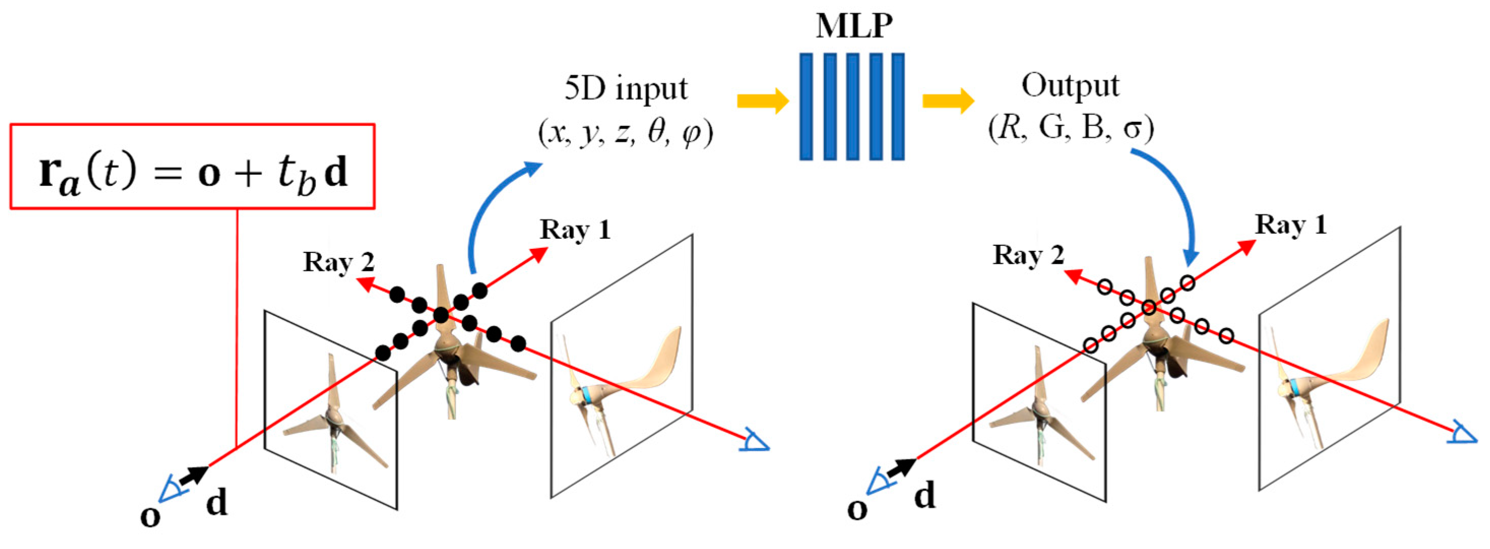
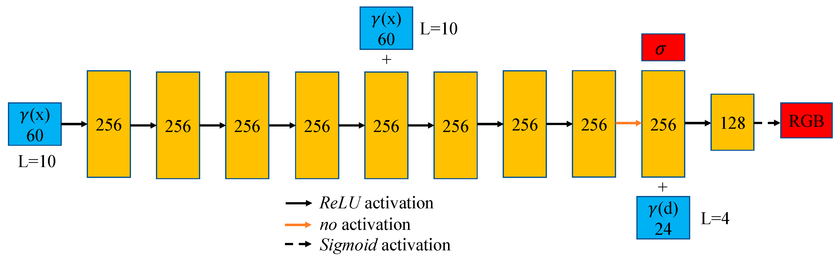
2.1.3. Image Process of Scene Radiation and Density Fields Using NeRF

According to the concept of ray tracing in computer graphics, when a camera captures an image of a scene, it can be simulated as a series of rays emitted from the perspective center of the camera to the scene through the image plane. The corresponding position on the ray determines the color of each pixel in the image. The result of information accumulated from the scene in the image plane can be divided into RGB values representing color and volume density ($\sigma$), which can be considered the probability of the ray stopping at the current position. The ray can be defined by the 3D coordinate vector of the camera’s perspective center ($\mathbf{o}$) and the unit direction vector of the ray emission ($\mathbf{d}$) as follows [28]:

$${\mathbf{r}}_{\mathit{a}}\left(t\right)=\mathbf{o}+t_b\mathbf{d}.$$

(5)

The scene is divided into 3D bounding boxes. Its radiation field and density field can be defined using two parameters corresponding to $\sigma \left({\mathbf{r}}_{\mathit{a}}\left(t_b\right)\right)$ for each 3D coordinate and $\mathrm{c}\left({\mathbf{r}}_{\mathit{a}}\left(t_b\right),\mathbf{d}\right)$ within the boundary. The RGB value ($C\left({\mathbf{r}}_{\mathit{a}}\right)$) accumulated by each ray in the pixel can be expressed as [28] follows:

$$C\left({\mathbf{r}}_{\mathit{a}}\right)={\int }_{{t_b}_n}^{{t_b}_f}T\left(t_b\right)\sigma \left({\mathbf{r}}_{\mathit{a}}\left(t_b\right)\right)\mathrm{c}\left({\mathbf{r}}_{\mathit{a}}\left(t_b\right),\mathbf{d}\right)d{t}_b,$$

(6)

where ${t_b}_n$ and ${t_b}_f$ represent the near and far bounds of the intersection of the ray, respectively. The bounding box and $T\left(t_b\right)$ are defined as follows [28]:

$$T\left(t_b\right)=exp\left(-{\int }_{{t_b}_n}^{{t_b}_f}\sigma \left({\mathbf{r}}_{\mathit{a}}\left(s\right)\right)d\mathrm{s}\right).$$

(7)

To optimize the training of NeRF, trigonometric function frequency encoding is used as the positional encoding of the NN input, considering that multilayer NNs have a poor ability to learn high-frequency functions [34,35]. This step enables the network to identify the location it is currently processing. For the network input (p), a combination of sine and cosine operations is used to project low-dimensional information onto a high-dimensional space. The formula is expressed as follows [28]:

$$\gamma \left(\mathbf{p}\right)=\left(\sin \left(2^0\pi \mathbf{p}\right), \cos \left(2^0\pi \mathbf{p}\right), \cdots , \sin \left(2^{\mathcal{l}-1}\pi \mathbf{p}\right), \cos \left(2^{\mathcal{l}-1}\pi \mathbf{p}\right) \right)$$

(8)

where $\mathcal{l}\in \mathbb{N}$ belongs to a set of experimental parameters that need to be adjusted to appropriate values based on the experimental results. The number of parameters input to the network through this formula is $2\mathcal{l}$. NeRF’s multilayer perceptron (MLP) input is a set of five-dimensional parameters, including 3D coordinates (x, y, z) and the two-dimensional parameters (θ, φ) representing the angle of the light emission direction. The output is the RGB value and volume density (σ) corresponding to the position. The operational process is depicted in Figure 4.

This study used the research results $(\mathrm{x},\mathrm{y},\mathrm{z})$ reported in [24] to define part of the input parameter as vector $\mathbf{x}$ and its experimental parameter ($\mathcal{l}$) as 10. The $(d_x,d_y,d_z)$ part in the input parameter is converted $(\theta ,\phi )$ into a unit direction vector ($\mathbf{d}$); then, its experimental parameter ($\mathcal{l}$) is set to 4. After using each input parameter for the NN through the position encoding of Equation (8), the number of parameters representing any position in space $\mathbf{x}$ increased from 3 to 60. The unit direction vector representing the ray direction ($\mathbf{d}$) increased from 3. The number of parameters increased to 24. The actual network structure of NeRF is illustrated in Figure 5. Position $\mathbf{x}$ was input into an 8-layer fully connected layer network with 256 neurons in the form of position encoding $\gamma \left(\mathbf{x}\right)$. The ReLU function was used as the excitation function in this process. Subsequently, the network structure of $\mathsf{\gamma }\left(\mathrm{x}\right)$ [36] was connected to the fifth layer of the fully connected layer network in the form of a skip connection. After adding a layer of the network to the output volume density ($\sigma$) and 256-dimensional feature vectors, the feature vectors were connected in series with ray angle $\gamma \left(\mathbf{d}\right)$. Finally, it was connected to a fully connected layer network with 128 neurons. The Sigmoid function was used as the excitation function to output $\mathbf{x}$ for the RGB value of the position in ray direction $\mathbf{d}$.

2.1.4. Optimizing the NeRF Network Structure Using the Instant NGP Method

Müller et al. [30] proposed a new input-encoding method and applied it to a series of NGP cases based on the NN training parameters. NeRF benefits from this technology; after replacing the original trigonometric function frequency encoding, the model can use a smaller NN-like structure to obtain equivalent or better results. The smaller network model and multiresolution hash encoding are processed in parallel on a GPU through CUDA, minimizing the training time significantly. This method reduces the training time to a few minutes or even seconds. The multiresolution hash coding process is illustrated in Figure 6. The resolution is first divided into $L$ different levels, including the integer coordinates ($x$) of the grid vertices of the input position. The hash function is expressed as follows:

$$h\left(x\right)=\left({\oplus }_{i=1}^{d_h} x_i{\pi }_i\right).$$

(9)

The corresponding hash value is then calculated and stored in a hash table, where $d_h=$ 3 represents the three dimensions of the input position coordinates, ${\pi }_1=1, {\pi }_2=2654435761$, and ${\pi }_3=805459861$. It is divided into $L$ resolution levels, and each resolution level has an $F$ feature vector with the maximum dimension ($T_h$) of the hash table. The feature vector corresponding to each vertex is retrieved from the hash table. The feature vector of the input position ($x$) is then calculated through interpolation. After repeating this process of encoding for each level of resolution, the various feature parameters and auxiliary parameters, such as the viewing-angle direction and texture ($\xi \in {\mathbb{R}}^E$), are concatenated together as the position encoding input $m\left(y;\mathsf{\Phi }\right)(y\in {\mathbb{R}}^{LF+E})$ of the NN.

2.1.5. Three-Dimensional Grid Model Generation Using the Marching Cube Algorithm

The marching cube algorithm [29] extracts isosurfaces from a 3D discrete data field and generates a 3D model. It is primarily used in the medical field for visualization, such as for 3D reconstruction of computed tomography and magnetic resonance imaging. The basic concept of this algorithm is to cut a 3D space into multiple cubes called voxels and use a set threshold (equivalent value) to determine whether it is a part of the model surface for the numerical value (eigenvalue) at the vertex of each cube. If the value on the voxel vertex is greater than or equal to the threshold, the vertex exists outside the isosurface and is marked as 0; conversely, if the value is less than the threshold, the vertex exists within the isosurface and is marked as 1. As each voxel unit has eight vertices, there are $2^8=256$ situations. Figure 7 illustrates the 15 basic polygon shapes of the marching cube algorithm. When a vertex is marked as zero, no marked point exists. When it is marked as 1, it is presented as a green-marked point. The remaining 241 forms can be obtained by rotating and mapping these 15 basic forms. Each voxel in the 3D space generates a polygon plane according to this method, and the intersection position of the polygon plane on the edge of the voxel is obtained by linear interpolation. Finally, a complete 3D mesh model is constructed by connecting all intersections.

This study’s density field obtained by training the NeRF was a 3D discrete data field. The 3D grid model of the shooting scene could be reconstructed using this algorithm. The color of the model is based on the radiation field, which determines the various angles of the shooting scene. The RGB value of the position is calculated by summing and averaging the values.

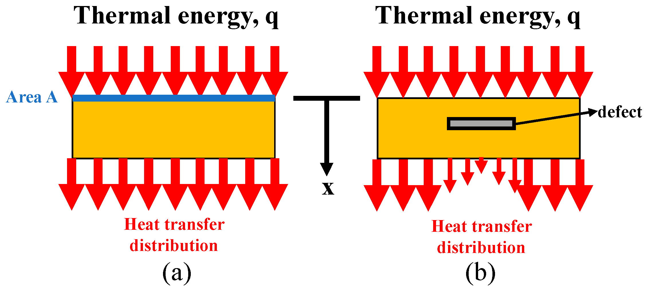
2.2. Heat Conduction Sensing

This study used thermal image sensing to measure the surface or internal defects in wind turbine blades. According to the heat conduction theory, drastic temperature gradients in surface temperature measurements result from surface or internal defects. Heat conduction occurs without significant material movement, primarily resulting from collisions and energy transfer between atoms or molecules. When there is a temperature gradient between objects or within one object, energy is transferred from high to low temperatures until thermal equilibrium is reached. Fourier’s law of heat conduction [31] describes this transfer process as follows:

$$q_x=-kA{\displaystyle \frac{\partial T}{\partial x}},$$

(10)

where $q_x$ represents heat transfer in the x-axis direction ($\mathrm{W}$), k represents the thermal conductivity coefficient of the object $\left(\mathrm{W}/\mathrm{m}·°\mathrm{C}\right)$, A represents the heat conduction cross-sectional area (${\mathrm{m}}^2$), T represents the temperature ($°\mathrm{C})$, ${\displaystyle \frac{\partial T}{\partial x}}$ represents the temperature gradient, and the negative sign represents the direction of heat conduction from high to low temperatures. According to this law, the heat conduction rate per unit area increases with the temperature gradient and is proportional to the thermal conductivity of the substance.

Whether air bubbles in the cracks or deterioration caused by factors such as rust, the defects in an object have different thermal conductivity coefficients due to the object itself, which results in different thermal energy transfer in different places. This causes a variable temperature distribution. Taking the heat conduction of a simple flat plate as an example (Figure 8), compared with a flat plate with a defect-free structure and a uniform heat conduction distribution, if the conduction coefficient at the defect is smaller, the flat plate transfers less heat to the defective structure. Consequently, the temperature is also lower, with local minima appearing in the IR thermal images. When the defect is thicker, the energy transfer becomes more evident. Therefore, thermal images and heat conduction theory can be used to detect defects in turbine fan blades. Finally, the scene corresponding to the 3D image at that angle of view is used to determine the camera’s shooting range and the location of the defect on the blade.

2.2.1. Thermal Image Analysis

The Anafi-USA UA can only use the relative temperature to generate color thermal images based on the color comparison table within the highest and lowest temperature ranges and within the image shooting range. Therefore, in this study, the grayscale value directly corresponds to the temperature after the captured thermal image was converted from a colored image into a grayscale image. A histogram was established from each grayscale value of the image. The horizontal axis represents grayscale values from 0 to 255, and the vertical axis represents the number of pixels computed using the grayscale value in the image. Otsu’s method [37] determines the optimal threshold from a grayscale image and divides the grayscale value into two intervals, representing the foreground and background, using the threshold as the boundary. This study’s foreground and background represent the turbine blades and the background, respectively. To determine the optimal threshold, the background part of the thermal image was filtered, and the area where the blades were located was analyzed (Figure 9). By converting the thermal image captured by the drone into a grayscale image, the pixel positions with a grayscale value higher than the threshold in the image can be summarized in the area with the blade, i.e., the red area.

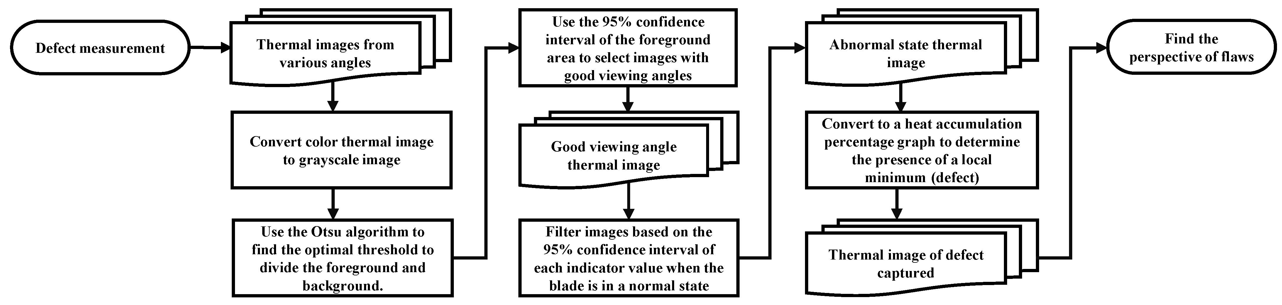
2.2.2. Defect Measurement of Wind Turbines

The complete wind turbine defect-measurement flow chart for this study is illustrated in Figure 10. Thermal images from multiple angles were first acquired using a UAV. These images were converted to grayscale, and the Otsu algorithm was applied to segment the foreground—defined as the blade area—from the background using the 95% confidence interval (CI) of the foreground region. To ensure quality analysis, images were initially filtered based on the proportion of the foreground area, selecting those with clear blade visibility as “good viewing-angle thermal images”. Subsequently, thermal images showing potential anomalies were identified as “abnormal-state thermal images” using the 95% CI of calculated statistical features. Finally, a heat accumulation percentage chart was used to visualize the temperature distribution, detect local minima as potential defects, and determine the optimal viewing angle for defect observation.

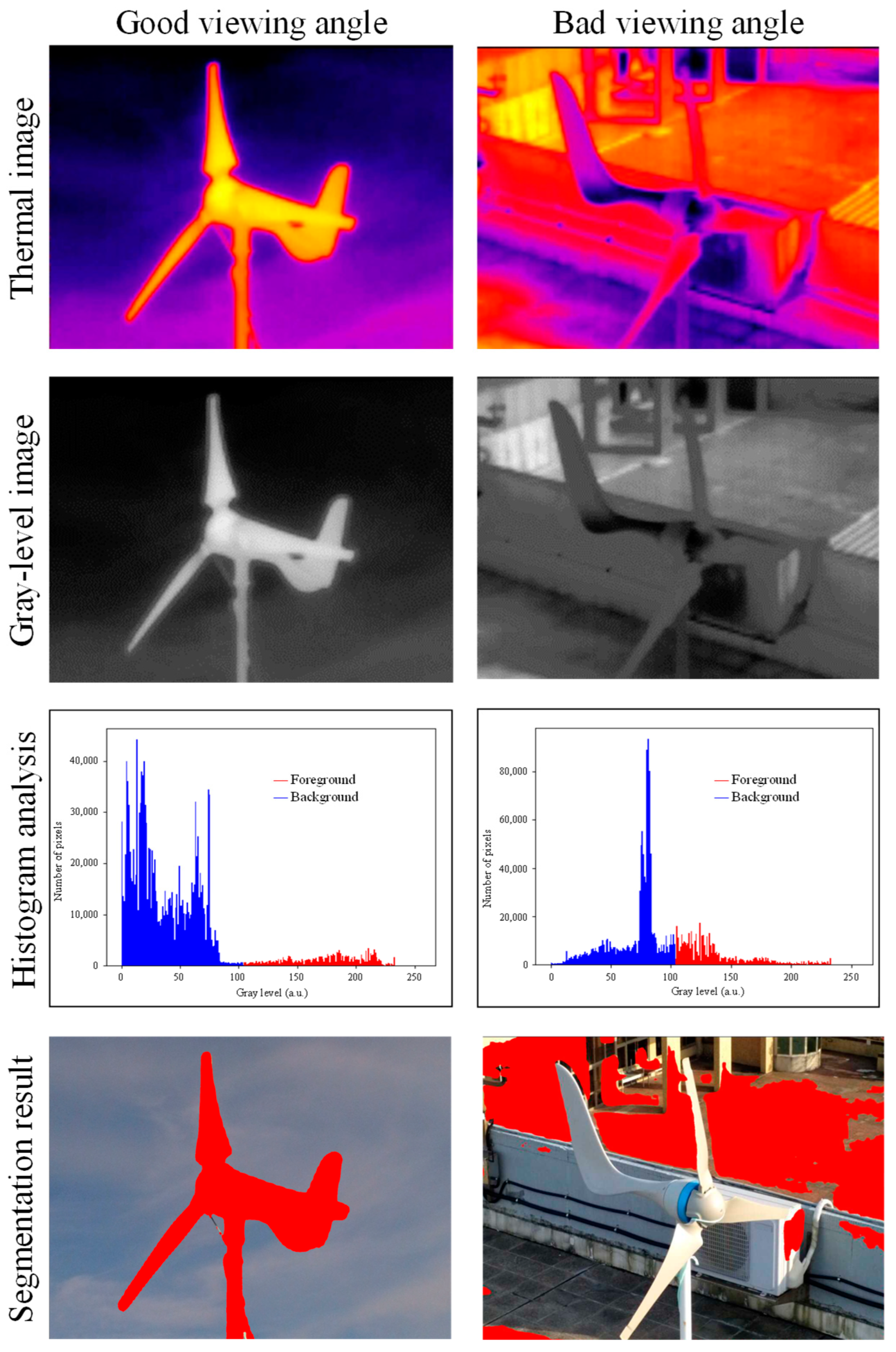
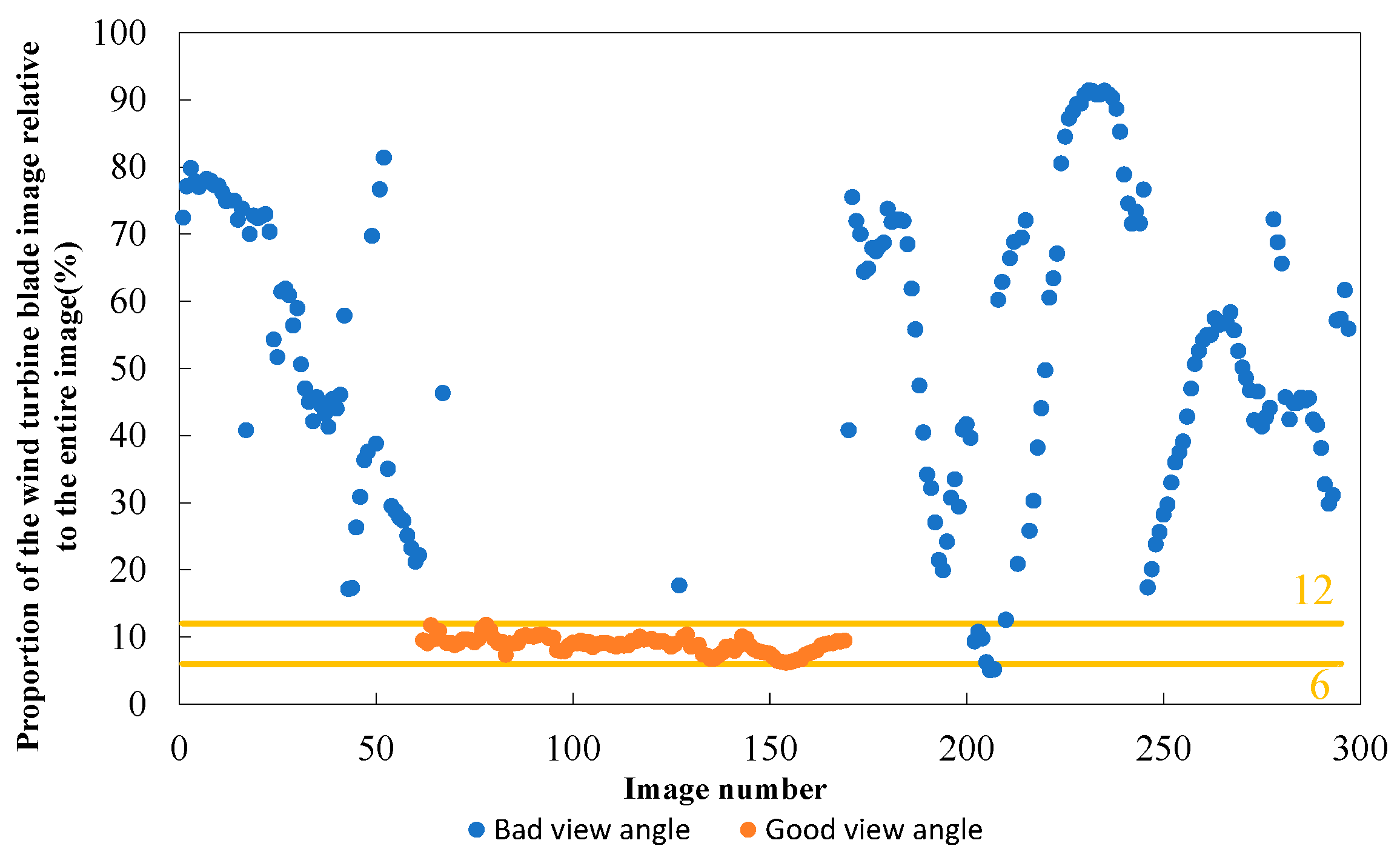
Good Viewing-Angle Image Screening

When shooting images from various viewing angles, the background may appear cluttered from certain viewing angles. In this case, separating the blade areas in the images from such viewing angles can be difficult. As illustrated in Figure 11, images captured from good viewing angles exhibit minimal background debris, making it easier to distinguish the blade region. The absence of clutter enhances the visibility of blade features, allowing defects to be more clearly identified. In contrast, poor viewing-angle images often contain excessive background noise, such as debris and shadows, which obscure the blade contours and hinder accurate segmentation. This interference can lead to incorrect defect detection and measurement. Therefore, selecting images with clear backgrounds and good viewing angles is essential to ensure reliable and precise defect analysis on the blades.

As illustrated in Figure 11, by observing the separation of the foreground and backgrounds of the images from various viewing angles, we can determine that most images captured from bad viewing angles with cluttered backgrounds conflate parts of the background, foreground, and the blades, causing the foreground to cover a larger area. Therefore, all good viewing-angle images were used to calculate the optimal threshold using Otsu’s algorithm, followed by determination of the pixel positions in the image with grayscale values higher than the threshold. After counting the number of pixels, the proportion of the foreground area can be calculated as follows:

$$\mathrm{F}\mathrm{o}\mathrm{r}\mathrm{e}\mathrm{g}\mathrm{r}\mathrm{o}\mathrm{u}\mathrm{n}\mathrm{d} \mathrm{a}\mathrm{r}\mathrm{e}\mathrm{a} \mathrm{r}\mathrm{a}\mathrm{t}\mathrm{i}\mathrm{o} (\%)={\displaystyle \frac{\mathrm{N}\mathrm{u}\mathrm{m}\mathrm{b}\mathrm{e}\mathrm{r} \mathrm{o}\mathrm{f} \mathrm{f}\mathrm{o}\mathrm{r}\mathrm{e}\mathrm{g}\mathrm{r}\mathrm{o}\mathrm{u}\mathrm{n}\mathrm{d} \mathrm{p}\mathrm{i}\mathrm{x}\mathrm{e}\mathrm{l}\mathrm{s}}{\mathrm{t}\mathrm{o}\mathrm{t}\mathrm{a}\mathrm{l} \mathrm{n}\mathrm{u}\mathrm{m}\mathrm{b}\mathrm{e}\mathrm{r} \mathrm{o}\mathrm{f} \mathrm{p}\mathrm{i}\mathrm{x}\mathrm{e}\mathrm{l}\mathrm{s} \mathrm{i}\mathrm{n} \mathrm{t}\mathrm{h}\mathrm{e} \mathrm{i}\mathrm{m}\mathrm{a}\mathrm{g}\mathrm{e}}}.$$

(11)

During image capture from various viewing angles, most poor viewing-angle images with a foreground area ratio outside the range can be eliminated when the distance to the wind turbine changes significantly. This allows us to use images that are easier to analyze. Assuming that the proportion of foreground areas in the good viewing-angle images is normally distributed, the 95% CI of the foreground area proportions can be calculated as [μ − 2σ, μ + 2σ]. This interval can be used to filter out good viewing-angle images for better analysis.

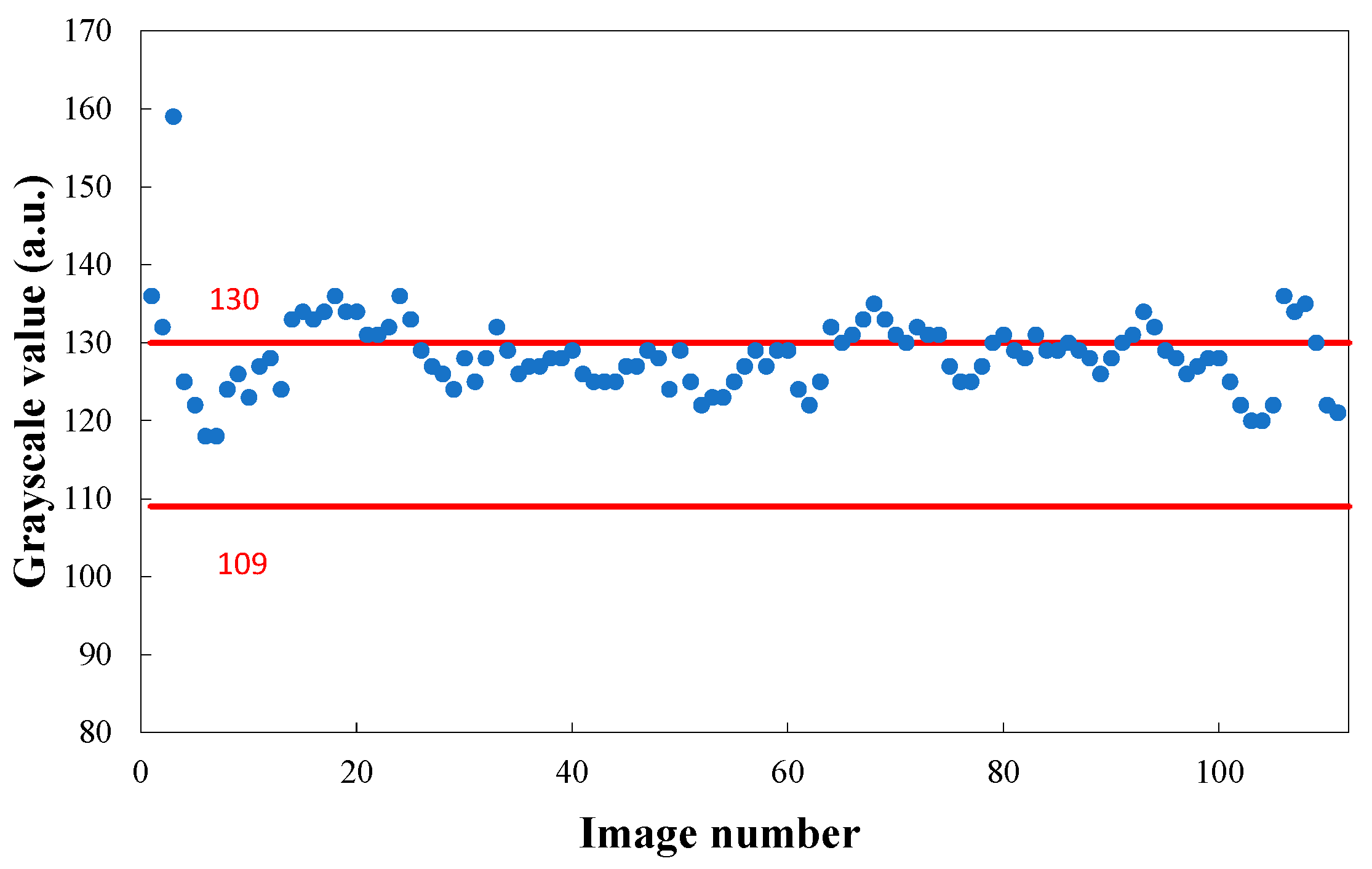
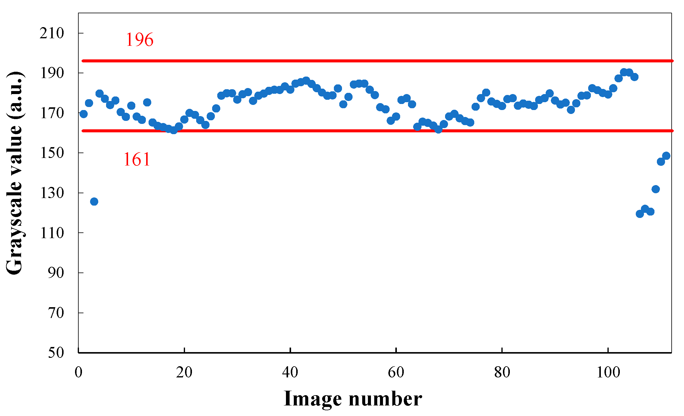
Abnormal Thermal Image Screening

This study performed a statistical analysis of data [38]. After finding the area containing the blades, the pixel position and gray-level value of the area in the grayscale image were calculated. Additionally, the full range and average value in the area were calculated. The grayscale value (μ), standard deviation σ, and other index values were used to confirm if the wind turbine blades had index values different from the normal state. We assumed that the blade was in a normal state and the full range, average value, standard deviation, and other index values of the grayscale value in the blade’s region from different viewing angles follow a normal distribution, allowing for the calculation of the 95% CI of each index value. Using this as a benchmark, when each index value was outside the CI, the variability of the index value in the image from that angle was large and abnormal. An image from this angle may capture defects. If we assume the index value is within the CI, we can select a perspective image with an index value closer to the upper and lower bounds of the interval to observe whether defects are visible in the image from that angle. This method allows “abnormal thermal images” that may contain defects to be filtered out based on the CI of each statistical index value.

Heat Accumulation Percentage Analysis for Defect Measurement

To more precisely represent the heat distribution, the grayscale value range of the blade area was divided into ten intervals. The pixel positions of the grayscale values in each interval were determined. Subsequently, the corresponding visible-light images were replaced with a specific color, changing the pixel position. Thus, the visible-light image from a specific viewing angle was segmented and superimposed on the thermal image at different intervals, and the heat distribution on the blade was visualized through a heat accumulation percentage map. Based on the thermal conduction theory, when the conductivity coefficient at the defect is small, less thermal energy is transferred, resulting in a lower temperature and a local minimum appearing in the thermal image. When the defect is thicker, the energy transfer becomes more evident. Therefore, defects can be measured by analyzing the heat accumulation percentage map of the abnormal thermal image and assessing the presence and prominence of local minima. If a defect is detected in the thermal image at a specific viewing angle, the reconstructed 3D image can be switched to that viewing angle. The defect measurement results are shown in Figure 12. The 3D image is presented on the screen corresponding to the viewing angle in the image, enabling determination of the image-shooting range and the actual location of the defect.

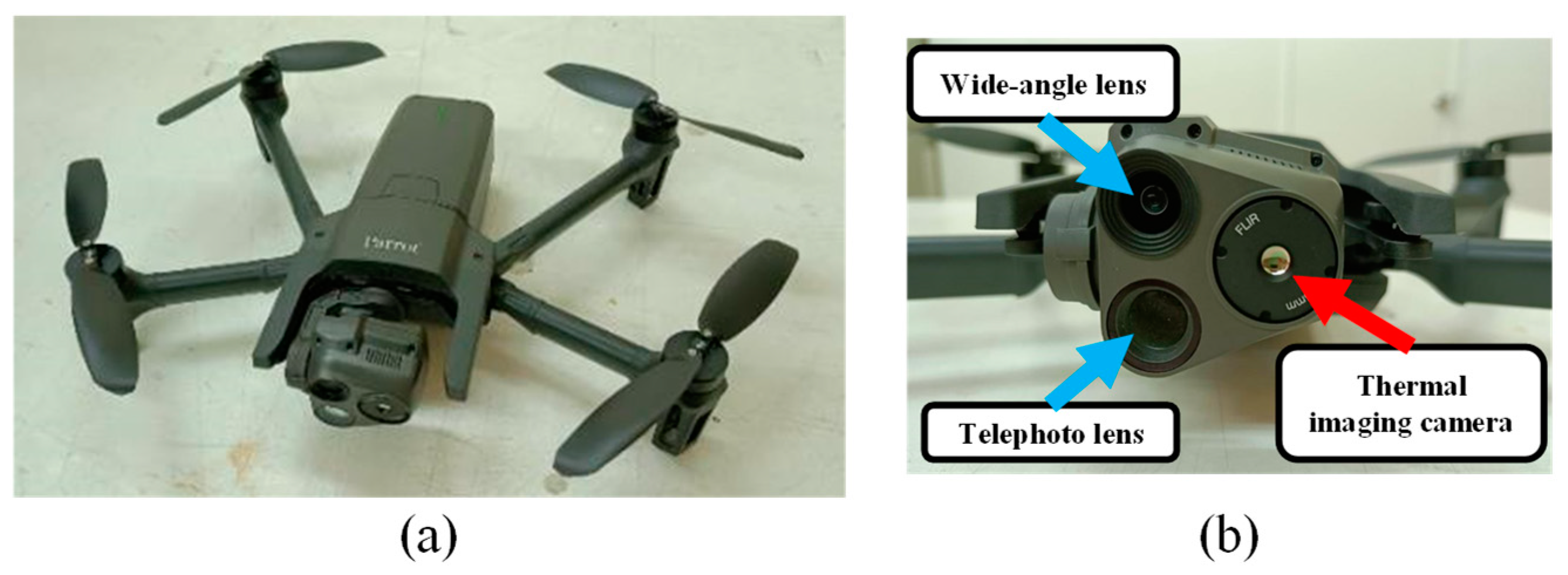
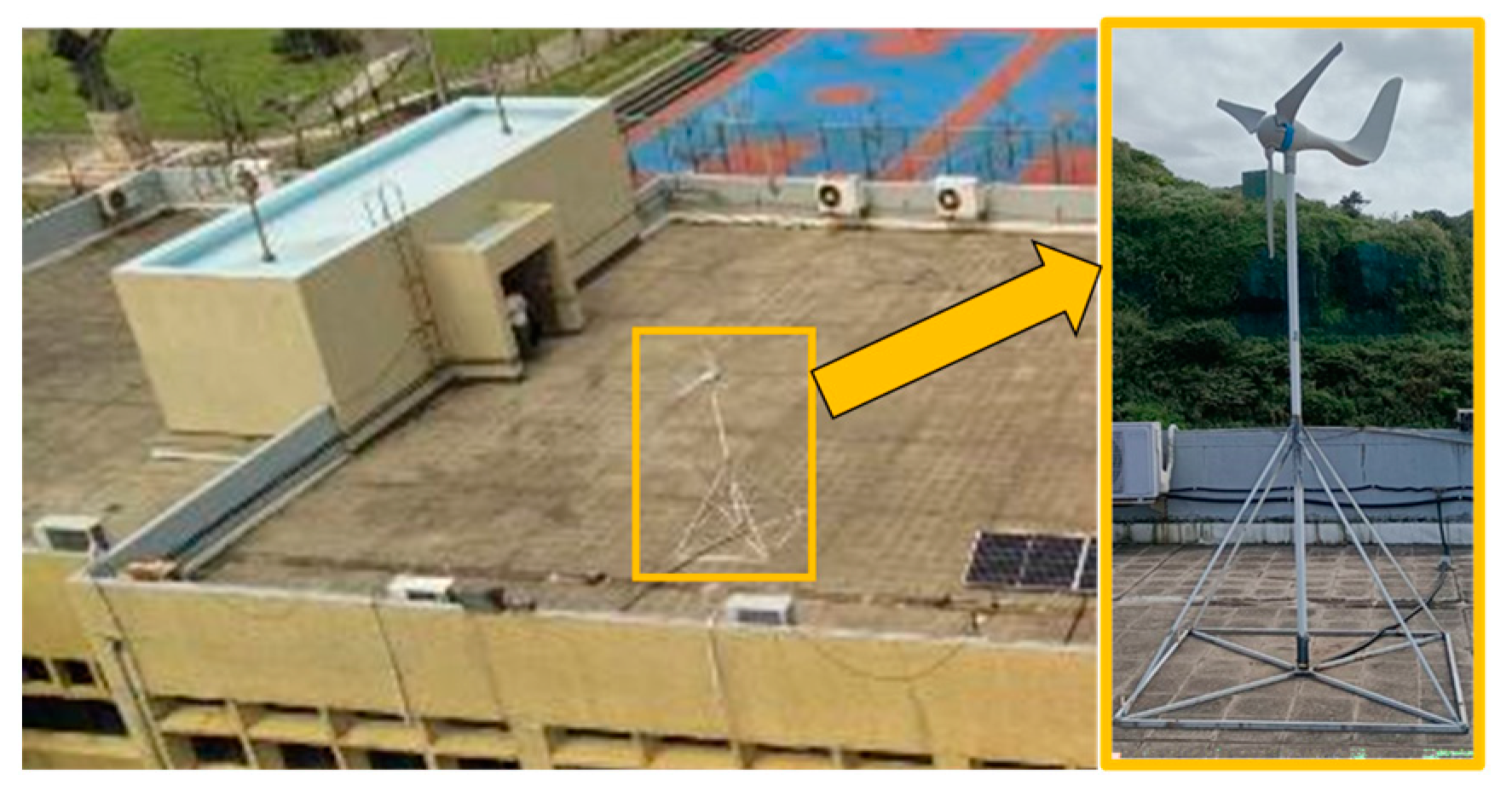
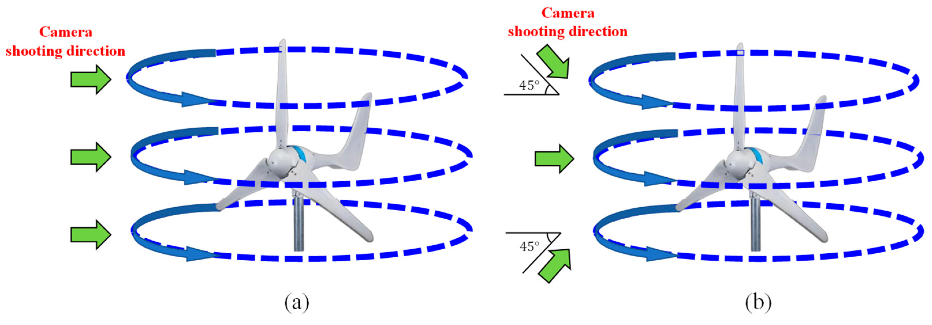
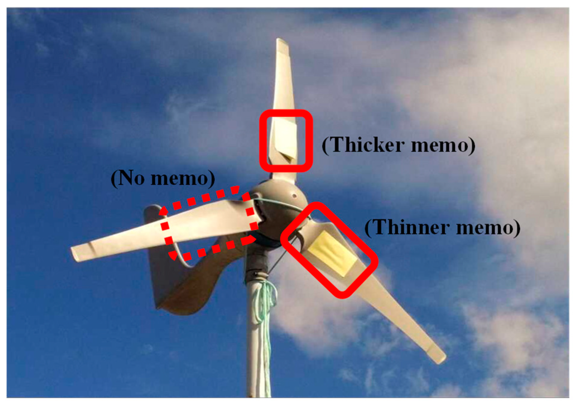
3. Measurement Experiment

This study used the Anafi-USA UAV, produced by French UAV manufacturer Parrot. Its gimbal was equipped with three lenses, as shown in Figure 13. The visible-light lens combines a wide-angle lens and a telephoto lens to achieve a 32× zoom function and 21 MP resolution. The thermal imaging camera was an FLIR Boson^® with a spectral range of 8–14 μm, a thermal resolution of 320 × 256 pixels, a temperature measurement range of −40–180 °C, and a thermal sensitivity of 0.05 °C.

This study focused on horizontally operated small wind turbines, as shown in Figure 14. Such wind turbines can be terminated by a mechanical brake, making capturing still images easier. The generator system adopted a permanent-magnet brushless generator located 2 m above the ground. The blade had a rotation radius of 1.3 m and was made of a nylon–glass fiber composite. The maximum power output was 600 W. According to the literature [39], the maximum wind speed and precipitation threshold that a common UAV can withstand to successfully take off and perform its mission are increased from 10 to 15 m/s and 0 to 1 mm/h, respectively. Therefore, this study included blade defect measurements of wind turbines based on weather temperature changes within the temperature measurement range of the thermal imaging camera and the UAV flight conditions of the reference [39].

The measurement flow chart for small wind turbines is shown in Figure 15. The Anafi-USA drone orbited the wind turbine while capturing visible-light and thermal images from different perspectives and heights. The model used the thermal image to determine the perspectives of the defect through defect measurements. It used the visible-light image for 3D reconstruction. Finally, the defect viewing angle measured by the thermal image was mapped onto the corresponding angle in the reconstructed 3D image, thereby determining the actual location of the defect.

4. Measurement Results and Discussion

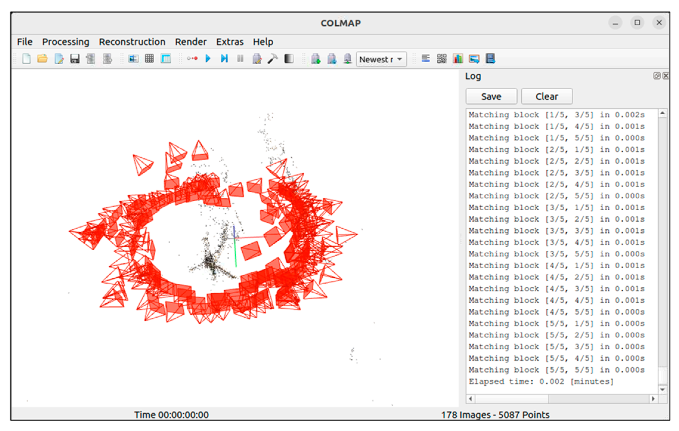
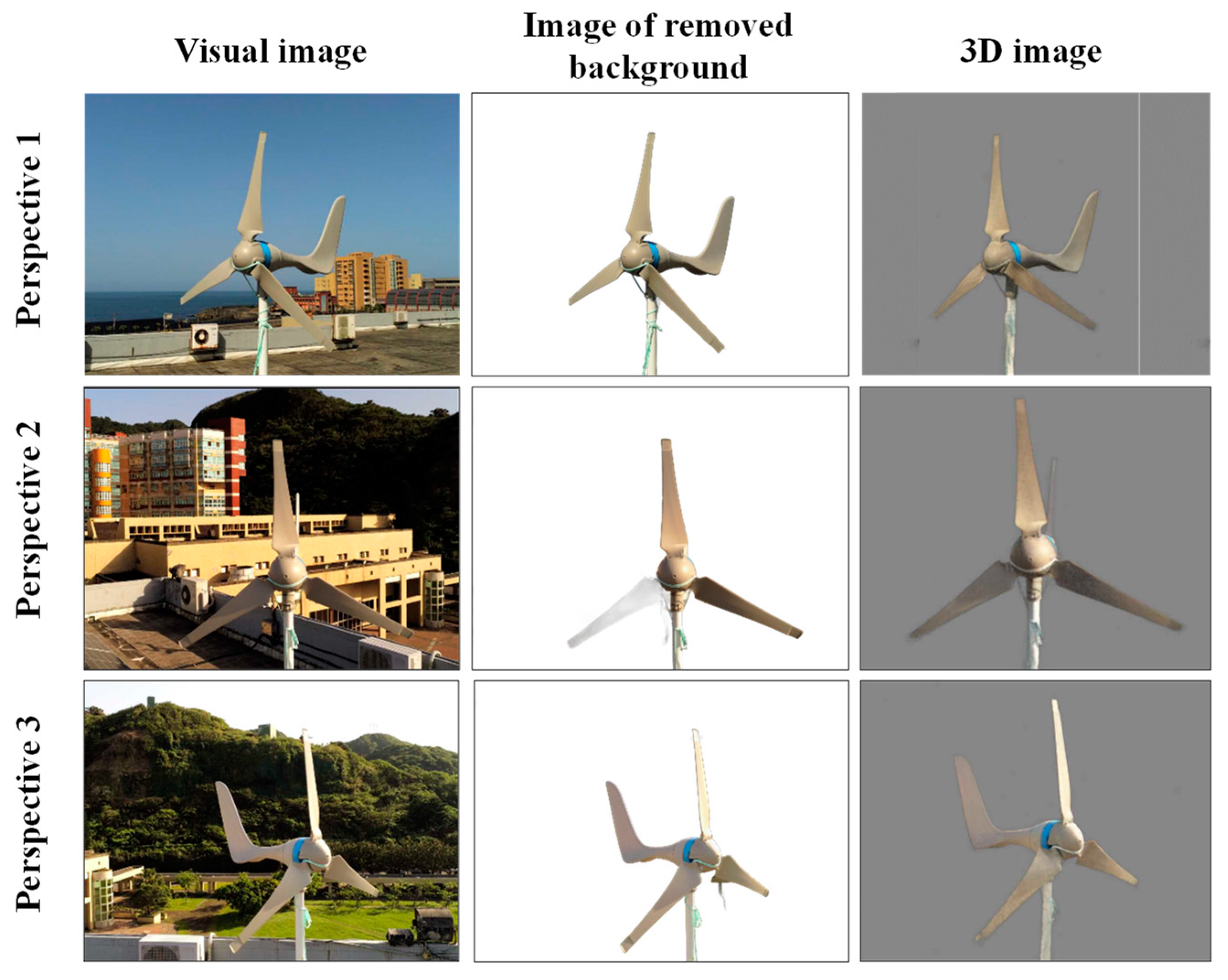
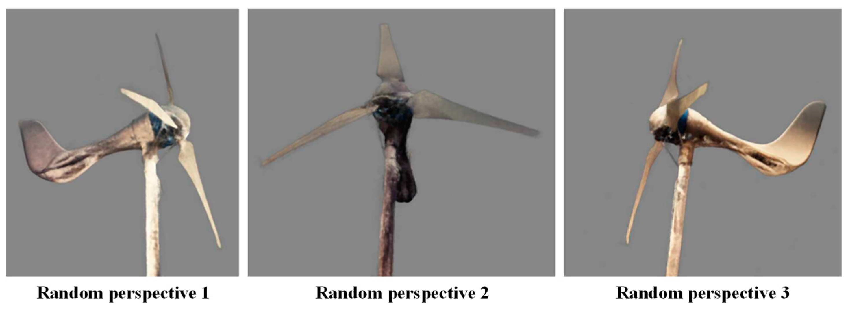
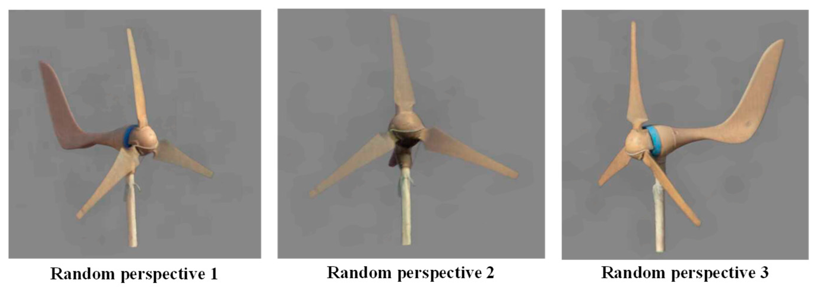
4.1. Three-Dimensional Image Reconstruction

To optimally reconstruct the 3D image of the captured scene, in addition to capturing multiple images from different perspectives, increasing the number of images shot from different angles should allow for extraction of more information from the scene. This study compared two image-shooting schemes at orthogonal and oblique angles, verifying the effect of the shooting angle on the optimization of the reconstruction results. The shooting trajectories of the two reconstruction schemes are depicted in Figure 16. To analyze the effect of 3D image reconstruction, we used the peak SNR. The PSNR is the ratio of maximum signal power to destructive noise power. It is used to verify signal reconstruction quality in image processing areas such as image compression.

In this study, the NeRF 3D reconstruction was based on the RGB color values of the input image for NN training; therefore, the PSNR value was used as an indicator to evaluate the quality of the reconstructed image. Because images have a wide dynamic range, the unit is typically expressed in logarithmic decibels (dB). According to [40], the PSNR value is crucial for judging the image reconstruction quality. The human eye cannot distinguish between original and reconstructed images if the PSNR is more than 30 dB. Therefore, a PSNR value of more than 30 dB indicates successful reconstruction.

Taking the reconstruction of a grayscale image with a single-color channel as an example, if the original image (I) and reconstructed image (K) are the same size, the maximum signal power (${max}_I$) is the maximum value of the image pixel value (255), and the destructive noise power is defined by the mean square error (MSE):

$$\mathrm{M}\mathrm{S}\mathrm{E}={\displaystyle \frac{1}{mn}}{\sum }_{i=0}^{m-1}{\sum }_{j=0}^{n-1}{\left[I\left(i, j\right)-K\left(i,j\right)\right]}^2,$$

(12)

where m and n denote the width and height of the image, respectively and $I\left(i,j\right)$ and $K\left(i,j\right)$ are the pixel values of the original and reconstructed images at positions $\left(i,j\right)$, respectively. Then, the PSNR values of the original image (I) and reconstructed image (K) can be defined as follows [40]:

$$\mathrm{P}\mathrm{S}\mathrm{N}\mathrm{R}=10\log \left({\displaystyle \frac{{{max}_I}^2}{MSE}}\right)=20\log \left({\displaystyle \frac{255}{\sqrt{MSE}}}\right),$$

(13)

The definition of the reconstruction of a color image with three color channels—R, G, and B—is similar to that of grayscale image reconstruction. The maximum signal power (${max}_I$) also uses a maximum image-pixel value of 255. In addition to the horizontal axis (m) and vertical axis (n) the destructive noise power must also consider the three color channels. The MSE values corresponding to each color treatment were summed, then divided by three to obtain the average. The PSNR values of the final original image (I) and reconstructed image (K) can be defined as follows:

$$\begin{array}{cc}\mathrm{P}\mathrm{S}\mathrm{N}\mathrm{R}& =10\log \left({\displaystyle \frac{{{max}_I}^2}{\frac{1}{3}{\sum }_{R,G,B}MSE}}\right)\hfill \\ & =10\log \left({\displaystyle \frac{{255}^2}{\frac{1}{3mn}{\sum }_{R,G,B}\left({\sum }_{i=0}^{m-1}{\sum }_{j=0}^{n-1}{\left[I_{color}\left(i,j\right)-K_{color}\left(i,j\right)\right]}^2\right)}}\right)\hfill \end{array}$$

(14)

4.1.1. Orthophoto Reconstruction Scheme

In this scheme, the drone orbited the wind turbine clockwise at three different altitudes. During this process, it maintained an upright angle without elevation or inclination, ensuring that the wind turbine remained centered in the frame (Figure 16a). A total of 208 images were captured during this period. U² Net was used to remove the backgrounds, minimizing environmental interference. The background-removed images were input into COLMAP software (3.12.0.dev0) as proposed by Schönberger et al. [23], and the results are displayed in Figure 17. Camera poses were successfully calculated for 178 out of 208 images, with a success rate of 85.6%. In addition, 5087 3D point-cloud data points were calculated. The point-cloud structure reconstructed in the interface is close to the wind turbine’s structure. After inputting the calculated camera pose and the background-removed visible-light image set into the NeRF-improved NN training of Instant NGP, the reconstructed 3D image was rendered effectively within 30 s, resulting in a PSNR value exceeding 30 dB. When the training time exceeded 30 s, the increase in the PSNR value gradually decreased until it stabilized at 35.45 dB based on a loss of 0.000285 after 5 min. The reconstructed 3D images are presented in Figure 18.

When the 3D image was switched to the initially captured viewing angles, it closely resembled the wind turbine in the visible-light image (Figure 19). The three image columns represent three of the various perspectives considered. We observe that although the background-removal effect of the left half of the blade in the background-removed image of the second perspective remains poor and semitransparent, the 3D image from this perspective remains fully visible, accurately preserving the lighting and shadows at the time of image capture. When rotated to a viewing angle different from the original capture angle, the wind turbine generator system can still be reconstructed in most cases. However, the reconstruction is limited at certain elevation angles from bottom to top due to the absence of input images from those specific angles, making the existing viewing angles insufficient to fully compensate for the missing information. Hence, the 3D image cannot be reconstructed completely or accurately. As indicated in Figure 20, black shadows and holes appear at the three arbitrary elevation angles.

4.1.2. Reconstruction Scheme of Tilt and Elevation Images

The shooting method was adjusted based on the orthophoto reconstruction scheme. The highest and lowest circular paths were shot at inclination and elevation angles of 45°, respectively (Figure 16b). A total of 230 images were captured during this period, and the U² Net algorithm was used to remove the background. The background-free image was imported into COLMAP [23], and the results are displayed in Figure 21. The camera poses were calculated for 224 out of 230 images, achieving a success rate of 97.4%. In addition, 7145 3D point-cloud data points were computed. The point-cloud structure reconstructed in the interface closely resembles the wind turbine’s structure.

After the calculated camera pose and background-removed visible-light image set were input to the NeRF trained by the improved NN of Instant NGP, the PSNR value showed that the rendering time of the 3D image reconstruction was at least 2 min. When the training time exceeded 2 min, the increase in the PSNR value gradually decreased until it stabilized after 5 min. The value reached a maximum of 32.50 dB based on a loss of 0.000681. The reconstructed 3D image is shown in Figure 22.

When the 3D image was adjusted to different viewing angles of the original image, it retained the same appearance as the wind turbine in the visible-light image. As shown in Figure 23, even when the background removal effect of the upper half of the blades in the background-removed image from the second viewing angle is poor and partially cut, the 3D image still fully reconstructs the missing portion. The appearance of the wind turbine can be restored at any rotated viewing angle. As shown in Figure 24, the complete appearance of the wind turbine can be observed from three viewing angles different from the original viewing angles.

According to the comparison of the 3D model of each viewing angle of the two schemes in Figure 20 and Figure 24, the 3D structure and texture details of the model of the tilt-angle image reconstruction scheme are clearer. We theorize that by adding images with different angles, the scheme learns additional scene information, optimizing the reconstruction and overcoming the demerits of orthophoto reconstruction schemes, in which 3D images cannot be wholly and accurately reconstructed from certain angles. Although the 3D model of the tilt-elevation image reconstruction scheme converged gradually and had a lower PSNR value, the change in the 3D image was not apparent when the PSNR value was higher than 30 dB; therefore, the impact was insignificant. Based on this discussion, future drone-based wind turbine imaging should follow the flight shooting path outlined in the tilt-elevation image reconstruction solution and incorporate images with 45° depression and 45° elevation angles.

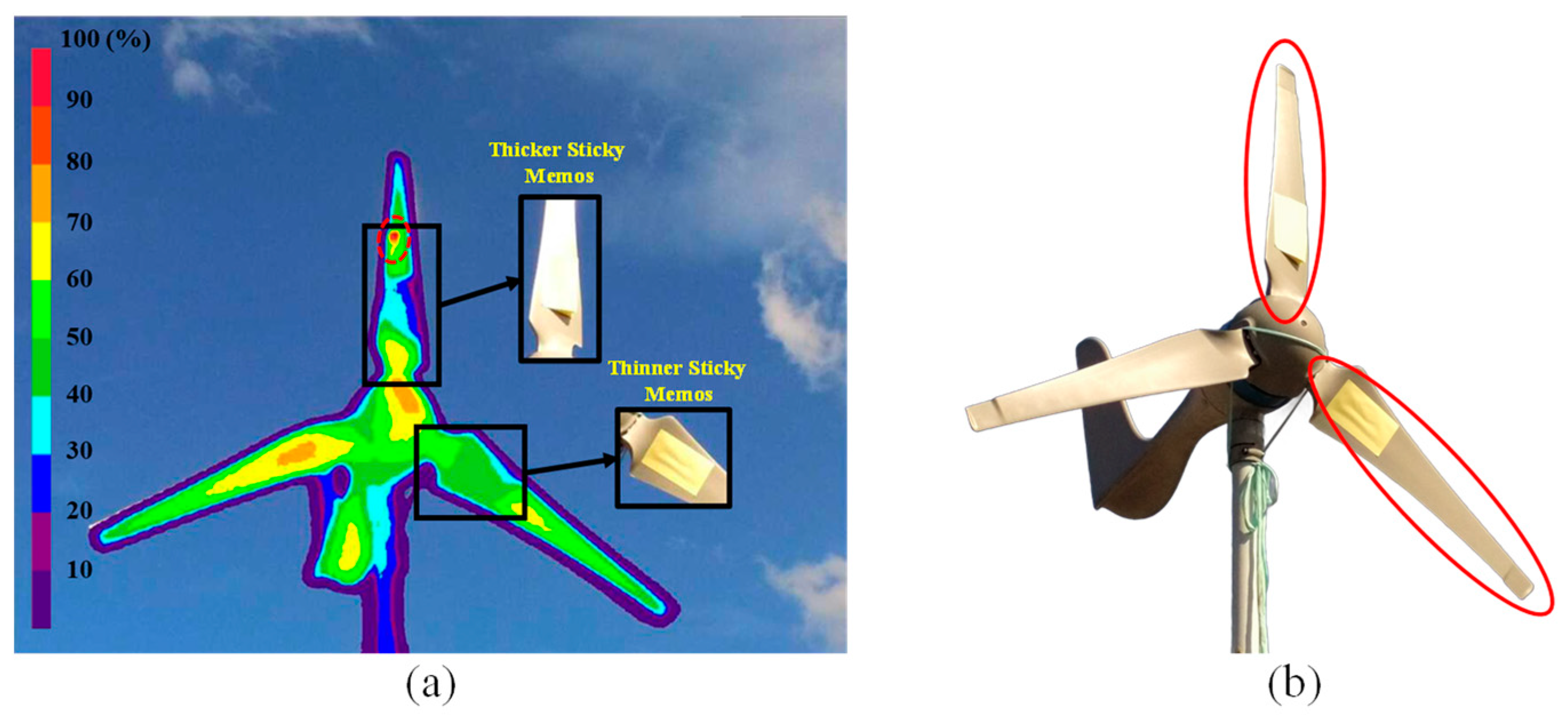
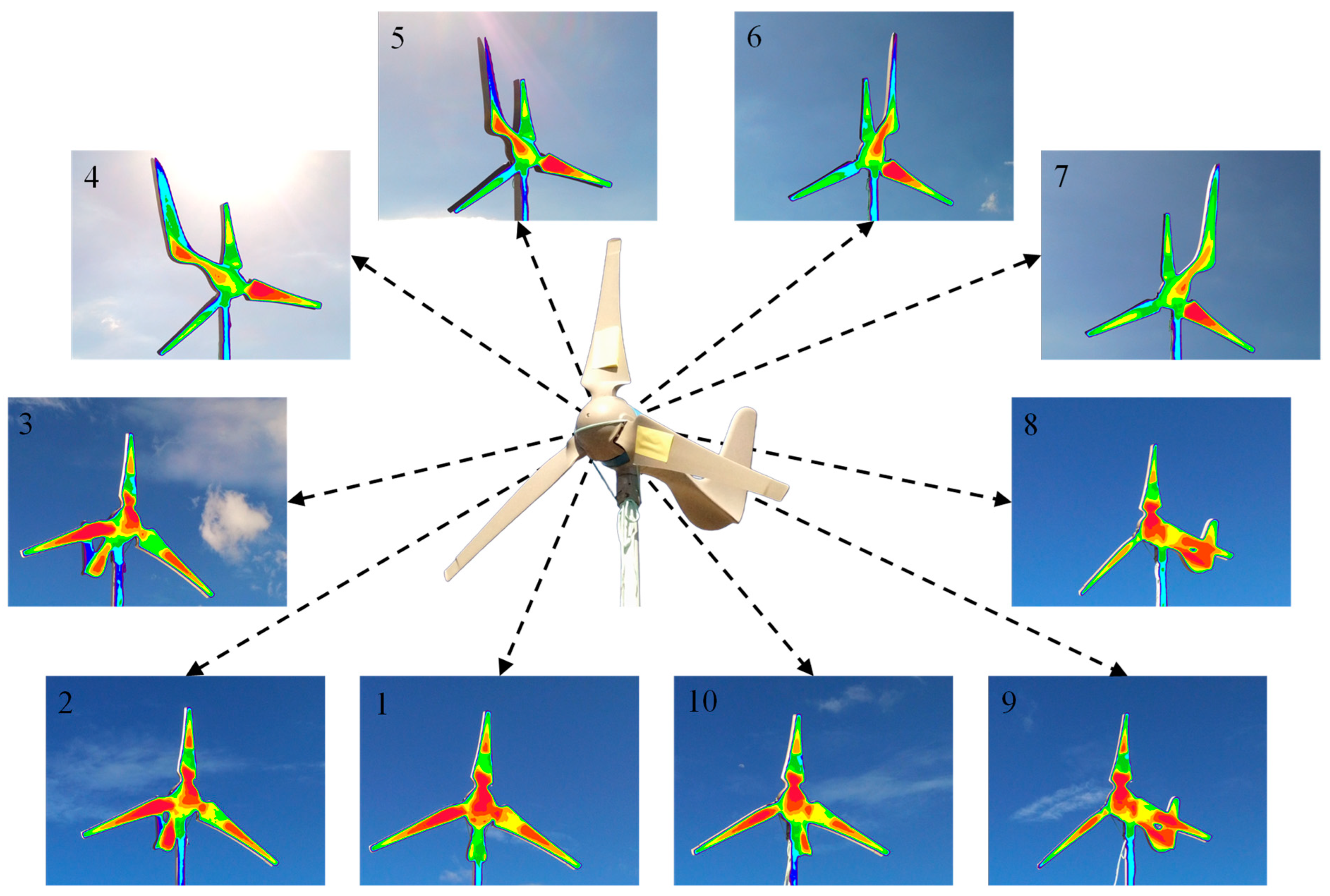
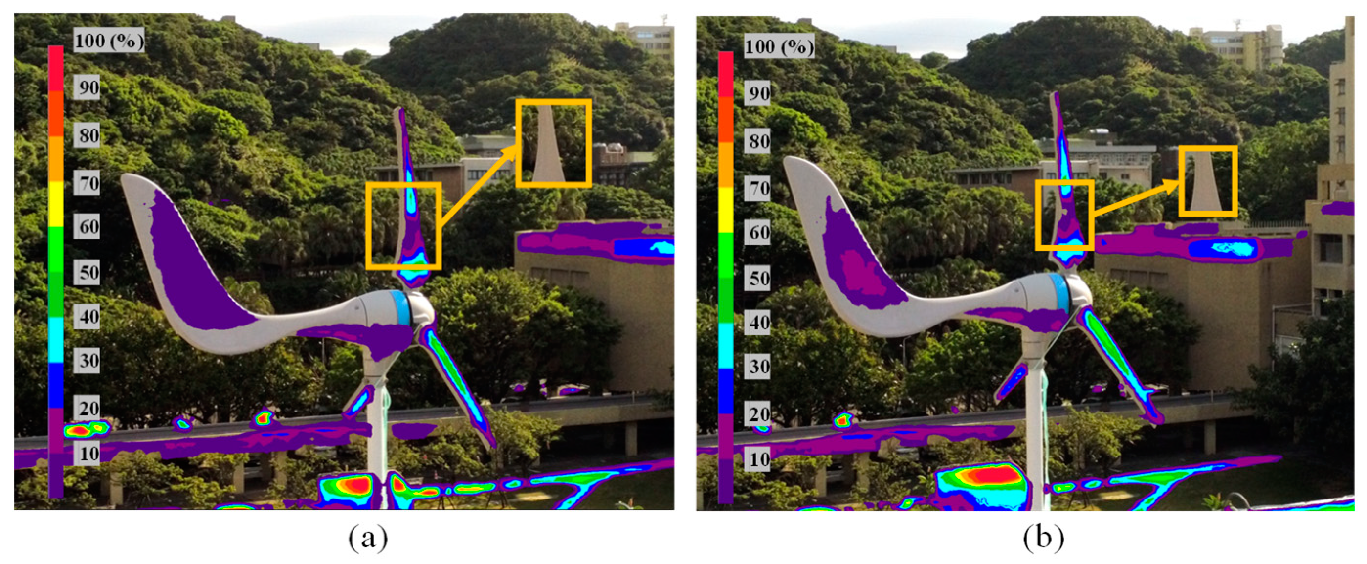
4.2. Defect Measurement

Since it is not easy to find standard experimental components for wind turbine blades with obvious deep defects, this study used sticky memos to paste on the blades to simulate the difference in surface heat conduction caused by deep defects on the blades. Figure 25 shows one of the three blades with three (thicker) sticky memos on it and another blade with one (thinner) sticky memo on it, indicating that the defects of the corresponding blade are deeper and thicker and shallower and thinner, respectively. The remaining blade, left unpasted, served as the control group for normal blades. Similarly, the tilt-angle image reconstruction scheme captured images with various viewing angles. The state of the wind turbine generator set without sticky memos was used as the “normal blade image set”, whereas the state with sticky memos was used as the “defective blade image set”.

4.2.1. Good Viewing-Angle Image Measurement

This study first analyzed the “normal blade image set” to select images with the best viewing angles. After determining the optimal threshold for each viewing-angle image using the Otsu algorithm, pixel positions with grayscale values higher than the threshold were identified, and the number of such pixels was counted to calculate the proportion of the foreground area. Based on the statistical analysis of the foreground area ratio in 92 good viewing-angle images, the average value (μ) was approximately 5.63%, and the standard deviation (σ) was approximately 11.65%. The 95% CI for the area was obtained as in [6,12].

Next, the “defective blade image set” was screened based on this trust interval. A scatter plot of the foreground area ratio for each viewing angle in the image set is presented in Figure 26. The blue dots are the foreground area ratios of the poor viewing-angle images, the red dots are the foreground area ratios of the good viewing-angle images, and the orange lines are the upper and lower bounds of the CI of the foreground area ratio. A total of 111 good viewpoint images were selected from 297 images through an initial screening within this range. Among them, 105 were classified as good viewing-angle images, while 6 were initially categorized as poor viewing-angle images but passed the screening. Nevertheless, this step removed most of the poor viewing-angle images, saving time for manual screening and judgment.

4.2.2. Abnormal Thermal Image Measurement

Similarly, the normal blade image set was analyzed. After determining the optimal threshold value of the good viewing-angle image using the Otsu algorithm, the pixel positions and grayscale values covered by the foreground area in each grayscale image were computed. The range, average value, standard deviation, and other indicators of the grayscale values were then calculated. The average value and standard deviation for each good viewing-angle image were calculated. The results are listed in

Table 1. Grayscale index values of the “normal blade image set” at various good viewing angles.

	Full Range	Average Value	Standard Deviation
Average value	119	179	30
Standard deviation	5	9	2

.

For a normal distribution of the grayscale index values of the normal blade image set, the 95% CIs of each index value are calculated as follows:

$$\left\{\begin{array}{c}\mathrm{I}\mathrm{n}\mathrm{d}\mathrm{e}\mathrm{x} \mathrm{o}\mathrm{f} \mathrm{f}\mathrm{u}\mathrm{l}\mathrm{l} \mathrm{r}\mathrm{a}\mathrm{n}\mathrm{g}\mathrm{e} \mathrm{i}\mathrm{s} \mathrm{w}\mathrm{i}\mathrm{t}\mathrm{h}\mathrm{i}\mathrm{n} \mathrm{t}\mathrm{h}\mathrm{e} 95\% \mathrm{C}\mathrm{I}\approx \left[109, 130\right]\\ \mathrm{I}\mathrm{n}\mathrm{d}\mathrm{e}\mathrm{x} \mathrm{o}\mathrm{f} \mathrm{a}\mathrm{v}\mathrm{e}\mathrm{r}\mathrm{a}\mathrm{g}\mathrm{e} \mathrm{v}\mathrm{a}\mathrm{l}\mathrm{u}\mathrm{e} \mathrm{i}\mathrm{s} \mathrm{w}\mathrm{i}\mathrm{t}\mathrm{h}\mathrm{i}\mathrm{n} \mathrm{t}\mathrm{h}\mathrm{e} 95\% \mathrm{C}\mathrm{I}\approx \left[161, 196\right]\\ \mathrm{I}\mathrm{n}\mathrm{d}\mathrm{e}\mathrm{x} \mathrm{o}\mathrm{f} \mathrm{S}\mathrm{t}\mathrm{a}\mathrm{n}\mathrm{d}\mathrm{a}\mathrm{r}\mathrm{d} \mathrm{d}\mathrm{e}\mathrm{v}\mathrm{i}\mathrm{a}\mathrm{t}\mathrm{i}\mathrm{o}\mathrm{n} \mathrm{i}\mathrm{s} \mathrm{w}\mathrm{i}\mathrm{t}\mathrm{h}\mathrm{i}\mathrm{n} \mathrm{t}\mathrm{h}\mathrm{e} 95\% \mathrm{C}\mathrm{I}\approx \left[25, 35\right] \end{array}\right.$$

Subsequently, these CIs were used to determine whether the blade was normal, allowing for the identification and elimination of the abnormal thermal images in the defective blade image set. Images were classified as abnormal if all three statistical indicator values fell outside the CIs. The scatter plots of the three statistical indicators after calculating the full range, average value, and standard deviation of all good viewing-angle images in the foreground area are illustrated in Figure 27, Figure 28 and Figure 29. The red lines in the graphs represent the upper and lower limits of the CIs for each indicator.

Among the many good viewing-angle images, only Nos. 3, 107, and 108 were regarded as abnormal thermal images, as their index values were all outside the CI. These perspective images were then observed using a thermal accumulation percentage diagram to determine the existence of local minima, which would confirm defects. In the heat accumulation percentage diagram of the image at viewing angle No. 3 (Figure 30a), unlike the continuous distribution of the normal blade in the lower-left corner, local minima can be observed in the other two blades, which correspond to the positions of the sticky memos on the blades.

Moreover, the upper blade with thicker sticky memos had a lower local minimum temperature than the blade with thinner sticky memos in the lower-right corner. It has a lower-temperature local minimum, which verifies the heat conduction theory concept according to which the thicker the defect, the more pronounced the local minimum. Therefore, according to the heat accumulation percentage diagram, the local minimum temperatures of thicker and thinner sticky memos were measured and recognized as thicker and thinner defects, respectively. In addition, 9087 mm² and 8947 mm² were calculated based on the thermal imaging spatial resolution of 1 mm/pixel and local minimum temperature, with a temperature difference of more than 10% for the areas of thicker and thinner defects, respectively. The main reason why the thicker defect is larger than the thinner defect is that the thicker sticky memos have some shadows, resulting in a larger area of local low-temperature images. The locations of the thicker and thinner defects are represented by the 3D reconstruction image shown in Figure 30b. To analyze thicker and thinner defects, this study mapped 10 thermal image viewpoints in the good viewing angle to the corresponding 3D view and measured the defect area and temperature difference effect parameters (TDEFs), as shown in Figure 31 and

Table 2. Measurement results of the thicker and thinner defect areas and TDEFs for 10 thermal image view points with corresponding 3D views at good viewing angles.

	Real Area (mm2)	1		2		3		4		5		6		7		8		9		10		Average		Standard Deviation
		Area (mm2)	TDEF (%)	Area (mm2)	TDEF (%)	Area mm2)	TDEF (%)	Area (mm2)	TDEF (%)	Area (mm2)	TDEF (%)	Area (mm2)	TDEF (%)	Area (mm2)	TDEF (%)	Area (mm2)	TDEF (%)	Area (mm2)	TDEF (%)	Area (mm2)	TDEF (%)	Area (mm2)	TDEF (%)	Area (mm2)	TDEF (%)
Thicker defect	9525	9399	27	9200	27	9087	24	9045	23	9034	21	9213	20	9346	20	9415	21	9386	28	9335	24	9246.0	23.5	150.30	3.03
Thinner detect	9525	8901	16	8944	15	8947	16	8895	19	9065	17	8840	15	8725	17	8690	16	9001	20	8890	16	8889.8	16.7	114.98	1.64

. The temperature difference effect parameter is the difference between the average heat accumulation percentage of the local minimum-temperature area and the heat accumulation percentage at its edge. According to Table 2, the area of the thicker defect in the measurement results is larger than that of the thinner defect, with average areas are 9246.0 mm² and 8889.8 mm², respectively, and standard deviations of 150.30 mm² and 114.98 mm², respectively, which are smaller than the area of the actual sticky memo (9525 mm²). The maximum error is about 7%, which can serve as practical reference value for measurement values of less than 10% error in engineering. In addition, because thicker defects are represented by thicker sticky memos, their TDEF is larger than that of thinner defects (thinner sticky memos), with mean values of 23.5% and 16.7% and standard deviations of 3.03% and 1.64%, respectively. The defect’s thickness factor affects the difference in TDEF. Since the thermal imaging sensor of the UAV used in this study only senses relative temperature changes, the actual ratio of temperature and thickness differences was not obtained. However, this study revealed that the temperature change of the defect is positively correlated with the defect thickness. In addition, the defect area and TDEF measured from the back-view angle of the wind turbine (view angles 4 to 7) are generally slightly smaller than those measured from the front-view angle (view angles 1 to 3 and 8 to 10). The reason is speculated to be that the sticky memos were all on the fronts of the blades, resulting in a weaker heat transfer effect to the back, causing the difference in measurement. Accordingly, the upper- and lower-right blades had to be removed for inspection and repair and replaced with new ones. However, the reflection of sunlight from the blades also exhibits a maximum in the heat accumulation percentage diagram, which is the area marked by the red dashed line. In addition, it had some influence on the thermal analysis.

Regarding the heat accumulation percentage graphs of image Nos. 107 and 108 (Figure 32), both images had poor viewing angles with cluttered backgrounds. These images were not selected in the previous screening of good viewing-angle images because the they had foreground area ratios of approximately 10.78% and 9.78%, respectively, without precise separation of the blades and background (barely within the 95% CI of the normal blade foreground area ratio). These two viewing angles can still be used to observe the local minimum from the blade in the heat accumulation percentage map, corresponding to the location where the sticky memo was posted. In contrast, a sticky memo cannot be observed in the visible-light image at this viewing angle, highlighting that the IR thermal effect is superior to the visible-light image. As a result, in addition to the measurement results of No. 3, the viewing angles of Nos. 107 and 108 also detected thicker sticky memos. Furthermore, based on these thermal image defect results and the reconstructed 3D image presented in Figure 30b, it was determined that they are the same thicker defect. Therefore, this study mapped the thermal image perspective of the identified defect to the corresponding view in the 3D image to confirm the actual location of the defect. Although the 3D image reconstruction technology used in this study does not obtain the actual and accurate size measurement results for defects, the results of multiple inspection angles were used to analyze whether they were the same defects, thereby reducing the misjudgment of undetected defects caused by concentrated heat from direct sunlight and ultimately improving the accuracy of defect detection. In addition, according to the simulation results reported in [41], to reduce the influences of entrance velocity and wake flow, in a wind farm, the axial distance between wind turbines needs to be 26 times the rotation diameter of the wind turbine blades and the lateral distance is required to be more than 8 times the rotation diameter of the wind turbine blades. Therefore, when a UAV performs sensing and 3D modeling at a distance of 30 m from the wind turbine, it is not difficult to measure a good viewing-angle image with the sky as the background by using the 95% CIs of each index value proposed in this study. Because the distance between wind turbines is also much greater than the measurement distance of 30 m, it is easy to miss images of other wind turbines during the measurement process. Therefore, the background image information of other wind turbines is not used and does not cause measurement errors using the method proposed in this study.

5. Conclusions

This study has presented the successful development and implementation of a UAV-assisted system for 3D reconstruction and defect detection for wind turbine blades. Utilizing visible-light images captured by drones, the system combines the U² Net method, camera pose coordinate transformation, NeRF, Instant NGP, and the marching cube algorithm to generate accurate and detailed 3D models. To enhance defect detection, thermal imaging data integrated with heat conduction sensing was employed to identify areas of local minimum temperature, which are indicative of potential defects. The system efficiently processed and reconstructed visible-light images with 3D thermal overlays, and by transforming portions of orthographic views into elevation and depression angles, the accuracy of camera pose estimation improved significantly—from 85.6% to 97.4%—resulting in clearer representations of structural and texture details. For detection of defects in wind turbines, the approach first filtered images by selecting viewpoints that represented 6% to 12% of the thermal image’s foreground area, effectively removing less informative angles. These selected images were then screened using the 95% confidence interval of statistical indicators based on normal blade conditions. Images with grayscale values outside the 109–130 a.u. range, standard deviations beyond 25–35 a.u., and mean values outside 161–196 a.u. underwent further analysis through the use of heat accumulation percentage maps. The detection of local minima within these maps confirmed the presence of defects. By mapping thermal viewpoints onto the corresponding 3D geometry, the system achieved precise spatial localization of anomalies, significantly improving both inspection accuracy and spatial interpretation. Although the 3D image reconstruction technology used in this study does not obtain actual and accurate size measurement results for defects, the results of multiple inspection angles can be used to analyze whether they capture the same defects, thereby reducing misjudgment of undetected defects caused by concentrated heat from direct sunlight and ultimately improving the accuracy of defect detection. This integrated framework overcomes the limitations of traditional single-modality inspection techniques, offering a robust, automated, and spatially accurate solution for wind turbine blade monitoring. Throughout long-term monitoring, thermal images were consistently aligned with 3D models from designated viewing angles, enabling continuous and reliable defect detection based on thermal distribution characteristics.

References

1. Kulsinskas, A.; Durdevic, P.; Ortiz-Arroyo, D. Internal Wind Turbine Blade Inspections Using UAVs: Analysis and Design Issues. Energies 2021, 14, 294. [Google Scholar] [CrossRef]
2. Memari, M.; Shakya, P.; Shekaramiz, M.; Seibi, A.C.; Masoum, M.A.S. Review on the Advancements in Wind Turbine Blade Inspection: Integrating Drone and Deep Learning Technologies for Enhanced Defect Detection. IEEE Access 2024, 12, 33236–33282. [Google Scholar] [CrossRef]
3. Rizk, P.; Rizk, F.; Karganroudi, S.S.; Ilinca, A.; Younes, R.; Khoder, J. Advanced Wind Turbine Blade Inspection with Hyperspectral Imaging and 3D Convolutional Neural Networks for Damage Detection. Energy AI 2024, 16, 100366. [Google Scholar] [CrossRef]
4. Wang, W.; Xue, Y.; He, C.; Zhao, Y. Review of the Typical Damage and Damage-Detection Methods of Large Wind Turbine Blades. Energies 2022, 15, 5672. [Google Scholar] [CrossRef]
5. Zhang, R.; Wen, C. SOD-YOLO: A Small Target Defect Detection Algorithm for Wind Turbine Blades Based on Improved YOLOv5. Adv. Theory Simul. 2022, 5, 2100631. [Google Scholar] [CrossRef]
6. Wu, Z.; Zhang, Y.; Wang, X.; Li, H.; Sun, Y.; Wang, G. Algorithm for Detecting Surface Defects in Wind Turbines Based on a Lightweight YOLO Model. Sci. Rep. 2024, 14, 24558. [Google Scholar] [CrossRef]
7. García Márquez, F.P.; Bernalte Sánchez, P.J.; Segovia Ramírez, I. Acoustic Inspection System with Unmanned Aerial Vehicles for Wind Turbines Structure Health Monitoring. Struct. Health Monit. 2022, 21, 485–500. [Google Scholar] [CrossRef]
8. Solimine, J.; Inalpolat, M. Unsupervised Acoustic Detection of Fatigue-Induced Damage Modes from Wind Turbine Blades. Wind Eng. 2023, 47, 1116–1131. [Google Scholar] [CrossRef]
9. Mielke, A.; Benzon, H.H.; McGugan, M.; Chen, X.; Madsen, H.; Branner, K.; Ritschel, T.K. Analysis of Damage Localization Based on Acoustic Emission Data from Test of Wind Turbine Blades. Measurement 2024, 231, 114661. [Google Scholar] [CrossRef]
10. Liu, Z.; Zhang, L.; Carrasco, J. Vibration Analysis for Large-Scale Wind Turbine Blade Bearing Fault Detection with an Empirical Wavelet Thresholding Method. Renew. Energy 2020, 146, 99–110. [Google Scholar] [CrossRef]
11. Loss, T.; Bergmann, A. Vibration-Based Fingerprint Algorithm for Structural Health Monitoring of Wind Turbine Blades. Applied Sciences 2021, 11, 4294. [Google Scholar] [CrossRef]
12. Panagiotopoulos, A.; Dmitri, T.; Spilios, F.D. Damage Detection on the Blade of an Operating Wind Turbine via a Single Vibration Sensor and Statistical Time Series Methods: Exploring the Performance Limits of Robust Methods. Struct. Health Monit. 2023, 22, 433–448. [Google Scholar] [CrossRef]
13. Wang, C.; Gu, Y. Research on Infrared Nondestructive Detection of Small Wind Turbine Blades. Results Eng. 2022, 15, 100570. [Google Scholar] [CrossRef]
14. Sanati, H.; Wood, D.; Sun, Q. Condition Monitoring of Wind Turbine Blades Using Active and Passive Thermography. Appl. Sci. 2018, 8, 2004. [Google Scholar] [CrossRef]
15. Collier, B.; Memari, M.; Shekaramiz, M.; Masoum, M.A.; Seibi, A. Wind Turbine Blade Fault Detection via Thermal Imaging Using Deep Learning. In Proceedings of the 2024 Intermountain Engineering, Technology and Computing (IETC), Logan, UT, USA, 13–14 May 2024; IEEE: New York, NY, USA, 2024; pp. 23–28. [Google Scholar]
16. Chen, X.; Sheiati, S.; Shihavuddin, A.S.M. AQUADA PLUS: Automated Damage Inspection of Cyclic-Loaded Large-Scale Composite Structures Using Thermal Imagery and Computer Vision. Compos. Struct. 2023, 318, 117085. [Google Scholar] [CrossRef]
17. Feroz, S.; Abu Dabous, S. UAV-Based Remote Sensing Applications for Bridge Condition Assessment. Remote Sens. 2021, 13, 1809. [Google Scholar] [CrossRef]
18. Utsav, A.; Abhishek, A.; Suraj, P.; Badhai, R.K. An IoT-Based UAV Network for Military Applications. In Proceedings of the 2021 Sixth International Conference on Wireless Communications, Signal Processing and Networking (WiSPNET), Chennai, India, 25–27 March 2021; IEEE: New York, NY, USA, 2021; pp. 122–125. [Google Scholar]
19. Morando, L.; Recchiuto, C.T.; Calla, J.; Scuteri, P.; Sgorbissa, A. Thermal and Visual Tracking of Photovoltaic Plants for Autonomous UAV Inspection. Drones 2022, 6, 347. [Google Scholar] [CrossRef]
20. Wen, B.-J.; Chen, Y.-H. Night-Time Measurement and Skeleton Recognition Using Unmanned Aerial Vehicles Equipped with LiDAR Sensors Based on Deep-Learning Algorithms. IEEE Sens. J. 2023, 23, 23474–23485. [Google Scholar] [CrossRef]
21. Chen, X.; Wang, C.; Liu, C.; Zhu, X.; Zhang, Y.; Luo, T.; Zhang, J. Autonomous Crack Detection for Mountainous Roads Using UAV Inspection System. Sensors 2024, 24, 4751. [Google Scholar] [CrossRef]
22. Zhang, K.; Pakrashi, V.; Murphy, J.; Hao, G. Inspection of Floating Offshore Wind Turbines Using Multi-Rotor Unmanned Aerial Vehicles: Literature Review and Trends. Sensors 2024, 24, 911. [Google Scholar] [CrossRef]
23. Schönberger, J.L.; Frahm, J.-M. Structure-from-Motion Revisited. In Proceedings of the IEEE Conference on Computer Vision and Pattern Recognition (CVPR), Las Vegas, NV, USA, 27–30 June 2016; pp. 4104–4113. [Google Scholar]
24. Huang, M.; Zhao, M.; Bai, Y.; Gao, R.; Deng, R.; Zhang, H. Image-Based 3D Shape Estimation of Wind Turbine from Multiple Views. In Proceedings of IncoME-VI and TEPEN 2021: Performance Engineering and Maintenance Engineering; Springer International Publishing: Cham, Switzerland, 2022; pp. 1031–1044. [Google Scholar]
25. Yang, H.; Tang, L.; Ma, H.; Deng, R.; Wang, K.; Zhang, H. WTBNeRF: Wind Turbine Blade 3D Reconstruction by Neural Radiance Fields. In Proceedings of the International Conference on the Efficiency and Performance Engineering Network, Baotou, China, 18–21 August 2022; Springer Nature Switzerland: Cham, Switzerland, 2022; pp. 675–687. [Google Scholar]
26. Tempelis, A.; Mishnaevsky, L., Jr. Erosion Modelling on Reconstructed Rough Surfaces of Wind Turbine Blades. Wind Energy 2023, 26, 1017–1026. [Google Scholar] [CrossRef]
27. Nakajima, M. Turbine Blades with Shape Estimation Using Multiple 2D Barcodes. In Proceedings of the International Workshop on Advanced Imaging Technology (IWAIT) 2023, Jeju, Republic of Korea, 9–11 January 2023; SPIE: Bellingham, WA, USA, 2023; Volume 12592, pp. 416–421. [Google Scholar]
28. Mildenhall, B.; Srinivasan, P.P.; Tancik, M.; Barron, J.T.; Ramamoorthi, R.; Ng, R. NeRF: Representing Scenes as Neural Radiance Fields for View Synthesis. Commun. ACM 2021, 65, 99–106. [Google Scholar] [CrossRef]
29. Lorensen, W.E.; Cline, H.E. Marching Cubes: A High Resolution 3D Surface Construction Algorithm. In Seminal Graphics: Pioneering Efforts that Shaped the Field; Association for Computing Machinery: New York, NY, USA, 1998; pp. 347–353. [Google Scholar]
30. Müller, T.; Evans, A.; Schied, C.; Keller, A. Instant Neural Graphics Primitives with a Multiresolution Hash Encoding. ACM Trans. Graph. 2022, 41, 1–15. [Google Scholar] [CrossRef]
31. Ruelle, D. A Mechanical Model for Fourier’s Law of Heat Conduction. Commun. Math. Phys. 2012, 311, 755–768. [Google Scholar] [CrossRef]
32. Mahmoud, M.A.; Henderson, G.R.; Epprecht, E.K.; Woodall, W.H. Estimating the Standard Deviation in Quality-Control Applications. J. Qual. Technol. 2010, 42, 348–357. [Google Scholar] [CrossRef]
33. Qin, X.; Zhang, Z.; Huang, C.; Dehghan, M.; Zaiane, O.R.; Jagersand, M. U2-Net: Going deeper with nested U-structure for salient object detection. Pattern Recognit. 2020, 106, 107404. [Google Scholar] [CrossRef]
34. Rahaman, N.; Baratin, A.; Arpit, D.; Draxler, F.; Lin, M.; Hamprecht, F.; Bengio, Y.; Courville, A. On the Spectral Bias of Neural Networks. In Proceedings of the International Conference on Machine Learning (ICML), Long Beach, CA, USA, 9–15 June 2019; PMLR: Long Beach, CA, USA, 2019; pp. 5301–5310. [Google Scholar]
35. Vaswani, A.; Shazeer, N.; Parmar, N.; Uszkoreit, J.; Jones, L.; Gomez, A.N.; Kaiser, L.; Polosukhin, I. Attention Is All You Need. In Advances in Neural Information Processing Systems (NIPS); Curran Associates, Inc.: Long Beach, CA, USA, 2017; Volume 30, pp. 5998–6008. [Google Scholar]
36. Chabra, R.; Lenssen, J.E.; Ilg, E.; Schmidt, T.; Straub, J.; Lovegrove, S.; Newcombe, R. Deep Local Shapes: Learning Local SDF Priors for Detailed 3D Reconstruction. In Computer Vision—ECCV 2020: Proceedings of the 16th European Conference on Computer Vision, Glasgow, UK, 23–28 August 2020, Part XXIX; Springer International Publishing: Cham, Switzerland, 2020; pp. 608–625. [Google Scholar]
37. Otsu, N. A threshold selection method from gray-level histograms. IEEE Trans. Syst. Man Cybern. 1979, 9, 62–66. [Google Scholar] [CrossRef]
38. Lankes, R.D.; Gross, M.; McClure, C. Cost, statistics, measures, and standards for digital reference services: A preliminary view. Ref. User Serv. Q. 2003, 43, 210–216. [Google Scholar]
39. Gao, M.; Hugenholtz, C.H.; Fox, T.A.; Kucharczyk, M.; Barchyn, T.E.; Nesbit, P.R. Weather constraints on global drone flyability. Sci. Rep. 2021, 11, 12092. [Google Scholar] [CrossRef]
40. Setiadi, D.R.I.M. PSNR vs SSIM: Imperceptibility quality assessment for image steganography. Multimed. Tools Appl. 2021, 80, 8423–8444. [Google Scholar] [CrossRef]
41. Xu, Z.; Feng, Y.H.; Zhao, C.Y.; Huo, Y.L.; Li, S.; Hu, X.J.; Zhong, Y.J. Experimental and numerical investigation on aerodynamic performance of a novel disc-shaped wind rotor for the small-scale wind turbine. Energy Convers. Manag. 2018, 175, 173–191. [Google Scholar] [CrossRef]
Figure 1. Flow chart of 3D reconstruction.
Drones 09 00342 g001
Figure 2. (a) Structure of the RSU module and (b) complete structure of the U2 Net operation process.
Drones 09 00342 g002
Figure 3. Coordinate conversion of object coordinate points when shooting images.
Drones 09 00342 g003
Figure 4. Neural radiance field (NeRF) operational process.
Drones 09 00342 g004
Figure 5. NeRF network structure.
Drones 09 00342 g005
Figure 6. Multiresolution hash coding process. (a) Calculate the hash value (f) of the grid vertex at each level; (b) retrieve the feature values in the hash table; (c) calculate the feature vector of x at each level by interpolation; (d) concatenate the feature-vector parameters of each level; (e) input the neural network.
Drones 09 00342 g006
Figure 7. Basic types of the marching cube algorithm.
Drones 09 00342 g007
Figure 8. Schematic of heat conduction distribution: (a) structure with no defects; (b) structure with defects.
Drones 09 00342 g008
Figure 9. Separation of front and rear scenes. (a) Thermal image; (b) grayscale image; (c) threshold-divided histogram; (d) area with the blade.
Drones 09 00342 g009
Figure 10. Defect measurement flow chart for wind turbines.
Drones 09 00342 g010
Figure 11. Analysis of image separation of blades and different backgrounds.
Drones 09 00342 g011
Figure 12. Defect measurement results with the 3D image switched to various viewing angles.
Drones 09 00342 g012
Figure 13. Anafi-USA UAV: (a) UAV; (b) gimbal equipped with a wide-angle lens, telephoto lens, and thermal imaging camera.
Drones 09 00342 g013
Figure 14. Small wind turbine with horizontal operation.
Drones 09 00342 g014
Figure 15. Flow chart of wind turbine defect measurement using UAV and 3D image reconstruction.
Drones 09 00342 g015
Figure 16. Schematic of UAV shooting trajectories: (a) orthophoto reconstruction scheme; (b) elevation image reconstruction scheme.
Drones 09 00342 g016
Figure 17. Camera pose calculation results of orthophoto reconstruction scheme.
Drones 09 00342 g017
Figure 18. Three-dimensional image obtained after 5 min of training of the orthophoto reconstruction method.
Drones 09 00342 g018
Figure 19. Visible-light image, background-removed image, and 3D image of the orthophoto reconstruction method from each shooting angle.
Drones 09 00342 g019
Figure 20. Incorrect perspectives of 3D image reconstruction in the orthophoto reconstruction method.
Drones 09 00342 g020
Figure 21. Camera attitude calculation results of the tilt-angle image reconstruction scheme.
Drones 09 00342 g021
Figure 22. Three-dimensional image obtained after 101.1 s of training with the tilt-angle image reconstruction scheme.
Drones 09 00342 g022
Figure 23. Visual image, image of removed background, and 3D image at each shooting angle for the tilt-angle image reconstruction method.
Drones 09 00342 g023
Figure 24. Tilt-angle image reconstruction scheme for 3D images different from the original shooting-angle images.
Drones 09 00342 g024
Figure 25. Sticky memos on the blades simulate the occurrence of defects.
Drones 09 00342 g025
Figure 26. Scatter plot of the proportion of foreground area in each viewing angle of the image set of wind turbines.
Drones 09 00342 g026
Figure 27. The 95% confidence interval (CI) of the full ranges of the defective blade image set and normal blades.
Drones 09 00342 g027
Figure 28. The 95% CI of the average value of the defective blade image set and the mean value of normal blades.
Drones 09 00342 g028
Figure 29. The 95% CI of the standard deviations of the defective blade image set and normal blades.
Drones 09 00342 g029
Figure 30. (a) Heat accumulation percentage and (b) 3D reconstruction of the image.
Drones 09 00342 g030
Figure 31. Ten thermal image viewpoints with corresponding 3D views at good viewing angles.
Drones 09 00342 g031
Figure 32. Thermal accumulation percentage of abnormal images: (a) foreground area of the image at viewing angle No. 107; (b) foreground area of the image at viewing angle No. 108.
Drones 09 00342 g032