

Impact of UAV-Derived RTK/PPK Products on Geometric Correction of VHR Satellite Imagery


Abstract
1. Introduction
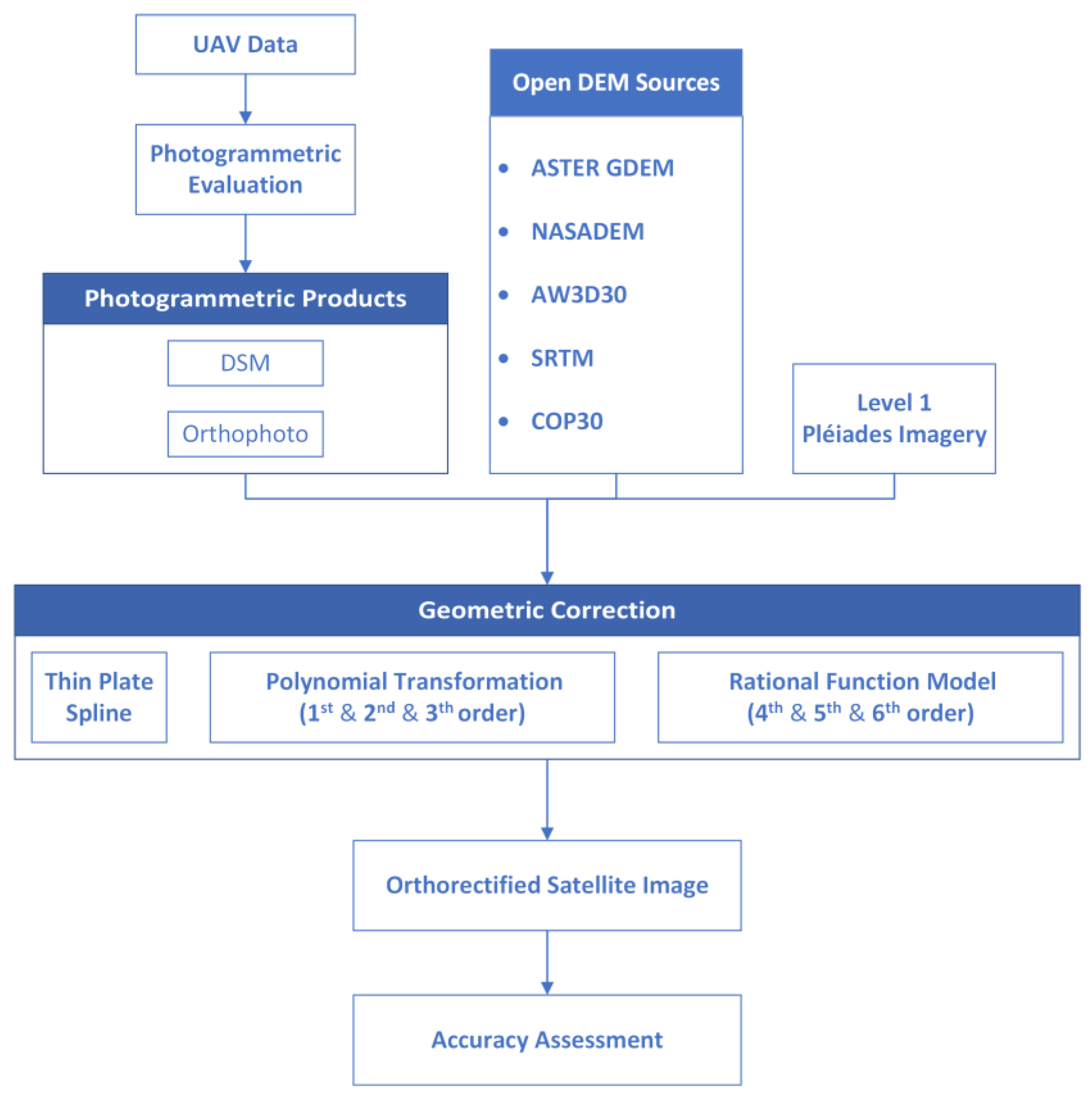
2. Methodology
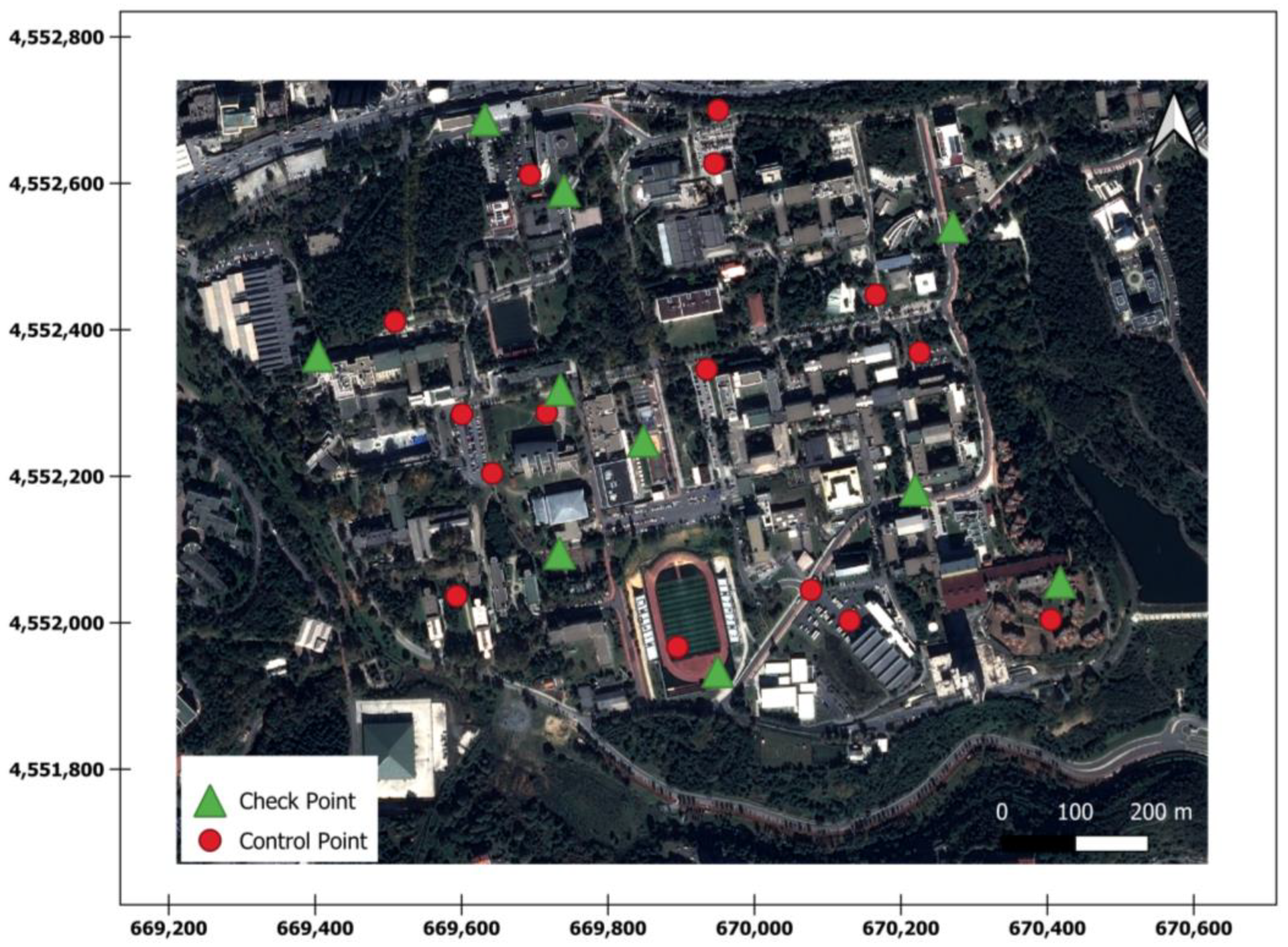
2.1. Study Area
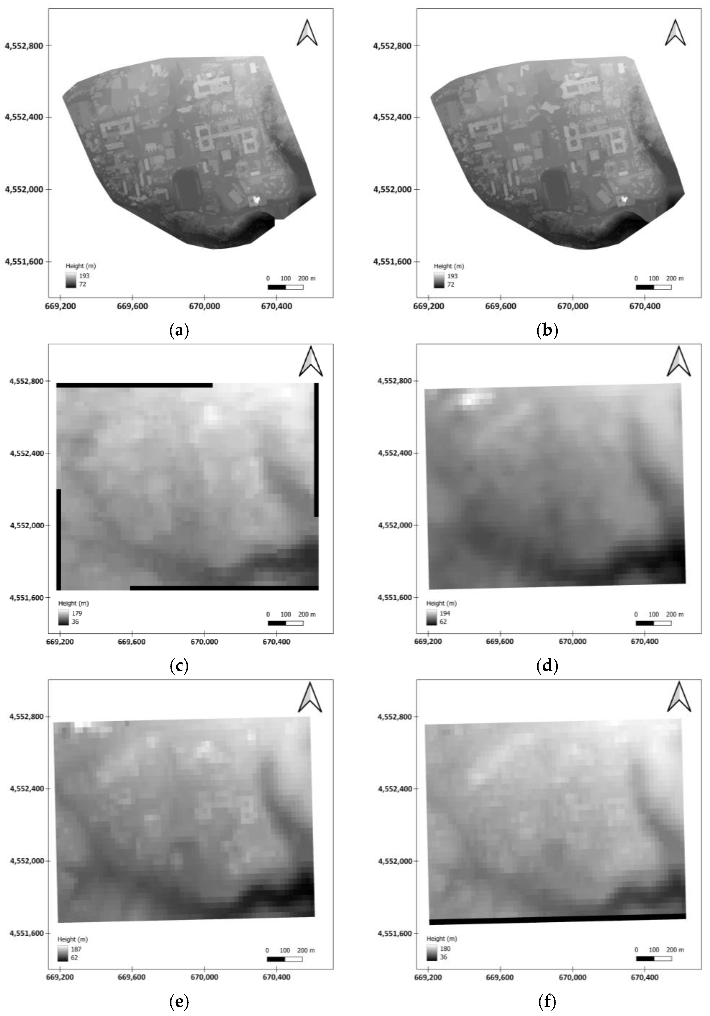
2.2. UAV-Based Photogrammetric DEM
2.2.1. Real-Time Kinematic (RTK) Positioning
2.2.2. Post-Processed Kinematic (PPK) Positioning
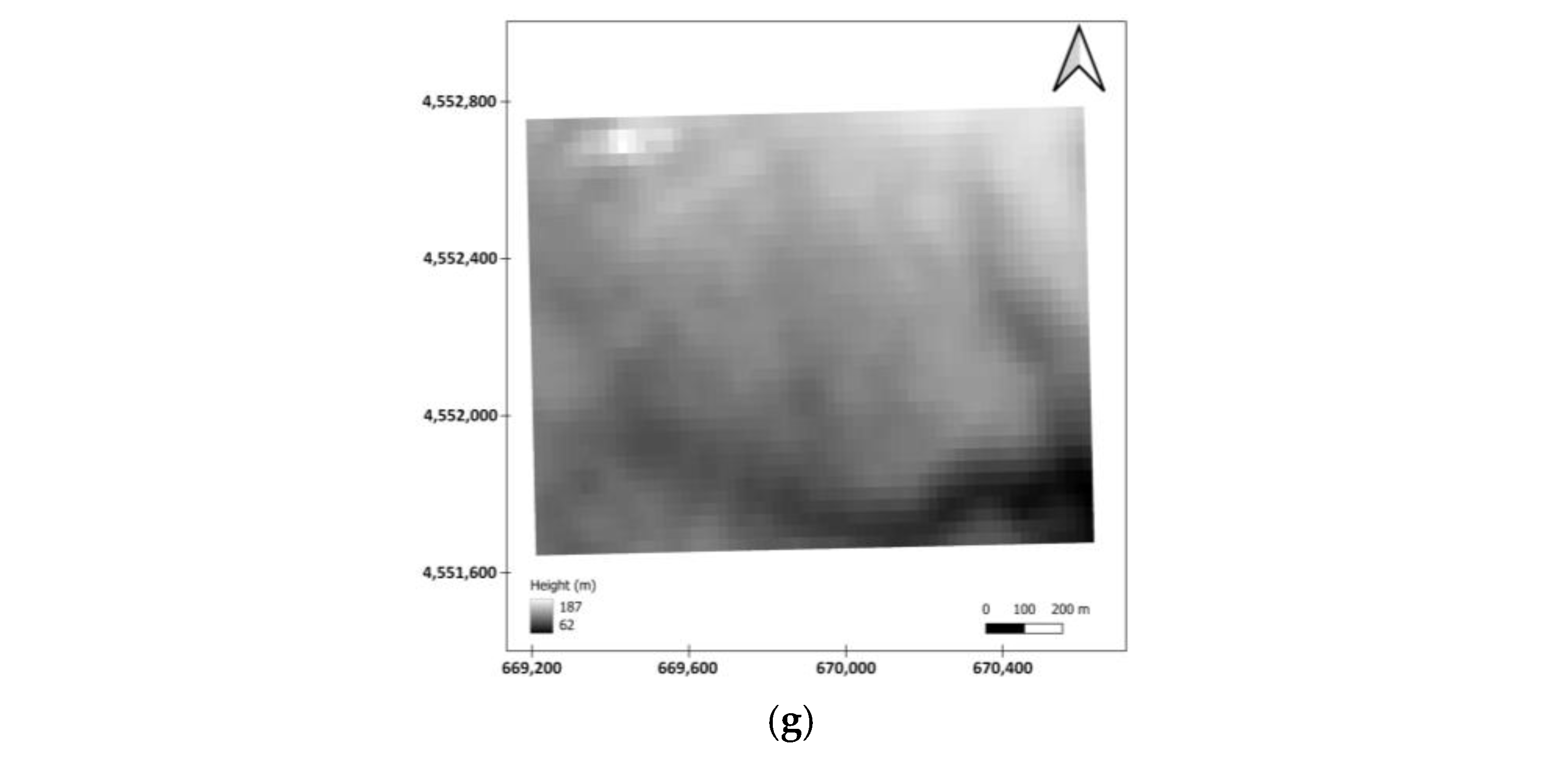
2.3. Open-Source Satellite DEM
2.3.1. Shuttle Radar Topography Mission (SRTM)
2.3.2. ASTER GDEM
2.3.3. AW3D30 DEM
2.3.4. COP30 DEM
2.3.5. NASA DEM
2.4. Geometric Correction in Remote Sensing
2.4.1. 2D Polynomial Model
2.4.2. Thin Plate Spline (TPS)
2.4.3. The Rational Function Model (RFM)
2.5. Experimental Details
3. Results

| Value | NASA DEM | Aster GDEM | AWD30 | COP30 | SRTM | RTK-DEM | PPK-DEM |
|---|---|---|---|---|---|---|---|
| Altitude | 3.181 | 3.806 | 3.007 | 2.684 | 3.388 | 0.047 | 0.039 |
3.1. Results of 2D Polynomial Model
| Method | RMSE | 1st Order | 2nd Order | 3rd Order |
|---|---|---|---|---|
| RTK | X | 0.359 | 0.643 | 0.706 |
| Y | 0.815 | 1.345 | 1.420 | |
| Total | 0.890 | 1.490 | 1.586 | |
| PPK | X | 0.347 | 0.664 | 0.692 |
| Y | 0.811 | 1.332 | 1.386 | |
| Total | 0.882 | 1.488 | 1.549 |
3.2. Results of Thin Plate Spline
| Method | Coordinate | RMSE |
|---|---|---|
| RTK | X | 0.523 |
| Y | 1.199 | |
| Total | 1.308 | |
| PPK | X | 0.515 |
| Y | 1.188 | |
| Total | 1.295 |
3.3. Results of Rational Function Model
| DEM (Spatial Resolution) | RMSE | 4th Order | 5th Order | 6th Order |
|---|---|---|---|---|
| RTK-DEM (2 cm) | X | 0.530 | 0.515 | 3.070 |
| Y | 0.397 | 0.372 | 0.345 | |
| Total | 0.662 | 0.635 | 3.089 | |
| RTK-DEM (50 cm) | X | 0.589 | 0.516 | 2.211 |
| Y | 0.340 | 0.367 | 0.437 | |
| Total | 0.680 | 0.633 | 2.254 | |
| RTK-DEM (1 m) | X | 0.591 | 0.517 | 8.276 |
| Y | 0.334 | 0.383 | 3.120 | |
| Total | 0.679 | 0.643 | 8.845 | |
| RTK-DEM (2 m) | X | 0.588 | 0.520 | 1.645 |
| Y | 0.340 | 0.392 | 0.395 | |
| Total | 0.679 | 0.651 | 1.692 | |
| PPK-DEM (2 cm) | X | 0.588 | 0.514 | 2.202 |
| Y | 0.340 | 0.379 | 0.321 | |
| Total | 0.679 | 0.639 | 2.225 | |
| PPK-DEM (50 cm) | X | 0.587 | 0.514 | 0.676 |
| Y | 0.358 | 0.337 | 0.301 | |
| Total | 0.688 | 0.615 | 0.740 | |
| PPK-DEM (1 m) | X | 0.587 | 0.513 | 1.923 |
| Y | 0.351 | 0.345 | 0.407 | |
| Total | 0.684 | 0.618 | 1.966 | |
| PPK-DEM (2 m) | X | 0.590 | 0.513 | 2.086 |
| Y | 0.338 | 0.345 | 0.304 | |
| Total | 0.680 | 0.618 | 2.108 |
| DEM | RMSE | 4th Order | 5th Order | 6th Order |
|---|---|---|---|---|
| RTK-DEM * | X | 0.530 | 0.515 | 3.070 |
| Y | 0.397 | 0.372 | 0.345 | |
| Total | 0.662 | 0.635 | 3.089 | |
| PPK-DEM * | X | 0.588 | 0.514 | 2.202 |
| Y | 0.340 | 0.379 | 0.321 | |
| Total | 0.679 | 0.639 | 2.225 | |
| ASTER | X | 0.970 | 0.552 | - |
| Y | 1.015 | 1.692 | - | |
| Total | 1.404 | 1.780 | - | |
| SRTM | X | 0.640 | - | - |
| Y | 0.614 | - | - | |
| Total | 0.887 | - | - | |
| AW3D30 | X | 0.672 | 0.592 | 2.473 |
| Y | 0.549 | 0.588 | 0.898 | |
| Total | 0.868 | 0.834 | 2.631 | |
| COP30 | X | 0.597 | 0.608 | 0.927 |
| Y | 0.739 | 0.715 | 0.865 | |
| Total | 0.950 | 0.939 | 1.268 | |
| NASADEM | X | 0.619 | 0.627 | - |
| Y | 0.709 | 0.718 | - | |
| Total | 0.941 | 0.953 | - |
4. Discussion
5. Conclusions
Author Contributions
Funding
Data Availability Statement
Acknowledgments
Conflicts of Interest
Abbreviations
| DEM | Digital elevation model |
| VHR | Very high resolution |
| UAV | Unmanned aerial vehicle |
| GNSS | Global navigation satellite system |
| PPK | Post-processed kinematic |
| RTK | Real-time kinematic |
| EO | Exterior orientation |
| GCP | Ground control point |
| RPC | Rational polynomial coefficient |
| SfM | Structure from motion |
| DSM | Digital surface model |
| DTM | Digital terrain model |
| GSD | Ground sample distance |
| CORS | Continuously operating reference station |
| SRTM | Shuttle radar topography mission |
| ASTER | Advanced Spaceborne Thermal Emission and Reflection Radiometer |
| ALOS | Advanced land observing satellite |
| NRTK | Network real-time kinematic |
| PRC | Pseudorange correction |
| CPC | Carrier phase correction |
| NASA | National Aeronautics and Space Administration |
| METI | Ministry of Economy, Trade, and Industry |
| AW3D30 | ALOS World 3D—30 m |
| ICESat | Ice, Cloud, and Land Elevation Satellite |
| GLAS | Geoscience laser altimeter system |
| PRISM | Panchromatic Remote-sensing Instrument for Stereo Mapping |
| SAR | Synthetic aperture radar |
| TPS | Thin plate spline |
| RBF | Radial basis function |
| RFM | Rational function model |
| RMSE | Root-mean-square error |
References
- Bhardwaj, A.; Sharma, S.K.; Gupta, K. Comparison of DEM Generated from UAV Images and ICESat-1datasetICESat-1 Elevation Datasets with an Assessment of the Cartographic Potential of UAV-Based Sensor Datasets. In Proceedings of the International Conference on Unmanned Aerial System in Geomatics, Roorkee, India, 2–4 April 2021; pp. 1–10. [Google Scholar]
- Carvajal-Ramírez, F.; Marques da Silva, J.R.; Agüera-Vega, F.; Martínez-Carricondo, P.; Serrano, J.; Moral, F.J. Evaluation of Fire Severity Indices Based on Pre- and Post-Fire Multispectral Imagery Sensed from UAV. Remote Sens. 2019, 11, 993. [Google Scholar] [CrossRef]
- Fiz, J.I.; Martín, P.M.; Cuesta, R.; Subías, E.; Codina, D.; Cartes, A. Examples and Results of Aerial Photogrammetry in Archeology with UAV: Geometric Documentation, High Resolution Multispectral Analysis, Models and 3D Printing. Drones 2022, 6, 59. [Google Scholar] [CrossRef]
- Biyik, M.Y.; Atik, M.E.; Duran, Z. Deep Learning-Based Vehicle Detection from Orthophoto and Spatial Accuracy Analysis. Int. J. Eng. Geosci. 2023, 8, 138–145. [Google Scholar] [CrossRef]
- Atik, Ş. Classification of Urban Vegetation Utilizing Spectral Indices and DEM with Ensemble Machine Learning Methods. Int. J. Environ. Geoinform. 2025, 12, 43–53. [Google Scholar] [CrossRef]
- Zhao, Y.; Huang, B.; Zhu, Z.; Guo, J.; Jiang, J. Building Information Extraction and Earthquake Damage Prediction in an Old Urban Area Based on UAV Oblique Photogrammetry. Nat. Hazards 2024, 120, 11665–11692. [Google Scholar] [CrossRef]
- Watson, C.S.; Kargel, J.S.; Tiruwa, B. UAV-Derived Himalayan Topography: Hazard Assessments and Comparison with Global DEM Products. Drones 2019, 3, 18. [Google Scholar] [CrossRef]
- Annis, A.; Nardi, F.; Petroselli, A.; Apollonio, C.; Arcangeletti, E.; Tauro, F.; Belli, C.; Bianconi, R.; Grimaldi, S. UAV-DEMs for Small-Scale Flood Hazard Mapping. Water 2020, 12, 1717. [Google Scholar] [CrossRef]
- Rossi, L.; Mammi, I.; Pelliccia, F. UAV-Derived Multispectral Bathymetry. Remote Sens. 2020, 12, 3897. [Google Scholar] [CrossRef]
- He, J.; Lin, J.; Ma, M.; Liao, X. Mapping Topo-Bathymetry of Transparent Tufa Lakes Using UAV-Based Photogrammetry and RGB Imagery. Geomorphology 2021, 389, 107832. [Google Scholar] [CrossRef]
- Cirillo, D.; Zappa, M.; Tangari, A.C.; Brozzetti, F.; Ietto, F. Rockfall Analysis from UAV-Based Photogrammetry and 3D Models of a Cliff Area. Drones 2024, 8, 31. [Google Scholar] [CrossRef]
- Bemis, S.P.; Micklethwaite, S.; Turner, D.; James, M.R.; Akciz, S.; Thiele, S.T.; Bangash, H.A. Ground-Based and UAV-Based Photogrammetry: A Multi-Scale, High-Resolution Mapping Tool for Structural Geology and Paleoseismology. J. Struct. Geol. 2014, 69, 163–178. [Google Scholar] [CrossRef]
- Haala, N.; Cramer, M.; Weimer, F.; Trittler, M. Performance test on uav-based photogrammetric data collection. Int. Arch. Photogramm. Remote Sens. Spat. Inf. Sci. 2012, XXXVIII-1-C22, 7–12. [Google Scholar] [CrossRef]
- Kim, H.; Hyun, C.-U.; Park, H.-D.; Cha, J. Image Mapping Accuracy Evaluation Using UAV with Standalone, Differential (RTK), and PPP GNSS Positioning Techniques in an Abandoned Mine Site. Sensors 2023, 23, 5858. [Google Scholar] [CrossRef] [PubMed]
- Martínez-Carricondo, P.; Agüera-Vega, F.; Carvajal-Ramírez, F. Accuracy Assessment of RTK/PPK UAV-Photogrammetry Projects Using Differential Corrections from Multiple GNSS Fixed Base Stations. Geocarto Int. 2023, 38, 2197507. [Google Scholar] [CrossRef]
- Tang, L.; Qiao, G.; Li, B.; Yuan, X.; Ge, H.; Popov, S. GNSS-Supported Direct Georeferencing for UAV Photogrammetry without GCP in Antarctica: A Case Study in Larsemann Hills. Mar. Geod. 2024, 47, 324–351. [Google Scholar] [CrossRef]
- Tomaštík, J.; Mokroš, M.; Surový, P.; Grznárová, A.; Merganič, J. UAV RTK/PPK Method—An Optimal Solution for Mapping Inaccessible Forested Areas? Remote Sens. 2019, 11, 721. [Google Scholar] [CrossRef]
- Famiglietti, N.A.; Cecere, G.; Grasso, C.; Memmolo, A.; Vicari, A. A Test on the Potential of a Low Cost Unmanned Aerial Vehicle RTK/PPK Solution for Precision Positioning. Sensors 2021, 21, 3882. [Google Scholar] [CrossRef]
- Stöcker, C.; Nex, F.; Koeva, M.; Gerke, M. Quality assessment of combined imu/gnss data for direct georeferencing in the context of uav-based mapping. Int. Arch. Photogramm. Remote Sens. Spat. Inf. Sci. 2017, XLII-2-W6, 355–361. [Google Scholar] [CrossRef]
- Štroner, M.; Urban, R.; Seidl, J.; Reindl, T.; Brouček, J. Photogrammetry Using UAV-Mounted GNSS RTK: Georeferencing Strategies without GCPs. Remote Sens. 2021, 13, 1336. [Google Scholar] [CrossRef]
- Eker, R.; Alkan, E.; Aydin, A. A Comparative Analysis of UAV-RTK and UAV-PPK Methods in Mapping Different Surface Types. Eur. J. For. Eng. 2021, 7, 12–25. [Google Scholar] [CrossRef]
- Cho, J.M.; Lee, B.K. GCP and PPK Utilization Plan to Deal with RTK Signal Interruption in RTK-UAV Photogrammetry. Drones 2023, 7, 265. [Google Scholar] [CrossRef]
- Ekaso, D.; Nex, F.; Kerle, N. Accuracy Assessment of Real-Time Kinematics (RTK) Measurements on Unmanned Aerial Vehicles (UAV) for Direct Geo-Referencing. Geo-Spat. Inf. Sci. 2020, 23, 165–181. [Google Scholar] [CrossRef]
- Cledat, E.; Jospin, L.V.; Cucci, D.A.; Skaloud, J. Mapping Quality Prediction for RTK/PPK-Equipped Micro-Drones Operating in Complex Natural Environment. ISPRS J. Photogramm. Remote Sens. 2020, 167, 24–38. [Google Scholar] [CrossRef]
- Bertin, S.; Stéphan, P.; Ammann, J. Assessment of RTK Quadcopter and Structure-from-Motion Photogrammetry for Fine-Scale Monitoring of Coastal Topographic Complexity. Remote Sens. 2022, 14, 1679. [Google Scholar] [CrossRef]
- Zhang, H.; Aldana-Jague, E.; Clapuyt, F.; Wilken, F.; Vanacker, V.; Van Oost, K. Evaluating the Potential of Post-Processing Kinematic (PPK) Georeferencing for UAV-Based Structure- from-Motion (SfM) Photogrammetry and Surface Change Detection. Earth Surf. Dyn. 2019, 7, 807–827. [Google Scholar] [CrossRef]
- Forlani, G.; Dall’Asta, E.; Diotri, F.; di Cella, U.M.; Roncella, R.; Santise, M. Quality Assessment of DSMs Produced from UAV Flights Georeferenced with On-Board RTK Positioning. Remote Sens. 2018, 10, 311. [Google Scholar] [CrossRef]
- Taddia, Y.; Stecchi, F.; Pellegrinelli, A. Coastal Mapping Using DJI Phantom 4 RTK in Post-Processing Kinematic Mode. Drones 2020, 4, 9. [Google Scholar] [CrossRef]
- Dinkov, D. Accuracy Assessment of High-Resolution Terrain Data Produced from UAV Images Georeferenced with on-Board PPK Positioning. J. Bulg. Geogr. Soc. 2023, 48, 43–53. [Google Scholar] [CrossRef]
- Atik, M.E.; Arkali, M. Comparative Assessment of the Effect of Positioning Techniques and Ground Control Point Distribution Models on the Accuracy of UAV-Based Photogrammetric Production. Drones 2024, 9, 15. [Google Scholar] [CrossRef]
- Famiglietti, N.A.; Miele, P.; Memmolo, A.; Falco, L.; Castagnozzi, A.; Moschillo, R.; Grasso, C.; Migliazza, R.; Selvaggi, G.; Vicari, A. New Concept of Smart UAS-GCP: A Tool for Precise Positioning in Remote-Sensing Applications. Drones 2024, 8, 123. [Google Scholar] [CrossRef]
- Cirillo, D.; Cerritelli, F.; Agostini, S.; Bello, S.; Lavecchia, G.; Brozzetti, F. Integrating Post-Processing Kinematic (PPK)–Structure-from-Motion (SfM) with Unmanned Aerial Vehicle (UAV) Photogrammetry and Digital Field Mapping for Structural Geological Analysis. ISPRS Int. J. Geo-Inf. 2022, 11, 437. [Google Scholar] [CrossRef]
- Nguyen, T. Optimal Ground Control Points for Geometric Correction Using Genetic Algorithm with Global Accuracy. Eur. J. Remote Sens. 2015, 48, 101–120. [Google Scholar] [CrossRef]
- Maras, E.E. Improved Non-Parametric Geometric Corrections For Satellite Imagery Through Covariance Constraints. J. Indian Soc. Remote Sens. 2015, 43, 19–26. [Google Scholar] [CrossRef]
- Zhang, R.; Zhou, G.; Zhang, G.; Zhou, X.; Huang, J. RPC-Based Orthorectification for Satellite Images Using FPGA. Sensors 2018, 18, 2511. [Google Scholar] [CrossRef]
- Marsetič, A.; Oštir, K.; Fras, M.K. Automatic Orthorectification of High-Resolution Optical Satellite Images Using Vector Roads. IEEE Trans. Geosci. Remote Sens. 2015, 53, 6035–6047. [Google Scholar] [CrossRef]
- Henrico, I. Geometric Accuracy Improvement of VHR Satellite Imagery During Orthorectification with the Use of Ground Control Points. Ph.D. Thesis, University of Pretoria, Pretoria, South Africa, 2016. [Google Scholar]
- Cevik, I.C.; Atik, M.E.; Duran, Z. Investigation of Optimal Ground Control Point Distribution for Geometric Correction of VHR Remote Sensing Imagery. J. Indian Soc. Remote Sens. 2024, 52, 359–369. [Google Scholar] [CrossRef]
- Ouyang, Z.; Zhou, C.; Xie, J.; Zhu, J.; Zhang, G.; Ao, M. SRTM DEM Correction Using Ensemble Machine Learning Algorithm. Remote Sens. 2023, 15, 3946. [Google Scholar] [CrossRef]
- Frey, H.; Paul, F. On the Suitability of the SRTM DEM and ASTER GDEM for the Compilation of Topographic Parameters in Glacier Inventories. Int. J. Appl. Earth Obs. Geoinf. 2012, 18, 480–490. [Google Scholar] [CrossRef]
- Gašparović, M.; Dobrinić, D.; Medak, D. Geometric accuracy improvement of WorldView-2 imagery using freely available DEM data. Photogramm. Rec. 2019, 34, 266–281. [Google Scholar] [CrossRef]
- Wang, Y.; Jiangxia, Y.; Chuan, C.; Zhou, R. Automated Geometric Precise Correction of Medium Remote Sensing Images Based on ASTER Global Digital Elevation Model. Geocarto Int. 2023, 38, 2190624. [Google Scholar] [CrossRef]
- Özcihan, B.; Özlü, L.D.; Karakap, M.İ.; Sürmeli, H.; Algancı, U.; Sertel, E. A Comprehensive Analysis of Different Geometric Correction Methods for the Pleiades -1A and Spot-6 Satellite Images. Int. J. Eng. Geosci. 2023, 8, 146–153. [Google Scholar] [CrossRef]
- Loghin, A.-M.; Otepka-Schremmer, J.; Ressl, C.; Pfeifer, N. Improvement of VHR Satellite Image Geometry with High Resolution Elevation Models. Remote Sens. 2022, 14, 2303. [Google Scholar] [CrossRef]
- Szypuła, B. Accuracy of UAV-Based DEMs without Ground Control Points. Geoinformatica 2024, 28, 1–28. [Google Scholar] [CrossRef]
- Luo, X.; Schaufler, S.; Branzanti, M.; Chen, J. Assessing the Benefits of Galileo to High-Precision GNSS Positioning—RTK, PPP and Post-Processing. Adv. Space Res. 2021, 68, 4916–4931. [Google Scholar] [CrossRef]
- Alkan, R.M.; Ozulu, I.; İlçi, V. Performance Evaluation of Single Baseline and Network RTK GNSS. MyCoordinates 2017, XIII, 11–15. [Google Scholar]
- Cina, A.; Dabove, P.; Manzino, A.M.; Piras, M.; Cina, A.; Dabove, P.; Manzino, A.M.; Piras, M. Network Real Time Kinematic (NRTK) Positioning—Description, Architectures and Performances. In Satellite Positioning—Methods, Models and Applications; IntechOpen: London, UK, 2015; ISBN 978-953-51-1738-4. [Google Scholar]
- Bolkas, D. Assessment of GCP Number and Separation Distance for Small UAS Surveys with and without GNSS-PPK Positioning. J. Surv. Eng. 2019, 145, 04019007. [Google Scholar] [CrossRef]
- EarthExplorer. Available online: https://earthexplorer.usgs.gov/ (accessed on 2 April 2025).
- Earth Science Data Systems, N. SRTM | NASA Earthdata. Available online: https://www.earthdata.nasa.gov/data/instruments/srtm (accessed on 23 February 2025).
- Earth Science Data Systems, N. New Version of the ASTER GDEM | NASA Earthdata. Available online: https://www.earthdata.nasa.gov/news/new-version-aster-gdem (accessed on 2 April 2025).
- Hayakawa, Y.S.; Oguchi, T.; Lin, Z. Comparison of New and Existing Global Digital Elevation Models: ASTER G-DEM and SRTM-3. Geophys. Res. Lett. 2008, 35. [Google Scholar] [CrossRef]
- Dataset|ALOS@EORC. Available online: https://www.eorc.jaxa.jp/ALOS/en/dataset/aw3d30/aw3d30_e.htm (accessed on 2 April 2025).
- Ecosystem, C.D.S. Copernicus DEM—Global and European Digital Elevation Model | Copernicus Data Space Ecosystem. Available online: https://dataspace.copernicus.eu/explore-data/data-collections/copernicus-contributing-missions/collections-description/COP-DEM (accessed on 4 March 2025).
- Okolie, C.J.; Mills, J.P.; Adeleke, A.K.; Smit, J.L.; Peppa, M.V.; Altunel, A.O.; Arungwa, I.D. Assessment of the Global Copernicus, NASADEM, ASTER and AW3D Digital Elevation Models in Central and Southern Africa. Geo-Spat. Inf. Sci. 2024, 27, 1362–1390. [Google Scholar] [CrossRef]
- Simard, M.; Denbina, M.; Marshak, C.; Neumann, M. A Global Evaluation of Radar-Derived Digital Elevation Models: SRTM, NASADEM, and GLO-30. J. Geophys. Res. Biogeosci. 2024, 129, e2023JG007672. [Google Scholar] [CrossRef]
- Digital Elevation/Terrain Model (DEM)|NASA Earthdata. Available online: https://www.earthdata.nasa.gov/topics/land-surface/digital-elevation-terrain-model-dem (accessed on 2 April 2025).
- NASADEM Merged DEM Global 1 Arc Second V001. Available online: https://cmr.earthdata.nasa.gov/search/concepts/C2763264762-LPCLOUD.html (accessed on 6 April 2025).
- Dönmez, Ş.Ö.; Tunc, A. Transformation methods for using combination of remotely sensed data and cadastral maps. Int. Arch. Photogramm. Remote Sens. Spat. Inf. Sci. 2016, XLI–B4, 587–589. [Google Scholar] [CrossRef]
- Schofield, W.; Breach, M. Engineering Surveying; CRC Press: Boca Raton, FL, USA, 2007. [Google Scholar]
- Keller, W.; Borkowski, A. Thin Plate Spline Interpolation. J. Geod. 2019, 93, 1251–1269. [Google Scholar] [CrossRef]
- Atik, M.E.; Ozturk, O.; Duran, Z.; Seker, D.Z. An Automatic Image Matching Algorithm Based on Thin Plate Splines. Earth Sci. Inf. 2020, 13, 869–882. [Google Scholar] [CrossRef]
- Barrodale, I.; Kuwahara, R.; Poeckert, R.; Skea, D. Side-Scan Sonar Image Processing Using Thin Plate Splines and Control Point Matching. Numer. Algorithms 1993, 5, 85–98. [Google Scholar] [CrossRef]
- Tao, C.V.; Hu, Y. Use of the Rational Function Model for Image Rectification. Can. J. Remote Sens. 2001, 27, 593–602. [Google Scholar] [CrossRef]
- Zhang, L.; He, X.; Balz, T.; Wei, X.; Liao, M. Rational Function Modeling for Spaceborne SAR Datasets. ISPRS J. Photogramm. Remote Sens. 2011, 66, 133–145. [Google Scholar] [CrossRef]
- Tao, C.V.; Hu, Y. A Comprehensive Study of the Rational Function Model for Photogrammetric Processing. Photogramm. Eng. Remote Sens. 2001, 67, 1347–1358. [Google Scholar]
- Hu, Y.; Tao, V.; Croitoru, A. Understanding the Rational Function Model: Methods and Applications. Int. Arch. Photogramm. Remote Sens. 2004, 20, 119–124. [Google Scholar]
- Schaefer, M.; Pearson, A. Chapter 19—Accuracy and Precision of GNSS in the Field. In GPS and GNSS Technology in Geosciences; Petropoulos, G.p., Srivastava, P.K., Eds.; Elsevier: Amsterdam, The Netherlands, 2021; pp. 393–414. ISBN 978-0-12-818617-6. [Google Scholar]
- Alizadeh Moghaddam, S.H.; Mokhtarzade, M.; Alizadeh Naeini, A.; Alizadeh Moghaddam, S.A. Statistical method to overcome overfitting issue in rational function models. Int. Arch. Photogramm. Remote Sens. Spat. Inf. Sci. 2017, XLII–4–W4, 23–26. [Google Scholar] [CrossRef]
Disclaimer/Publisher’s Note: The statements, opinions and data contained in all publications are solely those of the individual author(s) and contributor(s) and not of MDPI and/or the editor(s). MDPI and/or the editor(s) disclaim responsibility for any injury to people or property resulting from any ideas, methods, instructions or products referred to in the content. |
© 2025 by the authors. Licensee MDPI, Basel, Switzerland. This article is an open access article distributed under the terms and conditions of the Creative Commons Attribution (CC BY) license (https://creativecommons.org/licenses/by/4.0/).
Share and Cite
Atik, M.E.; Arkali, M.; Atik, S.O. Impact of UAV-Derived RTK/PPK Products on Geometric Correction of VHR Satellite Imagery. Drones 2025, 9, 291. https://doi.org/10.3390/drones9040291
Atik ME, Arkali M, Atik SO. Impact of UAV-Derived RTK/PPK Products on Geometric Correction of VHR Satellite Imagery. Drones. 2025; 9(4):291. https://doi.org/10.3390/drones9040291
Chicago/Turabian StyleAtik, Muhammed Enes, Mehmet Arkali, and Saziye Ozge Atik. 2025. "Impact of UAV-Derived RTK/PPK Products on Geometric Correction of VHR Satellite Imagery" Drones 9, no. 4: 291. https://doi.org/10.3390/drones9040291
APA StyleAtik, M. E., Arkali, M., & Atik, S. O. (2025). Impact of UAV-Derived RTK/PPK Products on Geometric Correction of VHR Satellite Imagery. Drones, 9(4), 291. https://doi.org/10.3390/drones9040291