Optimising Construction Site Auditing: A Novel Methodology Integrating Ground Drones and Building Information Modelling (BIM) Analysis

Abstract

Monitoring and management of construction sites are critical to ensuring project success, efficiency, and safety. Traditional methods often struggle to provide real-time, accurate, and comprehensive data, leading to delays, cost overruns, and errors. This paper presents a novel methodology utilising a ground drone for auditing construction sites to detect changes and deviations from planned Building Information Modelling (BIM). The methodology focuses on developing a novel tool that facilitates Scan-vs-BIM auditing through time. Experimental results are presented, demonstrating the effectiveness and accuracy of the proposed methodology for assessing structural discrepancies. This research contributes to advancing construction auditing practices by integrating state-of-the-art technologies and innovative techniques, ultimately enhancing project monitoring and management processes in the construction industry.

1. Introduction

Effective management of construction sites plays a crucial role in urban development, economic growth, and overall quality of life. Sustained and systematic maintenance of buildings is essential for ensuring structural safety, promoting sustainability, and improving long-term economic efficiency. As a result, the documentation and archival of construction and maintenance activities are imperative for accurately assessing structural conditions, identifying necessary repairs, and responding in a timely manner.

However, the prevalent approach for managing information related to building deterioration, maintenance history, and inspections has primarily been paper-based, manual, and inefficient [1]. Such methods pose risks of data corruption and loss during storage or handover, compromising management efficiency and accuracy. Furthermore, as construction projects become more complex and urban areas continue to expand, the volume of information that must be documented is increasing, leading to challenges such as the physical accumulation of paper records. This outdated approach to large-scale information management hinders quick decision-making and precise analysis due to difficulties in retrieving critical data when needed.

The increasing complexity of modern building construction projects has driven the need for more efficient data management systems. Traditional methods of record-keeping, such as paper logs or static spreadsheets, often fail to provide the level of organisation, accessibility, and analytical capability required for large-scale projects. As digital technologies continue to advance, construction professionals are turning to software solutions that enable better storage, tracking, and analysis of critical project data.

Automated spreadsheets with scripts or macros developed have allowed for the automation of some tasks [2]. However, despite its flexibility, spreadsheets have inherent limitations when it comes to handling complex, interconnected data structures. Furthermore, construction projects involve multiple variables, such as structural integrity assessments, material performance data, and maintenance histories, which require a more dynamic and spatially aware approach to data visualisation. In fact, one of the key drawbacks of using spreadsheets in construction management is their inability to effectively represent spatial relationships. For instance, tracking the deterioration of structural components over time, identifying wear patterns in critical areas, or linking inspection reports to specific building elements can become cumbersome in a traditional spreadsheet format.

These challenges highlight the importance of adopting more specialised digital solutions tailored to construction projects, enabling better integration of spatial and analytical data for improved decision-making and project efficiency.

The construction industry is rapidly adopting advanced digital solutions to improve project efficiency and information management. One of the most transformative innovations in this field is Building Information Modelling (BIM), a technology that revolutionises how construction data are structured, visualised, and utilised. Unlike conventional methods that depend on static 2D blueprints and written specifications, BIM creates a dynamic 3D representation of a building, integrating both its physical attributes and functional components. This allows professionals to comprehensively assess various aspects of a structure, including materials, mechanical systems, and architectural design, within a highly interactive model [3]. Beyond its role in the design and construction phases, BIM also enhances long-term facility management by consolidating essential data, such as maintenance records, structural assessments, and lifecycle predictions. The ability to centralise and visualise this information in a detailed digital model improves decision-making, reduces errors, and facilitates more effective coordination among project stakeholders. As a result, BIM is increasingly recognised as an indispensable tool for optimising both the construction and post-construction management of buildings, ensuring greater accuracy, efficiency, and sustainability throughout a structure’s lifespan.

However, the major challenge in applying the BIM methodology lies in its adaptation to real-world conditions. The models generated (as-built) often exhibit inconsistencies and become prone to errors as inevitable changes occur throughout the construction process [4,5]. The key to addressing this issue is a mechanism capable of synchronising BIM with the actual state of the project in real time, ensuring accuracy and reliability in decision-making.

2. Related Works

The Scan-vs-BIM methodology has emerged as a crucial approach in construction sites, helping to minimise discrepancies between the as-built structure and its original design within a BIM framework [6]. By comparing real-world construction data with the idealised digital model, this technique enables early detection of deviations, reducing costly errors and rework [7]. Studies have demonstrated that implementing this methodology provides significant financial benefits for engineering firms by improving accuracy and efficiency in construction quality control. To better understand the demands of the construction sector in this area, extensive research has been conducted, highlighting key challenges associated with this approach [8]. One of the primary difficulties lies in the accurate collection and processing of real-world data [9], which often contains inconsistencies such as sensor noise, misalignment, and georeferencing inaccuracies. Regarding data collection, the solution of Scan-vs-BIM involves the use of advanced geospatial technologies, including the generation of 3D point clouds from digital cameras [10] or terrestrial laser scanners (TLS) [11,12]. However, the effectiveness of the process for updating real data is often costly and sometimes inefficient (e.g., a lot of scan stations or images are required), which provides an error propagation and thus a loss of accuracy.

The need to quantify Scan-vs-BIM discrepancies has become the subject of numerous investigations [13,14,15,16]. As a result, various methods have been proposed to refine this Scan-vs-BIM methodology and enhance its reliability. Some researchers focus on improving data acquisition through image mapping, some of which includes images used for metric quality control of structural elements [17,18,19,20], while others try to improve TLS data acquisition, accurately collecting point clouds and comparing them with existing BIMs [21,22,23] during each phase of the building life cycle. In fact, the effectiveness of combining TLS and BIM has been demonstrated for preserving unconventional heritage structures, such as bridges [24,25], as well as for predicting the accuracy of the erection of pre-fabricated buildings [26], underground mining [27], building maintenance [28]. The combination of TLS and BIM provides many known advantages over other possible methodologies for the inspection of newly constructed buildings, including obtaining object data at a high level of detail with various types of information [29].

Regarding Scan-vs-BIM data processing, other authors have focused on automating basic geometries for comparison with BIM. For instance, in [30], authors developed an automated Scan-vs-BIM methodology for geometry detection and BIM updating of steel framing, significantly improving efficiency in point cloud processing and component alignment. The innovation lies in the use of genetic algorithms for instance segmentation, enabling precise axis extraction and pose transformation updates in IFC-based BIM models. However, a key limitation is that the methodology primarily updates component positioning and does not account for complex bending or twisting deformations in the BIM model, limiting its applicability to scenarios where structural elements undergo significant distortions. Other authors [31], introduced a Scan-vs-BIM methodology to automate the identification and quantification of dismantling elements in a nuclear power plant, significantly reducing errors caused by outdated drawings and human estimations. However, the approach still relies on manual verification and classification during BIM reconstruction, which may introduce human errors and inconsistencies, limiting full automation and scalability for large-scale projects.

Apart from the advances in Scan-vs-BIM data processing remarked above, one of the biggest challenges in Scan-vs-BIM is focused on passing from point clouds to BIM models in an automatic or semi-automatic way. Some recent works reported several contributions in this domain. For instance, Yunping et al. [32] introduced an automated Scan-to-BIM framework that reconstructs BIM models from defective point clouds and enables bidirectional integration between BIM and structural simulations of bridges. However, its accuracy remains sensitive to input data quality, lacking a detailed representation of complex architectural features and structural defects, which limits its applicability to intricate structures and predictive maintenance. For its part, Mun et al. [33] developed an image-based Scan-to-BIM approach that integrates photogrammetry, instance segmentation, and camera projection to enhance interior building component reconstruction with centimetre-level accuracy using widely available devices. However, its reliance on image-based point clouds makes it sensitive to occlusions, reflections, and missing data, while its assumptions of planarity and rectangularity limit its applicability to irregular or highly complex indoor environments. Trying to deal with complex geometries and structures, Garcia-Gago et al. [34] dealt with the Historical Building Information Modelling (HBIM) framework designed to enhance the diagnosis and conservation of historical buildings, effectively addressing the challenge of complex geometries in heritage structures. By integrating geometric and radiometric data from point clouds, material analysis, and non-destructive testing, the methodology enables a highly detailed and structured BIM environment capable of representing intricate architectural elements and structural deformations.

Building on the advancements described in the state of the art, this research establishes a concrete Scan-vs-BIM methodology that introduces key improvements across two fundamental areas: (i) in situ data acquisition and (ii) data processing. While previous approaches have relied on manual or semi-automated scan data processing, this study aims to enhance both automation and accuracy by integrating cutting-edge technologies through the workflow. A central innovation of this methodology is the use of a ground drone equipped with a TLS to optimise data acquisition. Unlike conventional static scanning methods, which can be limited in complex construction environments, this approach enables systematic, high-precision capture of building conditions. By improving accessibility and scan coverage, it ensures more accurate documentation of intricate geometries.

Beyond acquisition, this study advances the data processing phase of Scan-vs-BIM workflows. It introduces automated filtering techniques for noise reduction, AI-driven semantic classification, and an automatic 3D alignment method, significantly reducing the need for manual intervention. These improvements enhance the efficiency of segmenting, analysing, and processing point cloud data, ultimately streamlining the entire evaluation process. To translate these advancements into actionable insights, the methodology integrates results directly within BIM Collaborate Pro software, enabling automated model comparisons (Scan-vs-BIM). This integration facilitates precise structural discrepancy detection, enhancing quality control, deviation analysis, and automated decision-making in construction monitoring.

3. Materials and Methods

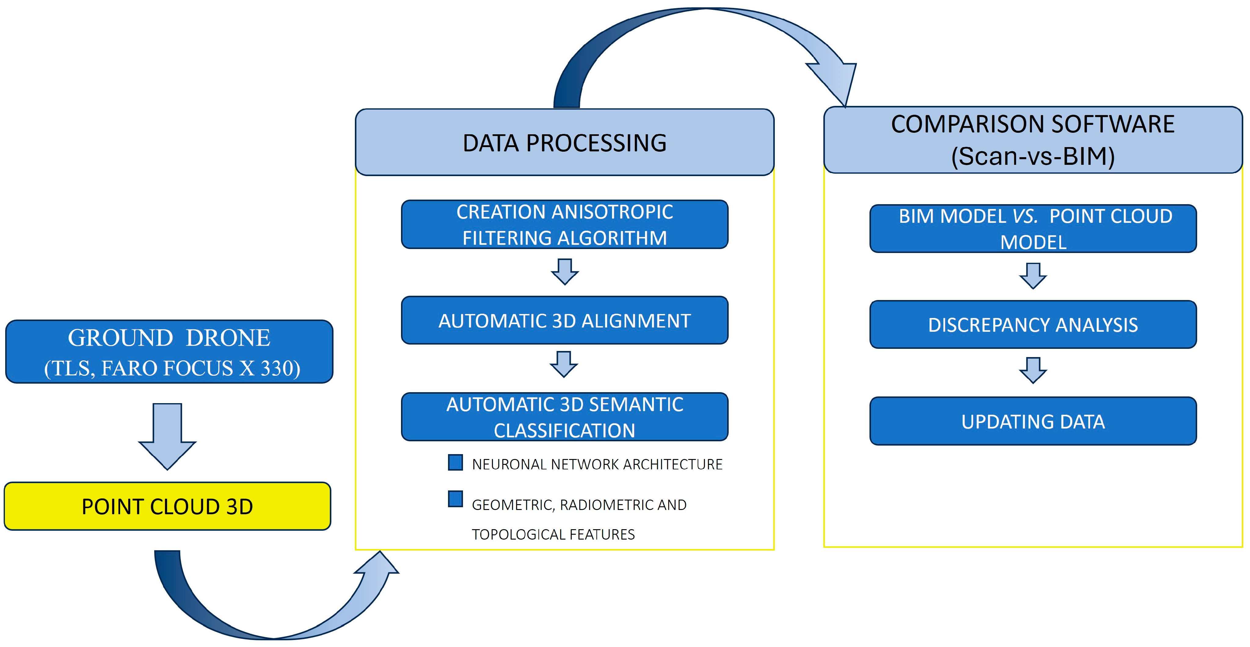
The development of a novel methodology integrating a terrestrial drone with BIM analysis is outlined in Figure 1. The first stage involves designing the terrestrial drone, along with its modular structure and interactions required to acquire the data. Once the data are collected, a second stage of data processing is carried out. In this stage, three algorithms have been developed: anisotropic filtering for noise removal, automatic 3D alignment, and semantic classification.

The processing stage generates the as-built model, commonly referred to as the point cloud model. Subsequently, the final comparison process between the as-built point cloud and the BIM (Scan-vs-BIM) is conducted using proprietary software. This software simplifies the application of the methodology and enables the detection of changes as well as the evaluation of the building works’ progress.

3.1. Ground Drone

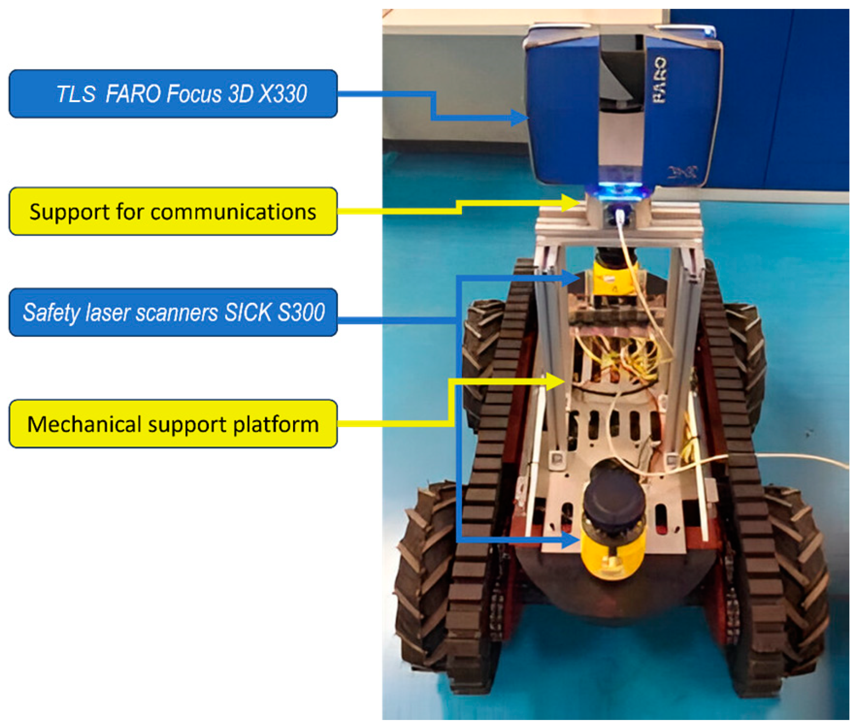
To carry out the data acquisition and the subsequent generation of the point cloud, a commercial ground drone platform (Robotnik©) is used, Figure 2, which is capable of integrating the equipment used, consisting of a control PC, that runs the software necessary for the navigation and mapping, a safety laser scanner, the TLS technology, as well as the wiring for its power supply. In addition, the ground drone features a rotation capability that facilitates navigation and improves access to capture points, which are pre-calculated by the data acquisition assistant [35]. Various mechanical and electrical modifications are made to this commercial platform to house the different elements that must be on board the ground drone, allowing the capture of points in a safe manner. Figure 2 below shows the ground drone used to carry out the research.

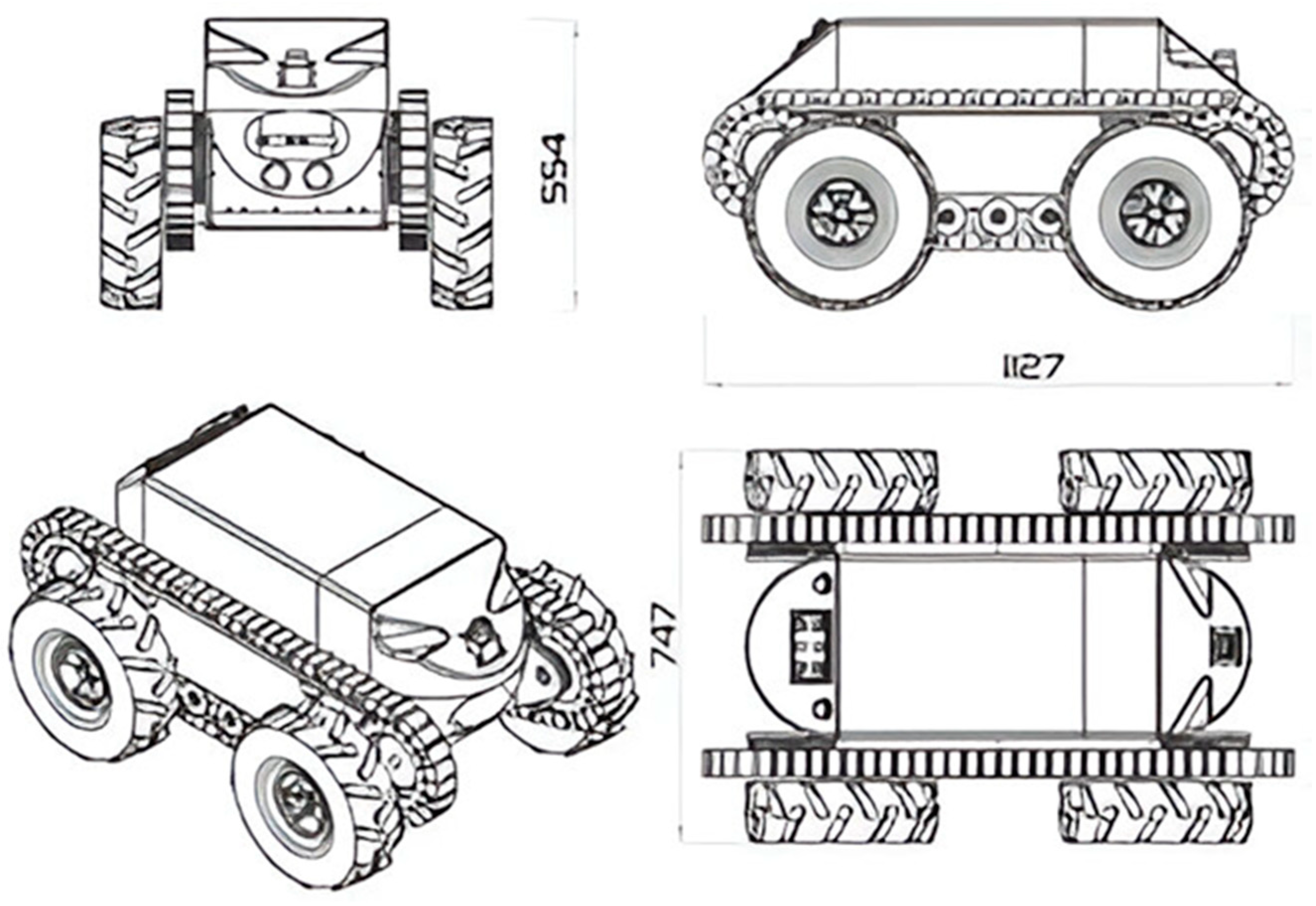
The mobile robotic platform, model Guardian, is manufactured by the company Robotnik. It is equipped with wheels and tracks for movement, providing robustness on uneven terrain. The characteristics of this platform are described in

Table 1. Ground drone platform characteristics.

Dimensions	127 × 500 × 450 mm (tracks) 1127 × 747 × 554 mm (tracks + wheels)
Weight	120 kg
Load capacity	100 kg
Maximum speed	3 m/s
Controller	Open architecture in ROS (Robot Operating System)
Autonomy	from 3 to 10 h normal operation

.

The geometric configuration of the ground drone is of particular importance to ensure accurate data collection as it directly affects the field of view of the TLS. The TLS is located at approximately 0.975 m above the ground to avoid acquiring points from the robotic platform itself, which would constitute noise in the final point cloud, and an angle of 45° concerning the vertical axis of the system is ignored during the acquisition process. In addition to the field of view, the TLS used in this research, Faro Focus 3D x330, allows the configuration of other acquisition parameters such as resolution, quality, and image acquisition. These parameters are also closely related to the acquisition time and the volume of data generated, which is of vital importance not only in mission planning but also in the development of data processing and management. A final parameter to be considered for the optimal location of the TLS stations is the measurement range of the laser scanner, which in this case varies between 0.6 m and 330 m. As the acquisition is performed inside buildings, the measurement range will be limited to 10 m, thus avoiding the capture of distant points, which may constitute noise in the final point cloud. The laser scanner technology integrated into the ground drone is designed to ensure the safety of people during the data collection stage and to accurately localise the working environment concerning the provided reference map. Additionally, two safety lasers have been implemented into the ground drone: one at the back and the other at the front in order to cover the entire construction environment. The TLS enables the capture of three-dimensional data for each area of the building, resulting in the generation of the primary point cloud. For its implementation on the ground drone platform, a mechanical support is manufactured to place the TLS 1 m above the ground vertically in the centre of the ground drone, obtaining a field of vision of 270° vertically and 360° horizontally. The assembled ground drone with all the sensors listed can be seen in Figure 3 below.

The main characteristics of the lasers and cameras selected to be part of the ground drone, which have been considered in the geometric and structural configuration of the drone, are summarised below in

Table 2. Characteristics of the primary lasers and cameras that constitute the ground drone.

FARO Focus 3D X330 Terrestrial Laser Scanner (Lake Mary, FL, USA)
Range	0.6–330 m
Measurement speed	up to 976,000 points/second
Range error	±2 mm
Integrated colour camera	up to 70 megapixels
Laser Class	Class 1
Weight	5.2 kg
Multi-Sensor	GPS, Compass, Altimeter, Dual Axis Compensator
Dimensions	240 × 200 × 100 mm
Control	via touch screen and WLAN
SICK S300 Safety Laser Scanner (Waldkirch, Germany)
Scanning range	270°
Angular resolution	0.5°
Response time	80 ms
Protective fields	up to 2 m or 3 m
Warning fields	up to 8 m
Field records	consisting of one protective field and up to two warning fields
Reset lock/parameterizable reset delay	Integrated
Switching of protective fields	Integrated
Cameras
High-resolution monochrome camera	4.92 Mpx, model IDS UI-5480CP-M-GL 1⁄2″ 2590 × 1920-14i/s-Mono-CMOS-GigE
Lower-resolution colour camera	2.12 Mpx, model IDS UI-5860CP-C-HQ 1/2.8″ Rev2 1936 × 1096-54i/s-colour CMOS-GE

.

3.2. Noise Filtering: Anisotropic Filtering

The initial stages of point cloud preprocessing involve a filtering process designed to reduce noise in the point clouds. One of the most widely used filtering methods is the Gaussian [36,37], which is based on the heat equation. However, its application has fallen into disuse due to its tendency to reduce point cloud sharpness, often leading to the loss of important details that may be critical in the context of point clouds. Trying to improve this important step in point cloud preprocessing, ref. [38] proposed a diffusion model, which they called anisotropic, based on the nonlinear variant of the heat equation, from which a filter can be constructed that minimises such loss of detail while correcting the image noise.

A particular adaptation of the anisotropic filtering method is used in this research but in a 3D domain. This anisotropic filtering technique aims to reduce the noise of 3D point clouds without losing relevant information. It is based on an iterative process of local spatial diffusion, where the points are moved considering the density of the point cloud.

3.2.1. Density Scalar Field

For the creation of an adaptative anisotropic filtering algorithm, the points in less-populated areas are adjusted to be closer to more populated areas and thus to smooth the point cloud. To do this, a scalar field of densities $\varphi$ is needed. But first, the domain of the function, $\Omega \subset {\mathbb{R}}^3$, must be defined. For this purpose, a 3D grid is created, containing the point cloud. The size of the voxel can be estimated depending on the distances of the K-neighbours (K-NN) of the point cloud. As a result, the scalar field $\varphi \left(x,y,z;t\right),$ which associates a density to each voxel of the grid, can be found by solving the anisotropic diffusion equation (Equation (1)):

$${\displaystyle \frac{\partial \varphi }{\partial t}}=\nabla ·\left[c\left(‖\nabla \varphi ‖\right)∆\varphi \right]=\nabla c·\nabla \varphi +c\left(‖\nabla \varphi ‖\right)∆\varphi$$

(1)

where $\nabla ·$, $\nabla ,$ and $∆$ are the divergence, gradient, and Laplacian operators, respectively, $c$ is the diffusion coefficient, which depends on the norm of the gradient of $\varphi$ and which controls the rate of diffusion, and the parameter $k$ controls the sensitivity to edges or sharpness. It is defined as (Equation (2)):

$$c\left(‖\nabla \varphi ‖\right)=e^{-{\left({\displaystyle \frac{‖\nabla \varphi ‖}{k}}\right)}^2}$$

(2)

For solving the previous equation, the following boundary and initial conditions are set:

• It is supposed to $\varphi \left(i,j,k;t\right)=0$ in ∂Ω.
• It is supposed to $\varphi \left(i,j,k;0\right)=\left|v_{ijk}\right|$, where $\left|v_{ijk}\right|$ represents the number of points inside the voxel $v_{ijk}$.

For approximating the spatial derivatives, the finite difference scheme is used. It is also possible to use the forward and backward differences in the boundary, instead of setting $\varphi \left(i,j,k;t\right)=0$.

As ${\displaystyle \frac{\partial \varphi }{\partial t}}\approx {\displaystyle \frac{{\varphi }^{t+1}-{\varphi }^t}{∆t}}$, the anisotropic diffusion equation can be rewritten as follows (Equation (3)):

$${\varphi }_{ijk}^{t+1}={\varphi }_{ijk}^t+∆t{\left({\nabla }_{h}c · {\nabla }_h\varphi +c{∆}_h\varphi \right)}_{ijk}^t$$

(3)

where ${\nabla }_h$ and ${∆}_h$ are the approximations of the gradient and Laplacian using finite differences. And the parameter $∆t$ is the increment of time for each iteration.

3.2.2. Point Approximation

Moving points from less-populated areas (noisy points) towards most-populated areas (non-noisy points), based on the diffusion Equation (1), it is possible to smooth the scalar field $\varphi$ and remove abrupt changes of density without losing information. This ensures that noisy points are adjusted precisely, avoiding excessively small or large steps. This translation is computed using the gradient ascent equation. Since the direction of the gradient of ϕ corresponds to the direction of a local maximum, it inherently points toward regions where data points tend to be less noisy. This is given by the following expression (Equation (4)):

$$p_{ijk}^{t+1}=p_{ijk}^t+{\gamma }_{ijk}^t{\nabla }_h{\varphi }_{ijk}^t$$

(4)

where $p_{ijk}^t$ are the points inside the voxel $v_{ijk}$ and ${\gamma }_{ijk}^t$ is the step size, which can be estimated using a Gaussian function depending on the density mean and standard deviation (Equation (5)).

$${\gamma }_{ijk}^t={\displaystyle \frac{1}{{\sigma }^t\sqrt{2\pi }}}exp\left[-{\displaystyle \frac{{\left(max\left({\varphi }_{ijk}^t,{\mu }^t\right)-{\mu }^t\right)}^2}{2{\left({\sigma }^t\right)}^2}}\right]$$

(5)

where ${\mu }^t$ is the mean and ${\sigma }^t$ the standard deviation of densities (Equations (6) and (7)):

$${\mu }^t={\displaystyle \frac{1}{\left|v_{ijk}\right|}}{\sum }_{ijk}{\varphi }_{ijk}^t$$

(6)

$${\sigma }^t=\sqrt{{\displaystyle \frac{1}{\left|v_{ijk}\right|-1}}{\sum }_{ijk}{\left({\varphi }_{ijk}^t-{\mu }^t\right)}^2}$$

(7)

Considering $max\left({\varphi }_{ijk}^t,{\mu }^t\right)$ inside the Gaussian ensures that the areas with the less density always have the maximum step size when moving its points.

In summary, for each iteration of the algorithm, the smoothed densities are computed, and the points are approximated based on these densities. In this manner, the directions in which the points move are updated with each iteration, resulting in a smoothed point cloud.

3.3. Automatic 3D Alignment

Considering that our ground drone does not use SLAM and it is based on a Stop&Go data acquisition, the point clouds acquired, although well levelled (i.e., preserve the vertical direction), need to be aligned in the same local coordinate system. To this end, the point cloud alignment is performed following a twofold process: (i) first, a ‘coarse alignment’ or first approximation is carried out based on a 3D detector and descriptor; and (ii) subsequently, a ‘fine-alignment’ of this transformation is refined by an iterative method until the minimum distance between overlapping areas is found. Both alignments make use of six-parameter rigid-solid transformations (i.e., three rotations and three translations).

In particular, the proposed automatic 3D alignment methodology employs the Harris 3D detector [39] alongside the point feature histogram (PFH) descriptor [40]. To refine the alignment, an Iterative Closest Point (ICP) algorithm is applied [41].

The Harris 3D detector yields favourable results in construction scenarios due to its suitability for identifying points on pillars, vertical walls, and ceilings by leveraging corners and edges. It operates efficiently, detecting large sets of interest points with good correspondence. The Harris 3D detector offers several variations, depending on how the trace and determinant (det) of the covariance matrix (Cov) are evaluated. In all variations, the response of the key points r(x,y,z) is computed, but distinct criteria are applied in each case. In our case, the Harris 3D Noble detector is applied (Equation (8)).

$$r\left(x,y,z\right)={\displaystyle \frac{\det \left(Cov\left(x,y,z\right)\right)}{trace\left(Cov\left(x,y,z\right)\right)}}$$

(8)

The Harris 3D detector is chosen for its focus on detecting corners and edges, while the PFH descriptor was selected for its robustness to viewpoint changes and ability to provide reliable information between point clouds. This makes it ideal for construction scenarios with varying viewpoints, lighting changes, and good scan overlap.

The 3D PFH descriptor characterises each point based on its neighbours by generalizing normal vectors (n) and mean curvature (α, ϕ, θ). These four parameters create a unique invariant signature (i.e., descriptor) for every point. For two points, p and q, a reference system of three-unit vectors (u, v, and w) is established. The difference between the normal vectors at p (n_p) and q (n_q) is then described using the normal vectors and three angular variables (Equations (9) and (11)), with d representing the distance between p and q.

$$\alpha =arc\cos (v·n_q)$$

(9)

$$\mathrm{\varnothing }=arc\cos (u·{\displaystyle \frac{p-q}{d}})$$

(10)

$$\theta =arc\tan (w·n_p,u·n_p)$$

(11)

being

$$v=u\times {\displaystyle \frac{p-q}{d}}; w=u\times v; d={\left|\left|p-q\right|\right|}_2$$

The 3D PFH descriptor is applied to all feature points identified by the Harris 3D Noble detector, associating each point with a description. These descriptions are used to find correspondences between points from different point clouds. Identifying corresponding points enables the calculation of the transformation needed to align the point clouds within the same local coordinate reference system.

After computing the Harris 3D detector and PFH descriptor and applying an initial coarse alignment to all the point clouds, some are correctly aligned while others are not. This misalignment occurs due to similarities between scans, leading to imperfections. Despite this, the point clouds are brought close to their real positions, allowing for the creation of a single unified 3D point cloud through a final alignment process that corrects these errors. The final adjustment is performed using the ICP algorithm, an iterative method that minimises the distance error between point clouds until perfect alignment is achieved. Each iteration involves three steps: (i) identifying pairs of corresponding points, (ii) calculating the transformation that minimises the distance between these points, and (iii) applying the transformation to the point clouds. Because ICP is iterative, a good initial approximation is crucial for convergence. This initial estimate is provided by the coarse alignment, which approximates the point clouds’ positions effectively.

The main advantage of the two-step Harris 3D/PFH and point-to-point ICP registration is its fully automated nature. It eliminates the need for user interaction or the placement of targets in the scene as the method relies on naturally occurring points of interest within the environment.

3.4. Semantic Classification

The process of point cloud semantic classification is essentially an automatic process of segmenting the point cloud based on geometric and radiometric features and statistical rules rather than explicit supervised learning or prior knowledge [42]. This task can be performed using machine learning [43,44] or more specifically, within the subfield of deep learning [45,46], given the volume of data extracted from common point clouds. Current research on point cloud segmentation using deep learning methodologies focuses on weakly supervised semantic segmentation, domain adaptation in semantic segmentation, semantic segmentation based on multimodal data fusion, and real-time semantic segmentation [47].

The methodology employed in the semantic classification of the point clouds obtained in this research is focused on the use of deep learning and especially in the combination of geometric, radiometric, and topological features. The process, which has yielded satisfactory results in comparing the classification of point cloud structures with their equivalent BIMs, is detailed below.

3.4.1. Neural Network Architecture

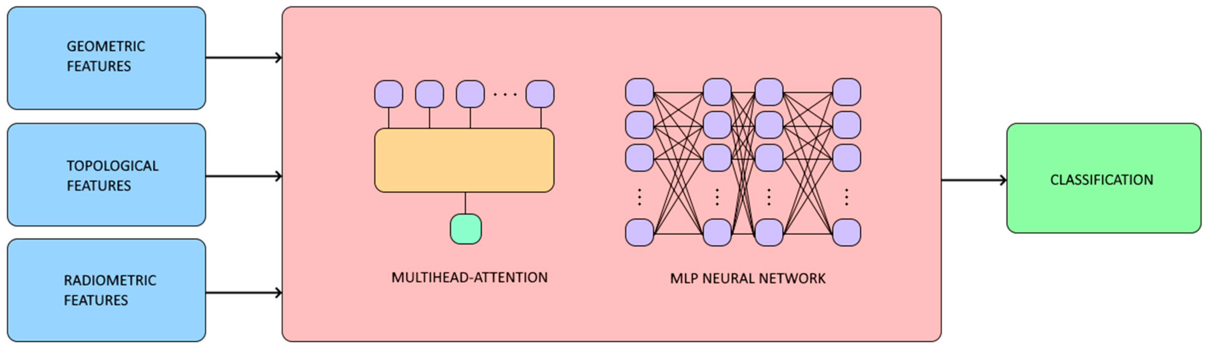
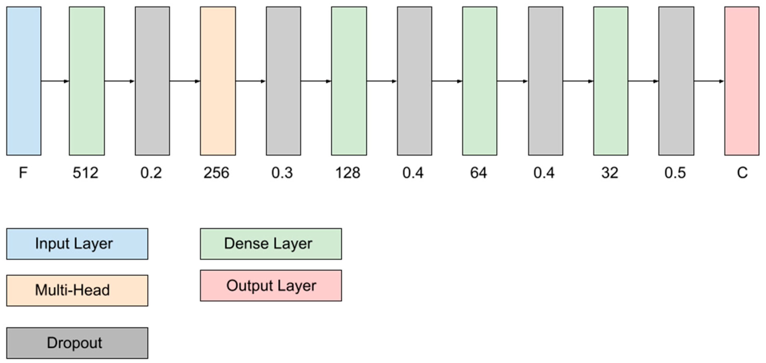
The proposed neural network architecture for 3D point cloud classification is designed to take advantage of the radiometric, geometric, and topological features of each point (Figure 4). These features constitute the input to the model and play a crucial role in capturing the underlying structure and context within the point cloud. In the following, the architecture is detailed, with special emphasis on the multi-head attention mechanism, which is fundamental for modelling the complex interactions between the points.

The model input consists of feature vectors associated with each point in the cloud. Each vector includes radiometric (colour, intensity, and/or reflectance), geometric (geometric features extracted from the covariance matrix), and topological (distance to the plane, height above, and height below) information. These multidimensional features are essential to fully describe the nature of the point and its neighbourhood.

At the core of the architecture, there is a multi-head attention layer (Figure 4), which allows the model to learn both local and global relationships between points in the cloud. This mechanism operates by assigning adaptive weights to interactions between points, allowing the network to identify relevant patterns and key relationships in the data. This layer is implemented by dividing the internal feature representations into multiple subspaces (i.e., attention heads), each focusing on different aspects of the interactions. This ensures that the model captures a diversity of spatial and contextual relationships. By combining the outputs of all heads, the model achieves a rich and robust representation of the dependencies between points.

After multi-head attention, a layer normalisation is applied to stabilise the training and improve the convergence of the model. The processed features are flattened to connect them to the subsequent dense layers.

The final part of the model consists of several fully connected dense layers. These layers are designed to perform classification based on the processed features. To mitigate overfitting, regularisation techniques such as L2 penalty and dropout are employed, which improve the generalisation of the model.

All the outputs of each layer are evaluated in the rectified linear unit (ReLU) function (Equation (12)):

$$ReLU \left(z\right)=R\left(z\right)=\mathrm{m}\mathrm{a}\mathrm{x}(0,z)$$

(12)

In simple terms, the softmax function applies the exponential function to each element z_i of the input vector z. It then normalises these values by dividing each exponential by the sum of all exponentials in the vector. This normalisation ensures that the components of the output vector ${\sigma \left(z\right)}_i$ sum to 1.

In point cloud classification problems, the Categorical Cross Entropy loss function is commonly used due to its effectiveness in measuring the difference between the actual class distribution and the model’s predictions. It is rooted in the concepts of entropy and probability, making it well suited for this type of task. Then, the Categorical Cross Entropy function is defined as Equation (13):

$$L=-{\sum }_i{y}_i\mathrm{l}\mathrm{o}\mathrm{g}\left({\widehat{y}}_{i }\right)$$

(13)

where $y_i$ represents the actual class label, and ${\widehat{y}}_{i }$ denotes the prediction (probability between 0 and 1).

The training consists of two phases, forward propagation and back propagation. Forward propagation is based on everything defined above, i.e., the output z is calculated, evaluated in the activation function, and, finally, with the output of the last layer, the loss function L is calculated. Back propagation is the weight adjustment process that minimises the loss function. It is applied after forward propagation. For this purpose, the following Gradient Descent method is used:

• The gradient of L concerning the weights w and biases b is calculated (Equation (14)).

$$\nabla L=\left({\displaystyle \frac{\partial L}{\partial w}},{\displaystyle \frac{\partial L}{\partial b}}\right)=-\left({\displaystyle \frac{\partial }{\partial w}}{\sum }_i{y}_i\log \left({\widehat{y}}_{i }\right),{\displaystyle \frac{\partial }{\partial b}}{\sum }_i{y}_i\log \left({\widehat{y}}_{i }\right)\right)$$

(14)

• The weights and biases are updated using the negative gradient multiplied by the learning rate γ (Equations (15) and (16)):

$$w_{t+1}=w_t-\gamma {\displaystyle \frac{\partial L}{\partial w}}$$

(15)

$$b_{t+1}=b_t-\gamma {\displaystyle \frac{\partial L}{\partial b}}$$

(16)

The process of forward propagation and back propagation is repeated several times (epochs) until the loss function L is minimised. After completing the training process, the neural network’s neurons and weights are adjusted to minimise the output error (i.e., the loss function is minimised). Once trained, it is sufficient to input the geometric, radiometric, and topological features of the points to be classified into the input layer and perform forward propagation again. The classification is then determined based on the predictions generated by the output layer.

3.4.2. Geometric and Topological Features

The geometric features of a point are given by the eigenvalues and eigenvectors of the covariance matrix ${\mathsf{\Sigma }}_N$ of its neighbourhood $N \left(\mathrm{E}\mathrm{q}\mathrm{u}\mathrm{a}\mathrm{t}\mathrm{i}\mathrm{o}\mathrm{n}\right(17\left)\right)$:

$${\mathsf{\Sigma }}_N=\left(\begin{array}{ccc}{S}_{xx}& S_{xy}& S_{xz}\\ S_{yx}& S_{yy}& S_{yz}\\ S_{zx}& S_{zy}& S_{zz}\end{array}\right) S_{xy}={\displaystyle \frac{1}{n-1}}{\sum }_{i=1}^n(x_i-\overline{x})(y_i-\overline{y})\hspace{1em}\overline{x}={\displaystyle \frac{1}{n}}{\sum }_{i=1}^n{x}_i$$

(17)

where $x=\left\{x_1,x_2,\dots ,x_n\right\},y=\left\{y_1,y_2,\dots ,y_n\right\},z=\left\{z_1,z_2,\dots ,z_n\right\}$ are the x, y and z coordinates of each point of the neighbourhood $N$.

The geometric, radiometric, and topological features analysed are described in

Table 3. Geometric features analysed to obtain semantics.

Geometric Features
Sum of eigenvalues	${\sum }_i{\lambda }_i$
Omni-variance	${\left({\prod }_i{\lambda }_i\right)}^{{\displaystyle \frac{1}{3}}}$
Eigen-entropy	$-{\sum }_i{\lambda }_i \mathrm{l}\mathrm{n}\left({\lambda }_i\right)$
Anisotropy	${(\lambda }_1-{\lambda }_3)/{\lambda }_1$
Linearity	${(\lambda }_1-{\lambda }_2)/{\lambda }_1$
Planarity	${(\lambda }_2-{\lambda }_3)/{\lambda }_1$
Sphericity	${\lambda }_1/{\lambda }_3$
PCA1 (main component 1)	${ \lambda }_1{\left({\sum }_i{\lambda }_i\right)}^{-1}$
PCA 2 (main component 2)	${ \lambda }_2{\left({\sum }_i{\lambda }_i\right)}^{-1}$
Surface variation	${ \lambda }_3{\left({\sum }_i{\lambda }_i\right)}^{-1}$
Verticality	$1-\left|n_z\right|$ $where n_z=v_3\cdot (\mathrm{0,0},1)$
Eigenvalue 1, 2, 3	${\lambda }_1$$,{\lambda }_2{,\lambda }_3$
Topological features
Distance to plane	$d={\displaystyle \frac{\left|Ax+By+Cz+D\right|}{\sqrt{A^2+B^2+C^2}}}$
Height below	$h_{below}=z-H$
Height above	$h_{above}=H-z$
Radiometric features
Red colour	${\displaystyle \frac{R}{255}}$
Green colour	${\displaystyle \frac{G}{255}}$
Blue colour	${\displaystyle \frac{B}{255}}$
Intensity	${\displaystyle \frac{I}{I_{max}}}$

. Similar to geometric features, topological features describe the relationship between an observation and a reference. To calculate these features, a reference plane that best fits the surface must first be determined. For this purpose, the RAndom SAmple Consesus (RANSAC) algorithm has been used. RANSAC is an iterative method used to estimate the parameters of a mathematical model—such as the equation of a plane in this case—from a dataset that includes outliers.

4. Results and Discussion

As mentioned earlier, the integration of TLS and BIM has been extensively validated for site inspection and maintenance. However, ongoing research is focused on developing a methodology for the automated processing of point cloud data prior to its comparison with the BIM. The following results demonstrate the Scan-vs-BIM methodology developed, enabling the assessment of structural discrepancies in building construction. The outcomes of the proposed methodology, applied to a real case study, are presented below.

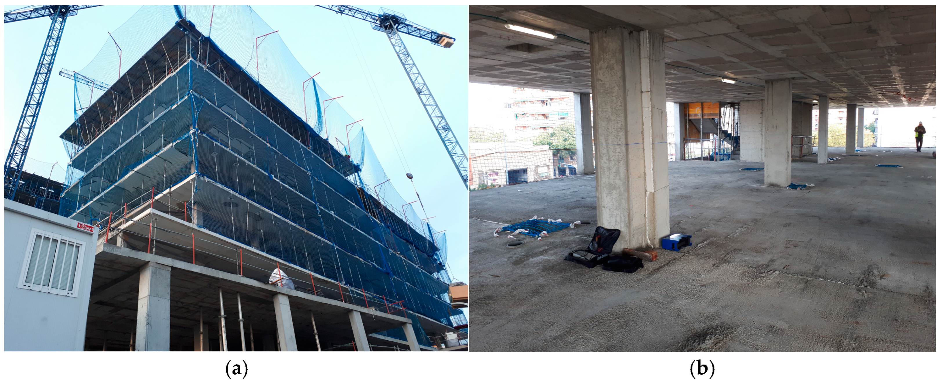
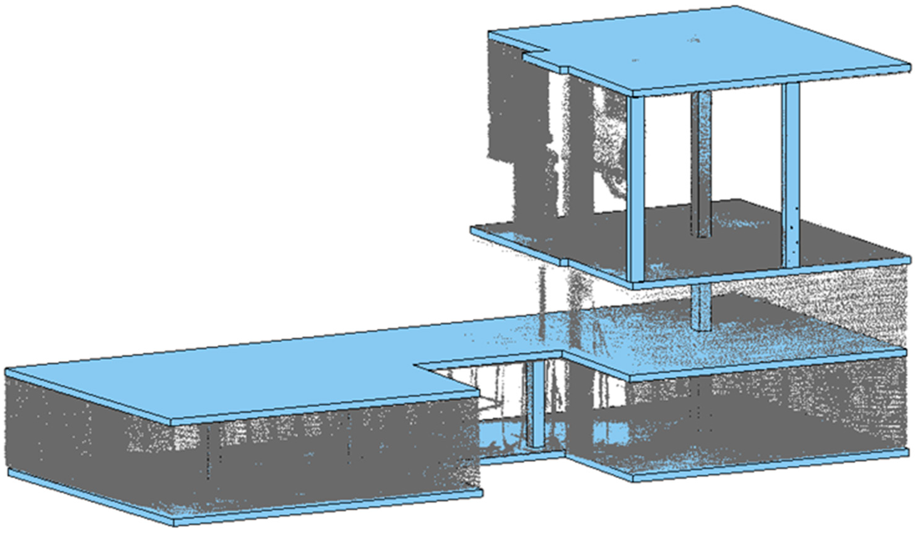
The proposed methodology was validated by applying it to two distinct scenarios within a residential building located in Badalona, Spain. The building features an asymmetrical U-shaped floor plan (Figure 5) and was under construction at the time of data acquisition, with a projected lifespan of 50 years. Covering an area of 25,000 m², the structure included two basement levels designated for parking, a ground floor intended for commercial offices, and upper levels allocated for residential housing. The building was divided into two sections: the north block, comprising 14 floors, and the south block, with 13 floors.

During data acquisition, the building was at various stages of construction, providing an opportunity to test the proposed methodology in diverse environments and varying levels of complexity. Three specific floors were chosen for the data collection. These floors were selected for their construction state and geometric complexity, making them representative of typical construction scenarios. The scenes included walls, pillars, floors, and ceilings. Additionally, the first floor included several metal props commonly used for shoring structures.

Data acquisition was conducted using the ground drone described in Section 3.1. For the first floor, 11 stations were required using the Stop&Go strategy, the second case study needed 7 stations to cover all areas, while the third floor required 8 stations. The first floor required more stations due to its construction stage (i.e., with several metal props), which resulted in more occlusions.

To balance data quality and acquisition efficiency, a 60% overlap between scans was set, with a scanning resolution of 4 mm at 20 m. This overlap was chosen to optimise the precision and reliability of the automatic alignment process. Additionally, points within 0.8 m of the ground drone (minimum acquisition range: 0.6 m) were excluded to ensure accurate data collection

Each scan position required approximately 3 min, plus additional time for movement between stops. The total acquisition time was 45 min for the first floor, 25 min for the second floor, and 30 min for the third floor.

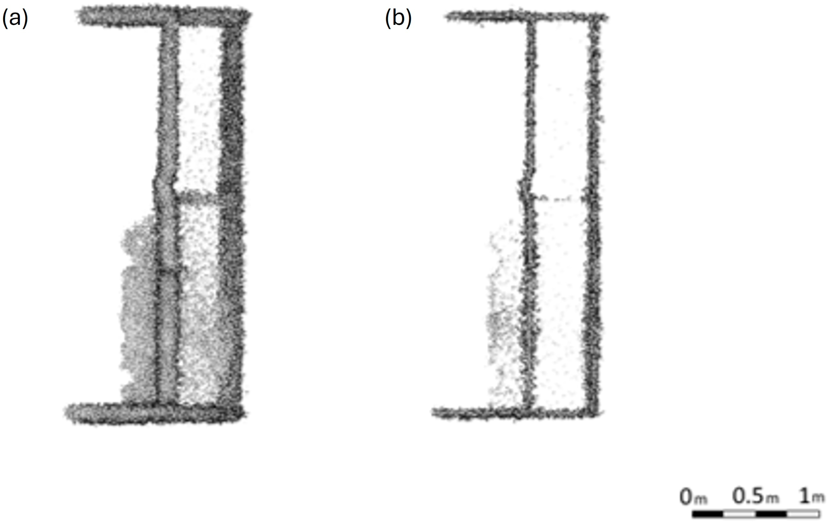
To ensure a clean and consistent dataset for the next steps, the raw point clouds were pre-processed with the anisotropic filtering as described in Section 3.2. The following input parameters were considered in the anisotropic filtering: $∆t=400, k=30, iterations=200$, resulting in a noise-free point cloud (Figure 6).

Analysing Figure 6 and the rest of the point clouds filtered, it seems clear that the application of anisotropic filtering significantly improved the quality of the point clouds by effectively reducing noise while preserving critical geometric features such as edges and corners. This enhancement is particularly evident in areas with high geometric complexity, where traditional filtering methods often blur or distort fine details. The resulting point clouds exhibit smoother transitions in homogeneous regions and sharper delineation in regions with abrupt changes, such as walls and structural joints. These improvements facilitate more accurate subsequent processing steps, such as the alignment and semantic classification, underscoring the suitability of anisotropic filtering for construction site data with varying levels of detail and noise.

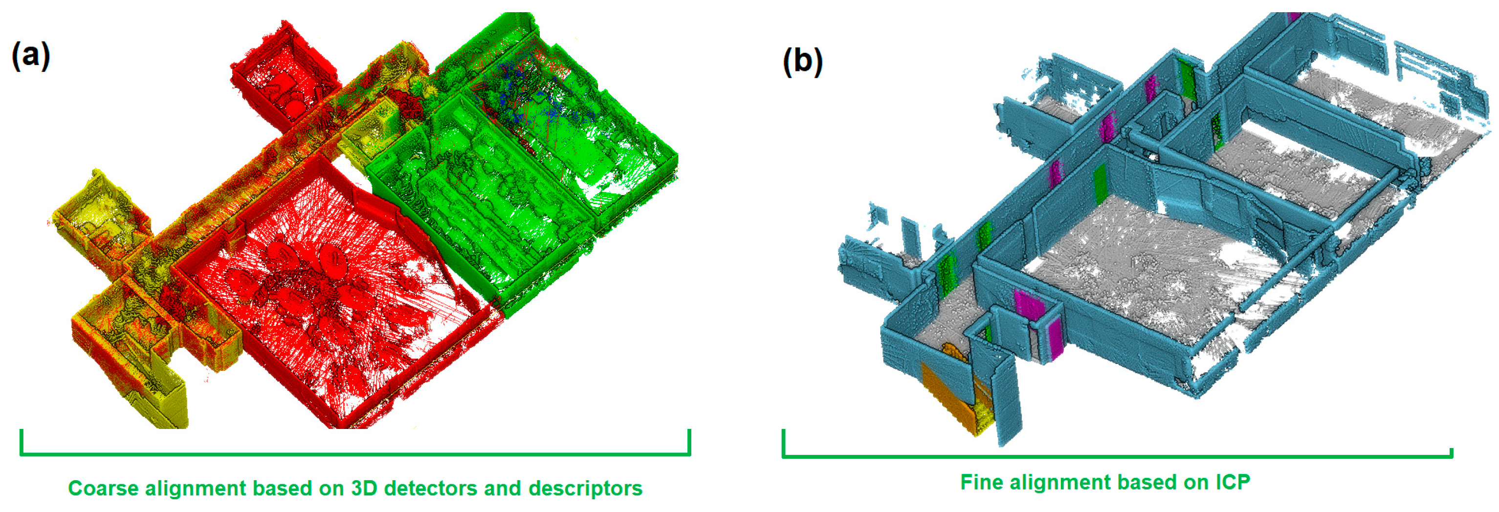
After the noise removal, point clouds were automatically aligned (Figure 7). The automatic alignment procedure outlined in Section 3.3 was applied separately to the different scans of each floor. The procedure included the following: (i) coarse registration, using the Harris 3D Noble detector and PFH descriptor; (ii) fine registration, using the ICP algorithm for adjusting the point clouds with millimetric precision.

With a unique point cloud filtered and aligned per floor, a semantic classification was performed using the deep learning network adapted and trained to construction works and described in Section 3.4. A custom architecture (Figure 8) was selected over existing models to accommodate better the case studies on semantic point cloud classification of buildings under construction. Although predefined models have demonstrated strong performance in various applications, they may not always be optimally suited for capturing the unique geometric and structural patterns present in construction sites. Particularly, the flexibility of our library allows layers to be dynamically added or removed, optimising performance based on specific project requirements and data constraints. This adaptability is particularly valuable when dealing with highly dynamic construction environments, where standard models may require additional fine-tuning or modifications to achieve comparable performance. Additionally, integrating this architecture into a dedicated library ensures seamless compatibility with previous developments while also facilitating future enhancements and scalability without external constraints. This approach does not dismiss the potential of existing models but rather provides an alternative pathway for improving adaptability and efficiency in the specific context of Scan-vs-BIM applications.

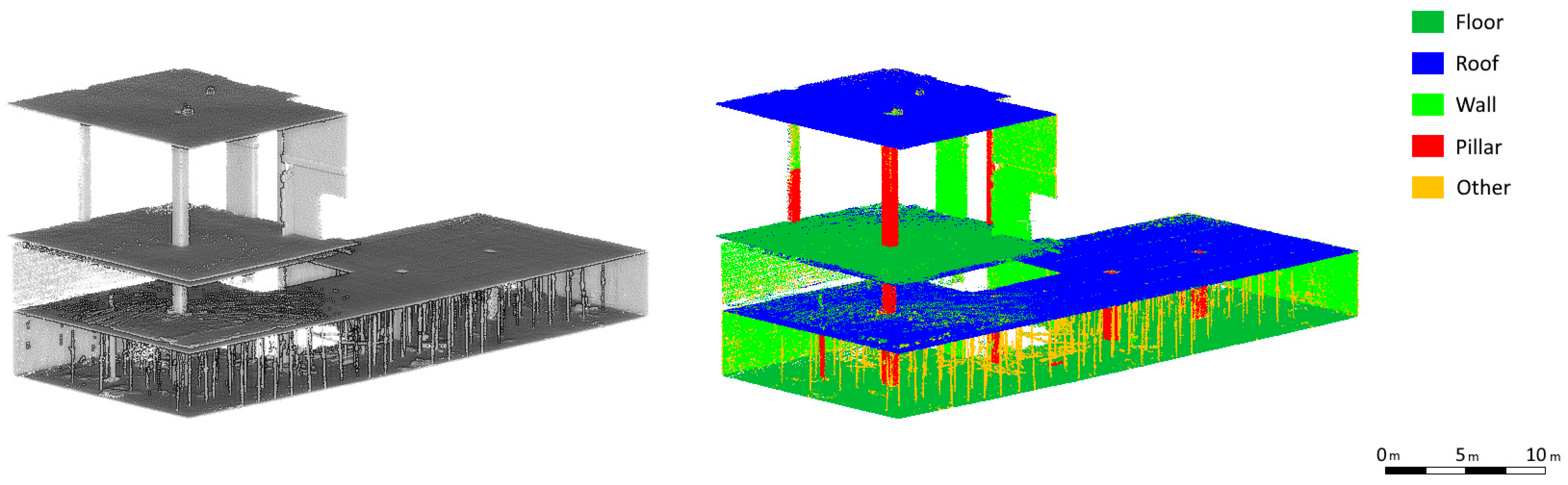
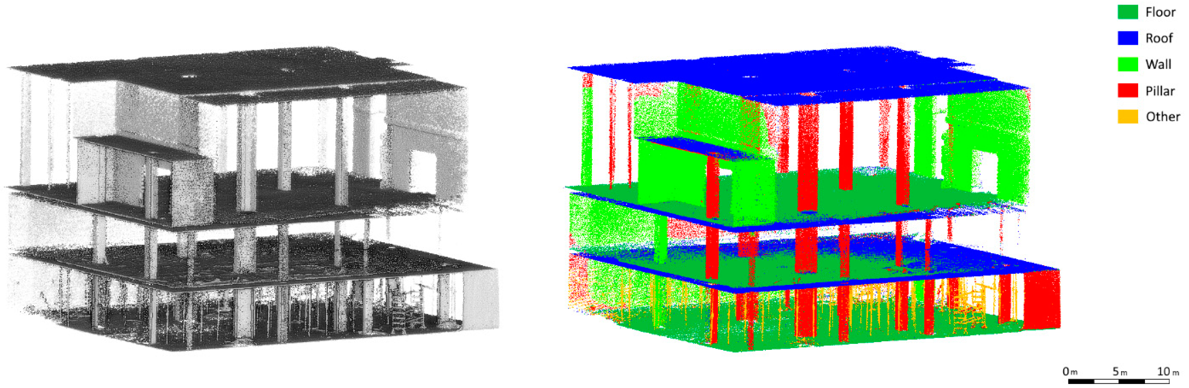
Figure 9 and Figure 10 show the point cloud with the implementation of semantic classification in which the most relevant elements of the construction such as floors, ceilings, walls, and pillars, as well as metal props used on the first floor, can be distinguished.

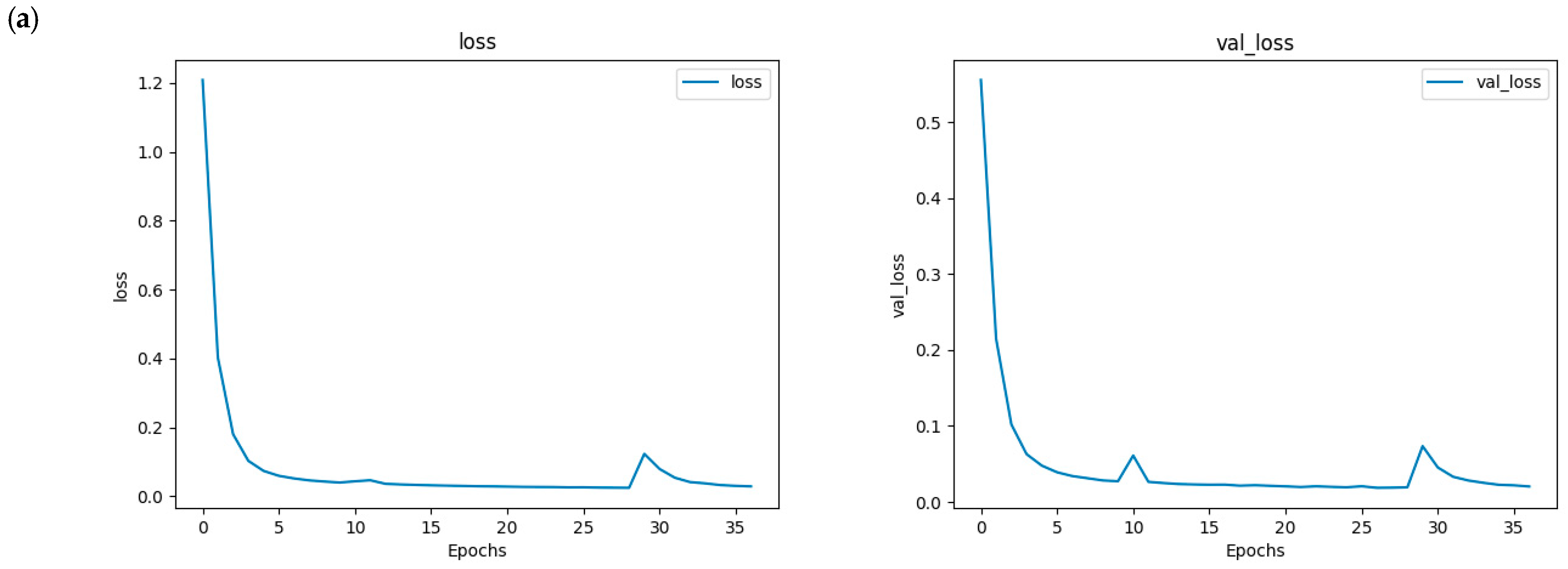
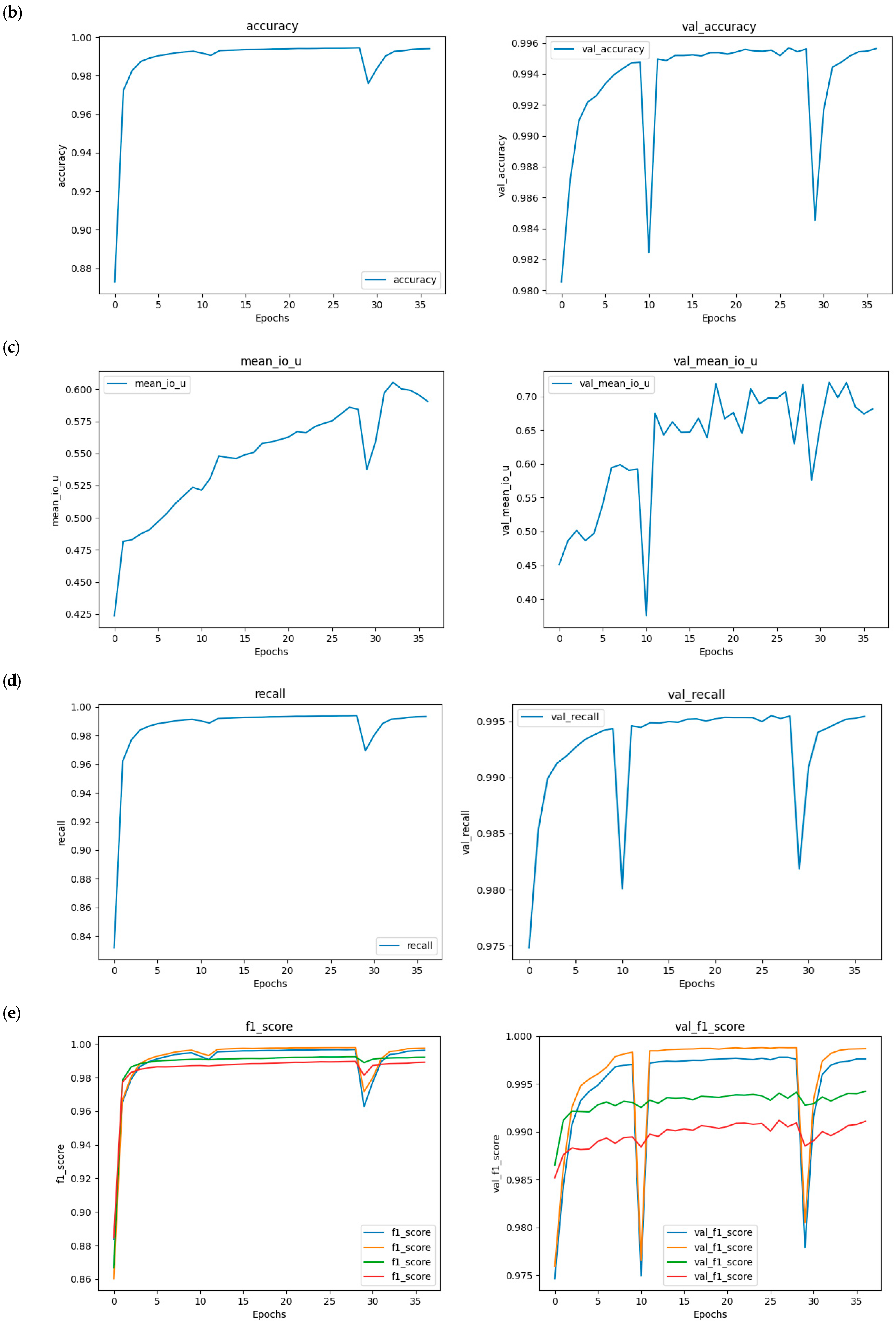
The model was trained using the Categorical Cross Entropy loss function, which is well suited for semantic segmentation tasks. The Adam optimisation algorithm was employed due to its efficiency and adaptability in adjusting the model’s weights during training. Additionally, the Early Stopping technique was implemented to halt training if no improvement in model performance was observed after 10 consecutive epochs. In this case, the model retains the configuration from the best-performing epoch, i.e., the one that achieved the highest performance before stagnation. The following statistical metrics (

Table 4. Statistical metrics obtained for the semantic classification in the best epoch.

	Loss	Accuracy	mIoU	Recall	F1 Score
Training	0.019	0.995	0.672	0.995	0.995
Validation	0.014	0.996	0.751	0.996	0.996

) and graphics (Figure 11) were obtained.

This performance underscores the network’s capacity to leverage geometric and contextual features unique to construction projects. Additionally, the network’s efficiency in processing large-scale point clouds ensures its applicability to real-world scenarios, enabling improved monitoring and decision-making throughout the construction process. These results validate the potential of neural networks as a reliable tool for advancing automated construction site analysis.

The results of the semantic classification demonstrate the effectiveness of the custom-designed neural network in accurately identifying and categorising structural elements within point clouds of buildings under construction. To ensure a comprehensive evaluation, the dataset used in this study consists of 2.6 million points captured from two distinct construction scenarios, representing varying levels of complexity, occlusions, and environmental conditions. The dataset was split into training and testing subsets, with 75% allocated for training and 25% for testing, ensuring a balanced distribution across all structural classes.

The network’s ability to generalise across diverse construction environments highlights its robustness. Key structural components such as walls, pillars, and ceilings were classified with high precision, even in cluttered and partially occluded areas typical of construction sites. The analysis of class distribution within the dataset further confirms that the model maintains consistent performance across both frequent and less-represented categories, mitigating potential class imbalance issues.

Additionally, the network’s efficiency in processing large-scale point clouds ensures its applicability to real-world scenarios, facilitating improved monitoring, quality control, and decision-making throughout the construction process. These results validate the potential of neural networks as a reliable tool for advancing automated construction site analysis, with a structured dataset evaluation that supports the reliability and generalizability of the approach.

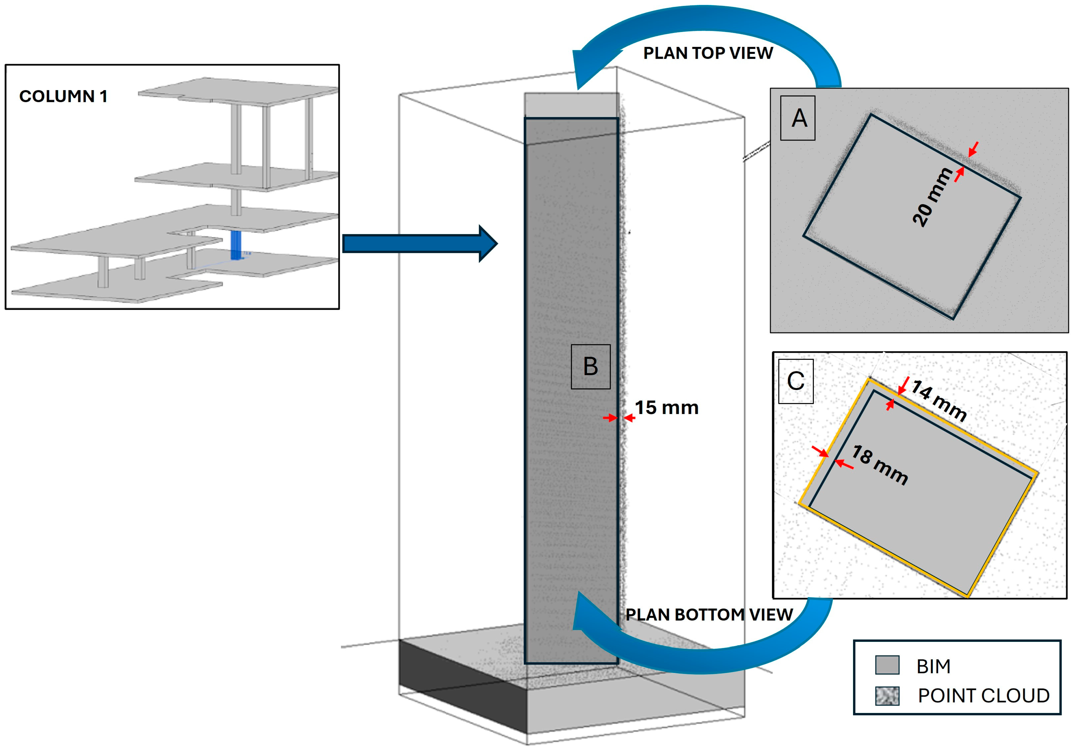
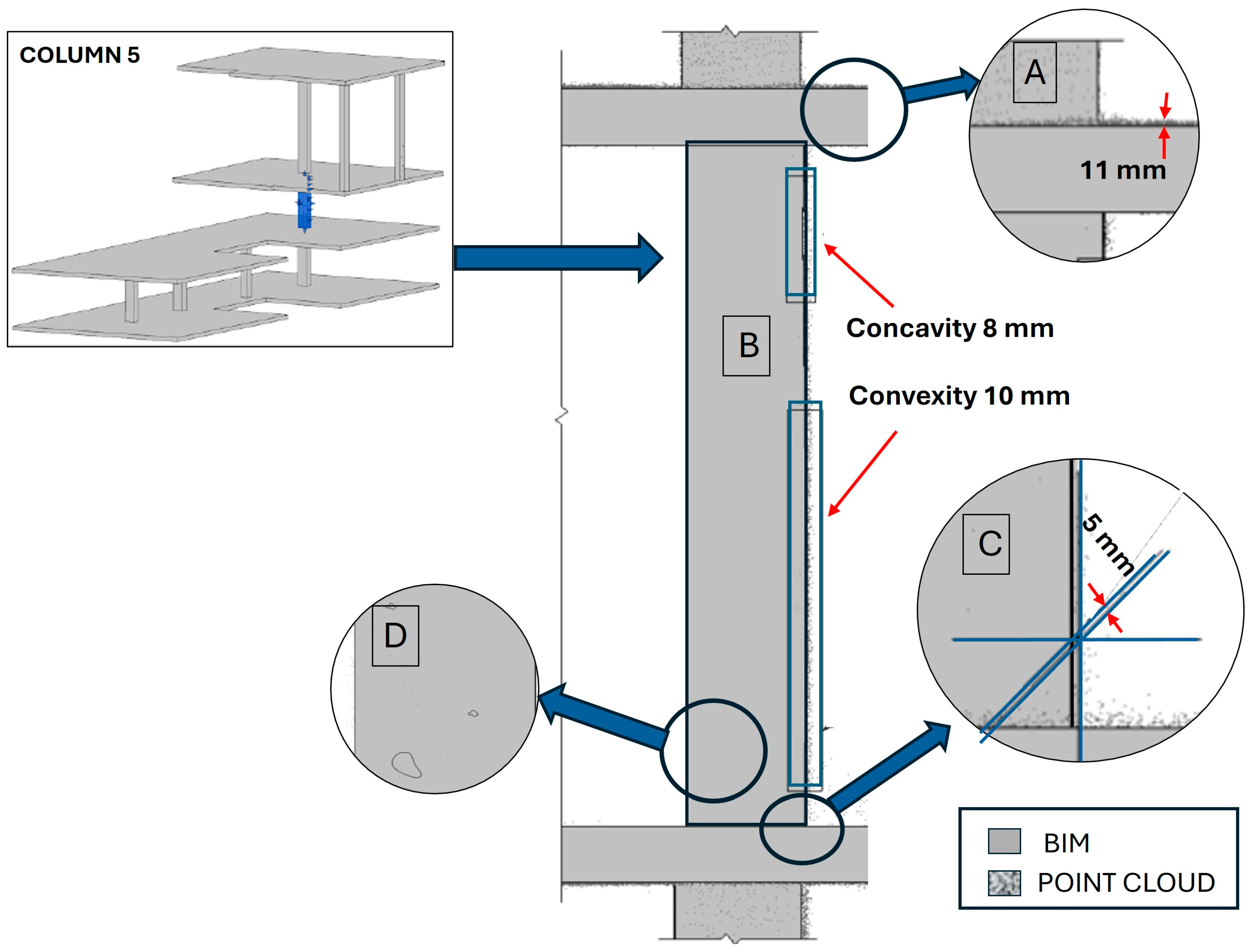
Once the point cloud data obtained by the ground drone was processed, it was compared with the theoretical BIM designed for this construction. The comparison of the two models, as-built vs. BIM, was carried out using Autodesk Revit 2024 software, which has modules that allow direct comparison of the two models. Figure 12 presents a comparison between the model obtained from the ground drone (as-built) and the BIM, focusing on the most relevant structural elements, specifically the concrete columns, to ensure the structural integrity of the building is properly assessed. The columns that make up the three-storey building were analysed quantitatively by measuring the discrepancies that exist between the two models in terms of the key geometry parameters of the columns. The comparison between the BIM and the as-built point cloud was conducted using specified criteria for translations, overhangs, levels, section variations, flatness, relative measurements, and voids. The established limits of the geometrical parameters are those that can be assumed so that there is no loss of compressive strength of the column that could endanger the structural integrity of the building. For the quantified parameters, the admissible limits have been applied to ensure the structural integrity and safety of the construction site, which are described below:

-

Translations from −24 mm to +12 mm: refer to the horizontal or vertical movement of the axis of the column from its design position.

-

Overhangs from −24 mm to +12 mm: refer to a change in the position of the upper part of the column relative to its base, when the upper part seems to ‘protrude’ or is displaced.

-

Levels from −20 mm to 20 mm: refer to vertical deviations of the column level (column elevation).

-

Section variation from −10 mm to 8 mm: refers to changes in the cross-sectional size of the column. For example, the section at the bottom of the column may differ from the section at the top of the column.

-

Flatness (3 m rule) from −12 mm to +12 mm: refers to how flat the surface of a column is along its entire length or height. The 3 m rule means that the measurement is made over a length of 3 m.

-

Relative measurements from −6 mm to +10 mm: refer to relative deviations that may pertain to the dimensional relationships between two or more columns or between different sections of the same column. For instance, this occurs when two columns are aligned at different levels with an overlap, yet they exhibit an offset, resulting in a misalignment where they do not coincide vertically.

-

Voids: refer to unexpected cavities in the column, which may result from construction or design errors.

The discrepancies obtained for the selected geometrical parameters are shown in Figure 13 and Figure 14. It can be seen from this table that there are small variations for most of the parameters, which are within the admissible limits.

The results of the comparison between the as-built point cloud data and the BIM demonstrate the efficacy of the proposed methodology in assessing the structural integrity of critical building components, particularly concrete columns. The discrepancies observed in geometric parameters, such as translations, overhangs, levels, and section variations, were within the established admissible limits, ensuring that the structural integrity of the building was not compromised. For instance, the detected translation discrepancy of 20 mm and the overhang of 20 mm were well within the tolerable ranges for structural safety. Similarly, variations in column cross-sections, flatness, and relative measurements were minor, reaffirming the accuracy of the construction relative to the design. While voids were observed in some columns, their presence highlights potential areas for improvement in concreting processes rather than structural concerns. Overall, these findings validate the integration of ground drone inspections with BIM-based analysis as a robust tool for monitoring and ensuring the quality and safety of construction projects. Specifically, integrating georeferenced and semantically enriched point cloud data directly into the BIM workflow proves to be far more efficient than traditional methods that require converting point clouds into a BIM through complex reverse engineering processes. These conventional approaches are not only time-consuming but also prone to errors, making direct point cloud integration a more reliable and accurate solution for real-time construction assessment.

5. Conclusions

This study introduces a comprehensive methodology for processing point cloud data obtained through ground drone inspections and comparing it with BIMs to identify and address discrepancies during the construction process. The proposed approach has proven effective in detecting deviations, particularly in critical structural elements, such as concrete columns, ensuring a higher level of precision and reliability in construction monitoring. Regarding the novel methodology developed for assessing construction buildings, the following aspects could be highlighted:

(i)

The integration of anisotropic filtering, automatic alignment, and semantic classification has proven to be a robust methodology for processing and analysing point cloud data in construction scenarios. Anisotropic filtering effectively reduces noise while preserving critical geometric features, enabling cleaner and more accurate data for subsequent processing. Automatic alignment, achieved through coarse and fine registration steps, ensures the precise positioning of point clouds within a unified coordinate system, minimizing manual intervention and errors. The incorporation of semantic classification further enhances the methodology by providing meaningful categorisation of structural elements in construction works, facilitating a detailed analysis and quality control. Together, these processes form a comprehensive pipeline that optimises point cloud processing, ensuring accurate model updates and contributing to the reliability of BIM-based construction audits.

(ii)

The Scan-vs-BIM methodology developed successfully identified discrepancies between both models, such as translation, section variation, level differences, and others. These discrepancies, while not compromising the overall structural integrity, highlight areas for improvement to enhance the accuracy of the BIM and better reflect actual site conditions.

(iii)

By applying this methodology across different construction phases, the study establishes a foundation for a digital twin approach that dynamically integrates real-time data with BIMs. This adaptability ensures that BIMs remain accurate throughout the construction cycle, addressing evolving site conditions and construction complexities. As a result, cost savings and efficiency can be provided to construction works, reducing the need for extensive manual inspections.

Future research can expand this methodology by incorporating a broader range of structural and non-structural elements, addressing challenges such as highly reflective surfaces, temporary site installations, and occluded components. A key direction will be the integration of multi-modal data sources, combining TLS with photogrammetry and thermal imaging to enhance point cloud classification accuracy and contextual awareness. Another critical area is the automation of corrective feedback within the Scan-vs-BIM workflow. Future developments should focus on real-time deviation analysis and rule-based decision support systems that can autonomously suggest corrections in BIM models. Implementing reinforcement learning mechanisms could allow the system to learn from past corrections, continuously refining classification accuracy and reducing false positives in anomaly detection.