Finite-Time Formation Control for Clustered UAVs with Obstacle Avoidance Inspired by Pigeon Hierarchical Behavior

Abstract

To address the formation control issue of multiple unmanned aerial vehicles (UAVs), a finite-time control scheme based on terminal sliding mode (TSM) is investigated in this paper. A quadcopter UAV with the vertical takeoff property is considered, with cascaded kinematics composed of rotational and translational loops. To strengthen the application in the low-cost UAV system, the applied torque is synthesized with an auxiliary rotational system, which can avoid utilizing direct attitude measurement. Furthermore, a terminal sliding mode surface is established and employed in the finite-time formation control protocol (FTFCP) as the driven thrust of multiple UAVs over an undirected topology in the translational system. To maintain the safe flight of the UAV clusters in an environment to avoid collision with obstacles or with other UAV neighbors, a pigeon-hierarchy-inspired obstacle avoidance protocol (PHOAP) is proposed. By imitating the interactive hierarchy that exists among the homing pigeon flocks, the collision avoidance scheme is separately enhanced to generate the repulsive potential field for the leader maneuver target and the follower UAV cluster. Subsequently, the collision avoidance laws based on pigeon homing behavior are combined with the finite-time sliding mode formation protocol, and the applied torque is attached as a cascaded structure in the attitude loop to synthesize an obstacle avoidance cooperative control framework. Finally, simulation scenarios of multiple UAVs to reach a desired formation among obstacles is investigated, and the effectiveness of the proposed approach is validated.

1. Introduction

The cooperative control of unmanned aerial vehicles (UAVs) has drawn significant research interests in both academia and industry [1,2]. The corresponding techniques in object detection [3,4], visual target tracking [5,6,7], optimal path planning [8,9,10], and coordinated control [11,12] are investigated, expecting to solve complex tasks in harsh environments. To ensure better convergence speed and strong robustness against disturbances, the finite-time control theory is proposed in the replacement of asymptotical stable control laws and implemented in various scopes of control applications. The quadrotor UAV is a mobile robot with vertical takeoff and landing properties and is typically used in three-dimensional multi-agent coordinative control verification [12]. Equipped with complex decoupled subsystems of attitude and position, respectively, cascaded control loops are employed in quadrotors, requiring the investigation of nonlinear control laws in both attitude and position system dynamics. In the control framework of multiple quadrotor UAVs, the negotiation mechanism between neighboring UAVs is challenging, currently introducing significant potential for promotion. Since there exist obstacles with unknown shapes and diverse levels of threat in practical UAV applications, obstacle avoidance techniques are required to guarantee collision-free formation control performance. A variety of obstacle avoidance methods are developed; however, for a cluster of UAVs, adoptable collision avoidance mechanisms have seen a lack of investigation. Since there exists much inspiration from the basic interactive principles of biological swarms, autonomous formation control approaches or intelligent cooperating rules can be potentially synthesized. In this section, the existing literature is demonstrated in three aspects below: collision avoidance methodologies, finite-time control and application, and bio-inspired mechanisms in UAV coordinated control issues.

There exist comprehensive studies that emphasize obstacle avoidance, mainly in scenarios of multi-agent consensus and unmanned robotic swarms. These proposed approaches can mainly be divided into the following categories: obstacle avoidance approaches based on the potential field (PF) gradient [13,14,15,16], path planning regulator [17,18,19], model predictive control [20,21,22], and vector field guidance [23,24]. In [25], the artificial potential field (APF) is employed on a fast terminal sliding mode surface, and both collision safety and obstacle avoidance in the formation control process are guaranteed. In [26], Lyapunov-like barrier function series are designed to be combined into a distributed control protocol to maintain a conflict-free formation safety control for quadrotor UAVs. In [27], a split–merge mechanism according to pigeons’ flocking behavior is embedded into the artificial potential field, and thus a steering controller to avoid obstacles is designed for multiple UAVs and validated through outdoor experiments. Apart from achieving obstacle-free control by combining the PF gradient with formation control laws, the PF is often integrated with path planning algorithms. In [28], an adaptive APF with global search adjustment is proposed and embedded with Rapidly Exploring Random Tree Star (RRT*) for solving the path planning and task assignment issues of multiple UAVs. In [29], both a novel repulsive coefficient and dynamic step-size-adjusting mechanism are introduced to build an improved APF, which is merged with RRT* and is proved to have optimal sampling direction and spatial distribution in the determination of the search path. Furthermore, a smooth shifting function and two collision-free functions are combined to construct a Lyapunov-based model predictive controller and applied to a UAV swarm in [30] in a spatial space. Then, in [31], a vector field is applied using the heading guidance law to attain collision-free formation among unmanned surface vessels.

The commonly used consensus control laws in our previous work only ensure that the error dynamic systems are asymptotically stable [32,33]. However, recent studies consider the newly designed Lyapunov functions to satisfy certain properties, resulting in system states converging into an ultimately bounded region within an upper time bound that corresponds to the initial system state, namely finite-time (FT) convergence. In [34], a desired formation can be maintained through the decentralized FT observer and control law. In [35], a distributed neural-network-based nonsingular fast terminal sliding mode controller is proposed to guarantee FT stability for multiple unmanned surface vehicles. In [36], an event-triggered FT formation control protocol is established under a disturbance estimated by extended state observers.

Animals in the wild such as hawks, wolves, lions, and pigeons often spontaneously form groups to achieve coordination in hunting or evasion behavior. Some of those inspiring animal behaviors are similar to robotic swarms in several aspects, especially in agent translational kinematics as well as alignment and repulsive interactions among neighboring individuals [37]. In [38], the hierarchical social structure and robust interaction patterns of grey wolves are taken into consideration. Then, a bio-inspired adaptive formation consensus protocol is synthesized. Motivated by the chasing and anti-attack behavior in groups of coyotes, elks, and wolves, a set of energy game models are established in [39]. The sheepdog assignment for the sheep-herding task is considered the fundamental inspiration in [40], and the steering control laws are designed with the biological behavior of sheep herding, including aggregation and dispersion, and are validated through a wheeled robotic swarm. As a typical animal species that is well-known for its collective behavior when flying in flocks, pigeons have attracted widespread attention in the investigation of biomimicry [41].

In a leader–follower interactive topology, trajectories for the leader are commonly determined by the system settings, and the followers are anticipated to form a desired formation pattern around the leader node. If the obstacles are distributed near the predefined trajectory, then the UAV clusters, especially the leader UAV, are blocked. Since the leader trajectory is set to be collision-free in the existing literature, collision avoidance protocols should be investigated for both the leader and followers in this work. Additionally, obstacle avoidance and the neighboring collision-free formation are required to be maintained at the same time. For the sake of combination with the formation control term, the collision-free controller is designed as a gradient-based form differentiated from the energy potential function. Therefore, a potential-field-based collision avoidance law inspired by the pigeon hierarchy principle is developed in this paper, resulting in guaranteeing cooperative collision evasion for the leader–follower formation.

In this paper, the leader–follower collision-free coordination framework is developed in three modules. An attitude consensus stabilization law composed of auxiliary error system is proposed at first to avoid the direct state feedback; namely, the applied torque can be synthesized without the quaternion and rotational angle measurement feedback while only introducing the auxiliary state error. Secondly, a pigeon-hierarchy-inspired leader–follower collision avoidance protocol for the leader and follower, respectively, is proposed, achieving coordinated and safe collision avoidance when meeting obstacles blocking the leader’s trajectory. Thirdly, a finite-time terminal sliding mode collision-free formation and reconfiguration control law is proposed by synthesizing the first two modules, attaining finite-time reconfiguration convergence.

To overcome the dilemma in designing control laws for the strong coupling kinematics in the clustered quadcopter UAV system, the cooperative formation-tracking scheme with obstacle avoidance is investigated in this paper. The main contributions are discussed as follows:

• An auxiliary error system is established to achieve collaborative attitude convergence without direct state feedback in quaternion, rotation angles, and angular velocity, but the applied torque in the attitude consensus law is synthesized only by utilizing state-tracking errors or auxiliary errors. Aiming at reaching convergence in the attitude loop, an attitude consensus stabilization law (ACSL) is established by combining the adaptive angular rate command and the auxiliary error system to produce an applied torque, and thus cooperative attitude tracking can be reached under arbitrary initial quaternion and angular rate settings.
• Inspired by the homing behavior of pigeon flocks, a pigeon-hierarchy-inspired collective obstacle avoidance protocol (PHOAP) is proposed in a hierarchical scheme. The energy function of the PF is designed to provide the repulsive control force for collision safety between UAVs and for obstacle avoidance. The leader target is driven by the obstacle repulsive protocol to regulate an appropriate trajectory. However, the follower UAVs are guided to track the desirable leader’s trajectories while achieving cooperative obstacle avoidance.
• A terminal sliding mode (TSM) surface is developed based on lumped translational errors. Moreover, a finite-time formation control protocol (FTFCP) is elaborated by using the combination of TSM to guarantee formation consensus tracking within an upper finite-time bound related to the initial states in the translational loop. To synthesize the ACSL, the PHOAP, and the FTFCP based on TSM, the cooperative formation control and obstacle avoidance framework is attained and validated through typical simulation scenarios in this paper.

The rest of this paper is organized as follows. Section 2 provides the preliminaries of graph theory and fundamental notation. The modeling of the UAV and the control objectives are also discussed. Section 3 presents the controller design and provides the stability proof. Section 4 displays the numerical simulation results, and Section 5 summarizes the whole work.

2. Preliminaries and Problem Formulation

2.1. Preliminaries

First, a few significant notations and symbols: $ℝ$, ${ℝ}_{+}$, ${ℝ}^n$, and ${ℝ}^{m\times n}$ represent the fields of real numbers, positive real numbers, $n$-dimensional ($n$-D) column vectors, and matrixes of $m$ rows and $n$ columns, respectively. Subsequently, $\mathbb{Z}$, ${\mathbb{Z}}_{+}$, ${\mathbb{Z}}^n$, and ${\mathbb{Z}}^{m\times n}$ are the same for integers. For a vector $a={\left[a_1,a_2,a_3\right]}^T\in {ℝ}^3$, the 1-norm and 2-norm are separately denoted by ${‖a‖}_1={\displaystyle \sum _{i=1}^n\left|a_i\right|}$ and ${‖a‖}_2={\displaystyle \sum _{i=1}^n{\left(a_i\right)}^2}$. Additionally, the power of a vector is ${〈a〉}^h={\left[{\left(a_1\right)}^h,{\left(a_2\right)}^h,{\left(a_3\right)}^h\right]}^T$. For the sliding mode design, the sign function is denoted as $\mathrm{sgn}\left(a\right)={\left[\mathrm{sgn}\left(a_1\right),\mathrm{sgn}\left(a_2\right),\mathrm{sgn}\left(a_3\right)\right]}^T$, while the signum function is depicted as $si{g}^k\left(a\right)={\left[{\left|a_1\right|}^k\mathrm{sgn}\left(a_1\right),{\left|a_2\right|}^k\mathrm{sgn}\left(a_2\right),{\left|a_3\right|}^k\mathrm{sgn}\left(a_3\right)\right]}^T$. For ease of expression, the two terms above are represented by $\mathrm{sgn}\left(a\right)={\left[\mathrm{sgn}\left(a_i\right)\right]}_{i=1,2,3}^T$ and $si{g}^k\left(a\right)={\left[{\left|a_i\right|}^k\mathrm{sgn}\left(a_i\right)\right]}_{i=1,2,3}^T$. The skew-symmetric matrix for a vector $a\in {ℝ}^3$ is defined as $a_{\times }=\left[0,-a_3,a_2;a_3,0,-a_1;-a_2,a_1,0\right]$. The operator $\otimes$ represents the Kronecker product.

Since a leader–follower scheme is investigated, the interactive topology in this paper is divided into two layers. The first layer, that is, the topology between followers, is considered to be undirected, denoted as $\mathsf{𝒢}=\left\{\mathsf{𝒱},\epsilon \right\}$, where $\mathsf{𝒱}=\left\{i\left|i\in {\mathbb{Z}}_{+},1\le i\le N\right.\right\}$ is the vertex set and $\epsilon \subseteq \mathsf{𝒱}\times \mathsf{𝒱}$ is the edge set. If an edge from node $i$ to node $j$ exists, namely $〈j,i〉\in \epsilon$, then $〈i,j〉\in \epsilon$ holds for an undirected graph. Moreover, the Laplacian matrix of $\mathsf{𝒢}\mathrm{is}L={\left[l_{ij}\right]}_{i,j=1,\dots N}$, whose $i$-th diagonal element is $l_{ii}={\displaystyle {\sum }_{j=1,j\ne i}^N{w}_{ij}}$, and $l_{ij}=-w_{ij}$ at other locations. However, the information is regulated to be transferred in a fixed direction from the leader vertex to the followers under the second layer. Subsequently, the link weights are depicted by $B=\mathrm{diag}{\left\{b_{i0}\right\}}_{i=1,\dots N}$ with $b_{i0}>0$ representing that the link from the leader to follower node $i$ exists. The augmented Laplacian matrix is defined as $M=L+B$.

Assumption 1. 

There exists at least one follower UAV that has access to the states of the leader vertex, namely $\exists i\in \mathsf{𝒱},s.t. b_{i0}>0$. Under such circumstances, the augmented Laplacian matrix is guaranteed to be positive and definite [36].

The following theories are significant for the formation controller development in the translational loop of the UAV system.

Definition 1. 

Consider a nonlinear system whose dynamics are $\dot{x}\left(t\right)=F\left(t,x\left(t\right)\right)$, with system state $x\left(t\right)\in \mathsf{𝒟}\subseteq {ℝ}^n$, $x\left(t_0\right)=x_0$, and $F:\mathsf{𝒟}\to {ℝ}^n$. If there exists a function denoted as $T\left(x_0,ƛ\right):\mathsf{𝒟}\times {ℝ}_{+}\to {ℝ}_{+}$ related to the initial state $x_0$ and a positive constant $ƛ>0$ that can guarantee that ${‖x\left(t_0\right)‖}_2<ƛ$ holds for any $t\in \left[t_0+T\left(x_0,ƛ\right),+\infty \right)$, then the system is locally practically finite-time stable. Furthermore, if $\mathsf{𝒟}={ℝ}^n$, then the system is globally practically finite-time stable [42].

Lemma 1. 

For the system $\dot{x}\left(t\right)=F\left(t,x\left(t\right)\right)$, if we can find a positive definite function $V\left(t,x\left(t\right)\right):{ℝ}_{+}\times {ℝ}^n\to {ℝ}_{+}$ that is continuous in its domain and for which the inequality $\dot{V}\left(t,x\left(t\right)\right)\le -\alpha V^p\left(t,x\left(t\right)\right)-\beta V\left(t,x\left(t\right)\right)+\mathcal{l}$ holds for $\alpha >0$, $\beta >0$, $0<p<1$ and $\mathcal{l}>0$, then the system is consequently globally and practically finite-time stable [42].

Lemma 2. 

To avoid the singularity of the rotation matrix, a quaternion is introduced to be $Q_i={\left[{\vartheta }_i,q_i^T\right]}^T$, where ${\vartheta }_i\in ℝ$ and $q_i\in {ℝ}^3$. The inversion of a quaternion is defined in this paper as $Q_i^{-1}={\left[{\vartheta }_i,-q_i^T\right]}^T$. Moreover, the relative deviation of two quaternions $Q_i$ and $Q_j$ is defined by $Q_{ij}=Q_j^{-1}\odot Q_i=\left[{\vartheta }_j{\vartheta }_i+q_j^T{q}_i,{\vartheta }_j{q}_i^T-{\vartheta }_i{q}_j^T+q_i^T{\left(q_j\right)}_{\times }\right]$. The translation from a quaternion to a rotation matrix is denoted as $R\left(Q_i\right)=\left({\vartheta }_i^2-q_i^T{q}_i\right)I_3+2q_i{q}_i^T-2{\vartheta }_i{\left(q_i\right)}_{\times }$ [43].

2.2. Mathematical Model of UAV Cluster and Obstacle

The agent for the formation control issue in this paper is a quadcopter UAV. Since it is required to take off and land vertically, the system dynamics are often separated into two cascaded subsystems, that is, a rotational system and a translational system. The states of the rotational subsystem consist of the quaternion, angular velocity, and rotational matrix, denoted as $Q_i={\left[{\vartheta }_i,q_i^T\right]}^T\in {ℝ}^4$ where ${\vartheta }_i\in ℝ$ and $q_i\in {ℝ}^3$, ${\omega }_i\in {ℝ}^3$, and $R\left(Q_i\right)\in {ℝ}^{3\times 3}$, respectively. Moreover, the states in the translational system contain $p_i\in {ℝ}^3$ and $v_i\in {ℝ}^3$. For any $i\in \mathsf{𝒱}$, the follower UAV system dynamics are established as [44]

$$\left\{\begin{array}{l}{\dot{Q}}_i={\displaystyle \frac{1}{2}}\gamma \left(Q_i\right){\omega }_i\begin{array}{c}\\ \end{array}\\ \dot{R}\left(Q_i\right)=R\left(Q_i\right){\left({\omega }_i\right)}_{\times }\\ {\mathit{\Lambda }}_i{\dot{\omega }}_i=-{\left({\omega }_i\right)}_{\times }{\mathit{\Lambda }}_i{\omega }_i+{\tau }_i\begin{array}{c}\\ \end{array}\end{array}\right.$$

(1)

$$\left\{\begin{array}{l}{\dot{p}}_i=v_i\\ {\dot{v}}_i=-g{e}_3+{\displaystyle \frac{T_i}{m_i}}R\left(Q_i\right)e_3\end{array}\right.$$

(2)

where (1) and (2) are, separately, the rotational and translational updating laws of the UAV system differential equations, $\gamma \left(Q_i\right)={\left[-q_i,{\vartheta }_i{I}_3-{\left(q_i\right)}_{\times }\right]}^T\in {ℝ}^{4\times 3}$ is the quaternion updating matrix, $g$ is the gravitational acceleration, $T_i$ is the driven thrust, $m_i$ is the mass of the rotorcraft, and $e_3={\left[0,0,1\right]}^T$. The applied torque ${\tau }_i$ and the thrust $T_i$ need to be designed to maintain the stability of each UAV platform.

For the obstacle avoidance issue discussed in this paper, the effective region of the $k$-th obstacle and the detection region of the $i$-th UAV are separately defined as

$$\left\{\begin{array}{l}{\mathcal{C}}_k=\left\{x\in {ℝ}^3\left|‖x-o_k‖\le R_k^o,o_k\in {ℝ}^3,k\in \mathsf{𝒪}\right.\right\}\\ {\mathsf{𝒟}}_i=\left\{x\in {ℝ}^3\left|‖x-p_i‖\le R^d,p_i\in {ℝ}^3,i\in \mathsf{𝒩}\right.\right\}\end{array}\right.$$

(3)

where ${\mathcal{C}}_k$ represents the collision area of the $k$-th obstacle and ${\mathsf{𝒟}}_i$ denotes the detection scope of the $i$-th UAV, $o_k$ is the center position of the $k$-th obstacle, and $R^d$ and $R_k^o$ refer to the detection radius and the obstacle radius, respectively. It is obvious in (3) that the detection region of a UAV node is assumed to be a limited circular area.

Based on the definitions above, the obstacles detected by the $i$-th UAV node are summarized in a set as

$${\mathsf{𝒪}}_i=\left\{k\in \mathsf{𝒪}\left|‖p_i-o_k‖-R_k^o\le R^d,i\in \mathsf{𝒩}\right.\right\}$$

(4)

2.3. Problem Formulation and Control Objectives

The translational command control input is defined as $u_i=T_{i}R\left(Q_{c,i}\right)e_3/m_i$, and similarly to the previous work [32,44], $R\left(Q_{e,i}\right)={\left(R\left(Q_{c,i}\right)\right)}^{T}R\left(Q_i\right)$ is considered the rotation error matrix, where $R\left(Q_{c,i}\right)$ is the command rotation matrix as shown by (11) in [44]. The expression of $u_i$ and $R\left(Q_{c,i}\right)$ is substituted into the velocity dynamics in (2), thus obtaining ${\dot{v}}_i=-g{e}_3+u_i+{\displaystyle \frac{T_i}{m_i}}R\left(Q_{c,i}\right)\left(R\left(Q_{e,i}\right)-I_3\right)e_3$. For any $i\in \mathsf{𝒱}$, the position- and velocity-tracking errors are defined as $e_i^p=p_i-p_0-{\delta }_i$ and $e_i^v=v_i-v_0$, respectively, where ${\delta }_i$ denotes the formation offset of the i-th UAV, and $p_0$ and $v_0$ refer to the position and velocity of the maneuvering leader with simple dynamics as

$$\left\{\begin{array}{l}{\dot{p}}_0=v_0\\ {\dot{v}}_0=u_0\end{array}\right.$$

(5)

Due to the requirement of suppressing the translational formation-tracking errors, the differential equations for the translational errors are elaborated as

$$\left\{\begin{array}{l}{\dot{e}}_i^p=e_i^v\\ {\dot{e}}_i^v=-g{e}_3-{\dot{v}}_0+u_i+{\displaystyle \frac{T_i}{m_i}}R\left(Q_{c,i}\right)\left(R\left(Q_{e,i}\right)-I_3\right)e_3\end{array}\right.$$

(6)

When $R\left(Q_{e,i}\right)={\left(R\left(Q_{c,i}\right)\right)}^{T}R\left(Q_i\right)$ holds, the angular-rate-tracking error is defined as ${\omega }_{e,i}={\omega }_i-{\left(R\left(Q_{e,i}\right)\right)}^T{\omega }_{c,i}$, with ${\omega }_{c,i}$ being the command angular rate. Substituting it into (1), the error dynamics for the rotational loop are subsequently derived as

$$\left\{\begin{array}{l}\dot{R}\left(Q_{e,i}\right)=R\left(Q_{e,i}\right){\left({\omega }_{e,i}\right)}_{\times }\\ {\mathit{\Lambda }}_i{\dot{\omega }}_{e,i}=-{\left({\omega }_i\right)}_{\times }{\mathit{\Lambda }}_i{\omega }_i+{\tau }_i+{\mathit{\Lambda }}_i\left[{\left({\omega }_{e,i}\right)}_{\times }{\left(R\left(Q_{e,i}\right)\right)}^T{\omega }_{c,i}-{\left(R\left(Q_{e,i}\right)\right)}^T{\dot{\omega }}_{c,i}\right]\end{array}\right.$$

(7)

The main objectives in this paper can be divided into three cascaded parts, that is, to reach asymptotic convergence in the attitude loop, to ensure the practical finite-time stability of the translational loop, and to simultaneously avoid conflict between neighboring UAVs and collision with obstacles. In the attitude subsystem, $\underset{t\to \infty }{\lim }R\left(Q_{e,i}\right)=I_3$ and $\underset{t\to \infty }{\lim }{\omega }_{e,i}=0_3$ are required, and in the translational subsystem $\underset{t\to \infty }{\lim }{e}_i^p=0_3$ and $\underset{t\to \infty }{\lim }{e}_i^v=0_3$ are demanded for each $i\in$ to guarantee formation tracking when the UAV cluster is not influenced by any obstacles. However, when there exist obstacles, $‖p_i-p_j‖\ge \iota$ and $‖p_i-o_k‖-R_k^o\ge \iota$ are the safety constraints for $i,j\in \mathsf{𝒱}\cup \left\{0\right\}$, with an infinitesimal constant $\iota$ as the lower bound of the relative distance.

3. Main Results

In this section, the formation control laws and collision-free protocols are elaborated. Meanwhile, the detailed stability analysis is conducted for the attitude control laws and the translational formation control laws according to Lyapunov theories.

3.1. Attitude-Consensus-Tracking Protocol with Auxiliary System

Due to constraints in deriving the direct state feedback in the attitude system, auxiliary attitude error systems and adaptive command filter are elaborated in this section for achieving attitude stabilization with the lack of system state feedback. Therefore, the applied torque is developed by utilizing the relative quaternion obtained from monocular cameras or lasers to obtain relative information or by acquiring the attitude signal-tracking errors from onboard flight controller.

The auxiliary quaternion command is defined as $Q_{\beta ,i}={\left[{\vartheta }_{\beta ,i},q_{\beta ,i}^T\right]}^T$, with ${\vartheta }_{\beta ,i}\in ℝ$ and $q_{\beta ,i}\in {ℝ}^3$. Similar to the quaternion-tracking error $Q_{e,i}=Q_{c,i}^{-1}\odot Q_i$, the auxiliary quaternion error is proposed as ${\tilde{Q}}_{e,i}=Q_{\beta ,i}^{-1}\odot Q_{e,i}$ by utilizing the auxiliary quaternion command. According to Lemma 2, the auxiliary rotation error matrix can be derived as $R\left({\tilde{Q}}_{e,i}\right)={\left(R\left(Q_{\beta ,i}\right)\right)}^{-1}R\left(Q_{e,i}\right)$. Subsequently, an adaptive auxiliary command angular velocity ${\beta }_i$ follows the updating law as

$${\dot{\beta }}_i=-{\lambda }_i{\beta }_i+R\left({\tilde{Q}}_{e,i}\right){\overline{\tau }}_i$$

(8)

An auxiliary angular velocity error is defined in the same form of ${\omega }_{e,i}$ as ${\tilde{\omega }}_{e,i}={\omega }_{e,i}-{\left(R\left({\tilde{Q}}_{e,i}\right)\right)}^T{\beta }_i$. The expression ${\omega }_i={\omega }_{e,i}+{\left(R\left(Q_{e,i}\right)\right)}^T{\omega }_{c,i}$ and ${\omega }_{e,i}={\tilde{\omega }}_{e,i}+{\left(R\left({\tilde{Q}}_{e,i}\right)\right)}^T{\beta }_i$ are substituted into (7), and $\left(a_{\times }\right)a=0$ is employed. Since the newly designed variables of the auxiliary system are proposed, the auxiliary attitude error dynamics are depicted as

$$\dot{R}\left({\tilde{Q}}_{e,i}\right)=R\left({\tilde{Q}}_{e,i}\right){\left({\tilde{\omega }}_{e,i}\right)}_{\times }$$

(9)

$$\begin{array}{ll}{\mathit{\Lambda }}_i{\dot{\tilde{\omega }}}_{e,i}=& -{\left({\tilde{\omega }}_{e,i}\right)}_{\times }{\mathit{\Lambda }}_i{\tilde{\omega }}_{e,i}-{\left[{\left(R\left({\tilde{Q}}_{e,i}\right)\right)}^T{\beta }_i+{\left(R\left(Q_{e,i}\right)\right)}^T{\omega }_{c,i}\right]}_{\times }{\mathit{\Lambda }}_i{\tilde{\omega }}_{e,i}\\ & -{\left({\tilde{\omega }}_{e,i}\right)}_{\times }{\mathit{\Lambda }}_i\left[{\left(R\left({\tilde{Q}}_{e,i}\right)\right)}^T{\beta }_i+{\left(R\left(Q_{e,i}\right)\right)}^T{\omega }_{c,i}\right]\\ & -{\left[{\left(R\left({\tilde{Q}}_{e,i}\right)\right)}^T{\beta }_i+{\left(R\left(Q_{e,i}\right)\right)}^T{\omega }_{c,i}\right]}_{\times }{\mathit{\Lambda }}_i\left[{\left(R\left({\tilde{Q}}_{e,i}\right)\right)}^T{\beta }_i+{\left(R\left(Q_{e,i}\right)\right)}^T{\omega }_{c,i}\right]\\ & +{\tau }_i-{\mathit{\Lambda }}_i{\left({\left(R\left(Q_{e,i}\right)\right)}^T{\omega }_{c,i}+{\left(R\left({\tilde{Q}}_{e,i}\right)\right)}^T{\beta }_i\right)}_{\times }{\tilde{\omega }}_{e,i}\\ & -{\mathit{\Lambda }}_i{\left({\left(R\left(Q_{e,i}\right)\right)}^T{\omega }_{c,i}\right)}_{\times }\left({\left(R\left({\tilde{Q}}_{e,i}\right)\right)}^T{\beta }_i\right)-{\mathit{\Lambda }}_i\left({\left(R\left(Q_{e,i}\right)\right)}^T{\dot{\omega }}_{c,i}+{\left(R\left({\tilde{Q}}_{e,i}\right)\right)}^T{\dot{\beta }}_i\right)\end{array}$$

(10)

Moreover, the applied torque is synthesized with two terms: one is to guarantee the coordination of attitude tracking, while the other aims to compensate for the remaining items in (10), which are indicated by

$$\begin{array}{l}{\tau }_i={\stackrel{⌢}{\tau }}_i+{\overline{\tau }}_i\\ {\stackrel{⌢}{\tau }}_i={\mathit{\Lambda }}_i\left[{\left(R\left(Q_{e,i}\right)\right)}^T{\dot{\omega }}_{c,i}+{\left(R\left({\tilde{Q}}_{e,i}\right)\right)}^T{\dot{\beta }}_i\right]+{\mathit{\Lambda }}_i{\left({\left(R\left(Q_{e,i}\right)\right)}^T{\omega }_{c,i}\right)}_{\times }\left({\left(R\left({\tilde{Q}}_{e,i}\right)\right)}^T{\beta }_i\right)\\ \hspace{1em}\hspace{1em}+{\left({\left(R\left(Q_{e,i}\right)\right)}^T{\omega }_{c,i}+{\left(R\left({\tilde{Q}}_{e,i}\right)\right)}^T{\beta }_i\right)}_{\times }{\mathit{\Lambda }}_i\left({\left(R\left(Q_{e,i}\right)\right)}^T{\omega }_{c,i}+{\left(R\left({\tilde{Q}}_{e,i}\right)\right)}^T{\beta }_i\right)\\ {\overline{\tau }}_i=-k_{p,i}{q}_{e,i}-{\displaystyle \sum _{j\in {\mathsf{𝒩}}_i}{k}_{p,ij}{q}_{ij}}\end{array}$$

(11)

where $q_{ij}$ is the vector term of the relative quaternion $Q_{ij}$. A remark is proposed here for the computation of $Q_{ij}$ as

$$Q_{ij}=Q_j^{-1}\odot Q_i=\left(Q_j^{-1}\odot Q_{c,i}\right)\odot \left(Q_{c,i}^{-1}\odot Q_i\right)=Q_{e,j}^{-1}\odot Q_{e,i}$$

(12)

The quaternion-tracking error $Q_{e,i}$ is updated by

$${\dot{Q}}_{e,i}={\displaystyle \frac{1}{2}}\gamma \left(Q_{e,i}\right){\omega }_{e,i}$$

(13)

where the matrix $\gamma \left(Q_{e,i}\right)={\left[-q_{e,i},{\vartheta }_{e,i}{I}_3-{\left(q_{e,i}\right)}_{\times }\right]}^T$, and thus the two differential equations are obtained as

$${\dot{\vartheta }}_{e,i}=-{\displaystyle \frac{1}{2}}{q}_{e,i}^T{\omega }_{e,i}, {\dot{q}}_{e,i}={\displaystyle \frac{1}{2}}\left({\vartheta }_{e,i}{I}_3+{\left(q_{e,i}\right)}_{\times }\right){\omega }_{e,i}$$

(14)

The attitude-tracking errors and the auxiliary variables are updated and integrated by (8)–(10) and (12)–(14). Then, the compensation term ${\stackrel{⌢}{\tau }}_i$ as well as the consensus control term ${\overline{\tau }}_i$ are generated, and thus the applied torque is formulated based on the auxiliary error systems.

Remark 1. 

Due to the difficulty of deriving the explicit formula of the derivatives of the control input $u_i$, a second-order sliding mode differentiator (SOSMD) is employed for estimating the first-order and second-order derivatives as

$$\begin{array}{l}{\dot{\widehat{u}}}_i^2=-c_1^iƛ\mathrm{sgn}\left({\tilde{u}}_i^0\right)-c_1^i\left(1-ƛ\right)si{g}^{1+\varsigma }\left({\tilde{u}}_i^0\right)\\ {\dot{\widehat{u}}}_i^1=-c_2^iƛsi{g}^{{\displaystyle \frac{1}{3}}}\left({\tilde{u}}_i^0\right)-c_2^i\left(1-ƛ\right)si{g}^{1+{\displaystyle \frac{2}{3}}ƛ}\left({\tilde{u}}_i^0\right)+{\widehat{u}}_i^2\\ {\dot{\widehat{u}}}_i^0=-c_3^iƛsi{g}^{{\displaystyle \frac{2}{3}}}\left({\tilde{u}}_i^0\right)-c_3^i\left(1-ƛ\right)si{g}^{1+{\displaystyle \frac{1}{3}}\varsigma }\left({\tilde{u}}_i^0\right)+{\widehat{u}}_i^1\end{array}$$

(15)

where $c_1^i$, $c_2^i$, and  $c_3^i$ are positive constants, $0<ƛ<1$ and $0<\varsigma <1/2$. The estimation value of ${\dot{u}}_i$ and ${\ddot{u}}_i$ are depicted separately by ${\widehat{u}}_i^1$ and ${\widehat{u}}_i^2$. Then according to the computing methodology demonstrated in the appendix in [45], the command angular velocity ${\omega }_{c,i}$ and its derivative ${\dot{\omega }}_{c,i}$ are obtained based on $u_i$, ${\widehat{u}}_i^1$ and ${\widehat{u}}_i^2$. Therefore, the compensation term ${\stackrel{⌢}{\tau }}_i$ in the applied torque can be determined.

3.2. Finite-Time Terminal Sliding Mode Formation Control

Regardless of the obstacles in the environment, an FTFCP based on the TSM is proposed for the translational subsystem to attain FT formation clustering, namely, to guarantee the stability of error system (6).

For any $i\in \mathsf{𝒱}$, the lumped tracking errors of position and velocity are indicated as

$$\begin{array}{l}{\tilde{e}}_i^p={\displaystyle \sum _{j\in {\mathsf{𝒩}}_i}{w}_{ij}\left(e_i^p-e_j^p\right)}+b_{i0}{e}_i^p\\ {\tilde{e}}_i^v={\displaystyle \sum _{j\in {\mathsf{𝒩}}_i}{w}_{ij}\left(e_i^v-e_j^v\right)}+b_{i0}{e}_i^v\end{array}$$

(16)

The nonlinear TSM manifold is defined to be

$$s_i={\tilde{e}}_i^v+k_{s}si{g}^r\left({\tilde{e}}_i^p\right)$$

(17)

where $k_s>0$ is a constant and $si{g}^{\gamma }\left({\tilde{e}}_i^p\right)={\left[{\left|{\tilde{e}}_{i,j}^p\right|}^{\gamma }\mathrm{sgn}\left({\tilde{e}}_{i,j}^p\right)\right]}_{j=x,y,z}^T$ denotes the signum item, which can guarantee the finite-time convergence of the lumped errors in (16).

Remark 2. 

Since ${‖T_{i}R\left(Q_{c,i}\right)e_3/m_i‖}_2={‖u_i‖}_2$ is ultimately bounded for the FT convergence of the control input designed below, the coupling term ${\displaystyle \frac{T_i}{m_i}}R\left(Q_{c,i}\right)\left(R\left(Q_{e,i}\right)-I_3\right)e_3$ will converge into zero if consensus tracking $\underset{t\to \infty }{\lim }R\left(Q_{e,i}\right)=I_3$ is achieved under (8) and (11). Only the term $-g{e}_3-{\dot{v}}_0$ in (6) should be considered to compensate in the expression of $u_i$.

An adaptive control gain is introduced to maintain the FT convergence property of TSM according to Lemma 1 as

$${\dot{\widehat{k}}}_i^3=\lambda \left(-\mu {\widehat{k}}_i^3+{\left({‖s_i‖}_1\right)}^2\right)$$

(18)

where the constants satisfy $\lambda >0$, $\mu >0$, and ${‖s_i‖}_1={\displaystyle {\sum }_{j=x,y,z}\left|s_{i,j}\right|}$. Subsequently, the FT formation control protocol is given as

$$u_i^f=g{e}_3+{\dot{v}}_0-k_i^1{〈s_i〉}^{h_p/h_q}-k_i^2{s}_i-{\widehat{k}}_i^3{‖s_i‖}_1\mathrm{sgn}\left(s_i\right)$$

(19)

where $k_i^1>0$, $k_i^2>0$, and $h_q>h_p>0$, which are both positive odd integers.

3.3. Obstacle Collision-Free Safety Control Inspired by Pigeon Behavior

The collision-free control for a leader–follower swarm structure is quite complex. Different from the common scenarios where obstacles partially block the followers but not the leader, the obstacles in this paper are predefined to be in the desired path of leader. Hence, the collision-free control scheme is required for both the leader and the followers. Inspired by the homing behavior of pigeon flocks, the repulsive control force is generated hierarchically, the same as the interaction mechanisms in pigeon flocks when a large maneuvering turn occurs after negotiation among the social hierarchy in a pigeon flock [41]. Considering that the obstacle avoidance methodology needs to be designed according to the leader–follower social hierarchical relationship, a PHOAP is proposed given the gradients of the potential field as repulsive interactions.

Since the maneuvering leader possesses the dynamics of a second-order particle that is simply ordered to follow the desired path with a continuous function, it can be simply driven by a repulsive virtual force from the obstacle entering its detection region. Moreover, for the aid of achieving formation reconfiguration after obstacle avoidance, a linear tracking law is attached to the control input. A non-repulsive region is defined for the leader UAV as

$${\mathsf{𝒪}}_l=\left\{k\in \mathsf{𝒪}\left|‖p_0-o_k‖-R_k^o\le R^d\right.\right\}$$

(20)

where ${\mathsf{𝒪}}_l$ represents the set composed of threatened obstacles.

If ${\mathsf{𝒪}}_l\ne \varnothing$ for a leader UAV according to the definition in (4) in Section 2, then the repulsive PF is required for the task. An available PF is proposed to avoid obstacles as

$$V_{lk}^o=-{\displaystyle \frac{K_l^o{\left(R^d\right)}^2}{2\left({\left(R^d\right)}^2-{\left(R^s\right)}^2\right)}}{\displaystyle \frac{1}{{\left(‖p_0-o_k‖-R_k^o\right)}^2}}-{\displaystyle \frac{K_l^o}{{\left(R^d\right)}^2-{\left(R^s\right)}^2}}\ln \left(‖p_0-o_k‖-R_k^o\right)$$

(21)

Remark 3. 

The collision-free control between the leader layer and the follower UAV layer is assumed to be ignored in the aspect of the leader in this paper. Consequently, there exists no repulsive control for the leader from any followers; only from obstacles. However, a collision avoidance protocol needs to be designed for the followers to avoid colliding with both the leader and other neighboring followers.

The obstacle avoidance law based on the potential field and the reconfiguration-tracking protocol are combined to establish a command acceleration $u_0$ for the leader UAV as the control input as

$$\begin{array}{ll}{u}_0& =u_0^r+u_l^t+u_l^o\\ u_l^t& =\left\{\begin{array}{l}-K_u^p\left(p_0-p_0^r\right)-K_u^v\left(v_0-v_0^r\right),if {\mathsf{𝒪}}_l=\varnothing \\ 0,if {\mathsf{𝒪}}_l\ne \varnothing \end{array}\right.\\ u_l^o& ={\displaystyle {\sum }_{k\in {\mathsf{𝒪}}_l}{\nabla }_{p_0}\left[V_{lk}^o\left(‖p_0-o_k‖\right)\right]}\\ & ={\displaystyle {\sum }_{k\in {\mathsf{𝒪}}_l}\left[K_l^o\frac{1}{{\left(‖p_0-o_k‖-R_k^o\right)}^3}\left(\frac{{\left(R^d\right)}^2-{\left(‖p_0-o_k‖-R_k^o\right)}^2}{{\left(R^d\right)}^2-{\left(R^s\right)}^2}\right)\frac{p_0-o_k}{‖p_0-o_k‖}\right]}\end{array}$$

(22)

where the gradient is calculated as ${\nabla }_{p_0}\left[V_{lk}^o\left(‖p_0-o_k‖\right)\right]=\left[\partial V_{lk}^o/\partial \left(‖p_0-o_k‖\right)\right]{\nabla }_{p_0}\left[‖p_0-o_k‖\right]$ with ${\nabla }_{p_0}\left[‖p_0-o_k‖\right]=\left(p_0-o_k\right)/‖p_0-o_k‖$, $u_0^r$ is the signal for reference acceleration generation, and $u_l^t$ drives the leader UAV to track the reference trajectory when ${\mathsf{𝒪}}_l=\varnothing$. $K_l^o$ denotes the obstacle avoidance control gain, and $K_u^p\in {ℝ}^3$ and $K_u^v\in {ℝ}^3$ are the consensus-tracking gains.

On the other hand, the collision-free design for any follower UAV is elaborated as follows. The neighbor sets for the collision avoidance between UAVs and obstacle avoidance are defined as

$$\begin{array}{l}{\mathsf{𝒩}}_i=\left\{j\in \mathsf{𝒩}-\left\{i\right\}\left|\left(i,j\right)\in \epsilon ,i\in \mathsf{𝒩}\right.\right\}\\ {\widetilde{\mathsf{𝒩}}}_i=\left\{j\in {\mathsf{𝒩}}_i\cup \left\{0\right\}\left|‖p_i-p_j‖\le R^d,i\in \mathsf{𝒩}\right.\right\}\\ {\mathsf{𝒪}}_i=\left\{k\in \mathsf{𝒪}\left|‖p_i-o_k‖-R_k^o\le R^d,i\in \mathsf{𝒩}\right.\right\}\end{array}$$

(23)

where ${\widetilde{\mathsf{𝒩}}}_i$ denotes the set for UAVs that enter the detection region of UAV vertex $i$, and ${\mathsf{𝒪}}_i$ denotes the set of obstacles in the detection scope of UAV $i$.

Two repulsive PFs are proposed for the aid of collision avoidance and obstacle evasion, respectively, as

$$\begin{array}{l}{V}_{ij}^c\left(‖p_i-p_j‖\right)=-{\displaystyle \frac{K_i^c{\left(R^d\right)}^2}{2\left({\left(R^d\right)}^2-{\left(R^s\right)}^2\right)}}\cdot {\displaystyle \frac{1}{{‖p_i-p_j‖}^2}}-K_i^c{\displaystyle \frac{1}{{\left(R^d\right)}^2-{\left(R^s\right)}^2}}\ln \left(‖p_i-p_j‖\right)\\ V_{ik}^o\left(‖p_i-o_k‖-R_k^o\right)=-{\displaystyle \frac{K_i^o{\left(R^d\right)}^2}{2\left({\left(R^d\right)}^2-{\left(R^s\right)}^2\right)}}{\displaystyle \frac{1}{{\left(‖p_i-o_k‖-R_k^o\right)}^2}}-{\displaystyle \frac{K_i^o}{{\left(R^d\right)}^2-{\left(R^s\right)}^2}}\ln \left(‖p_i-o_k‖-R_k^o\right)\end{array}$$

(24)

By deriving the gradients of the PFs, the control protocols for both collision avoidance and obstacle evasion are indicated as

$$\begin{array}{c}\begin{array}{ll}{u}_i^c& ={\displaystyle {\sum }_{j\in {\widetilde{\mathsf{𝒩}}}_i}{\nabla }_{p_i}\left[V_{ij}^c\left(‖p_i-p_j‖\right)\right]}\\ & ={\displaystyle {\sum }_{j\in {\widetilde{\mathsf{𝒩}}}_i}\left[K_i^c\left(\frac{{\left(R^d\right)}^2-{‖p_i-p_j‖}^2}{{\left(R^d\right)}^2-{\left(R^s\right)}^2}\right)\frac{p_i-p_j}{{‖p_i-p_j‖}^4}\right]}\end{array}\\ \begin{array}{ll}{u}_i^o& ={\displaystyle {\sum }_{k\in {\mathsf{𝒪}}_i}{\nabla }_{p_i}\left[V_{ik}^o\left(‖p_i-o_k‖\right)\right]}\\ & ={\displaystyle {\sum }_{k\in {\mathsf{𝒪}}_i}\left[K_i^o\frac{1}{{\left(‖p_i-o_k‖-R_k^o\right)}^3}\left(\frac{{\left(R^d\right)}^2-{\left(‖p_i-o_k‖-R_k^o\right)}^2}{{\left(R^d\right)}^2-{\left(R^s\right)}^2}\right)\frac{p_i-o_k}{‖p_i-o_k‖}\right]}\end{array}\end{array}$$

(25)

Remark 4. 

The collision-free PF-based controllers (22) and (25) that can provide a repulsive effect are analyzed. Since $k\in {\mathsf{𝒪}}_l$ satisfies $‖p_0-o_k‖-R_k^o\le R^d$, namely, since the expression ${\left(R^d\right)}^2-{\left(‖p_i-o_k‖-R_k^o\right)}^2\ge 0$ holds, then $u_l^o$, an obstacle avoidance protocol for the leader UAV in (22), works as a virtual force and has the same direction as the vector $p_0-o_k$. Similar to $u_l^o$, the repulsive control input for each individual, namely ${\nabla }_{p_i}\left[V_{ij}^c\left(‖p_i-p_j‖\right)\right]$ and ${\nabla }_{p_i}\left[V_{ik}^o\left(‖p_i-o_k‖\right)\right]$, can achieve the same direction with $p_i-p_j$ and $p_i-o_k$, respectively, which means that the virtual forces have repulsive abilities.

Therefore, for all the followers $\forall i\in$, the two repulsive control input terms for collision-free design are attached to (19) to achieve collision-free formation-tracking control, which is denoted as

$$\begin{array}{lll}{u}_i& =& u_i^f+u_i^c+u_i^o\\ & =& g{e}_3+{\dot{v}}_0-k_i^1{〈s_i〉}^{h_p/h_q}-k_i^2{s}_i-{\widehat{k}}_i^3{‖s_i‖}_1\mathrm{sgn}\left(s_i\right)\\ & & +{\displaystyle {\sum }_{j\in {\widetilde{\mathsf{𝒩}}}_i}\left[K_i^c\left(\frac{{\left(R^d\right)}^2-{‖p_i-p_j‖}^2}{{\left(R^d\right)}^2-{\left(R^s\right)}^2}\right)\frac{p_i-p_j}{{‖p_i-p_j‖}^4}\right]}\\ & & +{\displaystyle {\sum }_{k\in {\mathsf{𝒪}}_i}\left[K_i^o\frac{1}{{\left(‖p_i-o_k‖-R_k^o\right)}^3}\left(\frac{{\left(R^d\right)}^2-{\left(‖p_i-o_k‖-R_k^o\right)}^2}{{\left(R^d\right)}^2-{\left(R^s\right)}^2}\right)\frac{p_i-o_k}{‖p_i-o_k‖}\right]}\end{array}$$

(26)

3.4. Stability Analysis

In this section, except for the PHOAP proposed for collision-free control, the cascaded formation control framework is composed of the ACSL for attitude tracking and the FTFCP based on TSM for translational stabilization. Two theorems are presented in this section: one is for the proof of the asymptotic convergence reached in the rotational control by the applied torque (11), and the other is for the FT convergence reached in the translational control by the command force (19). Then, the stability of the cascaded UAV dynamic system is obtained.

Theorem 1. 

Consider the applied torque (11) with the auxiliary rotational systems (8)–(14) on the rotational error dynamics (7). If the control gains satisfy $k_{p,i}>{\displaystyle {\sum }_{j\in {\mathsf{𝒩}}_i}2k_{p,ij}}$, then the attitude-tracking errors will remain ultimately bounded, and the quaternion and angular velocity state errors will reach asymptotic convergence as $\underset{t\to \infty }{\lim }{\omega }_{e,i}=0$ and $\underset{t\to \infty }{\lim }R\left(Q_{e,i}\right)=0$.

Theorem 1 draws the conclusion that the rotational errors can reach convergence asymptotically under the proposed applied torque and the auxiliary rotational error system. The proof of Theorem 1 is given as follows.

Proof of Theorem 1. 

A positive definite Lyapunov candidate is considered as

$$V_a={\displaystyle \frac{1}{2}}{\displaystyle \sum _{i=1}^N{\tilde{\omega }}_{e,i}^T{\mathit{\Lambda }}_i{\tilde{\omega }}_{e,i}}+{\displaystyle \frac{1}{2}}{\displaystyle \sum _{i=1}^N{\beta }_i^T{\beta }_i}+2{\displaystyle \sum _{i=1}^N{k}_{p,i}\left(1-{\vartheta }_{e,i}\right)}+{\displaystyle \sum _{i=1}^N{\displaystyle \sum _{j=1}^N{k}_{p,ij}\left(1-{\vartheta }_{ij}\right)}}$$

(27)

where $q_{ij}$ is obtained through (12), ${\vartheta }_{e,i}$ is updated by (14), and  ${\beta }_i$ is updated by the adaptive auxiliary system dynamics (8). Since the factors $0<{\vartheta }_{e,i}<1$ and $0<{\vartheta }_{ij}<1$, which are obvious to perceive, the positive definite nature of (27) is guaranteed.

The derivative of the first term in (27), denoted as ${\tilde{\omega }}_{e,i}^T{\mathit{\Lambda }}_i{\dot{\tilde{\omega }}}_{e,i}$, can be obtained by calculating the left multiplication of ${\tilde{\omega }}_{e,i}^T$ with (10) and substituting the applied torque (11) into (10)

$$\begin{array}{ll}{\tilde{\omega }}_{e,i}^T{\mathit{\Lambda }}_i{\dot{\tilde{\omega }}}_{e,i}=& -{\tilde{\omega }}_{e,i}^T{\left({\tilde{\omega }}_{e,i}\right)}_{\times }{\mathit{\Lambda }}_i{\tilde{\omega }}_{e,i}-{\tilde{\omega }}_{e,i}^T{\left[{\left(R\left({\tilde{Q}}_{e,i}\right)\right)}^T{\beta }_i+{\left(R\left(Q_{e,i}\right)\right)}^T{\omega }_{c,i}\right]}_{\times }{\mathit{\Lambda }}_i{\tilde{\omega }}_{e,i}\\ & -{\tilde{\omega }}_{e,i}^T{\left({\tilde{\omega }}_{e,i}\right)}_{\times }{\mathit{\Lambda }}_i\left[{\left(R\left({\tilde{Q}}_{e,i}\right)\right)}^T{\beta }_i+{\left(R\left(Q_{e,i}\right)\right)}^T{\omega }_{c,i}\right]\\ & +{\overline{\tau }}_i-{\tilde{\omega }}_{e,i}^T{\mathit{\Lambda }}_i{\left({\left(R\left(Q_{e,i}\right)\right)}^T{\omega }_{c,i}+{\left(R\left({\tilde{Q}}_{e,i}\right)\right)}^T{\beta }_i\right)}_{\times }{\tilde{\omega }}_{e,i}\end{array}$$

(28)

where the homogenous terms are merged, and some specific coupling terms are removed. The following Lemma in (28) is employed, and it can be simplified in another step.

Lemma 3. 

For a quadratic form $x^{T}Ax$, where $x\in {ℝ}^3$ is a vector and $A\in {ℝ}^{3\times 3}$ is a skew-symmetric matrix, the following relationship holds: (1) ${\left(x^{T}Ax\right)}^T=x^T{A}^{T}x=-x^{T}Ax$; (2) the transposition of the quadratic form $x^{T}Ax$ equals itself: ${\left(x^{T}Ax\right)}^T=x^{T}Ax$. $x^{T}Ax=0$ holds if $A$ is a skew-symmetric matrix according to (1) and (2). Additionally, ${\left(a\right)}_{\times }a=a\times a=0$ holds for any $a\in {ℝ}^3$.

According to Lemma 3, (28) is transformed into

$$\begin{array}{lll}{\tilde{\omega }}_{e,i}^T{\mathit{\Lambda }}_i{\dot{\tilde{\omega }}}_{e,i}& =& -{\tilde{\omega }}_{e,i}^T{\left[{\left(R\left({\tilde{Q}}_{e,i}\right)\right)}^T{\beta }_i+{\left(R\left(Q_{e,i}\right)\right)}^T{\omega }_{c,i}\right]}_{\times }{\mathit{\Lambda }}_i{\tilde{\omega }}_{e,i}\\ & & +{\tilde{\omega }}_{e,i}^T{\overline{\tau }}_i-{\tilde{\omega }}_{e,i}^T{\mathit{\Lambda }}_i{\left({\left(R\left(Q_{e,i}\right)\right)}^T{\omega }_{c,i}+{\left(R\left({\tilde{Q}}_{e,i}\right)\right)}^T{\beta }_i\right)}_{\times }{\tilde{\omega }}_{e,i}\\ & =& {\tilde{\omega }}_{e,i}^T{\overline{\tau }}_i-{\tilde{\omega }}_{e,i}^T\left[{\left({\left(R\left({\tilde{Q}}_{e,i}\right)\right)}^T{\beta }_i+{\left(R\left(Q_{e,i}\right)\right)}^T{\omega }_{c,i}\right)}_{\times }{\mathit{\Lambda }}_i\right.\\ & & \left.+{\mathit{\Lambda }}_i{\left({\left(R\left(Q_{e,i}\right)\right)}^T{\omega }_{c,i}+{\left(R\left({\tilde{Q}}_{e,i}\right)\right)}^T{\beta }_i\right)}_{\times }\right]{\tilde{\omega }}_{e,i}\\ & =& {\tilde{\omega }}_{e,i}^T{\overline{\tau }}_i\end{array}$$

(29)

where $\mathit{\Phi }=\left[{\left({\left(R\left({\tilde{Q}}_{e,i}\right)\right)}^T{\beta }_i+{\left(R\left(Q_{e,i}\right)\right)}^T{\omega }_{c,i}\right)}_{\times }{\mathit{\Lambda }}_i+{\mathit{\Lambda }}_i{\left({\left(R\left(Q_{e,i}\right)\right)}^T{\omega }_{c,i}+{\left(R\left({\tilde{Q}}_{e,i}\right)\right)}^T{\beta }_i\right)}_{\times }\right]$ is proved to be a skew-symmetric matrix so that ${\tilde{\omega }}_{e,i}^T\mathit{\Phi }{\tilde{\omega }}_{e,i}=0$ is a quadratic form.

From (12) and (14), we can obtain the differential equation ${\dot{Q}}_{ij}={\displaystyle \frac{1}{2}}\gamma \left(Q_{ij}\right){\omega }_{ij}$, with $Q_{ij}={\left[{\vartheta }_{ij},q_{ij}^T\right]}^T=Q_{e,j}^{-1}\odot Q_{e,i}$ and ${\omega }_{ij}={\omega }_{e,i}-{\left(R\left(Q_{ij}\right)\right)}^T{\omega }_{e,j}$. According to the derivations above and Lemma 2, $R\left(Q_{ij}\right)q_{ij}=q_{ij}$ holds, so ${\dot{\vartheta }}_{ij}=-{\displaystyle \frac{1}{2}}\left({\omega }_{e,i}^T-{\omega }_{e,j}^T\right)q_{ij}$. The derivative of ${\displaystyle {\sum }_{i=1}^N{\displaystyle {\sum }_{j=1}^N{k}_{p,ij}\left(1-{\vartheta }_{ij}\right)}}$ in (27) can be formulated as

$$-{\displaystyle \sum _{i=1}^N{\displaystyle \sum _{j=1}^N{k}_{p,ij}{\dot{\vartheta }}_{ij}}}={\displaystyle \frac{1}{2}}{\displaystyle \sum _{i=1}^N{\displaystyle \sum _{j=1}^N{k}_{p,ij}\left({\omega }_{e,i}^T-{\omega }_{e,j}^T\right)q_{ij}}}={\displaystyle \sum _{i=1}^N{\displaystyle \sum _{j=1}^N{\omega }_{e,i}^T{q}_{ij}}}$$

(30)

The derivative of (27) is taken, (29) and (30) are substituted into (27), and finally the derivative of Lyapunov candidate (27) is obtained as

$$\begin{array}{lll}{\dot{V}}_a& =& {\displaystyle {\sum }_{i=1}^N{\tilde{\omega }}_{e,i}^T{\mathit{\Lambda }}_i{\dot{\tilde{\omega }}}_{e,i}}+{\displaystyle {\sum }_{i=1}^N{\beta }_i^T{\dot{\beta }}_i}-2{\displaystyle {\sum }_{i=1}^N{k}_{p,i}{\dot{\vartheta }}_{e,i}}-{\displaystyle {\sum }_{i=1}^N{\displaystyle {\sum }_{j=1}^N{k}_{p,ij}{\dot{\vartheta }}_{ij}}}\\ & =& -{\displaystyle {\sum }_{i=1}^N{\lambda }_i{\beta }_i^T{\beta }_i}+{\displaystyle {\sum }_{i=1}^N\left({\tilde{\omega }}_{e,i}^T+{\beta }_i^{T}R\left({\tilde{Q}}_{e,i}\right)\right)\left(-k_{p,i}{q}_{e,i}-{\displaystyle {\sum }_{j\in {\mathsf{𝒩}}_i}{k}_{p,ij}{q}_{ij}}\right)}\\ & & -2{\displaystyle {\sum }_{i=1}^N{k}_{p,i}\left(-\frac{1}{2}{q}_{e,i}^T{\omega }_{e,i}\right)}+{\displaystyle {\sum }_{i=1}^N{\displaystyle {\sum }_{j=1}^N{k}_{p,ij}{\omega }_{e,i}^T{q}_{ij}}}\\ & =& -{\displaystyle {\sum }_{i=1}^N{\lambda }_i{‖{\beta }_i‖}^2}\end{array}$$

(31)

According to the final conclusion ${\dot{V}}_a\le -{\displaystyle {\sum }_{i=1}^N{\lambda }_i{‖{\beta }_i‖}^2}\le 0$ drawn from (31), namely the negative semidefinite of the Lyapunov derivative, it can be seen that ${\tilde{\omega }}_{e,i}$, ${\beta }_i$, and ${\vartheta }_{e,i}$ are ultimately bounded for any follower UAVs $i\in$. From (8) and the definition of ${\omega }_{e,i}={\tilde{\omega }}_{e,i}+{\left(R\left({\tilde{Q}}_{e,i}\right)\right)}^T{\beta }_i$, we can derive that the terms ${\dot{\beta }}_i$ and ${\omega }_{e,i}$ are also ultimately bounded, respectively. The convergence of $\underset{t\to \infty }{\lim }{\beta }_i=0$ can be obtained by employing the Barbalat Lemma [45] and the globally bounded properties of ${\beta }_i$ and ${\dot{\beta }}_i$. Then, the derivative of (8) is taken, and ${\ddot{\beta }}_i$ is determined to be bounded. Then, $\underset{t\to \infty }{\lim }{\dot{\beta }}_i=0$ and $\underset{t\to \infty }{\lim }{\overline{\tau }}_i=0$ are consequently derived, which indicates $\underset{t\to \infty }{\lim }\left(k_{p,i}{q}_{e,i}+{\displaystyle {\sum }_{j\in {\mathsf{𝒩}}_i}{k}_{p,ij}{q}_{ij}}\right)=0$ according to (11). Since the relationship $Q_{ij}=Q_{e,j}^{-1}\odot Q_{e,i}$ exists, $\underset{t\to \infty }{\lim }{q}_{e,i}=0$ is acquired. From ${\dot{\vartheta }}_{e,i}=-{\displaystyle \frac{1}{2}}{q}_{e,i}^T{\omega }_{e,i}$ we can obtain that ${\dot{\vartheta }}_{e,i}$ is globally bounded, and thus the convergence of ${\vartheta }_{e,i}$ is proved. Therefore, $Q_{e,i}={\left[{\vartheta }_{e,i},q_{e,i}^T\right]}^T$ is apparently converged so that $\underset{t\to \infty }{\lim }R\left(Q_{e,i}\right)=0$. Furthermore, the angular velocity error is denoted as ${\omega }_{e,i}={\tilde{\omega }}_{e,i}+{\left(R\left({\tilde{Q}}_{e,i}\right)\right)}^T{\beta }_i$. Since $\underset{t\to \infty }{\lim }{\dot{\beta }}_i=0$ and $\underset{t\to \infty }{\lim }{\tilde{\omega }}_{e,i}=0$ hold, $\underset{t\to \infty }{\lim }{\omega }_{e,i}=0$ is derived. Then, the proof of Theorem 1 is completed.

According to Remark 2, the coupling term $T_{i}R\left(Q_{c,i}\right)\left(R\left(Q_{e,i}\right)-I_3\right)e_3/m_i$ will converge to zero for the bounded property of $R\left(Q_{c,i}\right)$ and $\underset{t\to \infty }{\lim }R\left(Q_{e,i}\right)=0$ in Theorem 1. Then, the stability of translational error subsystem (6) is related only to the convergence of error terms $e_i^p$ and $e_i^v$. The FTFCP based on TSM is proved to maintain the practical FT convergence of the translational formation-tracking error, which is elaborated in Theorem 2.

Theorem 2. 

The employed translational formation-tracking error system denoted by (6) is considered. Considering a leader–follower interactive topology where followers are connected with undirected links, if Assumption 1 is satisfied, then the command force (19) and the adaptive law (8) will guarantee the translational formation-tracking errors of position and velocity, namely $e_i^p$ and $e_i^v$, to achieve practical finite-time convergence under the parameter settings in (19) as $k_i^1>0$, $k_i^2>0$, and $h_q>h_p>0$ are both positive odd integers. A positive definite Lyapunov candidate is defined as

$$V_p={\displaystyle \frac{1}{2}}{\left(\overline{s}\right)}^T\left(M^{-1}\otimes I_3\right)\overline{s}+{\displaystyle \frac{1}{2\lambda }}{\displaystyle {\sum }_{i=1}^N{\left({\tilde{k}}_i^3\right)}^2}$$

(32)

where the adaptive error term ${\tilde{k}}_i^3={\widehat{k}}_i^3-k_i^3$, and the stacked form of the TSM surface is $\overline{s}={\tilde{e}}^v+k_{s}si{g}^r\left({\tilde{e}}^p\right)$. The terms ${\tilde{e}}^p$ and ${\tilde{e}}^v$ above are the stacked lumped tracking errors of position and velocity, denoted by ${\tilde{e}}^p=\left(M\otimes I_3\right){\overline{e}}^p$ with ${\overline{e}}^p={\left[e_i^p\right]}_{i=1,2,\dots N}^T$, and ${\tilde{e}}^v=\left(M\otimes I_3\right){\overline{e}}^v$ with ${\overline{e}}^v={\left[e_i^v\right]}_{i=1,2,\dots N}^T$. Moreover, the stacked differential equations are expressed as ${\dot{\tilde{e}}}^v=\left(M\otimes I_3\right)\left(\overline{u}-g{\mathsf{1}}_N\otimes e_3-1_N\otimes {\dot{v}}_0\right)$ and ${\dot{\tilde{e}}}^p=\left(M\otimes I_3\right)e^v$, with $\overline{u}={\left[u_i\right]}_{i=1,2,\dots N}^T$ as the stacked command force. The setting time for system (6) holds an upper bound according to the initial value of $V_p$ and the constant scalar $0<{\rho }_0<1$ as

$$\begin{array}{cc}{T}_s\le & \max \left\{t_0+\ln \left(\left({\rho }_0{\eta }_1{\left(V_p\left(t_0\right)\right)}^{1-\kappa }+{\eta }_2\right)/{\eta }_2\right)/{\rho }_0{\eta }_1\left(1-\kappa \right),\right.\hfill \\ & \left.t_0+\ln \left(\left({\eta }_1{\left(V_p\left(t_0\right)\right)}^{1-\kappa }+{\rho }_0{\eta }_2\right)/\left({\rho }_0{\eta }_2\right)\right)/{\eta }_1\left(1-\kappa \right)\right\}\hfill \end{array}$$

(33)

where $t_0$ is the initial time stamp, and $V_p\left(t_0\right)$is the initial value of (32). Moreover, the system errors ${\tilde{e}}^p$, ${\tilde{e}}^v$, and ${\widehat{\overline{k}}}^3=\mathrm{diag}{\left\{{\widehat{k}}_i^3\right\}}_{i=1}^N$ will be driven into a residual set as

$$\left\{\overline{s},{\widehat{\overline{k}}}^3\left|V_p\left(t,\overline{s},{\widehat{\overline{k}}}^3\right)\le \min \left\{{\displaystyle \frac{\overline{\Theta }}{\left(1-{\rho }_0\right){\eta }_1}},{\left({\displaystyle \frac{\overline{\Theta }}{\left(1-{\rho }_0\right){\eta }_2}}\right)}^{1/\kappa }\right\}\right.\right\}$$

(34)

$\overline{\Theta }$ will be elaborated in the proof of this theorem. The other coefficients in (33) and (34) are depicted by

$$\left\{\begin{array}{l}{\eta }_1=2k_{\min }^2{\lambda }_{\min }\left(M\right)\\ {\eta }_2=2^{\left(h_p/h_q+1\right)/2}{k}_{\min }^1{\lambda }_{\min }\left(M\right)\\ \kappa =\left(h_p/h_q+1\right)/2\end{array}\right.$$

(35)

The FT stability and how the adaptive FTFCP achieves rapid tracking of the UAV clusters under an undirected communication topology are discussed Theorem 2. The proof of Theorem 2 is given as follows.

Proof of Theorem 2. 

A positive definite Lyapunov function such as (32) is chosen. The stacked control input and the TSM derivative are denoted as

$$\begin{array}{ll}\overline{u}=& g\left({\mathsf{1}}_N\otimes e_3\right)+\left({\mathsf{1}}_N\otimes {\dot{v}}_0\right)-\left({\overline{k}}^1\otimes I_3\right){〈\overline{s}〉}^h\\ & -\left({\overline{k}}^2\otimes I_3\right)\overline{s}-\left({\widehat{\overline{k}}}^{3}D\left({‖\overline{s}‖}_1,1\right)\otimes I_3\right)\mathrm{sgn}\left(\overline{s}\right)\end{array}$$

(36)

$${\dot{\tilde{k}}}_i^3=\lambda \left(-\mu {\widehat{k}}_i^3+{\left({‖s_i‖}_1\right)}^2\right)$$

(37)

$$\begin{array}{ll}\dot{\overline{s}}=& -\left(M\otimes I_3\right)\left({\overline{k}}^1\otimes I_3\right){〈\overline{s}〉}^h-\left(M\otimes I_3\right)\left({\overline{k}}^2\otimes I_3\right)\overline{s}\\ & -\left(M\otimes I_3\right)\left({\widehat{\overline{k}}}^{3}D\left({‖\overline{s}‖}_1,1\right)\otimes I_3\right)\mathrm{sgn}\left(\overline{s}\right)+r{k}_{s}H\left({\tilde{e}}^p\right){\tilde{e}}^v\end{array}$$

(38)

where ${\overline{k}}^1=\mathrm{diag}{\left\{k_i^1\right\}}_{i=1}^N$, ${\overline{k}}^2=\mathrm{diag}{\left\{k_i^2\right\}}_{i=1}^N$, $\overline{u}={\left[{\left(u_1^f\right)}^T,{\left(u_2^f\right)}^T,\dots ,{\left(u_N^f\right)}^T\right]}^T$, $h=h_p/h_q$, and ${\mathsf{1}}_N$ denotes a column vector of 1. The matrix is defined as $D\left({‖\overline{s}‖}_1,1\right)=diag{\left\{{‖s_i‖}_1\right\}}_{i=1}^N$, and $H\left({\tilde{e}}^p\right)=diag\left\{H\left({\tilde{e}}_1^p\right),H\left({\tilde{e}}_2^p\right),\dots ,H\left({\tilde{e}}_N^p\right)\right\}$, with $H\left({\tilde{e}}_i^p\right)=\mathrm{diag}{\left\{{\left|{\tilde{e}}_{i,j}^p\right|}^{r-1}\right\}}_{j=x,y,z}$.

Then, (36)–(38) are substituted into the derivative of (32) and yield

$$\begin{array}{lll}{\dot{V}}_p& =& {\left(\overline{s}\right)}^T\left(M^{-1}\otimes I_3\right)\dot{\overline{s}}+{\displaystyle \frac{1}{\lambda }}{\displaystyle {\sum }_{i=1}^N{\tilde{k}}_i^3{\dot{\tilde{k}}}_i^3}\\ & =& -{\left(\overline{s}\right)}^T\left(M^{-1}\otimes I_3\right)\left(M\otimes I_3\right)\left({\overline{k}}^1\otimes I_3\right){〈\overline{s}〉}^h-{\left(\overline{s}\right)}^T\left(M^{-1}\otimes I_3\right)\left(M\otimes I_3\right)\left({\overline{k}}^2\otimes I_3\right)\overline{s}\\ & & -{\left(\overline{s}\right)}^T\left({\widehat{\overline{k}}}^{3}D\left({‖\overline{s}‖}_1,1\right)\otimes I_3\right)\mathrm{sgn}\left(\overline{s}\right)+r{k}_s{\left(\overline{s}\right)}^T\left(M^{-1}\otimes I_3\right)H\left({\tilde{e}}^p\right){\tilde{e}}^v+{\displaystyle {\sum }_{i=1}^N{\tilde{k}}_i^3\left(-\mu {\widehat{k}}_i^3+{\left({‖s_i‖}_1\right)}^2\right)}\end{array}$$

(39)

Lemma 4. 

For any vector $x={\left[x_i\right]}_{i=1,2,\dots ,n}^T\in {ℝ}^n$, ${\left({\displaystyle {\sum }_{i=1}^n\left|x_i\right|}\right)}^b\le {\displaystyle {\sum }_{i=1}^n{\left|x_i\right|}^b}$ holds.

According to Lemma 4, ${\left(V_p\right)}^{{\displaystyle \frac{h+1}{2}}}\le {\left({\displaystyle \frac{1}{2}}{\left(\overline{s}\right)}^T\left(M^{-1}\otimes I_3\right)\overline{s}\right)}^{{\displaystyle \frac{h+1}{2}}}+{\left({\displaystyle \frac{1}{2\lambda }}{\displaystyle {\sum }_{i=1}^N{\left({\tilde{k}}_i^3\right)}^2}\right)}^{{\displaystyle \frac{h+1}{2}}}$. Since Assumption 1 holds, the auxiliary Laplacian matrix satisfies $M=M^T$ and $M^{-1}={\left(M^{-1}\right)}^T$. Furthermore, ${\lambda }_{\min }\left(M\right){\left({‖\overline{s}‖}_2\right)}^2\le {\left(\overline{s}\right)}^T\left(M\otimes I_3\right)\overline{s}\le {\lambda }_{\max }\left(M\right){\left({‖\overline{s}‖}_2\right)}^2$ holds for a positive definite symmetric Laplacian matrix $M$. Therefore, the first term in (39) is scaled by

$$\begin{array}{ll}-k_{\min }^1{\lambda }_{\min }\left(M\right){\left(\overline{s}\right)}^T\left(M^{-1}\otimes I_3\right){〈\overline{s}〉}^h& \le -k_{\min }^1{\lambda }_{\min }\left(M\right){\left({\left(\overline{s}\right)}^T\left(M^{-1}\otimes I_3\right)\overline{s}\right)}^{{\displaystyle \frac{h+1}{2}}}\\ & \le -2^{{\displaystyle \frac{h+1}{2}}}{k}_{\min }^1{\lambda }_{\min }\left(M\right){\left(V_p\right)}^{{\displaystyle \frac{h+1}{2}}}+{\displaystyle \frac{k_{\min }^1{\lambda }_{\min }\left(M\right)}{{\lambda }^{\frac{h+1}{2}}}}{\left({\displaystyle {\sum }_{i=1}^N{\left({\tilde{k}}_i^3\right)}^2}\right)}^{{\displaystyle \frac{h+1}{2}}}\end{array}$$

(40)

Since ${\left(\overline{s}\right)}^T\left(M^{-1}\otimes I_3\right)\overline{s}=2V_p-{\displaystyle \frac{1}{\lambda }}{\displaystyle {\sum }_{i=1}^N{\left({\tilde{k}}_i^3\right)}^2}$, the second term in (39) is formulated as

$$-k_{\min }^2{\lambda }_{\min }\left(M\right){\left(\overline{s}\right)}^T\left(M^{-1}\otimes I_3\right)\overline{s}\le -2k_{\min }^2{\lambda }_{\min }\left(M\right)V_p+{\displaystyle \frac{k_{\min }^2{\lambda }_{\min }\left(M\right)}{\lambda }}{\displaystyle {\sum }_{i=1}^N{\left({\tilde{k}}_i^3\right)}^2}$$

(41)

The third term in (39) can be scaled as

$$-{\left(\overline{s}\right)}^T\left({\widehat{\overline{k}}}^{3}D\left({‖\overline{s}‖}_1,1\right)\otimes I_3\right)\mathrm{sgn}\left(\overline{s}\right)\le -{\displaystyle {\sum }_{i=1}^N{\widehat{k}}_i^3{\left({‖s_i‖}_1\right)}^2}$$

(42)

The stacked form of the TSM surface (17) is substituted into the fourth term in (39), yielding

$$\begin{array}{lll}r{k}_s{\left(\overline{s}\right)}^T\left(M^{-1}\otimes I_3\right)H\left({\tilde{e}}^p\right){\tilde{e}}^v& =& r{k}_s{\left(\overline{s}\right)}^T\left(M^{-1}\otimes I_3\right)H\left({\tilde{e}}^p\right)\left(\overline{s}-k_{s}si{g}^r\left({\tilde{e}}^p\right)\right)\\ & \le & r{k}_s{\lambda }_{\max }\left(M^{-1}\right)\underset{i,j}{\max }\left({\left|{\tilde{e}}_{i,j}^p\right|}^{r-1}\right){\left({‖\overline{s}‖}_2\right)}^2\\ & & -r{\left(k_s\right)}^2{\left(\overline{s}\right)}^T\left(M^{-1}\otimes I_3\right)\underset{i,j}{\max }\left({\left|{\tilde{e}}_{i,j}^p\right|}^{2r-1}\right)\mathrm{sgn}\left({\tilde{e}}^p\right)\\ & \le & r{k}_s{\lambda }_{\max }\left(M^{-1}\right)\underset{i,j}{\max }\left({\left|{\tilde{e}}_{i,j}^p\right|}^{r-1}\right){\left({‖\overline{s}‖}_2\right)}^2\\ & & +r{\left(k_s\right)}^2{\lambda }_{\max }\left(M^{-1}\right)\underset{i,j}{\max }\left({\left|{\tilde{e}}_{i,j}^p\right|}^{2r-1}\right){‖\overline{s}‖}_1\end{array}$$

(43)

For the fifth term in (39), the following deduction holds

$$\begin{array}{ll}{\displaystyle {\sum }_{i=1}^N{\tilde{k}}_i^3\left(-\mu {\widehat{k}}_i^3+{\left({‖s_i‖}_1\right)}^2\right)}& =-{\displaystyle {\sum }_{i=1}^N\mu {\widehat{k}}_i^3{\tilde{k}}_i^3}+{\displaystyle {\sum }_{i=1}^N{\tilde{k}}_i^3{\left({‖s_i‖}_1\right)}^2}\\ & =-{\displaystyle {\sum }_{i=1}^N\mu {\left({\widehat{k}}_i^3\right)}^2}+{\displaystyle {\sum }_{i=1}^N\mu k_i^3{\widehat{k}}_i^3}+{\displaystyle {\sum }_{i=1}^N{\tilde{k}}_i^3{\left({‖s_i‖}_1\right)}^2}\\ & \le -\mu {\displaystyle {\sum }_{i=1}^N{\left({\widehat{k}}_i^3-\frac{1}{2}{k}_i^3\right)}^2}+{\displaystyle {\sum }_{i=1}^N\mu {\left(\frac{1}{2}{k}_i^3\right)}^2}+{\displaystyle {\sum }_{i=1}^N{\tilde{k}}_i^3{\left({‖s_i‖}_1\right)}^2}\\ & \le {\displaystyle {\sum }_{i=1}^N\mu {\left(\frac{1}{2}{k}_i^3\right)}^2}+{\displaystyle {\sum }_{i=1}^N{\tilde{k}}_i^3{\left({‖s_i‖}_1\right)}^2}\end{array}$$

(44)

The conclusions drawn by (40)–(44) are combined and substituted into (39), yielding

$$\begin{array}{c}\begin{array}{ll}{\dot{V}}_p& \le -2^{{\displaystyle \frac{h+1}{2}}}{k}_{\min }^1{\lambda }_{\min }\left(M\right){\left(V_p\right)}^{{\displaystyle \frac{h+1}{2}}}-2k_{\min }^2{\lambda }_{\min }\left(M\right)V_p-{\displaystyle {\sum }_{i=1}^N{k}_i^3{\left({‖s_i‖}_1\right)}^2}+\overline{\Theta }\\ & \le -2^{{\displaystyle \frac{h+1}{2}}}{k}_{\min }^1{\lambda }_{\min }\left(M\right){\left(V_p\right)}^{{\displaystyle \frac{h+1}{2}}}-2k_{\min }^2{\lambda }_{\min }\left(M\right)V_p+\overline{\Theta }\end{array}\\ \begin{array}{ll}\overline{\Theta }=& {\displaystyle \frac{k_{\min }^1{\lambda }_{\min }\left(M\right)}{{\lambda }^{\frac{h+1}{2}}}}{\left({\displaystyle {\sum }_{i=1}^N{\left({\tilde{k}}_i^3\right)}^2}\right)}^{{\displaystyle \frac{h+1}{2}}}+{\displaystyle \frac{k_{\min }^2{\lambda }_{\min }\left(M\right)}{\lambda }}{\displaystyle {\sum }_{i=1}^N{\left({\tilde{k}}_i^3\right)}^2}+\mu {\displaystyle {\sum }_{i=1}^N{\left(\frac{k_i^3}{2}\right)}^2}\\ & +r{k}_s{\lambda }_{\max }\left(M^{-1}\right)\underset{i,j}{\max }\left({\left|{\tilde{e}}_{i,j}^p\right|}^{r-1}\right){\left({‖\overline{s}‖}_2\right)}^2+r{\left(k_s\right)}^2{\lambda }_{\max }\left(M^{-1}\right)\underset{i,j}{\max }\left({\left|{\tilde{e}}_{i,j}^p\right|}^{2r-1}\right){‖\overline{s}‖}_1\end{array}\end{array}$$

(45)

where $\overline{\Theta }\ge 0$ is obviously ensured. According to Lemma 1, it can be deduced that the translational error system (6) is globally and practically finite-time stable. The settling time and residual region in Theorem 2 are calculated by referring to Lemma 2 and Corollary 1 in [43]. From Remark 1 in [43], we can further ensure the TSM manifold (17) is globally finite-time stable. Then, apparently the formation-tracking errors can reach the convergence region in finite time, as Theorem 1 holds according to Remark 2. The proof of Theorem 2 is completed.

4. Discussion

The numerical simulation is conducted in three scenarios. The proposed ACSL and FTFCP are validated through the first scenario of formation tracking without obstacles, and the PHOAP is embedded in the formation control protocol and tested under the second scenario of cooperative obstacle avoidance.

Scenario 1: The leader UAV is commanded to track the reference trajectory. The desired acceleration as an input to the leader is generated by $u_0={\left[-17{\pi }^2\cos \left(\pi t/8+5\pi /4\right)/64,-17{\pi }^2\sin \left(\pi t/8+5\pi /4\right)/64,0\right]}^T \mathrm{m}$, and the velocity is derived from the integral of $u_0$ with an initial constant vertical speed of $v_{0,z}=3 \mathrm{m}/\mathrm{s}$. Five followers are considered to perform formation tracking with a desired formation pattern such as ${\delta }_i={\left[3+5\sqrt{2}\cos \left(-2\pi i/5\right)/2,5\sqrt{2}\sin \left(-2\pi i/5\right)/2,2\cos \left(2\pi i/5\right)\right]}^T \mathrm{m}$. The UAVs are chosen as quadcopters with vertical takeoff, the mass of each personal UAV is $m_i=0.35$ kg, and the inertia matrix is set as ${\mathit{\Lambda }}_i=\mathrm{diag}\left[18,1,1.5;1,15,0.5;1.5,0.5,17\right] \mathrm{kg}\cdot {\mathrm{m}}^2$. The initial states are set as follows: The initial position vectors are $p_1\left(0\right)=\left[-15,-15,0\right] \mathrm{m}$, $p_2\left(0\right)=\left[-10,-5,1\right] \mathrm{m}$, $p_3\left(0\right)=\left[-5,-5,0\right] \mathrm{m}$, $p_4\left(0\right)=\left[-15,-5,1\right] \mathrm{m}$, and $p_5\left(0\right)=\left[-10,-15,0\right] \mathrm{m}$. The initial velocity vectors are $v_i\left(0\right)=\left[2,2,0\right] \mathrm{m}/\mathrm{s}$ for any $i\in \mathsf{𝒱}$. The initial quaternion vectors are $Q_i\left(0\right)=\left[0.8185,0.1,0.4-0.4\right] \mathrm{rad}$, and the angular velocity vectors are ${\omega }_i\left(0\right)=\left[-0.5,0.5,0.1\right] \mathrm{rad}/\mathrm{s}$.

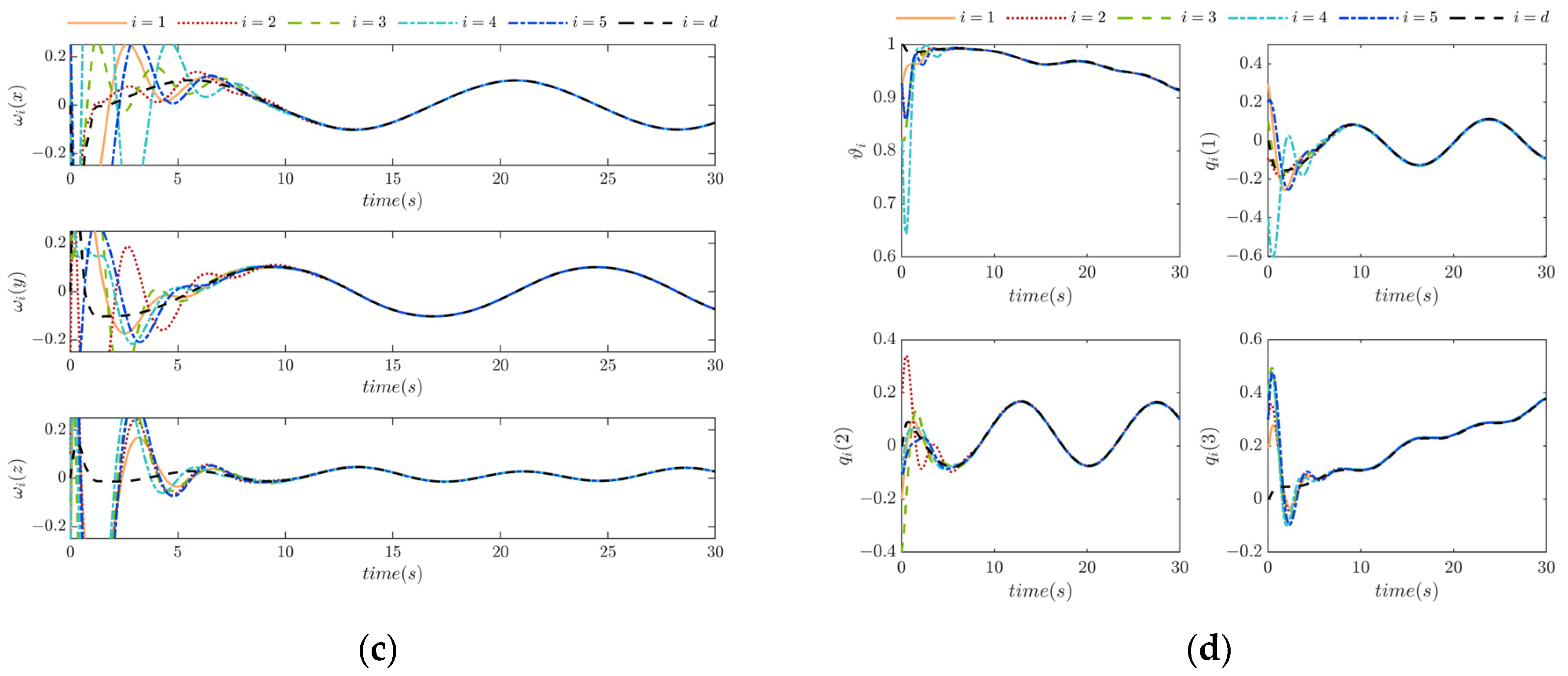
The parameters of the ACSL are set as $k_{p,i}=100$, $k_{p,ij}=15$, and ${\lambda }_i=20$. Then, the parameters for TSM are set as $k_s=2.6$, $r=0.8$, $\lambda =0.006$, and $\mu =250$ for the adaptive law. For the FTFCP, the parameters are predefined as $k_i^1=6$, $k_i^2=6$, $h_p=9$, and $h_q=13$. In Scenario 1, the attitude-tracking results by the ACSL are plotted in Figure 1.

It can be deduced from Figure 1 that the tracking error is suppressed into low levels in less than 8 s, and the errors in the auxiliary system converge rapidly, which can fulfill the attitude control objectives. Furthermore, the initial quaternion and angular rate can be set to a non-zero value, which indicates that the ACSL is not sensitive to the initial state values, and this property exceeds many attitude-tracking laws provided in other studies.

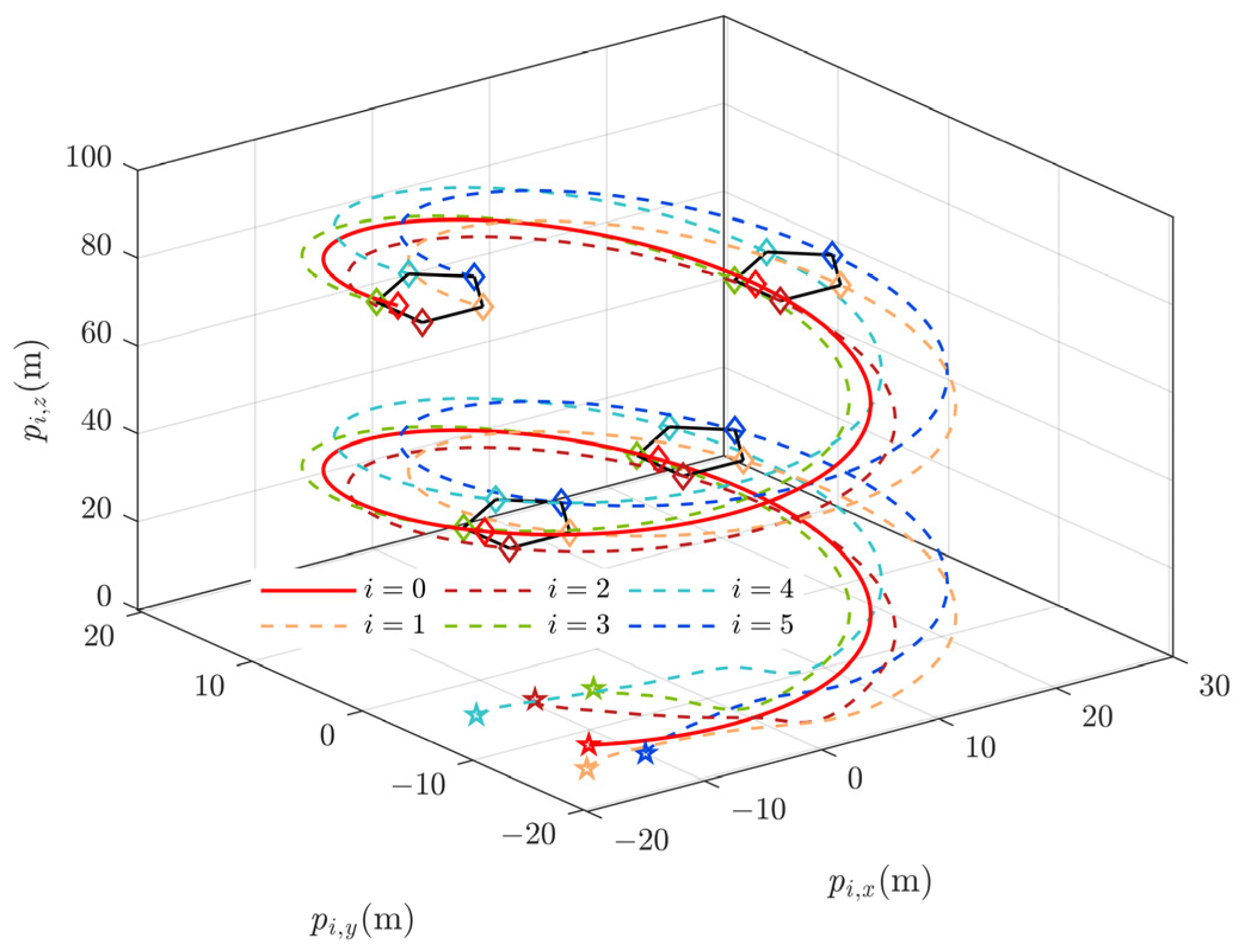
The 3D formation-tracking result is plotted in Figure 2, and the TSM curves and tracking errors of position and velocity are shown in Figure 3.

According to Figure 2 and Figure 3, formation consensus tracking can be achieved in less than 4 s, and the formation control errors in position and velocity are both suppressed to a lower level and converge to zero, just as the analysis in Theorem 2.

Scenario 2: The purpose is to validate the effectiveness of the collision-free control framework including the ACSL, FTFCP, and PHOAP. The reference trajectory is set as the same in Scenario 1. Additionally, the obstacle collision avoidance control law denoted by (20)–(22) is introduced to adjust the motion of the leader UAV. Collision-free control is employed in each follower UAV according to (18), (19), and (23)–(26). Two static obstacles are set to block the desired trajectory at $o_1={\left[9.4447,14.1350,25.5000\right]}^T \mathrm{m}$ with $R_1^o=6.0 \mathrm{m}$, and $o_2={\left[-14.1350,9.4447,46.5000\right]}^T \mathrm{m}$ with $R_2^o=4.0 \mathrm{m}$. The control parameters in the collision-free protocol are set as $K_u^p=\mathrm{diag}\left\{4.0,4.0,4.0\right\}$, $K_u^v=\mathrm{diag}\left\{2.0,2.0,2.0\right\}$, $K_l^o=1.5$, $K_i^o=1.5$, $K_i^c=0.2$, $R^d=8.0$, and $R^s=6.0$. 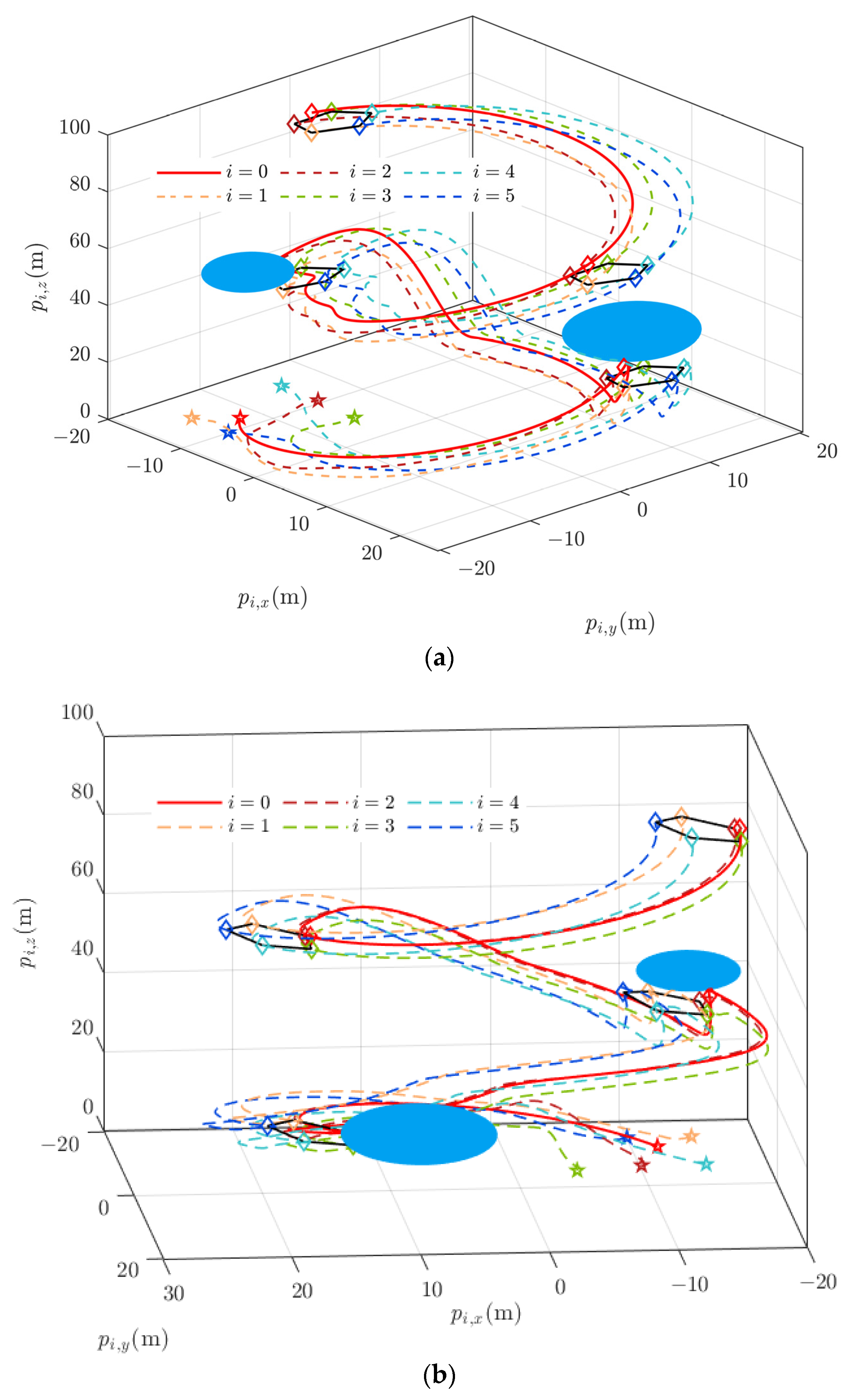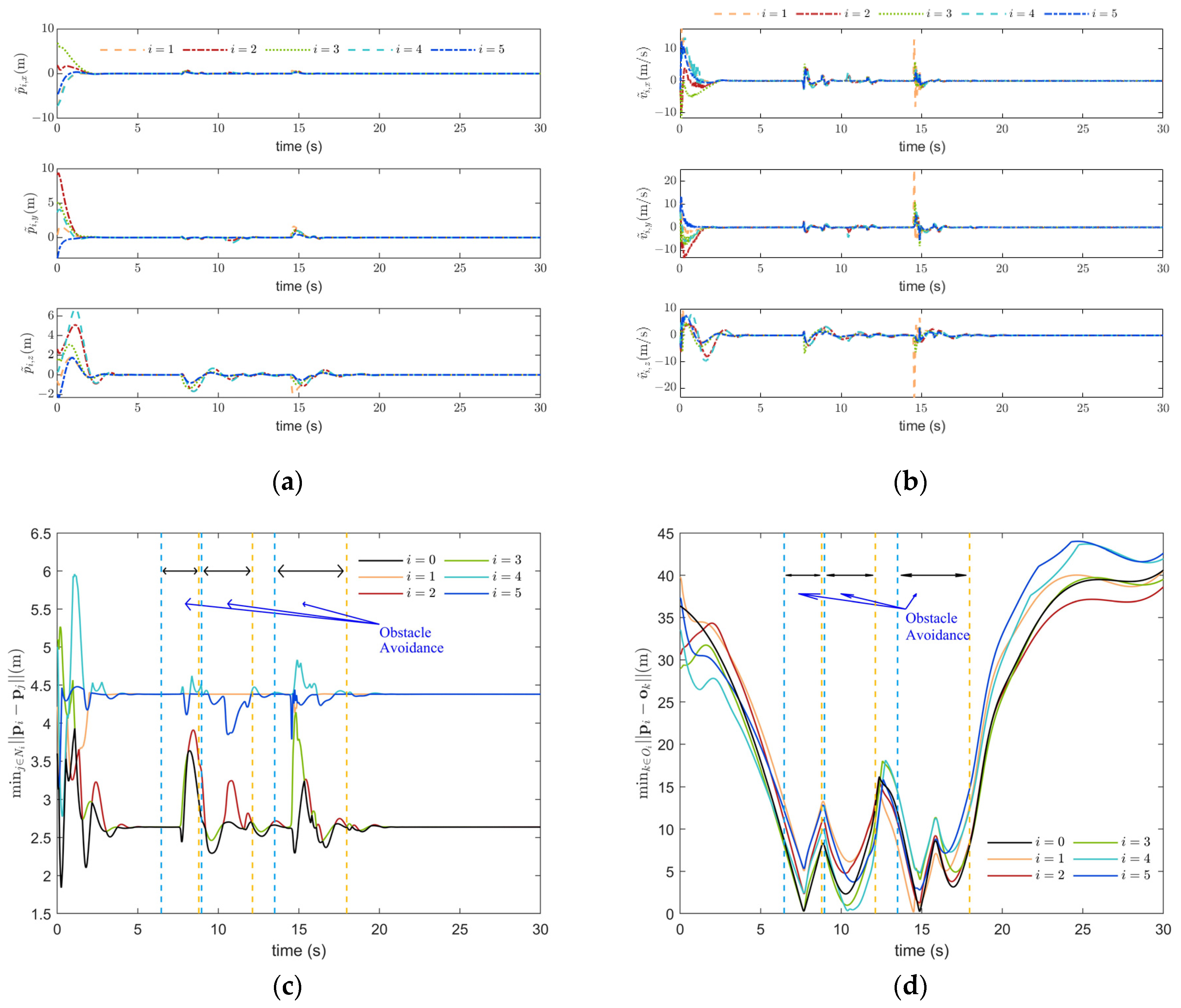The control results are shown in Figure 4 and Figure 5.

It can be deduced from Figure 4 that the UAV formations can evade the existing obstacles, which are blocking the desired path. After avoiding the obstacles, the follower UAVs can rapidly complete the formation pattern reconfiguration around the maneuvering leader target. The relative distance is displayed, which intuitively displays the obstacle evasion and the collision avoidance results in Scenario 2. The proposed methodology is verified to be superior in collision-free control, formation consensus tracking, and formation reconfiguration.

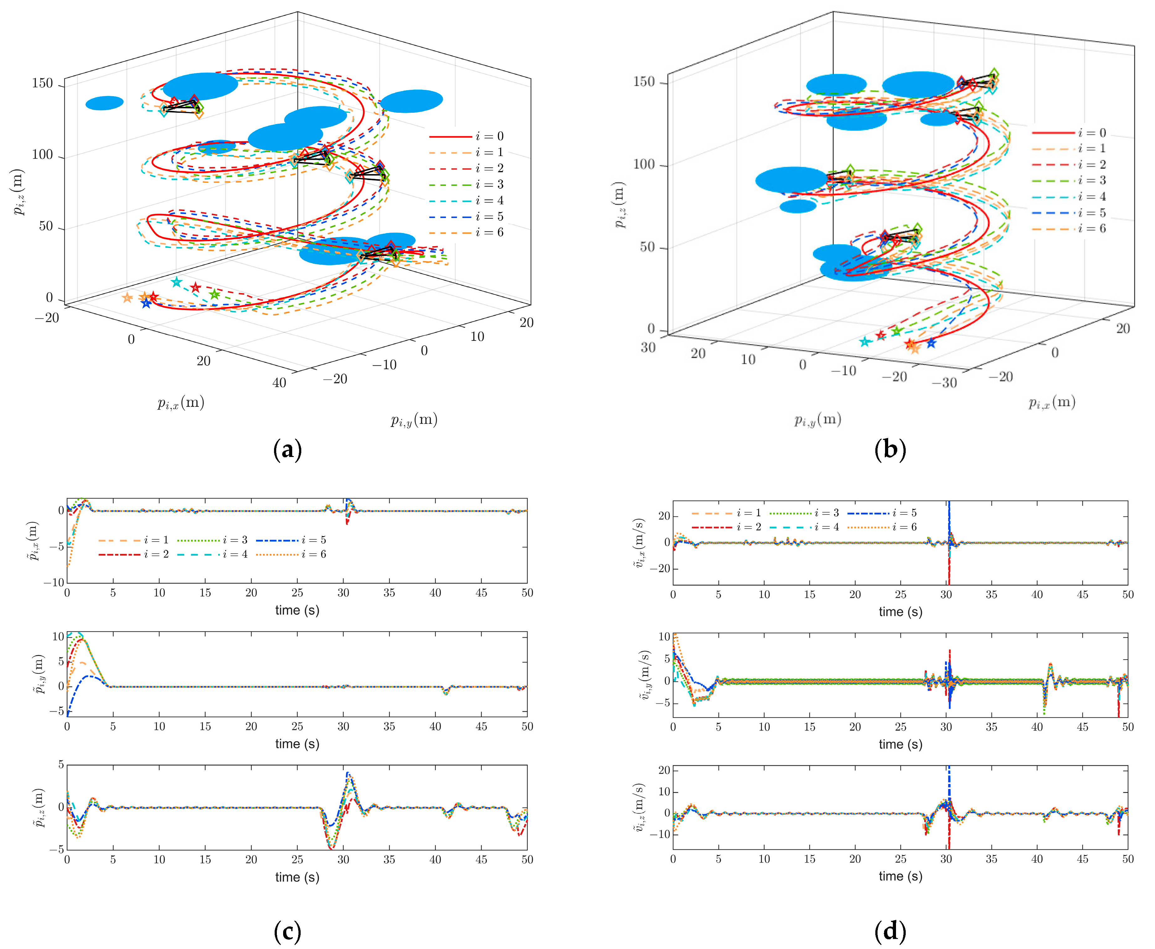
Scenario 3: Another simulation with more obstacles distributed along the predefined trajectories of the UAV cluster is conducted, where the follower UAVs are governed by a completely different formation configuration. In this scenario, one leader node and six follower nodes are considered a leader–follower UAV cluster, defining an interactive topology of $b_{10}=b_{50}=1$ and $b_{20}=b_{30}=b_{40}=b_{60}=0$, and the transmission form between followers are set as an undirected topology with $w_{13}=w_{23}=w_{24}=w_{31}=w_{32}=w_{35}=w_{36}=w_{42}=$$w_{53}=w_{63}=1$. The standard formation configuration without considering the obstacles are indicated as

$${\delta }_i=\left\{\begin{array}{l}{\left[3+5\sqrt{2}\cos \left(-2\pi i/3\right)/2,5\sqrt{2}\sin \left(-2\pi i/3\right)/2,\left|2\cos \left(2\pi i/3\right)\right|\right]}^T \mathrm{m}, i=1,2,3\\ {\left[3+5\sqrt{2}\cos \left(-2\pi \left(i-3\right)/3\right)/2,5\sqrt{2}\sin \left(-2\pi \left(i-3\right)/3\right)/2,-\left|2\cos \left(2\pi \left(i-3\right)/3\right)\right|\right]}^T \mathrm{m}, i=4,5,6\end{array}\right.$$

(46)

Furthermore, the obstacles are set to locate at

$$\begin{array}{l}{o}_1={\left[6.9447,10.6350,24.0000\right]}^T \mathrm{m},R_1^o=6.0 \mathrm{m}, o_2={\left[11.9447,17.6350,27.0000\right]}^T \mathrm{m},R_2^o=4.0 \mathrm{m}\\ o_3={\left[-18.6350,5.9447,82.0000\right]}^T \mathrm{m},R_3^o=3.0 \mathrm{m},o_4={\left[-9.6350,12.9447,89.0000\right]}^T \mathrm{m},R_4^o=6.0 \mathrm{m}\\ o_5={\left[3.9447,8.6350,117.0000\right]}^T \mathrm{m},R_5^o=5.0 \mathrm{m},o_6={\left[14.9447,19.6350,126.0000\right]}^T \mathrm{m},R_6^o=5.0 \mathrm{m}\\ o_7={\left[-14.9447,-19.6350,141.0000\right]}^T \mathrm{m},R_7^o=3.0 \mathrm{m},o_8={\left[-3.9447,-8.6350,150.0000\right]}^T \mathrm{m},R_8^o=6.0 \mathrm{m}\end{array}$$

(47)

The simulation is conducted in anticipation of a formation pattern according to (46) and an obstacle distribution according to (47). Then, the reference trajectory of the leader UAV is set to be the same as in Scenario 1. To display the simulation results, the three-dimensional collision-free formation trajectories are illustrated in subplots (a) and (b) in Figure 6, and the tracking errors of position and velocity are shown by the latter two subplots in Figure 6, respectively.

It can be determined from Figure 5 that collision-free reconfiguration formation control can be maintained among complex obstacles, and the robustness and stability hold for different formation patterns.

To sum up the methodology design and the simulation results of both formation and obstacle avoidance reconfiguration control, the research conducted in this paper has several superior points indicated as follows. Firstly, unlike [27,32,43,44,45], the initial attitude states in this paper can be set as arbitrary values and are finally regulated to the desired value. Moreover, there is no requirement of the direct state feedback of the quaternion, angular velocity, and rotation matrix when implementing auxiliary error systems in this paper. Secondly, a pigeon-hierarchy-inspired collision-free protocol based on potential field gradients is proposed. Unlike [13,14,15,16], the leader–follower structure is considered in formation obstacle avoidance, and the leader’s trajectory is predefined and only adjusted by the virtual potential repulsive force, which maintains the computational efficiency compared with collision avoidance via optimization or random search methodology. Finally, finite-time convergence can be guaranteed in the position loop control, which exceeds those studies that only remain asymptotically stable. Moreover, the adaptive updating law and terminal sliding mode are employed to facilitate the convergence speed and the robustness of reconfiguration.

5. Conclusions

This paper investigates the cooperative formation-tracking framework considering obstacle avoidance for multiple unmanned aerial vehicles. Aiming at attaining consensus tracking in the attitude loop, an attitude consensus stabilization law is established. The high-precision pose measurement from expensive airborne sensors is abandoned by introducing an auxiliary error system, and the applied torque can be yielded only by attitude control errors instead of the accurate state feedback. Furthermore, an adaptive finite-time formation control protocol is proposed by introducing terminal sliding mode and is proved to reach practical finite-time stability in the translational loop by Lyapunov theories. Additionally, a pigeon-hierarchy-inspired obstacle avoidance approach is established by employing an improved potential field. Collision-free control can be achieved by combining the collision avoidance protocol with the finite-time formation control law, and the collision between quadrotor UAVs or between UAVs and obstacles are controlled in a cascaded interaction sequence from leader to followers. The proposed methodology is validated through numerical simulation.