
GTrXL-SAC-Based Path Planning and Obstacle-Aware Control Decision-Making for UAV Autonomous Control

 , , ,
, , ,  ,
,
Abstract
1. Introduction
2. Related Work
- Challenges in UAV Modeling
- Long-Term Dependency Problem in DRL
3. Theoretical Foundations and Core Principles
3.1. AirSim Simulation Environment
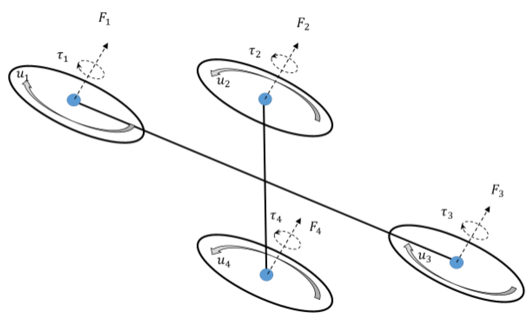
3.2. Quadrotor UAV Model
- Kinematic Model of the UAV
- Dynamic Model of the UAV
3.3. Soft Actor-Critic (SAC) Algorithm in Reinforcement Learning
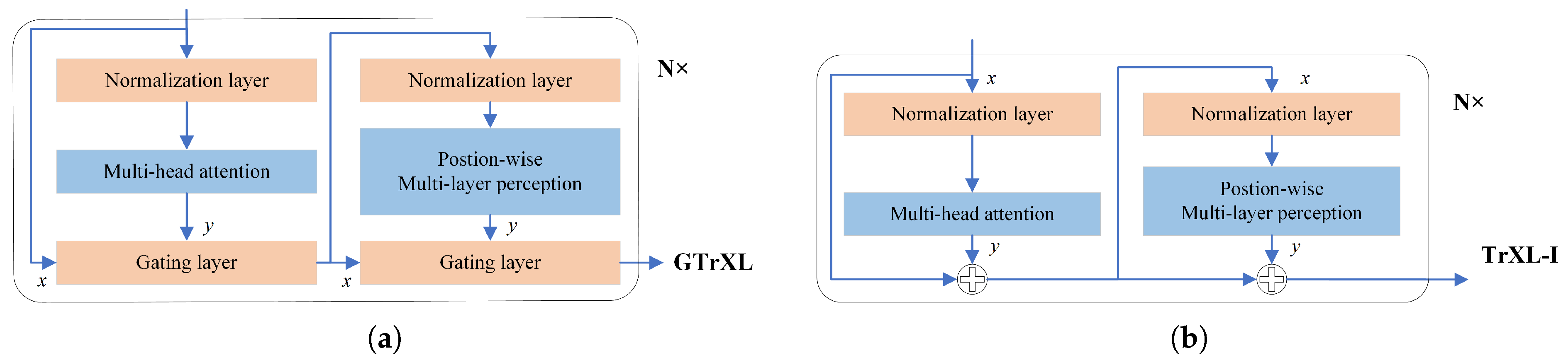
3.4. Attention Mechanism: Gated Transformer-XL (GTrXL) Architecture
- Identity Map Reordering
- Relative Positional Encoding
- The Gating Layer
4. UAV Control Based on the GTrXL-SAC Algorithm
4.1. Mathematical Modeling of Decision Problems
4.1.1. Problem Formulation
- State Space
- Action Space
4.1.2. Long-Term Dependency Modeling in Sequential Decision Processes
4.1.3. Objective Function and Operational Constraints
- Objective Function
- Reward Function and Operational Constraints
4.2. The Algorithm Flow
- Phase 1
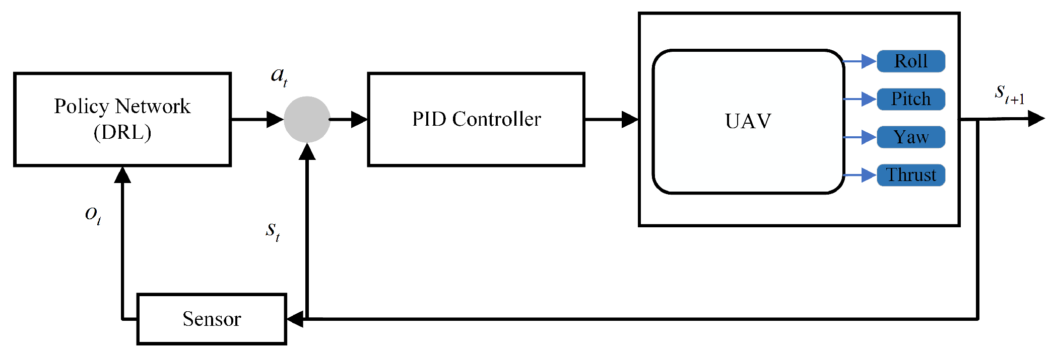
- Perception and Decision-Making Phase
- Phase 1-1
- Initialize the parameters of the policy network (Actor) parameters , the Q-network (Critic) parameters , and the target Q-network parameters . Both the actor and critic networks incorporate GTrXL. If the state information includes images, a CNN is used within the network to process the image data.
- Phase 1-2
- The sensor information is embedded and encoded in terms of relative position to represent the current input state:where represents the current input state.
- Phase 1-3
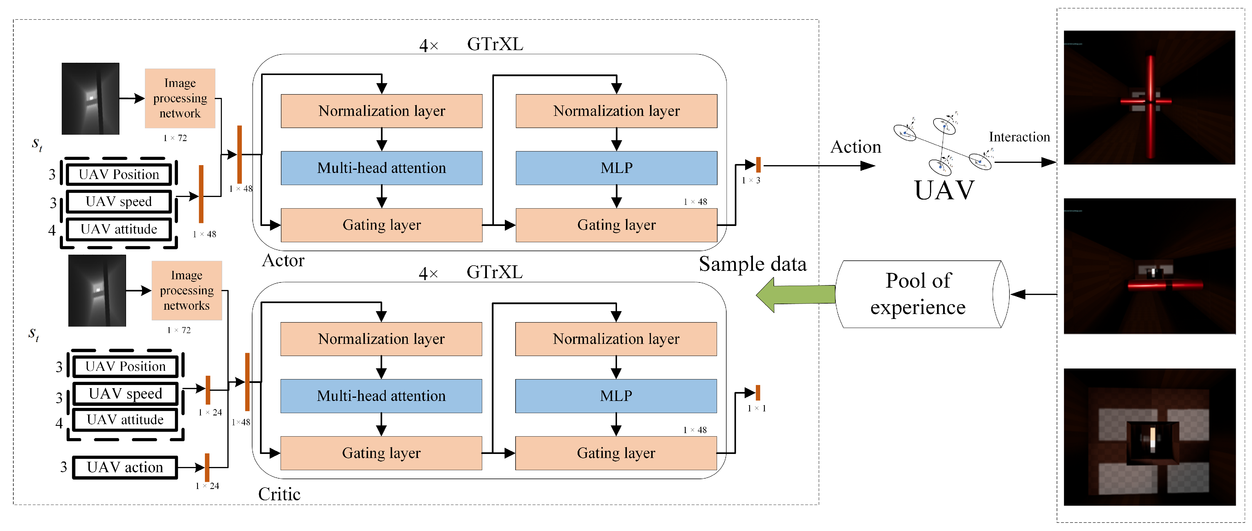
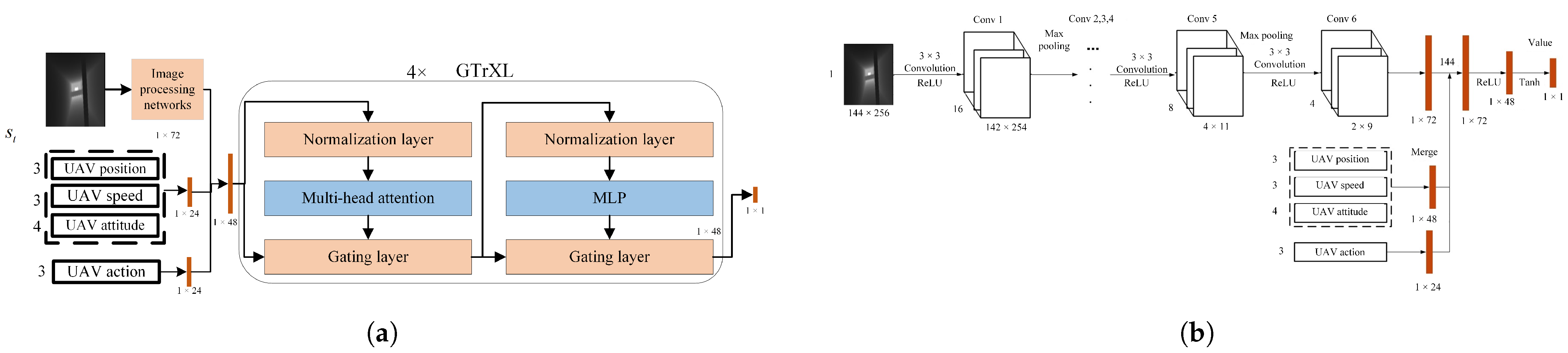
- After receiving the input embedding, GTrXL computes the UAV’s action .As shown in Figure 4, the internal operation flow of GTrXL for obtaining the action is as follows:
- Acquire Memory Information;
- Merge Memory Information with Current Input Embedding : ;
- Perform Normalization;
- The attention distribution is computed according to the equation ;
- The attention distribution and positional encoding (PE) are processed through a gating mechanism (GRU1) to obtain the result , with the internal computation described by Equation (20);
- Perform normalization;
- The multilayer perceptron (MLP) computation: Here, the MLP essentially refers to a fully connected neural network;
- The result and the output of the multilayer perceptron are processed through a gating mechanism (GRU2) to obtain the final output o;
- The output is passed through a softmax function to obtain the UAV’s action .
- Phase 1-4
- Update the memory information.
| Algorithm 1 Pseudocode for the GTrXL-SAC algorithm. |
| Input: Initialize an empty experience pool, entropy regularization coefficient, maximum simulation steps per round T, step size start_size for starting with the policy network, and batch size batch_size for training. |
| Output: UAV flight strategy. |
| 1. Initialize the strategy network weights , Q network weights , and target Q network weights . |
| 2. For episode = 0, 1, …, n: |
| 3. Reset the environment and obtain the initial state . |
| 4. While the task is not completed: |
| 5. t < start_size: |
| 6. . |
| 7. ELSE |
| 8. The Actor network outputs an action ; |
| 9. The UAV executes an action , obtains the next state , and calculates the reward ; |
| 10. The transition tuple is stored in the experience pool. |
| 11. IF the number of transition tuples stored in the experience pool > batch_size: |
| 12. Based on formula |
| , calculate the loss value of the Q network and compute the gradient with respect to the parameters ; |
| 13. Compute the loss value of the policy network based on Equation , and calculate the gradient of the parameter with respect to the loss; |
| 14. Compute the loss value of the entropy regularization coefficient based on Equation , and calculate the gradient of the parameter . |
| 15. Update the parameters , of the policy network and Q-network according to optimization algorithms; |
| 16. Update the target Q-network. |
| 17. End IF |
| 18. Jump to step 5. |
| 19. End For |
5. Network Architecture and Parameter Design
5.1. Network Architecture Design
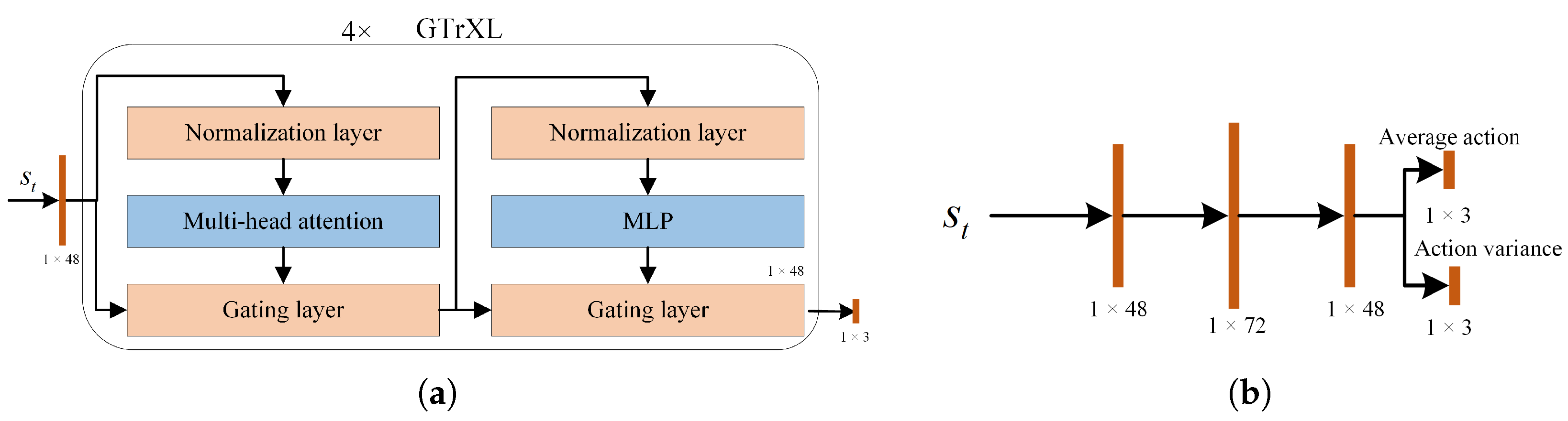
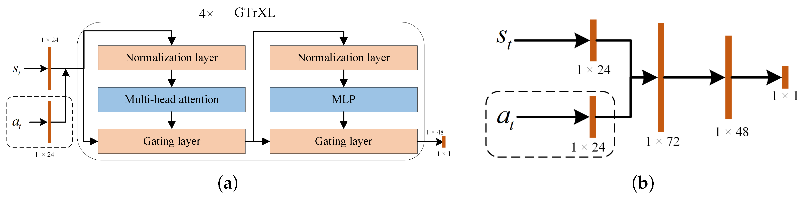
5.1.1. Actor–Critic Architecture Based on Sensor Data
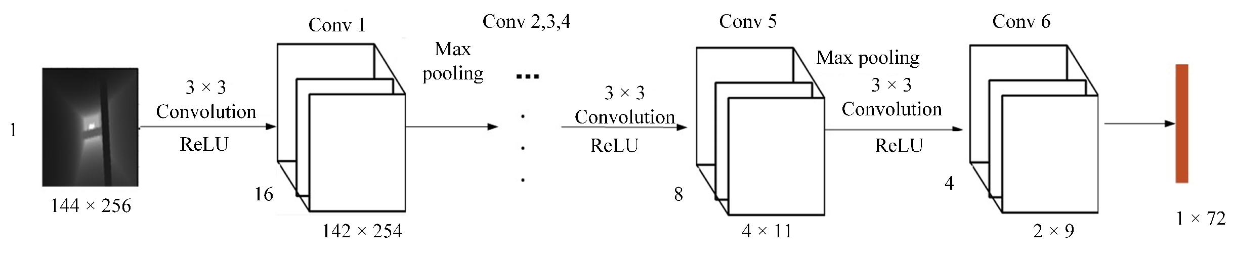
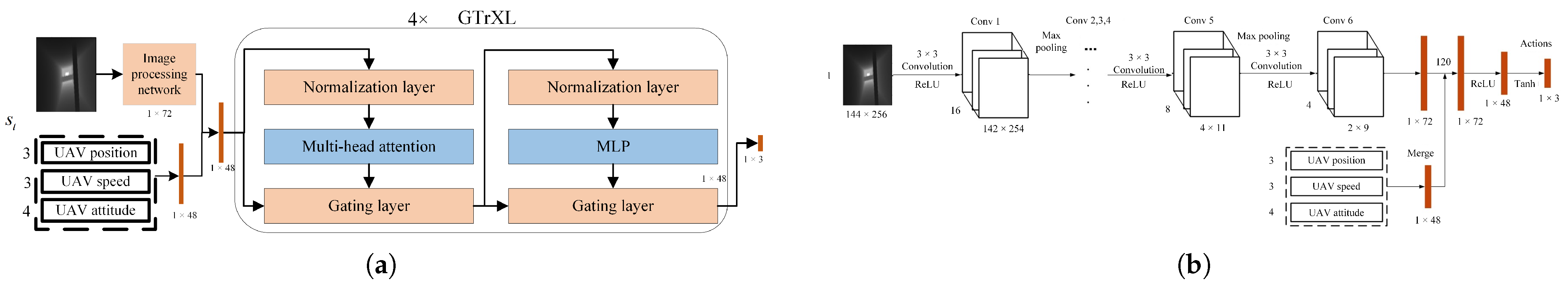
5.1.2. Actor–Critic Architecture Based on Multimodal Data
5.2. Algorithm Parameter Design
6. Experimental Design and Results Analysis with Discussion
6.1. Simulation Environment Design
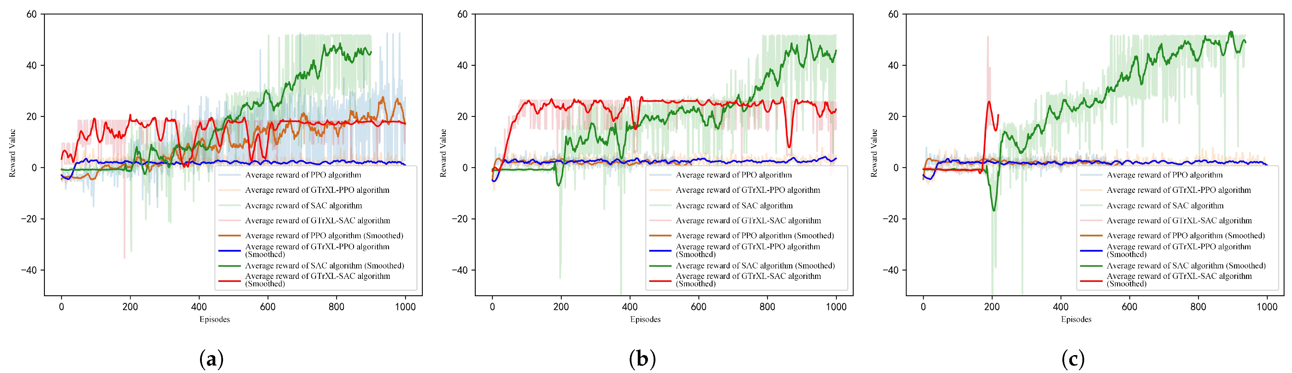
6.2. Experiment 1: UAV Perception and Control with Sensor Data as Input
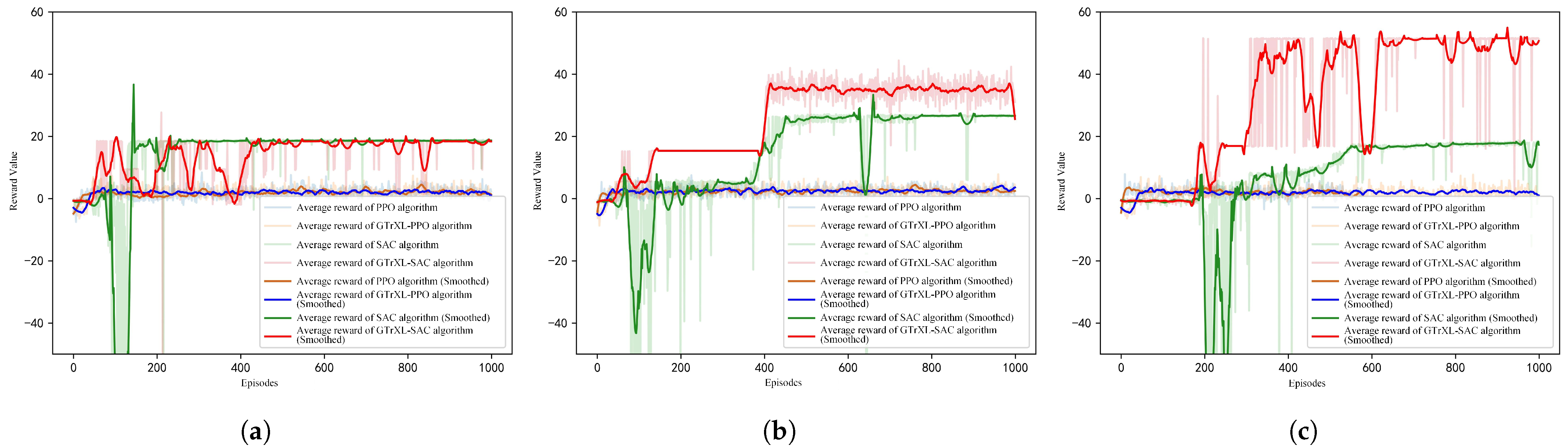
- Training Speed Comparison
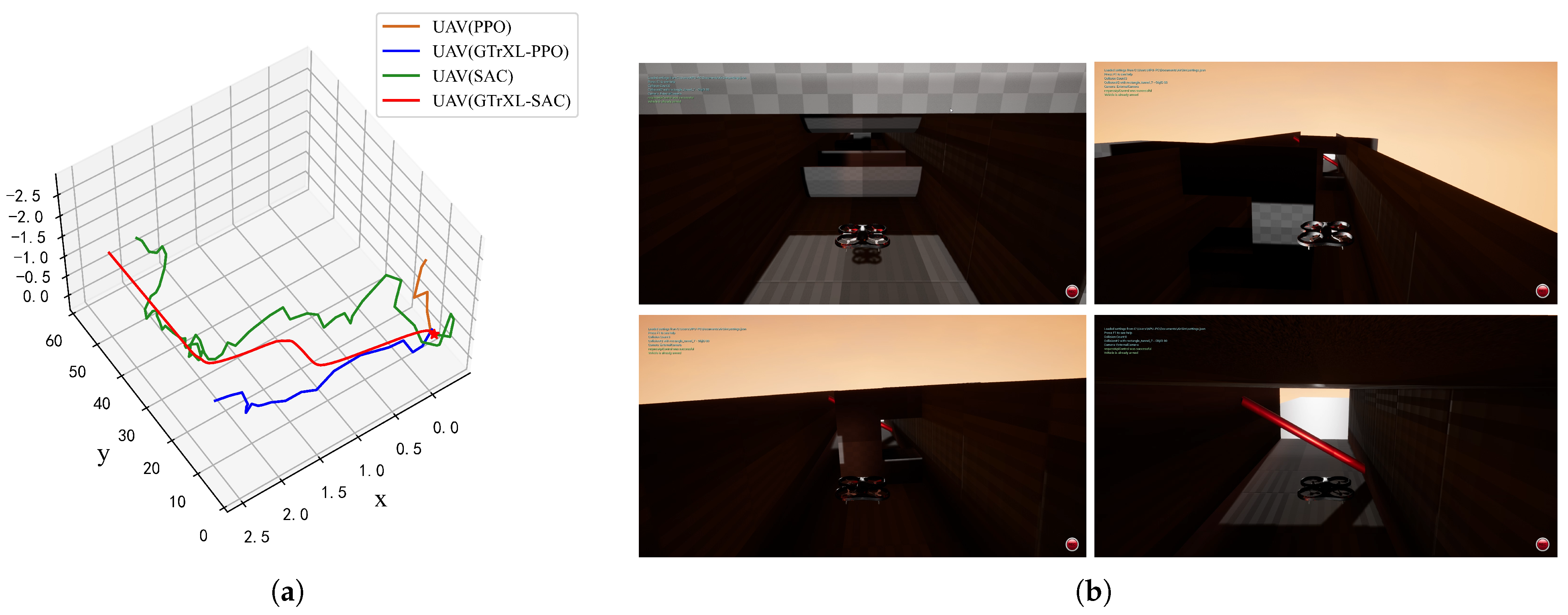
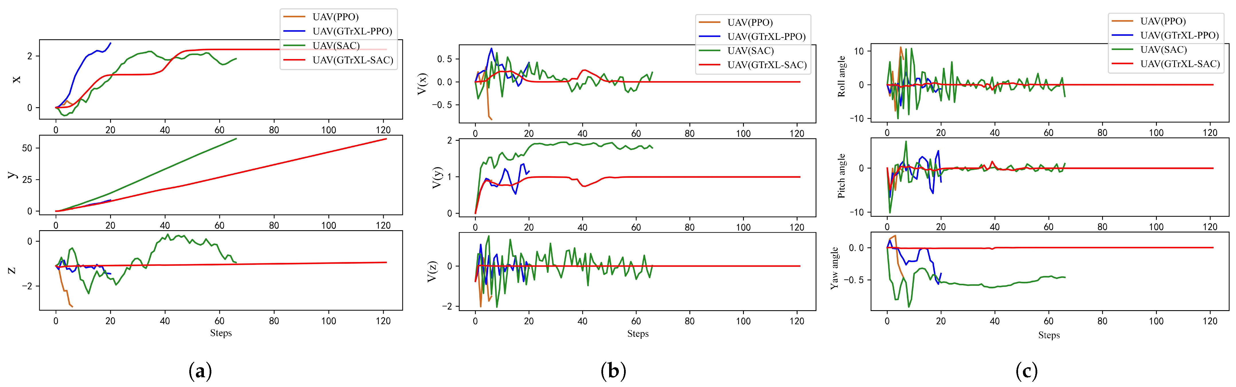
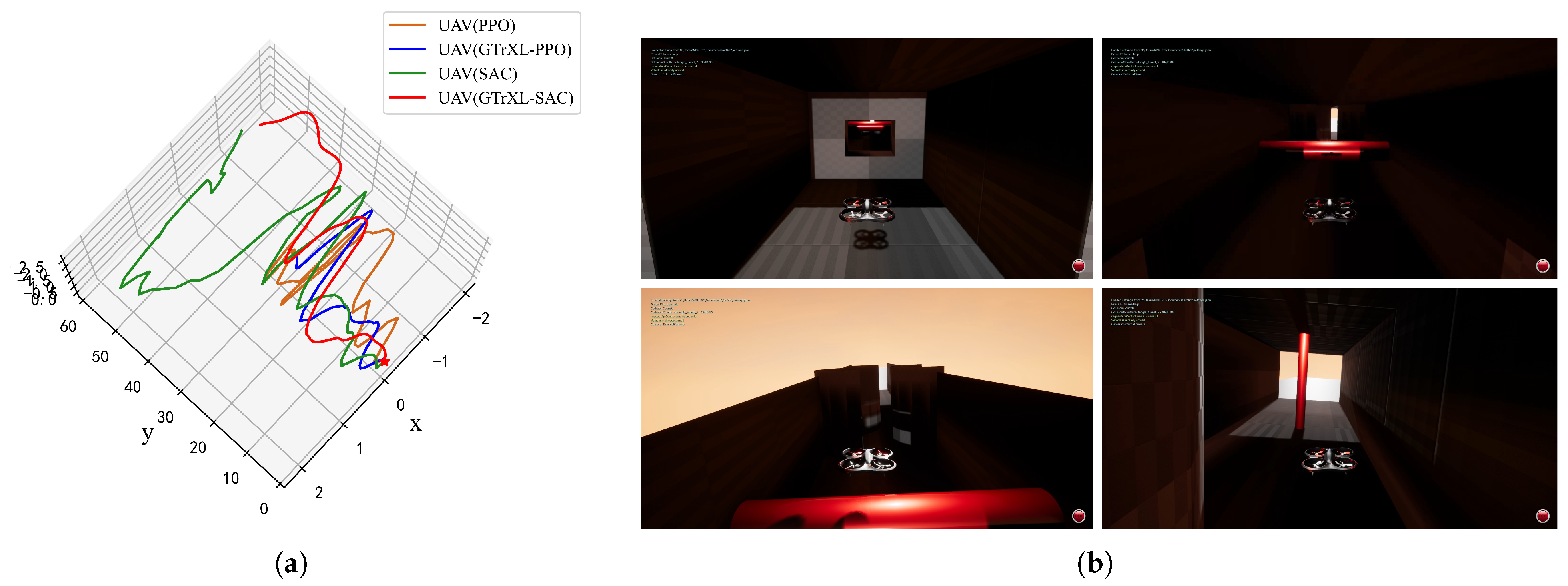
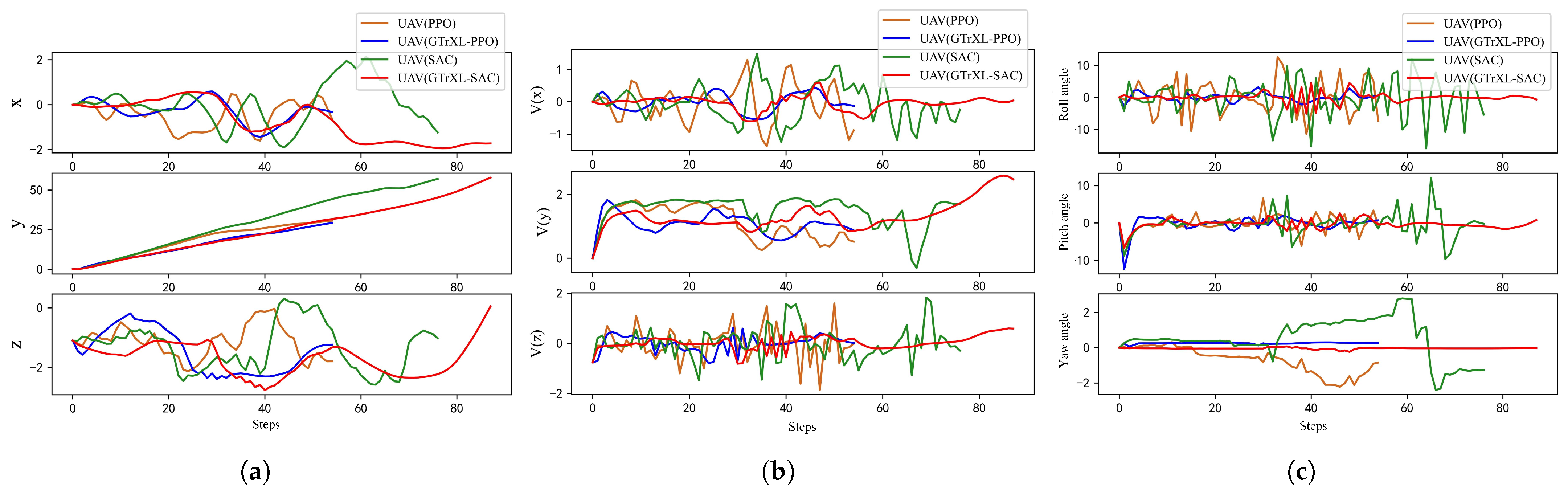
- Comparison of Testing Results
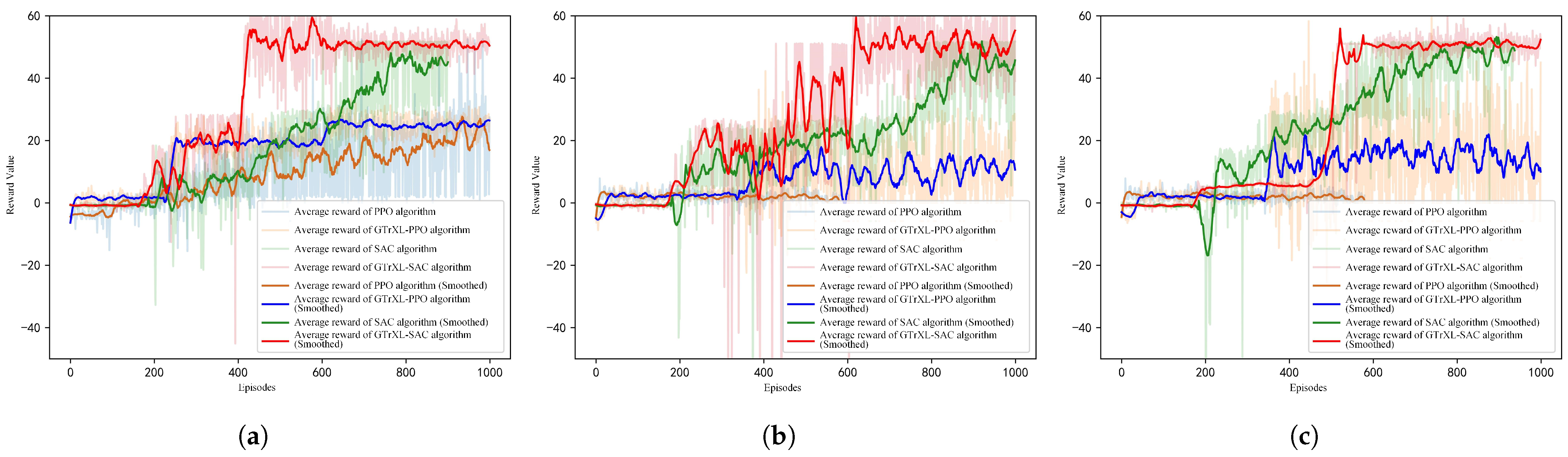
6.3. Experiment 2: UAV Perception and Control with Multimodal Data as Input
- Comparison of Training Speeds
- Comparison of Testing Results
7. Conclusions and Future Work
Author Contributions
Funding
Data Availability Statement
Acknowledgments
Conflicts of Interest
References
- Federal Aviation Administration; U.S. Department of Transportation. FAA Aerospace Forecast: Fiscal Years 2024–2044. 2024. Available online: https://www.faa.gov (accessed on 2 November 2024).
- Gohari, A.; Ahmad, A.B.; Rahim, R.B.A.; Supa’at, A.S.M.; Razak, S.A.; Gismalla, M.S.M. Involvement of Surveillance Drones in Smart Cities: A Systematic Review. IEEE Access 2022, 10, 56611–56628. [Google Scholar] [CrossRef]
- Zhang, C.; Kovacs, J.M. The application of small unmanned aerial systems for precision agriculture: A review. Precision Agric. 2012, 13, 693–712. [Google Scholar]
- Osorio Quero, C.; Martinez-Carranza, J. Unmanned aerial systems in search and rescue: A global perspective on current challenges and future applications. Int. J. Disaster Risk Reduct. 2025, 118, 105199. [Google Scholar] [CrossRef]
- Xiao, Z.W.; Fu, X.W. A Cooperative Detection Game: UAV Swarm vs. One Fast Intruder. J. Syst. Eng. Electron. 2023, 34, 1565–1575. [Google Scholar]
- Li, B.; Wang, J.; Song, C.; Yang, Z.; Wan, K.; Zhang, Q. Multi-UAV roundup strategy method based on deep reinforcement learning CEL-MADDPG algorithm. Expert Syst. Appl. 2024, 245, 123018. [Google Scholar] [CrossRef]
- Xu, Q.; Yi, J.; Wang, X.; Niu, M.-B.; Miah, M.S.; Wang, L. Secure Unmanned Aerial Vehicle Communication in Dual-Function Radar Communication System by Exploiting Constructive Interference. Drones 2024, 8, 581. [Google Scholar] [CrossRef]
- AlMahamid, F.; Grolinger, K. Autonomous Unmanned Aerial Vehicle navigation using Reinforcement Learning: A systematic review. Eng. Appl. Artif. Intell. 2022, 115, 105321. [Google Scholar]
- Wu, J.H.; Ye, Y.; Du, J. Multi-objective reinforcement learning for autonomous drone navigation in urban areas with wind zones. Autom. Constr. 2024, 158, 105253. [Google Scholar]
- Fu, X.W.; Zhu, J.D.; Wei, Z.Y.; Wang, H.; Li, S.L. A UAV Pursuit-Evasion Strategy Based on DDPG and Imitation Learning. Int. J. Aerosp. Eng. 2022, 2022, 3139610. [Google Scholar]
- Russell, S.J.; Norvig, P. Artificial Intelligence: A Modern Approach, 4th ed.; Pearson: London, UK, 2020. [Google Scholar]
- Chalapathy, R.; Chawla, S. Deep Learning for Anomaly Detection: A Survey. arXiv 2019, arXiv:1901.03407. [Google Scholar]
- Caballero-Martin, D.; Lopez-Guede, J.M.; Estevez, J.; Graña, M. Artificial Intelligence Applied to Drone Control: A State of the Art. Drones 2024, 8, 296. [Google Scholar] [CrossRef]
- Arulkumaran, K.; Deisenroth, M.P.; Brundage, M.; Bharath, A.A. Deep Reinforcement Learning: A Brief Survey. IEEE Signal Process. Mag. 2017, 34, 26–38. [Google Scholar] [CrossRef]
- Hochreiter, S.; Schmidhuber, J. Long Short-Term Memory. Neural Comput. 1997, 9, 1735–1780. [Google Scholar] [CrossRef] [PubMed]
- Vaswani, A.; Shazeer, N.; Parmar, N.; Uszkoreit, J.; Jones, L.; Gomez, A.N.; Kaiser, L.; Polosukhin, I. Attention Is All You Need. arXiv 2024, arXiv:1706.03762. [Google Scholar]
- Roberge, V.; Tarbouchi, M.; Labonté, G. Fast genetic algorithm path planner for fixed-wing military UAV using GPU. IEEE Trans. Aerosp. Electron. Syst. 2018, 54, 2105–2117. [Google Scholar] [CrossRef]
- Chen, J.; Ye, F.; Jiang, T. Path planning under obstacle-avoidance constraints based on ant colony optimization algorithm. In Proceedings of the 2017 IEEE 17th International Conference on Communication Technology (ICCT), Chengdu, China, 27–30 October 2017; pp. 1434–1438. [Google Scholar]
- Liu, Y.; Zhang, X.; Guan, X.; Delahaye, D. Adaptive sensitivity decision based path planning algorithm for unmanned aerial vehicle with improved particle swarm optimization. Aerosp. Sci. Technol. 2016, 58, 92–102. [Google Scholar] [CrossRef]
- Zhang, X.; Lu, X.; Jia, S.; Li, X.Z. A novel phase angle-encoded fruit fly optimization algorithm with mutation adaptation mechanism applied to UAV path planning. Appl. Soft Comput. 2018, 70, 371–388. [Google Scholar]
- Chen, Y.B.; Mei, Y.S.; Yu, J.Q.; Su, X.L.; Xu, N. Three-dimensional unmanned aerial vehicle path planning using modified wolf pack search algorithm. Neurocomputing 2017, 266, 445–457. [Google Scholar]
- Zhang, D.Q.; Xian, Y.; Li, J.; Lei, G.; Chang, Y. UAV path planning based on chaos ant colony algorithm. In Proceedings of the IEEE 2015 International Conference on Computer Science and Mechanical Automation (CSMA), Hangzhou, China, 23–25 October 2015; pp. 81–85. [Google Scholar]
- Yan, C.; Xiang, X. A path planning algorithm for uav based on improved q-learning. In Proceedings of the IEEE 2018 2nd International Conference on Robotics and Automation Sciences (ICRAS), Wuhan, China, 23–25 June 2018; pp. 1–5. [Google Scholar]
- Menfoukh, K.; Touba, M.M.; KhenfriI, F.; Guettal, L. Optimized Convolutional Neural Network architecture for UAV navigation within unstructured trail. In Proceedings of the IEEE 2020 1st International Conference on Communications, Control Systems and Signal Processing (CCSSP), El Oued, Algeria, 16–17 May 2020; pp. 211–214. [Google Scholar]
- Back, S.; Cho, G.; Oh, J.; Tran, X.T.; Oh, H. Autonomous UAV trail navigation with obstacle avoidance using deep neural networks. J. Intell. Robot. Syst. 2020, 100, 1195–1211. [Google Scholar]
- Maciel-Pearson, B.G.; Carbonneau, P.; Breckon, T.P. Extending deep neural network trail navigation for unmanned aerial vehicle operation within the forest canopy. In Proceedings of the 19th Annual Conference Towards Autonomous Robotic Systems, Bristol, UK, 25–27 July 2018; Springer International Publishing: Cham, Switzerland, 2018; pp. 147–158. [Google Scholar]
- Chhikara, P.; Tekchandani, R.; Kumar, N.; Chamola, V.; Guizani, M. DCNN-GA: A deep neural net architecture for navigation of UAV in indoor environment. IEEE Internet Things J. 2020, 8, 4448–4460. [Google Scholar]
- Doukhi, O.; Lee, D.J. Deep reinforcement learning for autonomous map-less navigation of a flying robot. IEEE Access 2022, 10, 82964–82976. [Google Scholar]
- Bouhamed, O.; Ghazzai, H.; Besbes, H.; Massoud, Y. Autonomous UAV navigation: A DDPG-based deep reinforcement learning approach. In Proceedings of the 2020 IEEE International Symposium on circuits and systems (ISCAS), Sevilla, Spain, 10–21 October 2020; pp. 1–5. [Google Scholar]
- He, L.; Aouf, N.; Whidborne, J.F.; Song, B.F. Deep reinforcement learning based local planner for UAV obstacle avoidance using demonstration data. arXiv 2020, arXiv:2008.02521. [Google Scholar]
- Liu, C.H.; Ma, X.X.; Gao, X.D.; Tang, J. Distributed energy-efficient multi-UAV navigation for long-term communication coverage by deep reinforcement learning. IEEE Trans. Mob. Comput. 2019, 19, 1274–1285. [Google Scholar]
- Mellinger, D.; Kumar, V. Minimum snap trajectory generation and control for quadrotors. In Proceedings of the 2011 IEEE International Conference on Robotics and Automation, Shanghai, China, 9–13 May 2011; pp. 2520–2525. [Google Scholar] [CrossRef]
- Daniel, M. Trajectory Generation and Control for Quadrotors; University of Pennsylvania: Philadelphia, PA, USA, 2012. [Google Scholar]
- Zhang, Y.J.; Huang, Y.J.; Liang, K.; Cao, K.; Wang, Y.F.; Liu, X.C.; Guo, Y.Z.; Wang, J.Z. High-precision modeling and collision simulation of small rotor UAV. Aerosp. Sci. Technol. 2021, 118, 106977. [Google Scholar]
- Deverett, B.; Faulkner, R.; Fortunato, M.; Wayne, G.; Leibo, J.Z. Interval timing in deep reinforcement learning agents. arXiv 2024, arXiv:1905.13469. [Google Scholar]
- Schrittwieser, J.L.; Antonoglou, I.; Hubert, T.; Simonyan, K.; Sifre, L.; Schmitt, S.; Guez, A.; Lockhart, E.; Hassabis, D.; Graepel, T.; et al. Mastering Atari, Go, Chess and Shogi by Planning with a Learned Model. arXiv 2024, arXiv:1911.08265. [Google Scholar]
- Gupta, S.; Singal, G.; Garg, D. Deep Reinforcement Learning Techniques in Diversified Domains: A Survey. Arch. Computat. Methods Eng. 2021, 28, 4715–4754. [Google Scholar] [CrossRef]
- Mienye, I.D.; Swart, T.G.; Obaido, G. Recurrent Neural Networks: A Comprehensive Review of Architectures, Variants, and Applications. Information 2024, 15, 517. [Google Scholar] [CrossRef]
- Shital, S.; Dey, D.; Chris, L.; Ashish, K. AirSim: High-Fidelity Visual and Physical Simulation for Autonomous Vehicles. arXiv 2017, arXiv:1705.05065. [Google Scholar]
- Tuomas, H.; Aurick, Z.; Pieter, A.; Sergey, L. Soft Actor-Critic: Off-Policy Maximum Entropy Deep Reinforcement Learning with a Stochastic Actor. arXiv 2018, arXiv:1801.01290. [Google Scholar]
- Tuomas, H.; Aurick, Z.; Kristian, H.; George, T.; Sehoon, H.; Jie, T.; Vikash, K.; Henry, Z.; Abhishek, G.; Pieter, A.; et al. Soft Actor-Critic Algorithms and Applications. arXiv 2018, arXiv:1812.05905. [Google Scholar]
- Parisotto, E.; Song, H.F.; Rae, J.W.; Pascanu, R.; Gulcehre, C.; Jayakumar, S.M.; Jaderberg, M.; Kaufman, R.L.; Clark, A.; Noury, S.; et al. Stabilizing Transformers for Reinforcement Learning. arXiv 2020, arXiv:1910.06764. [Google Scholar]


| Neural Network Name | Convolutional Kernel Parameters/ Input and Output Dimensions | Activation Function |
|---|---|---|
| Convolutional Layer-1 | Convolutional Kernel: 3 × 3 × 16 Stride: 1 | ELU |
| Pooling Layer-1 | Convolutional Kernel: 4 × 4 Stride: 2 | - |
| Convolutional Layer-2 | Convolutional Kernel: 3 × 3 × 32 Stride: 1 | ELU |
| Pooling Layer-2 | Convolutional Kernel: 4 × 4 Stride: 2 | - |
| Convolutional Layer-3 | Convolutional Kernel: 3 × 3 × 32 Stride: 1 | ELU |
| Pooling Layer-3 | Convolutional Kernel: 3 × 3 Stride: 2 | - |
| Convolutional Layer-4 | Convolutional Kernel: 3 × 3 × 16 Stride: 1 | ELU |
| Pooling Layer-4 | Convolutional Kernel: 3 × 3 Stride: 2 | - |
| Convolutional Layer-5 | Convolutional Kernel: 3 × 3 × 8 Stride: 1 | ELU |
| Convolutional Layer-6 | Convolutional Kernel: 3 × 3 × 4 Stride: 1 | ELU |
| Fully Connected Layer-1 | Input and Output Dimensions: (10, 48) | Tanh |
| Fully Connected Layer-2 | Input and Output Dimensions: (120, 48) | Tanh |
| GTrXL-1 | Input and Output Dimensions: (48, 48) | - |
| GTrXL-2 | Input and Output Dimensions: (48, 48) | - |
| GTrXL-3 | Input and Output Dimensions: (48, 48) | - |
| GTrXL-4 | Input and Output Dimensions: (48, 48) | - |
| Fully Connected Layer-3 | Input and Output Dimensions: (48, 3) | Softmax |
| Neural Network Name | Convolutional Kernel Parameters/ Input and Output Dimensions | Activation Function |
|---|---|---|
| Convolutional Layer-1 | Convolutional Kernel: 3 × 3 × 16 Stride: 1 | ELU |
| Pooling Layer-1 | Convolutional Kernel: 4 × 4 Stride: 2 | - |
| Convolutional Layer-2 | Convolutional Kernel: 3 × 3 × 32 Stride: 1 | ELU |
| Pooling Layer-2 | Convolutional Kernel: 4 × 4 Stride: 2 | - |
| Convolutional Layer-3 | Convolutional Kernel: 3 × 3 × 32 Stride: 1 | ELU |
| Pooling Layer-3 | Convolutional Kernel: 3 × 3 Stride: 2 - | - |
| Convolutional Layer-4 | Convolutional Kernel: 3 × 3 × 16 Stride: 1 | ELU |
| Pooling Layer-4 | Convolutional Kernel: 3 × 3 Stride: 2 | - |
| Convolutional Layer-5 | Convolutional Kernel: 3 × 3 × 8 Stride: 1 | ELU |
| Convolutional Layer-6 | Convolutional Kernel: 3 × 3 × 4 Stride: 1 | ELU |
| Fully Connected Layer-1 | Input and Output Dimensions: (10, 24) | Tanh |
| Fully Connected Layer-2 | Input and Output Dimensions: (10, 24) | Tanh |
| Fully Connected Layer-3 | Input and Output Dimensions: (120, 48) | Tanh |
| GTrXL-1 | Input and Output Dimensions: (48, 48) | - |
| GTrXL-2 | Input and Output Dimensions: (48, 48) | - |
| GTrXL-3 | Input and Output Dimensions: (48, 48) | - |
| GTrXL-4 | Input and Output Dimensions: (48, 48) | - |
| Fully Connected Layer-4 | Input and Output Dimensions: (48, 1) | Softmax |
| Parameters | Values | Parameters | Values |
|---|---|---|---|
| lr | 0.0004 | batch_size | 256 |
| 0.2 | Maximum episodes | 1000 | |
| EPS | Maximum steps per episode | 200 | |
| 0.995 | Loss_coeff_value | 0.5 | |
| 0.97 | Loss_coeff_entropy | 0.01 | |
| Number of sampling episodes | 10 |
| Parameters | Values |
|---|---|
| Entropy regularization coefficient | Initialized to 0.2 with automatic decay |
| lr | 0.0006 |
| Experience replay buffer size | 100,000 |
| batch_size | 256 |
| Exploration noise | 0.1 |
| Target network update frequency | 1 |
| Training start steps | 1000 |
Disclaimer/Publisher’s Note: The statements, opinions and data contained in all publications are solely those of the individual author(s) and contributor(s) and not of MDPI and/or the editor(s). MDPI and/or the editor(s) disclaim responsibility for any injury to people or property resulting from any ideas, methods, instructions or products referred to in the content. |
© 2025 by the authors. Licensee MDPI, Basel, Switzerland. This article is an open access article distributed under the terms and conditions of the Creative Commons Attribution (CC BY) license (https://creativecommons.org/licenses/by/4.0/).
Share and Cite
Huang, J.; Cui, Y.; Xi, G.; Bai, S.; Li, B.; Wang, G.; Neretin, E. GTrXL-SAC-Based Path Planning and Obstacle-Aware Control Decision-Making for UAV Autonomous Control. Drones 2025, 9, 275. https://doi.org/10.3390/drones9040275
Huang J, Cui Y, Xi G, Bai S, Li B, Wang G, Neretin E. GTrXL-SAC-Based Path Planning and Obstacle-Aware Control Decision-Making for UAV Autonomous Control. Drones. 2025; 9(4):275. https://doi.org/10.3390/drones9040275
Chicago/Turabian StyleHuang, Jingyi, Yujie Cui, Guipeng Xi, Shuangxia Bai, Bo Li, Geng Wang, and Evgeny Neretin. 2025. "GTrXL-SAC-Based Path Planning and Obstacle-Aware Control Decision-Making for UAV Autonomous Control" Drones 9, no. 4: 275. https://doi.org/10.3390/drones9040275
APA StyleHuang, J., Cui, Y., Xi, G., Bai, S., Li, B., Wang, G., & Neretin, E. (2025). GTrXL-SAC-Based Path Planning and Obstacle-Aware Control Decision-Making for UAV Autonomous Control. Drones, 9(4), 275. https://doi.org/10.3390/drones9040275