Article

Inversion Model for Total Nitrogen in Rhizosphere Soil of Silage Corn Based on UAV Multispectral Imagery

1
College of Water Conservancy and Hydropower Engineering, Gansu Agricultural University, Lanzhou 730070, China
2
State Key Laboratory of Crop Science in Arid Habitat Co-Constructed by Province and Ministry, Lanzhou 730070, China
3
College of Forestry, Gansu Agricultural University, Lanzhou 730070, China
*
Author to whom correspondence should be addressed.
Drones 2025, 9(4), 270; https://doi.org/10.3390/drones9040270
Submission received: 8 February 2025 / Revised: 27 March 2025 / Accepted: 30 March 2025 / Published: 1 April 2025

Abstract

:
Accurately monitoring total nitrogen (TN) content in field soils is crucial for precise fertilization management. TN content is one of the core indicators in soil fertility evaluation systems. Rapid and accurate determination of TN in the tillage layer is essential for agricultural production. Although UAV-based multispectral remote sensing technology has shown potential in agricultural monitoring, research on its quantitative assessment of soil TN content remains limited. This study utilized UAV (unmanned aerial vehicle) multispectral imagery and field-measured TN data from four key growth stages of silage corn in 2022 at Huari Ranch, Minle County, Hexi region. The support vector machine–recursive feature elimination (SVM-RFE) algorithm was applied to select vegetation indices as model inputs. A total of 18 models based on machine learning algorithms, including BP neural networks (BPNNs), random forest (RF), and partial least squares regression (PLSR), were constructed to compare the most suitable inversion model for TN in the rhizosphere soil (0–30 cm) of silage corn at different growth stages. The optimal period for TN inversion was determined. The SVM-RFE algorithm outperformed the models built without feature selection in terms of accuracy. Among the nitrogen inversion models based on different machine learning algorithms, the PLSR model showed the best performance, followed by the RF model, while the BPNN model performed the worst. The PLSR model established for the mature growth stage at soil depths demonstrated the highest inversion accuracy, with R and RMSE values of 0.663 and 0.281, respectively. The next best period was the tasseling stage, while the worst inversion accuracy was observed during the seedling stage, indicating that the mature stage is the optimal period for TN inversion in the study area.

1. Introduction

Nitrogen, as one of the essential nutrients in agricultural production, plays a crucial role in ensuring global food security. Its supply stability is directly related to the sustainability of food production, which, in turn, has a profound impact on global economic stability and development [1,2,3]. In China, agriculture, as a pillar of the national economy, holds a significant position in the country’s economic structure. The stability of agricultural development not only directly affects farmers’ income levels but also influences the nation’s economic stability and growth. Currently, in China’s agricultural sector, soil nutrients are primarily replenished through the use of chemical or organic fertilizers [4,5]. In traditional agricultural practices, the application of fertilizers often lacks precision, resulting in excessive and inefficient use. This non-precise fertilization method leads to higher agricultural production costs and has a negative impact on the environment, contributing to environmental degradation [6]. The root cause of this issue lies in the absence of effective monitoring and scientific management of field nutrient status [7]. Therefore, precise nitrogen management during crop growth stages, aimed at maximizing nitrogen use efficiency, is a key issue that needs urgent resolution in agricultural development [8,9]. By implementing accurate nitrogen management, it is possible to ensure that crops receive the appropriate amount of nitrogen at critical growth stages, meeting their growth needs while effectively curbing waste and environmental pollution caused by excessive nitrogen application, thus contributing to the sustainable development of agricultural production [10,11].
In the early stages, the determination of total nitrogen (TN) content in soil was mainly performed using chemical analysis methods, such as the Kjeldahl method. Traditional methods for determining total nitrogen are often complicated, costly, and time-consuming, making them unsuitable for field-based rapid detection, which in turn affects the sustainable development of agricultural production [12]. In recent years, UAV remote sensing has become increasingly important in agricultural monitoring due to its high cost-effectiveness, excellent spatial resolution, and suitability for observing small-scale fields [13]. With the continuous advancement of multispectral sensor technology on UAVs, we can now more rapidly and accurately measure the total nitrogen content in soil, providing a new direction for precise monitoring of soil TN. Previous studies have successfully estimated soil nitrogen content in silage maize fields using unmanned aerial vehicle (UAV)-based multispectral data. Mu Huaibin’s research demonstrated that near-infrared (NIR) technology performs well in evaluating the nutritional quality, silage quality, and roughage quality of silage maize, significantly simplifying conventional analytical methods. This suggests that NIR technology has the potential to replace traditional analysis methods and serves as a rapid detection tool for assessing the comprehensive quality of silage maize [14]. Li Yaqiang et al. conducted correlation and multiple stepwise regression analyses on the main nutrient content of soil using different spectral reflectance and synthetic indices derived from hyperspectral images. Their study showed a moderate correlation between total nitrogen in red soil and the near-infrared and green light bands, which was statistically significant [15]. Tao Peifeng et al. obtained soil spectral information using UAV-based hyperspectral data and established models for total nitrogen content using three analytical methods: multiple stepwise regression (MSR), partial least squares regression (PLSR), and backpropagation (BP) neural networks. Among these models, the BP neural network model, constructed using feature bands selected after multiplicative scatter correction (MSC), achieved a correlation coefficient of 0.76 with soil total nitrogen, indicating a strong correlation [16]. Overall, remote sensing inversion of vegetation nitrogen content in China is still in its early stages, mainly relying on ground-based hyperspectral data for nitrogen content inversion in crops (such as wheat, rice, and corn) at the leaf or small-scale level. However, research on the use of airborne or satellite multispectral data for the inversion of TN content in the rhizosphere is limited, and to date, there have been no reports on the inversion of total nitrogen content in the rhizosphere soil of silage corn in the Hexi region [17]. Furthermore, in arid and semi-arid regions, the spatiotemporal variability of soil nitrogen presents additional challenges for accurate inversion. To address these limitations, this study integrated UAV-based multispectral data with machine learning algorithms to develop a high-precision inversion model for rhizosphere soil nitrogen in silage maize, covering the entire growth period. This approach provides a novel contribution to precision agriculture research for similar crops and regions.
Currently, commonly used machine learning models are prone to overfitting or underfitting during the training process. Overfitting can lead to excellent performance on the training data but poor generalization to new data, while underfitting results in the model’s inability to adequately learn the data’s features, thus affecting inversion accuracy [18]. The application of support vector machine–recursive feature elimination (SVM-RFE) in remote sensing has been steadily increasing [19]. This technique iteratively removes features that contribute little to the target prediction, while retaining the most discriminative features by leveraging the classification or regression capability of support vector machines (SVMs). This process significantly improves model performance and generalization ability. Combining SVM-RFE with machine learning algorithms not only takes full advantage of SVM-RFE’s feature selection capabilities, eliminating redundant information, but also benefits from the powerful data fitting and generalization abilities of these algorithms, resulting in more accurate and robust soil total nitrogen content inversion models [20]. Although SVM-RFE has achieved notable success in remote sensing image classification and target recognition tasks, research on combining it with advanced machine learning algorithms to construct inversion models for soil total nitrogen content at different crop growth stages is still relatively limited [21].
Based on this, the present study focuses on silage corn at the Huari Farm in Gansu Province. Using a UAV-mounted multispectral imaging system, remote sensing images were captured at critical growth stages of the crops. Simultaneously, field measurements of total nitrogen (TN) content in the rhizosphere soil of silage corn were conducted. The study employed the SVM-RFE method to select the optimal spectral indices for each growth stage. Subsequently, RF, BPNN, and PLSR models were used to predict soil TN content across different growth stages, with the goal of identifying the most suitable inversion model and the optimal inversion period. The results aim to provide theoretical insights and data support for local field managers. The objectives of this study are: (1) to evaluate the feasibility of using the SVM-RFE algorithm to select spectral indices and whether the model constructed with selected indices performs better than the one without feature selection; (2) to assess the performance of RF, BPNN, and PLSR models for soil TN inversion and identify the most suitable inversion model for soil nitrogen at different growth stages of silage corn; and (3) to determine the optimal period for soil total nitrogen inversion.

2. Materials and Methods

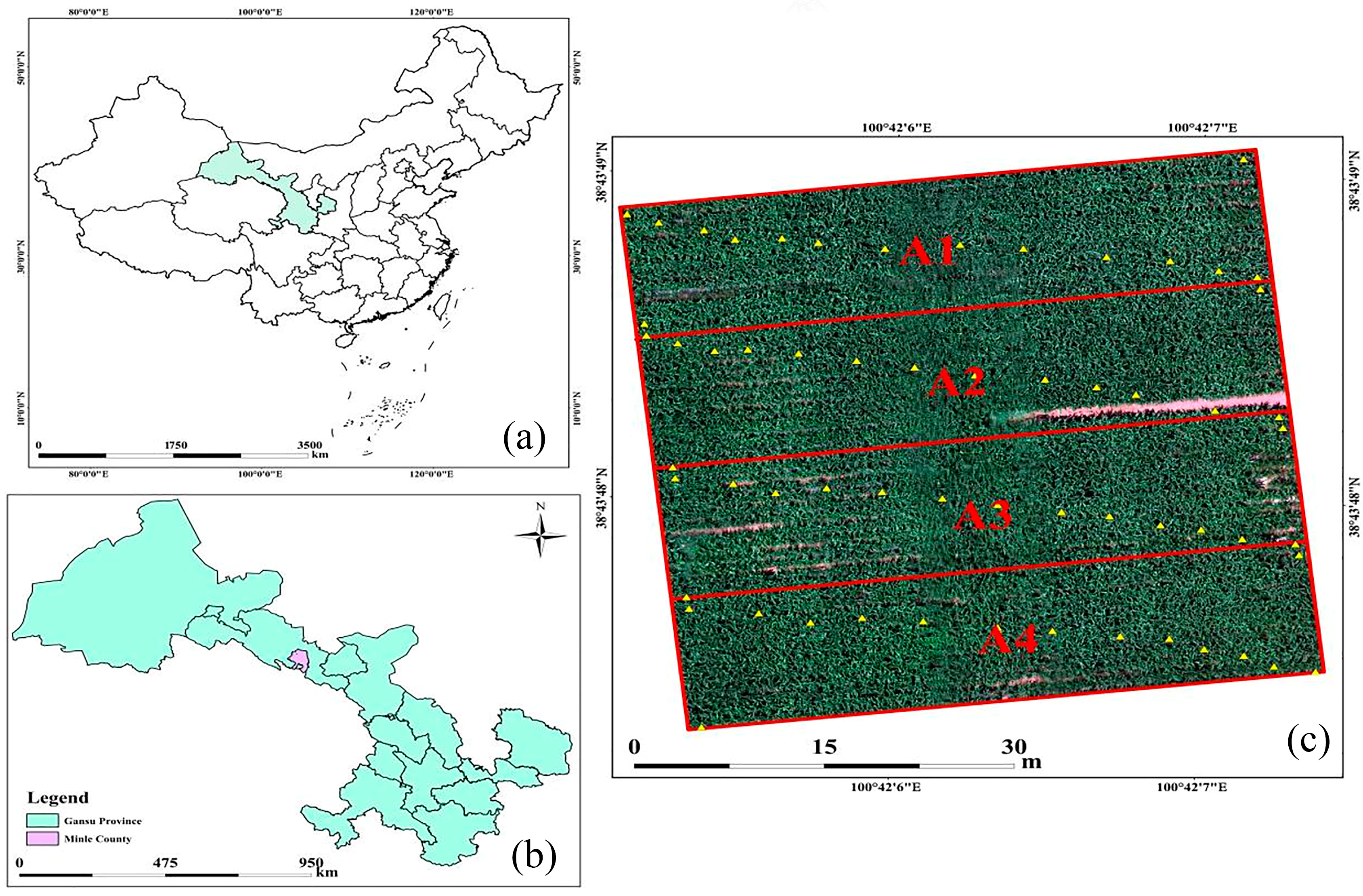
2.1. Overview of the Study Area

This study was conducted at the Huari Farm experimental station in Gansu Province from April to October 2022. The study area is located in Zhangye City, which has a cultivated land area of 355,660 ha, making it a typical oasis irrigation agricultural region and one of the key areas for silage corn cultivation in Gansu. Figure 1 illustrates the geographical location and extent of the study area, as well as the distribution of experimental plots and sampling points. The region lies within the Heihe River Basin and is classified under the temperate continental desert steppe climate zone. The average elevation is 1629 m, with a frost-free period of 140 days. The region receives an average annual solar radiation of 2794 h, and the light and heat resources are relatively abundant. The average annual precipitation is 290 mm, and the mean annual temperature ranges from 3.4 to 5.6 °C. The soil in the area is predominantly foreign soil, with sandy soil as the main type. The organic carbon content in the plow layer is 5.96 g·kg−1, the total nitrogen content is 0.70 g·kg−1, the total phosphorus content is 0.65 g·kg−1, the available potassium content is 6.89 g·kg−1, and the bulk density is 1.18 g·cm−3.

2.2. Experimental Design

The silage corn was sown on 27 April 2022, with emergence occurring around 10 May. The harvest date was scheduled for 26 September, resulting in a total growing period of 144 days. During the planting process, a mulch sowing technique was employed, with a sowing depth of approximately 5 cm. The plant spacing was maintained at 25 cm, and the row spacing was set at 50 cm, with the rows oriented from east to west to optimize light utilization. A randomized block design was used for the experiment, with four nitrogen fertilizer treatments (urea), namely N1 (311 kg/hm2), N2 (280 kg/hm2), N3 (249 kg/hm2), and N4 (218 kg/hm2), applied in five split doses. The experimental plots utilized a full-film double-ridge furrow sowing technique with a planting density of 113,100 plants/hm2. Irrigation was carried out using drip irrigation under the film, with an internal-banded, patch-type drip tape with a diameter of 16 mm, a wall thickness of 0.2 mm, an emitter spacing of 300 mm, and an emitter flow rate of 2.2 L/h. The drip tape was laid parallel to the planting direction of the silage corn, with a spacing of 60 cm. Irrigation started in early May and ended in early September, with other management practices following conventional field methods. To prevent interference between plots, a 1 m-wide isolation belt was established around each plot. Fertilization was mainly carried out before sowing, with 4500 kg/hm2 of cow manure applied as the base fertilizer. Fertilizer was applied using a hydraulic pump device and was incorporated during irrigation. Urea (46% N content) was used for nitrogen fertilization. Additionally, during different growth stages, phosphorus (P2O5 content 44.06%) and potassium (K2O content 57%) fertilizers were applied according to the traditional schedule. The total amounts of phosphorus and potassium fertilizers applied were 146 kg/hm2 and 107 kg/hm2, respectively. Fertilization occurred before the jointing stage (2 weeks before jointing) (5.9%), at the jointing stage (64.7%), and at the tasseling stage (29.4%), as detailed in Table 1. Other management practices were consistent with those used in conventional fields.

2.3. Data Collection and Processing for the Experiment

2.3.1. UAV Multispectral Remote Sensing Imagery Acquisition and Processing

The experiment utilized a DJI M300 UAV, which has a maximum payload capacity of 2.7 kg, a maximum flight time of 55 min, a maximum flight speed of 23 m/s, and a maximum operating altitude of 7000 m. The UAV is capable of withstanding winds up to 15 m/s and operates within a temperature range of −20 °C to 50 °C. It supports dual-frequency communication at 2.4/5.8 GHz and features the OcuSync Industry Edition transmission system, offering a control range of up to 15 km. The six bands used were 450 nm, 555 nm, 660 nm, 720 nm, 750 nm, and 840 nm. Data collection was carried out under clear skies with no wind, with the UAV flying at a height of 30 m. The flight period was from 12:00 to 15:00 local time. The multispectral camera was oriented directly downward, with forward and sideward overlaps set to 80% and 75%, respectively. All images were captured along a fixed flight path. The reflectance values of the diffuse reflectance board at central wavelengths are shown in Table 2, and Figure 2 illustrates the data collection and processing workflow.
In this study, data collection was conducted on 18 May (seedling stage), 1 July (jointing stage), 4 August (tasseling stage), and 7 September (maturity stage). The collected data were processed using Pix4D Mapper software (v4.5.6) to stitch the multispectral images into a complete image of the experimental area. Then, the reflectance images were radiometrically corrected using a diffuse reflectance panel, generating accurate crop reflectance information. To ensure that the geographic coordinates in the image aligned with the true geographic coordinates, the stitched images were geometrically corrected by manually registering the vector files of four ground control points and four geometric control panels. Radiometric and geometric corrections were successfully completed. The RMSE for radiometric correction was 0.03, and the coordinate deviation for geometric correction was 1.2 m, indicating that the correction process achieved high precision. The quality of the corrected images significantly improved, providing a reliable data foundation for subsequent inversion analysis. Finally, the five single-band reflectance images were merged into a six-band reflectance image using the layer-stacking function in ENVI software (ENVI 5.3), facilitating subsequent image processing and the extraction of reflectance data from various sample areas.

2.3.2. Soil Sampling and Total Nitrogen Determination

After the UAV image collection, 12 sampling points were selected along the diagonals of each experimental plot. Soil samples were collected from the rhizosphere of silage corn at different growth stages using a soil auger, with samples taken from the 0–30 cm soil layer. The samples were air-dried in a clean and well-ventilated environment, avoiding direct sunlight. During the drying process, the samples were regularly turned to ensure even drying. Once fully air-dried, the samples were sieved through a 0.25 mm mesh to prepare for total nitrogen (TN) determination. Another portion of the samples was stored at low temperature for future use. The total nitrogen content (TN) was measured using a rapid determination method for soil available nutrients, with 48 samples collected at each growth stage: seedling, jointing, tasseling, and maturity. The TN measurement was carried out using the TY-type soil nutrient quick tester, following the comparative study of various rapid determination methods for soil available nutrients by Wang Hui [22].

2.4. Construction and Selection of Vegetation Indices

Vegetation indices are mathematical expressions used in remote sensing to describe and quantify characteristics such as vegetation growth status and coverage [23]. These indices utilize the spectral reflection properties of vegetation in visible light, near-infrared, and other wavelengths. Through specific computational methods, dimensionless values are derived to reflect the growth state and coverage of the vegetation. Vegetation indices are mathematical expressions used in remote sensing to describe and quantify vegetation growth status and canopy characteristics [24]. In the inversion of soil total nitrogen content, vegetation indices indirectly reflect soil nitrogen status by quantifying the spectral characteristics of vegetation, especially when soil reflectance is obscured by the vegetation canopy. Under such conditions, vegetation indices become essential tools for soil nitrogen inversion. For instance, the Normalized Difference Vegetation Index (NDVI) and the Enhanced Vegetation Index (EVI), based on spectral reflectance in the red and near-infrared bands, are sensitive to chlorophyll content and biomass, thereby indirectly reflecting soil nitrogen conditions. In this study, we selected GOSAVI, GNDVI, GDVI, DVI, CVI, CIRE, GSAVI, MNDI, MTCI, NDRE, NDVI, NNI, NRI, OSAVI, RENDVI, SAVI, GRVI, NREI, red, rededge1, rededge2, nir, green, and blue as the core vegetation indices due to their high applicability under vegetation-covered conditions and their ability to enhance the accuracy and robustness of soil nitrogen inversion models. By integrating multispectral data with machine learning algorithms, this study further optimized the application of vegetation indices in soil nitrogen inversion, providing a solid theoretical foundation and methodological guidance for future research. These indices, which are quantitative indicators derived from mathematical combinations of different spectral bands from multispectral imagery, effectively capture vegetation physiological status and canopy coverage. The calculation formulas are presented in Table 3.

2.5. Model Construction and Analysis

Three machine learning algorithms, including backpropagation neural network (BPNN), random forest regression (RF), and partial least squares regression (PLSR), were employed to construct soil total nitrogen inversion models. BPNN is a multilayer feedforward neural network that optimizes network parameters using the error backpropagation algorithm [25,26]. This network typically consists of an input layer, one or more hidden layers, and an output layer, with each layer containing a specific number of neurons. The advantage of BPNN lies in its ability to automatically adjust the connection weights between neurons during the training process, enabling the approximation and generalization of complex nonlinear functions. RF is an ensemble learning method that builds multiple decision trees and combines their predictions to achieve high accuracy in continuous value forecasting. It enhances the model’s robustness by utilizing the randomness of the data and features, while also evaluating feature importance, making it an effective tool for complex regression tasks [27]. PLSR is a multivariate analysis technique, particularly suitable for spectral data analysis. It identifies latent variables in spectral data that are most strongly correlated with soil total nitrogen content and can handle multicollinearity issues within the data [28].

2.6. Model Accuracy Evaluation

Seventy percent of the soil samples from the maize root zone (i.e., 32 samples) were used as the training set, while the remaining samples served as the validation set. The model’s accuracy was evaluated by assessing the coefficient of determination (R2) and root mean square error (RMSE) for both the training and the validation sets. The coefficient of determination (R2), a quantitative measure of how well the model fits the ideal line y = x, ranges between 0 and 1. A higher R2 indicates better prediction accuracy and stability, with greater agreement between the observed and predicted values. The RMSE directly reflects the level of error in the model’s predictions. A smaller RMSE value suggests stronger model performance and higher predictive accuracy [29]. Together, these metrics provide a comprehensive evaluation of the model’s performance, offering strong guidance for model optimization and selection.

3. Results and Analysis

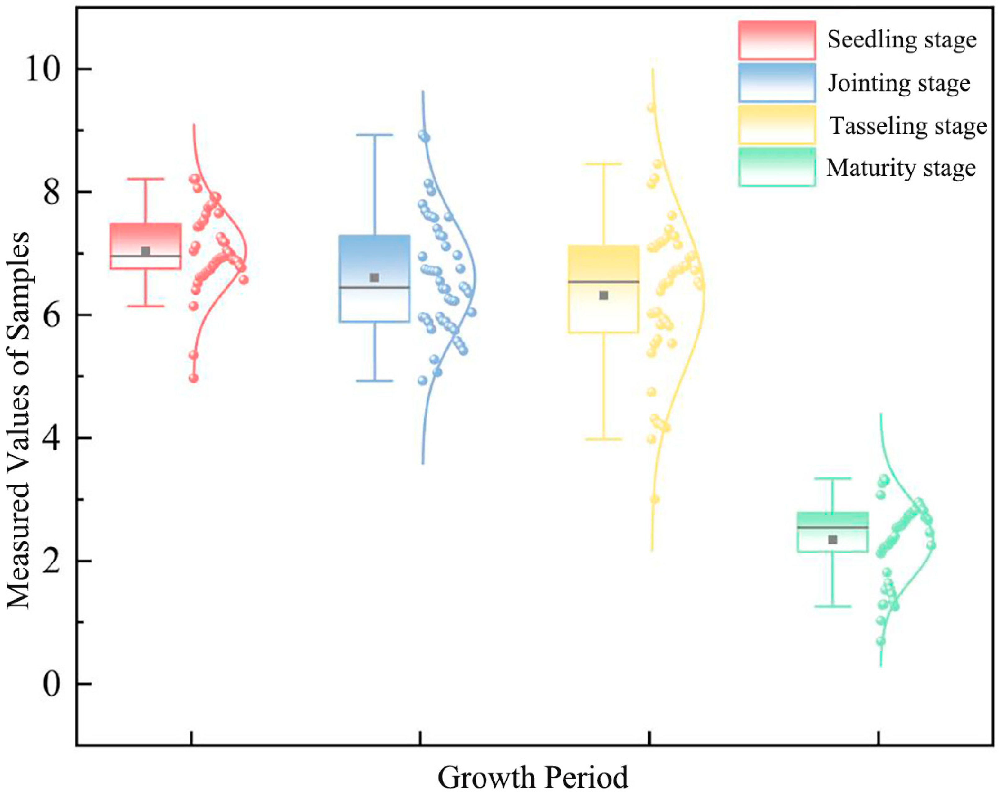
3.1. Statistical Analysis of Soil Total Nitrogen Content

A total of 48 soil samples from the rhizosphere of silage maize at the 0–30 cm depth were collected at four growth stages. These samples were subjected to detailed analysis of their total nitrogen content. The nitrogen content in the rhizosphere soil of silage maize showed a gradual decrease throughout the growing stages. As shown in Table 4, the descriptive analysis of soil total nitrogen content is presented. As shown in Table 4, the coefficient of variation for the total nitrogen content of the rhizosphere soil samples remained below 0.4 in all four growth stages, indicating low variability. Figure 3 is the statistical result of soil total nitrogen. Although the maximum and minimum values of total nitrogen (TN) content for most samples fell within the expected reasonable range, a few outliers were observed in the box plot. These outliers, confirmed through Grubbs’ test, may be attributed to sampling errors or localized uneven fertilization. To ensure data reliability, the outliers were not excluded from subsequent analyses; however, their impact on the model results was thoroughly evaluated and is discussed in the discussion section. All samples were representative and provided a comprehensive and accurate reflection of soil characteristics, making them suitable for inclusion in the complete model dataset for further analysis.

3.2. Selection of Sensitive Variables

To enhance the accuracy of UAV-based multispectral remote sensing models for soil total nitrogen (TN) inversion under vegetation-covered conditions, this study focused on maize-covered fields as the research object. Multispectral images of the study area were acquired using a UAV, and surface soil samples were collected simultaneously for laboratory determination of soil TN content. Subsequently, three methods—grey relational analysis (GRA), variable importance in projection (VIP), and support vector machine recursive feature elimination (SVM-RFE)—were employed to select sensitive variables from spectral reflectance and spectral indices. The selected sensitive variables were then used as modeling factors to develop soil TN inversion models using partial least squares regression (PLSR), backpropagation neural networks (BPNNs), and random forest (RF), respectively. By comparing and analyzing the accuracy of different inversion models, the optimal model for soil TN inversion was evaluated and selected.

3.2.1. Comparative Analysis and Optimization Based on Multiple Spectral Index Selection Methods

In this study, the SVM-RFE algorithm was used to select 24 spectral indices, including vegetation indices and spectral bands (implemented based on MATLAB R2018a). By sequentially increasing the number of selected features, it was found that the best model accuracy was achieved when 18 features were retained. To minimize the impact of the number of selected features on model accuracy, 18 spectral indices were chosen as input features for the model in each growth stage. SVM-RFE ranks features based on the accuracy of the SVM machine learning model and removes the least important features. The remaining features are used to retrain the model for the next iteration, continuing until no features remain. The top-ranked feature alone is not necessarily the optimal subset; rather, it is the combination of feature variables that enables the model to achieve optimal performance. Through iterative process, the number of retained features is gradually reduced, resulting in an importance ranking, as shown in Table 5. Table 5 shows the ranking of the importance of the spectral index filtered by the SVM-RFE.
Using MATLAB R2019a software, a variable importance in projection (VIP) analysis was conducted to evaluate the relationship between 24 variables and soil total nitrogen (TN) content, generating the VIP scores for each variable, as shown in Table 6. Variables with VIP scores greater than 1 were selected as independent variables for the inversion models at different growth stages. The selected variables wee as follows: for the seedling stage, GOSAVI, GNDVI, GDVI, CIRE, GSAVI, MNDI, MTCI, NDRE, NDVI, OSAVI, SAVI, NREI, rededge1, rededge2, and nir; for the jointing stage, GOSAVI, GNDVI, GDVI, GSAVI, MTCI, NDRE, NDVI, OSAVI, SAVI, NREI, rededge1, and nir; for the tasseling stage, GOSAVI, GNDVI, CIRE, GSAVI, NDRE, NDVI, OSAVI, SAVI, NREI, rededge1, rededge2, nir, and green; and for the maturity stage, GOSAVI, GNDVI, GDVI, GSAVI, MTCI, SAVI, NDRE, NDVI, rededge1, and nir. Table 6 presents the VIP scores of the variables for each growth stage.
In MATLAB R2019a software, grey relational degree (GCD) analysis was performed between 24 spectral variables and soil total nitrogen (TN) content. The results of the grey relational degree analysis are shown in Table 7. To achieve variable selection, the GCD threshold for sensitive variables was set at 0.8. The final selected variables for use as independent variables in the inversion models for different growth stages were as follows: for the seedling stage, GNDVI, GDVI, NDRE, NDVI, rededge1, rededge2, and nir; for the jointing stage, GNDVI, GDVI, CIRE, NDRE, NDVI, OSAVI, rededge1, rededge2, and nir; for the tasseling stage, GNDVI, GDVI, CIRE, NDRE, NDVI, OSAVI, rededge1, rededge2, nir, and green; and for the maturity stage, GOSAVI, GNDVI, GSAVI, NDRE, NDVI, OSAVI, rededge1, and nir. Table 7 presents the grey relational degree (GCD) scores of the variables for each growth stage based on MATLAB.

3.2.2. Correlation Analysis of Spectral Indices

Pearson correlation analysis is a statistical tool used to quantify the strength and direction of the linear relationship between two continuous variables [30,31]. In this study, this method was applied to assess the linear correlation between the selected spectral indices and the soil nitrogen content data. Specifically, we calculated the correlation coefficient between the spectral index values and the measured nitrogen content in the soil samples to reveal the degree of their linear dependence. As shown in Figure 4, throughout the four growth stages, the spectral indices consistently passed the significance test, with some indices showing a very high level of significance (p < 0.001) in their correlation with the corresponding attributes. This indicates that the spectral indices selected by the SVM-RFE method are suitable for developing predictive models or conducting further research.

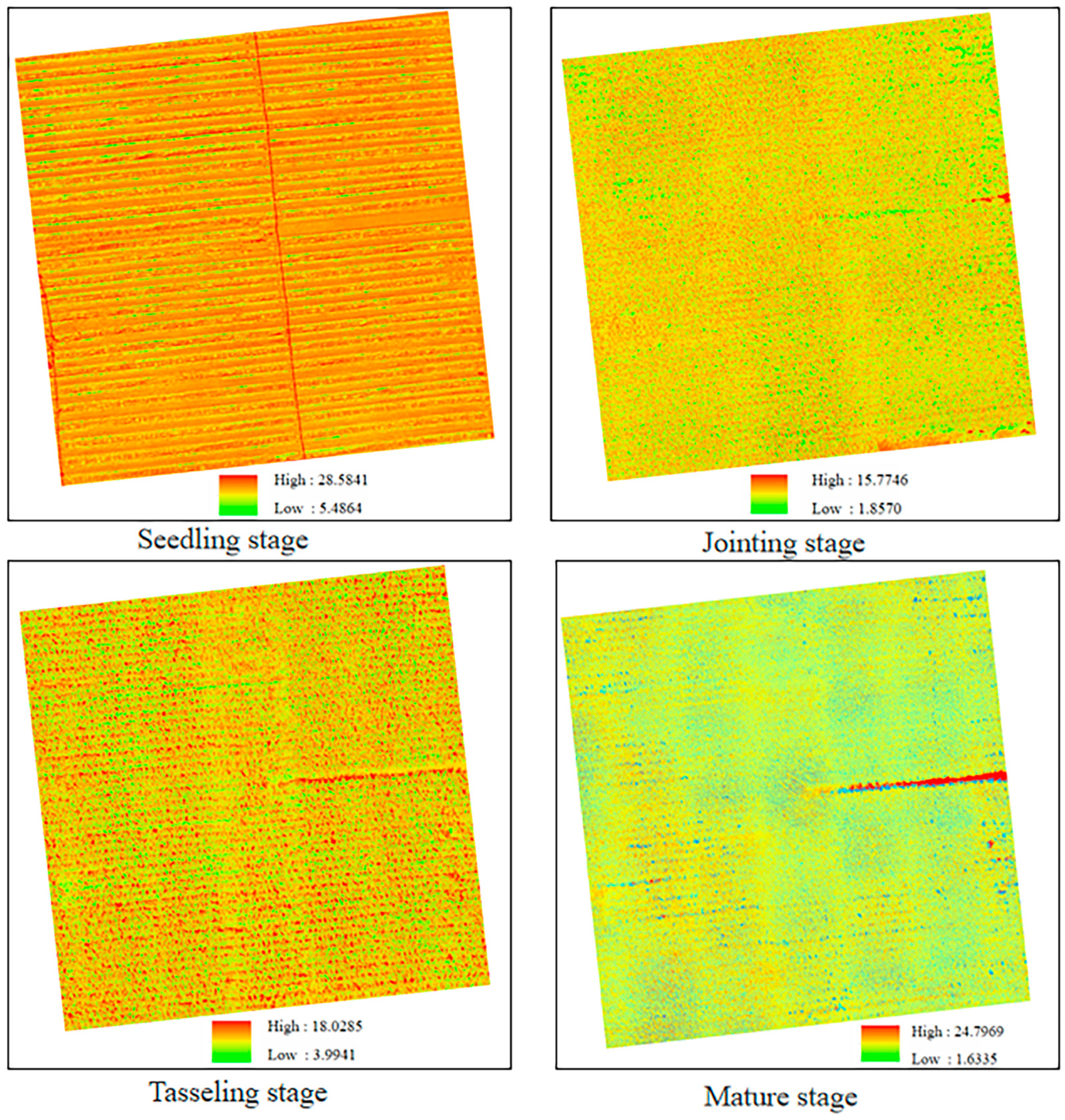
3.2.3. Post-Selection Model Inversion Analysis

The model was constructed using 18 spectral indices selected based on the SVM-RFE algorithm. Table 8 integrates the results of soil total N inversion in different periods before and after screening based on the SVM-RFE algorithm. As shown in Table 8, the model accuracy achieved with the selected indices outperformed that of the model built using unselected spectral indices. From both Table 8 and Figure 5, it can be seen that the R2 values for the model inversion of silage corn rhizosphere soil before the index selection ranged from 0.362 to 0.500, from 0.372 to 0.416, from 0.417 to 0.581, and from 0.439 to 0.608, while the RMSE values ranged from 0.967 to 1.280, from 0.474 to 0.617, from 0.420 to 0.522, and from 0.379 to 0.529, respectively. After the selection, the R2 values ranged from 0.465 to 0.552, from 0.394 to 0.458, from 0.465 to 0.630, and from 0.480 to 0.663, while the RMSE values ranged from 0.952 to 1.231, from 0.452 to 0.681, from 0.349 to 0.552, and from 0.281 to 0.494, respectively. These results indicate that, from a modeling perspective, PLSR provides the best inversion performance, with an R2 of 0.663 and RMSE of 0.281, followed by RF. From the perspective of the inversion period, the optimal time for inversion of silage corn rhizosphere soil nitrogen content is at the maturity stage, followed by the tasseling stage, with the worst performance observed at the seedling stage. Figure 6 presents the Comparison between the measured values and the predicted values of total soil nitrogen content.
This study produced soil total nitrogen (TN) distribution maps for different growth stages in the study area, as shown in Figure 7. From Figure 7, it can be observed that the total nitrogen content decreased in the following order: seedling stage > tasseling stage > jointing stage > maturity stage. This result aligns with the laboratory measured values. During the seedling stage, plant nitrogen absorption was limited, and the rhizosphere soil nitrogen content was relatively high. In the tasseling stage, although the plants had a higher nitrogen demand, there was still a certain amount of nitrogen available in the soil, and the duration of this stage was relatively short, so nitrogen consumption was not as rapid as in the jointing stage, resulting in intermediate nitrogen content. During the jointing stage, maize growth accelerated, and the nitrogen demand increased sharply. The plants absorbed large amounts of nitrogen from the rhizosphere soil, leading to a significant decrease in soil nitrogen content. By the maturity stage, plant growth had slowed down, a large amount of nitrogen had already been consumed, and some nitrogen had been transferred to the grains, resulting in the lowest rhizosphere soil nitrogen content among all growth stages.

4. Discussion

The model in this study performed well on data from the Huari Farm in Minle County, Gansu Province, in 2022. However, since the data were only from a single location and a single year, the model’s generalizability may be limited. For example, variations in climate conditions, soil types, or years may affect model accuracy. To further validate the model’s generalizability, data from 2023 and 2024 were obtained for cross-year validation. The results show that the model maintained high accuracy for the 2023 and 2024 data. In 2023, soil total nitrogen inversion models were constructed using three methods: BP neural network (BPNN), partial least squares regression (PLSR), and random forest (RF). The results show that the coefficient of determination (R2) for the modeling and validation sets reached 0.485, 0.452, and 0.550, and 0.479, 0.458, and 0.543, respectively. In 2024, models were again constructed using BPNN, PLSR, and RF, with the R2 for the modeling and validation sets reaching 0.501, 0.475, and 0.600, and 0.433, 0.412, and 0.499, respectively. These results indicate that the models had high reliability and stability, demonstrating good applicability across different years. However, we also observed a slight decrease in model accuracy under extreme climate conditions, which may be related to the impact of climate variability on soil nitrogen dynamics. Future research should expand to more regions and years to further validate the robustness of the model and explore methods to enhance its generalizability through multi-source data or advanced algorithms.
Crop canopy spectral reflectance is highly sensitive to soil total nitrogen content. By utilizing vegetation indices, a relationship can be established between the indices and the measured soil nitrogen levels, thus enabling the inversion of soil nitrogen content. This study focuses on the rhizosphere soil of silage maize and investigates the inversion of soil total nitrogen content in the 0–30 cm soil layer across different growth stages of maize. Using a drone-mounted multispectral camera, we developed inversion models for soil nitrogen content across multiple periods and models. By performing inversion in small experimental areas, we were able to quickly obtain soil total nitrogen content across the entire agricultural region at various stages of the growing season. In this study, although the boxplot displayed a small number of outliers, we confirmed through the Grubbs test that these outliers did not significantly deviate from the overall distribution. To assess the impact of outliers on the model results, we conducted a sensitivity analysis. After removing the outliers, the model’s RMSE changed from 0.28 to 0.27, a change of less than 4%, indicating that the impact of outliers on the results was negligible. Therefore, we chose to retain these outliers to maintain the integrity of the data.
The SVM-RFE variable selection method enables the identification of vegetation indices with high correlation. Most of the selected spectral indices are vegetation indices, primarily because the spectral characteristics of crops differ significantly due to variations in crop types and vegetation cover [32,33]. As a result, the spectral indices derived from different spectral bands exhibited considerable differences. This study also found that the R2 values of the models based on SVM-RFE-selected indices were higher than those before selection, indicating more accurate inversion results. A similar conclusion was proposed by Zhao Wenju in his study of soil salinity inversion models for different soil depths under various crop covers using UAV-based multispectral images [34]. It is evident that inversion models based on SVM-RFE-selected indices perform better than those based on unselected indices. This improvement is primarily due to the SVM-RFE algorithm, which iteratively trains the SVM while removing insignificant features, effectively selecting key predictive features and eliminating redundancy and noise, thereby significantly enhancing the model’s generalization ability.
Numerous experts and scholars have utilized partial least squares regression (PLSR) and random forest regression (RF) models to invert crop characteristics. By comparing the performance of different models, the optimal model can be selected to enhance the accuracy of the inversion results. For instance, Guo et al. applied PLSR to predict the winter wheat yield, achieving a root mean square error (RMSE) of 0.903 g/m2 [35]. Similarly, Li used the PLSR model to predict nitrogen content in apple leaves, with a root mean square error of prediction (RMSEP) of 0.031 mg/g [36]. Wang Qianlong and colleagues found that combining fuzzy k-means clustering with PLSR yielded better results for soil [37]. Therefore, it is feasible to use PLSR to invert the total nitrogen content in the soil surface layer. In addition, Yang Fuqin et al. [38] selected image indices with a high correlation to the nitrogen nutrition index of winter wheat based on multicollinearity, and then constructed an inversion model using partial least squares regression (PLSR). The root mean square error (RMSE) for the training set reached 0.0858, while the RMSE for the validation set was 0.1871, indicating high prediction accuracy. LAURIN et al. [39] applied PLSR and used hyperspectral data combined with vegetation indices to model biomass in the African tropical rainforest. They found that the improved model (R2 = 0.70) outperformed the regression model, which did not account for multicollinearity (R2 = 0.64). Furthermore, Liu et al. [40] found that the BP neural network model performed excellently when using UAV hyperspectral data to quantitatively model nitrogen content in winter wheat leaves. Our study, however, found that the PLSR model performed best when constructing a model for total nitrogen content in the rhizosphere soil of silage maize, compared to the RF and BPNN regression models. Thus, models based on the PLSR algorithm exhibit high inversion accuracy, good stability, and strong resistance to overfitting. However, when inverting nitrogen content in different soils and crops, it is essential to select various models based on different climatic characteristics and environmental factors.
Furthermore, this study compared different models across four growth stages and found that the R2 values of all models progressively increased from the seedling stage to the maturity stage. This not only indicates that the inversion accuracy of the selected models improved significantly as the maize growth period advanced, but also reveals the changes in the physiological and spectral characteristics of maize throughout its growth. Notably, the R2 value at maturity reached a maximum of 0.663. This result not only validates the effectiveness of the selected models in the later stages of maize growth, but also provides strong support for future optimization of inversion algorithms and enhancement of model accuracy.
This study focuses on the inversion model of surface total nitrogen content in the rhizosphere soil of silage maize at different growth stages based on UAV multispectral imagery. Although satisfactory inversion results were obtained, certain limitations remain. The influence of multi-source remote sensing and environmental factors, such as the effect of meteorological conditions on nitrogen content, was not considered and requires further investigation. Additionally, the model is based solely on one year of data. In the future, combining satellite remote sensing, incorporating more parameters, and integrating multi-source remote sensing data with physiological and biochemical parameters may enhance both the accuracy and the applicability of the model, providing support for agricultural monitoring in the arid Hexi region. In addition, due to experimental constraints, no physical isolation strips were set up. To reduce interference between treatment plots, we left sufficient space between plots (e.g., more than 1 m apart). Potential cross-interference was considered in the data analysis, and statistical methods were used to evaluate the significance of differences between treatments. Nonetheless, we acknowledge that the lack of isolation strips may have led to the movement of water and nutrients between plots, which could have affected the distinction between different nitrogen fertilizer treatment levels. Future studies are recommended to establish isolation strips or adopt other effective measures to reduce interference and improve the accuracy and reliability of experimental results.

5. Conclusions

This study collected total nitrogen content in the rhizosphere soil of silage maize at different growth stages. The SVM-RFE algorithm was used to select spectral indices, which were then combined with three machine learning algorithms: BPNN, RF, and PLSR, to perform soil total nitrogen inversion under silage maize coverage. The following conclusions were drawn from the study:
(1) The SVM-RFE (support vector machine–recursive feature elimination) variable selection method was used for the effective screening of spectral variables. The results show that the inversion model constructed using the selected variables significantly outperformed the model that did not undergo variable selection. This validates the effectiveness of the SVM-RFE method in feature dimensionality reduction and demonstrates its suitability for high-precision inversion of soil total nitrogen content.
(2) For the inversion of soil total nitrogen content within the same growth stage, the performance of three model algorithms, namely BPNN, RF, and PLSR, was compared. The results indicate that all models exhibited good robustness, but the PLSR model had a significantly higher coefficient of determination (R2) than the other two models. Additionally, its accuracy evaluation metrics, such as root mean square error (RMSE), were generally superior to those of the other models. Therefore, considering all performance indicators, the PLSR model was confirmed as the optimal choice for inverting total nitrogen content in the rhizosphere soil of silage maize.
(3) The PLSR models established at specific soil depths for different growth stages were compared in terms of their accuracy in inverting total nitrogen content in the rhizosphere soil of silage maize. The model for the maturity stage performed the best, significantly outperforming those for the tasseling and jointing stages, while the model for the seedling stage had the poorest inversion performance. This suggests that the maturity stage is the optimal period for inverting total nitrogen content in the rhizosphere soil of silage maize in the study area.

Author Contributions

Writing—original draft preparation, H.Y.; project administration, J.Y. and G.L.; writing—review and editing, H.Y. and X.Y.; data curation, J.L.; supervision, W.M.; software, H.Y., Q.D., X.L. and K.C. All authors have read and agreed to the published version of the manuscript.

Funding

This work was supported by the Gansu Provincial Science and Technology Major Special Project (24ZD13NA019); Central guide local science and technology development special funds (24ZYQA023); National Natural Science Foundation of China (42461060; 42307564); Gansu Provincial Key Research and Development Project for Ecological Civilization Construction (24YFFA059; 24YFFA056); Gansu Provincial Department of Education Industry Support Plan Project (2025CYZC-042; 2022CYZC-41).

Data Availability Statement

The data presented in this study are available on request from the corresponding author due to the datasets generated and analyzed during the current study not being publicly available due to the limited availability of some data.

Acknowledgments

We sincerely thank the editor and reviewers for their time and effort in reviewing our work.

Conflicts of Interest

The authors declare that they have no known competing financial interests or personal relationships that could have appeared to influence the work reported in this paper.

References

  1. Zhang, X.; Davidson, E.A.; Mauzerall, D.L.; Searchinger, T.D.; Dumas, P.; Shen, Y. Managing nitrogen for sustainable development. Nature 2015, 528, 51. [Google Scholar]
  2. Spiertz, J.H.J. Nitrogen, sustainable agriculture and food security: A review. Agron. Sustain. Dev. 2010, 30, 43–55. [Google Scholar] [CrossRef]
  3. Rütting, T.; Aronsson, H.; Delin, S. Efficient use of nitrogen in agriculture. Nutr. Cycl. Agroecosystems 2018, 110, 1–5. [Google Scholar] [CrossRef]
  4. Pearcy, R.W.; Ehleringer, J.R.; Mooney, H.A.; Rundel, P.W.; Binkley, D.; Vitousek, P. Soil Nutrient Availability. Plant Physiol. Ecol. 1989. [Google Scholar] [CrossRef]
  5. Assefa, S.; Tadesse, S. The principal role of organic fertilizer on soil properties and agricultural productivity-a review. Agric. Res. Technol. Open Access J. 2019, 22, 1–5. [Google Scholar]
  6. Savci, S. Investigation of effect of chemical fertilizers on environment. Apcbee Procedia 2012, 1, 287–292. [Google Scholar]
  7. Liu, J.S.; Dai, J.; Liu, Y.; Guo, X.; Wang, Z.H. Effects of excessive nitrogen fertilization on soil organic carbon and nitrogen and nitrogen supply capacity in dryland. J. Plant Nutr. Fertil. 2015, 21, 112–120. [Google Scholar]
  8. Chen, G.; Yang, K.; Meng, Y.; Liu, D.; Jiang, Y.; Li, X. Screening and genetic characteristics of breeding materials of silage corn. Anim. Feed. Sci. Engl. Ed. 2011, 3, 4. [Google Scholar]
  9. Stone, M.L.; Solie, J.B.; Raun, W.R.; Whitney, R.W.; Taylor, S.L.; Ringer, J.D. Use of spectral radiance for correcting in-season fertilizer nitrogen deficiencies in winter wheat. Trans. ASAE 1996, 39, 1623–1631. [Google Scholar] [CrossRef]
  10. Peng, Y.; Wang, L.; Zhao, L.; Liu, Z.; Lin, C.; Hu, Y.; Liu, L. Estimation of soil nutrient content using hyperspectral data. Agriculture 2021, 11, 1129. [Google Scholar] [CrossRef]
  11. Miao, Y.; Mulla, D.J.; Hernandez, J.A.; Wiebers, M.; Robert, P.C. Potential impact of precision nitrogen management on corn yield, protein content, and test weight. Soil Sci. Soc. Am. J. 2007, 71, 1490–1499. [Google Scholar]
  12. Cassman, K.G.; Dobermann, A.; Walters, D.T. Agroecosystems, nitrogen-use efficiency, and nitrogen management. AMBIO J. Hum. Environ. 2002, 31, 132–140. [Google Scholar] [CrossRef] [PubMed]
  13. Ma, B.L.; Biswas, D.K. Precision nitrogen management for sustainable corn production. Sustain. Agric. Rev. Cereals 2015, 33–62. [Google Scholar]
  14. Mu, H.B. Research on the Application of Near-Infrared Spectroscopy in the Evaluation of Nutritional Quality of Corn and Silage Quality. Doctoral Dissertation, Inner Mongolia Agricultural University, Hohhot, China, 2008. [Google Scholar]
  15. Li, Y.Q.; Yang, D.H.; Dao, J.; Wang, J.X. Inversion of main nutrient contents in red soil of mountain plain based on UAV multispectral remote sensing. J. Jiangxi Agric. Sci. 2021, 33, 63–67. [Google Scholar]
  16. Tao, P.F.; Wang, J.H.; Li, Z.Z.; Zhou, P.; Yang, J.J.; Gao, F.Q. Research on Inversion Models of Soil Nutrient Content Based on Hyperspectral Imaging. Geol. Resour. 2020, 29, 68–75+84. [Google Scholar]
  17. Thompson, L.J.; Puntel, L.A. Transforming unmanned aerial vehicle (UAV) and multispectral sensor into a practical decision support system for precision nitrogen management in corn. Remote Sens. 2020, 12, 1597. [Google Scholar] [CrossRef]
  18. Sáez-Plaza, P.; Michałowski, T.; Navas, M.J.; Asuero, A.G.; Wybraniec, S. An overview of the Kjeldahl method of nitrogen determination. Part I. Early history, chemistry of the procedure, and titrimetric finish. Crit. Rev. Anal. Chem. 2013, 43, 178–223. [Google Scholar]
  19. Maes, W.H.; Steppe, K. Perspectives for remote sensing with unmanned aerial vehicles in precision agriculture. Trends Plant Sci. 2019, 24, 152–164. [Google Scholar] [CrossRef]
  20. Jiachen, H.; Jing, H.; Gang, L.; Weile, L.; Zhe, L.; Zhi, L. Inversion analysis of soil nitrogen content using hyperspectral images with different preprocessing methods. Ecol. Inform. 2023, 78, 102381. [Google Scholar]
  21. Liakos, K.G.; Busato, P.; Moshou, D.; Pearson, S.; Bochtis, D. Machine learning in agriculture: A review. Sensors 2018, 18, 2674. [Google Scholar] [CrossRef]
  22. Brereton, R.G.; Lloyd, G.R. Support vector machines for classification and regression. Analyst 2010, 135, 230–267. [Google Scholar]
  23. Guo, J.; Wang, K.; Jin, S. Mapping of soil pH based on SVM-RFE feature selection algorithm. Agronomy 2022, 12, 2742. [Google Scholar] [CrossRef]
  24. Lyon, J.G.; Yuan, D.; Lunetta, R.S.; Elvidge, C.D. A change detection experiment using vegetation indices. Photogramm. Eng. Remote Sens. 1998, 64, 143–150. [Google Scholar]
  25. Dimkpa, C.; Bindraban, P.; McLean, J.E.; Gatere, L.; Singh, U.; Hellums, D. Methods for rapid testing of plant and soil nutrients. Sustain. Agric. Rev. 2017, 1–43. [Google Scholar]
  26. Gao, L.; Wang, X.; Johnson, B.A.; Tian, Q.; Wang, Y.; Verrelst, J.; Mu, X.; Gu, X. Remote sensing algorithms for estimation of fractional vegetation cover using pure vegetation index values: A review. ISPRS J. Photogramm. Remote Sens. 2020, 159, 364–377. [Google Scholar] [PubMed]
  27. Wang, F.M.; Huang, J.F.; Tang, Y.L.; Wang, X.Z. New vegetation index and its application in estimating leaf area index of rice. Rice Sci. 2007, 14, 195. [Google Scholar]
  28. Zhao, W.; Ma, H.; Zhou, C.; Zhou, C.; Li, Z. Soil salinity inversion model based on BPNN optimization algorithm for UAV multispectral remote sensing. IEEE J. Sel. Top. Appl. Earth Obs. Remote Sens. 2023, 16, 6038–6047. [Google Scholar]
  29. Ju, C.; Chen, C.; Li, R.; Zhao, Y.; Zhong, X.; Sun, R.; Liu, T.; Sun, C. Remote sensing monitoring of wheat leaf rust based on UAV multispectral imagery and the BPNN method. Food Energy Secur. 2023, 12, e477. [Google Scholar]
  30. Manafifard, M. A new hyperparameter to random forest: Application of remote sensing in yield prediction. Earth Sci. Inform. 2024, 17, 63–73. [Google Scholar]
  31. Zhang, Z.; Liu, Z.; Guo, Y.; Han, J.; Li, Y. The application of partial least squares to Tibet's grassland biomass monitoring by remote sensing. Acta Agrestia Sin. 2009, 17, 735–739. [Google Scholar]
  32. Chen, L.; Huang, J.F.; Wang, F.M.; Tang, Y.L. Comparison between back propagation neural network and regression models for the estimation of pigment content in rice leaves and panicles using hyperspectral data. Int. J. Remote Sens. 2007, 28, 3457–3478. [Google Scholar]
  33. Wang, J.; Zhang, F.; Wang, Y.; Fu, Y.; Liang, Y. Identification of Salt Tolerance Genes in Rice from Microarray Data using SVM-RFE. In Proceedings of the 3rd International Conference on Bioinformatics and Computational Biology, New Orleans, LA, USA, 23–25 March 2011; pp. 30–35. [Google Scholar]
  34. Zhao, W.J.; Ma, F.F.; Ma, H.L. A Soil Salinity Inversion Model Based on UAV Multispectral Images. Trans. Chin. Soc. Agric. Eng. 2022, 38, 93–101. [Google Scholar]
  35. Guo, J.; Zhang, J.; Xiong, S.; Zhang, Z.; Wei, Q.; Zhang, W.; Feng, W.; Ma, X. Hyperspectral assessment of leaf nitrogen accumulation for winter wheat using different regression modeling. Precis. Agric. 2021, 22, 1634–1658. [Google Scholar]
  36. Li, W.; Zhu, X.; Yu, X.; Li, M.; Tang, X.; Zhang, J.; Xue, Y.; Zhang, C.; Jiang, Y. Inversion of nitrogen concentration in apple canopy based on UAV hyperspectral images. Sensors 2022, 22, 3503. [Google Scholar] [CrossRef]
  37. Wang, Q.L.; Li, S.; Lu, Y.L.; Peng, J.; Shi, Z.; Zhou, L.Q. Inversion of Nitrogen Content Based on a Large-Scale Soil Spectral Database. Acta Opt. Sin. 2014, 34, 308–314. [Google Scholar]
  38. Yang, F.; Li, R.; Feng, H.; Li, T.; Wang, G. Comparison of remote sensing inversion methods for winter wheat plant nitrogen content at different growth stages. J. Northeast. Agric. Sci. 2023, 48, 118–124. [Google Scholar]
  39. Laurin, G.V.; Chen, Q.; Lindsell, J.A.; Coomes, D.A.; Del Frate, F.; Guerriero, L.; Pirotti, F.; Valentini, R. Above ground biomass estimation in an African tropical forest with lidar and hyperspectral data. ISPRS J. Photogramm. Remote Sens. 2014, 89, 49–58. [Google Scholar]
  40. Liu, H.; Zhu, H.; Wang, P. Quantitative modelling for leaf nitrogen content of winter wheat using UAV-based hyperspectral data. Int. J. Remote Sens. 2017, 38, 2117–2134. [Google Scholar]
Figure 1. (a,b) Location of the study area; (c) distribution of experimental plots and sampling points.
Drones 09 00270 g001
Figure 2. Flowchart of data collection and processing.
Drones 09 00270 g002
Figure 3. Statistics of soil total nitrogen.
Drones 09 00270 g003
Figure 4. Correlation coefficient diagram between spectral indices and measured total soil nitrogen content.
Drones 09 00270 g004
Figure 5. Comparison of measured and predicted values of soil total nitrogen content based on machine learning model with SVM-RFE variable selection. (a–d) The seedling stage, jointing stage, tasseling stage, and mature stage, respectively.
Drones 09 00270 g005
Figure 6. Comparison between the measured values and the predicted values of total soil nitrogen content. (a–d) The seedling stage, jointing stage, tasseling stage, and mature stage, respectively.
Drones 09 00270 g006
Figure 7. Soil total nitrogen (TN) distribution maps.
Drones 09 00270 g007
Table 1. Fertilizer application rates at different growth stages under various nitrogen fertilization treatments.
TreatmentBefore The Jointing PeriodJointing PeriodTasseling PeriodMature Stage
UreaPotassium
Chloride
Urea
Phosphate
UreaPotassium
Chloride
Urea
Phosphate
UreaPotassium
Chloride
Urea
Phosphate
UreaPotassium
Chloride
Urea
Phosphate
N121914105944017243531300
N220951587
N319861386
N417751224
Table 2. Reflectance of the center wavelength of the diffuse reflector.
Spectral BandCenter
Wavelength/nm
Bandwidth/nmReflectance of
Diffuse Reflector/%
Blue4503560
Green5552560
Red6602060
Rededge17201060
Rededge27501560
Nir8403560
Table 3. Table of calculation formulas for spectral indices.
Spectral IndexFormula
Green Optimized Soil-Adjusted Vegetation IndexGOSAVIGOSAVI = (NIR − G)/(NIR + G + 0.16)
Green Normalized Difference Vegetation IndexGNDVIGNDVI = (NIR − G)/(NIR + G)
Greenness Difference Vegetation IndexGDVIGDVI = NIR − G
Difference Vegetation IndexDVIDVI = NIR − R
Chlorophyll Vegetation IndexCVICVI = (NIR × R)/G2
Red Edge Chlorophyll Vegetation IndexCIRECIRE = (NIR/RE) − 1
Green Soil-Adjusted Vegetation IndexGSAVIGSAVI = 1.5[(NIR − G)/(NIR + G + 0.5)]
Modified Normalized Difference Index-Difference Vegetation IndexMNDIMNDI = (NIR − RE)/(NIR − G)
Terrestrial Chlorophyll IndexMTCIMTCI = (NIR − RE)/(RE − R)
Normalized Red Edge IndexNDRENDRE = (NIR − RE)/(NIR + RE)
Normalized Difference Vegetation IndexNDVINDVI = (NIR − R)/(NIR + R)
Normalized Near-Infrared IndexNNINNI = NIR/(NIR + RE + G)
Nitrogen Reflectance IndexNRINRI = (G − R)/(G + R)
Optimized Soil-Adjusted Vegetation IndexOSAVIOSAVI = 1.16 × (NIR − R)/(NIR + R + 0.16)
Red Edge Normalized Difference Vegetation IndexRENDVIRENDVI = (RE2 − RE1)(RE2 + RE1)
Soil-Adjusted Vegetation IndexSAVISAVI = 1.5(NIR − R)(NIR + R + 0.5)
Greening Rate Vegetation IndexGRVIGRVI = NIR/G
Normalized Difference Red EdgeNREINREI = RE/(NIR + RE + G)
Note: R, G, B, and NIR represent the reflectance values of the red, green, blue, and near-infrared bands in multispectral imagery.
Table 4. Analysis of the descriptive characteristics of total soil nitrogen content.
PlotsPeriodDatasetSampleMaxMinMeanStandard
Deviation
VarianceCoefficient of Variation
Silage cornSeedling stageModeling set328.2134.9747.4380.5800.3370.078
Validation set168.0605.3467.1380.3970.6300.088
Total sample set488.2134.9757.2920.6290.3930.126
Jointing stageModeling set328.9284.9296.3831.2371.1120.175
Validation set167.5945.4186.1380.3150.5610.092
Total sample set488.9284.9296.6051.1991.0950.160
Tasseling stageModeling set329.3693.9786.7761.0771.0380.163
Validation set167.2833.0036.1381.6801.2960.259
Total sample set489.3693.0036.3131.8071.3440.223
Mature stageModeling set323.2600.6972.3250.3170.5630.251
Validation set163.3371.2592.3860.4380.6620.270
Total sample set483.3370.6972.3450.7010.4910.344
Table 5. Ranking of the importance of spectral indices based on SVM-RFE screening.
RankingSeedling StageJointing StageTasseling StageMature Stage
1rededge2DVICVIGDVI
2SAVIGDVIGRVIGOSAVI
3NNIgreenrededge2GSAVI
4OSAVIGOSAVINREINDVI
5GNDVIOSAVINNIDVI
6nirSAVIblueNRI
7NDREGSAVINDREnir
8GOSAVIrededge2GNDVISAVI
9DVICVInirOSAVI
10GSAVIGRVICIRERENDVI
11GDVINDRErededge1rededge2
12GRVINREIredGRVI
13CIRENDVIMNDICIRE
14rededge1rededge1RENDVINREI
15NREInirgreenNDRE
16NRIMTCIMTCIMTCI
17CVINNINDVICIRE
18MNDIMNDIGOSAVINNI
Table 6. VIP scores of variables based on those for each reproductive period of MATLAB.
Variable NameThe VIP Fraction at the Seedling StageWhether the 1 Is SatisfiedVIP Scores in the Jointing PeriodWhether the 1 Is SatisfiedVIP Fraction During Male PhaseWhether the 1 Is SatisfiedVIP Scores at the Maturation StageWhether the 1 Is Satisfied
GOSAVI1.032Yes1.242Yes1.250Yes1.036Yes
GNDVI1.143Yes1.083Yes1.208Yes1.179Yes
GDVI1.025Yes1.047Yes0.904No1.154Yes
DVI0.648No0.771No0.873No0.989No
CVI0.366No0.572No0.578No0.438No
CIRE1.135Yes0.889No1.284Yes0.876No
GSAVI1.130Yes1.025Yes1.085Yes1.274Yes
MNDI1.149Yes1.138Yes1.233Yes0.898No
MTCI1.120Yes1.180Yes0.695No1.311Yes
NDRE1.263Yes1.373Yes0.841Yes1.098Yes
NDVI1.212Yes1.352Yes1.226Yes1.426Yes
NNI0.594No0.457No0.086No0.768No
NRI0.641No0.598No0.748No0.725No
OSAVI1.038Yes0.943No1.039Yes0.784No
RENDVI0.639No0.675No0.590No0.681No
SAVI1.006Yes0.891No1.029Yes1.320Yes
GRVI0.734No0.877No0.871No0.544No
NREI1.185Yes0.915No0.720Yes0.694No
red0.665No0.463No0.674No0.496No
rededge11.109Yes1.288Yes1.285Yes1.242Yes
rededge21.128Yes0.894No1.138Yes0.785No
nir1.305Yes1.182Yes1.052Yes1.351yes
green0.876No1.066Yes1.007Yes0.849No
blue0.547No0.472No0.449No0.561No
Table 7. Grey correlation (GCD) scores based on each reproductive period of MATLAB.
Variable NameGray Seedling Association (GCD)Whether GCD 0.8 Is MetPull Gray Correlation (Gcd)Whether GCD 0.8 Is MetGrey Grey Correlation (GCD)Whether GCD 0.8 Is MetMatMatcorrelation (GCD)Whether GCD 0.8 Is Met
GOSAVI0.55No0.74No0.6No0.81Yes
GNDVI0.88Yes0.84Yes0.97Yes0.82Yes
GDVI0.82Yes0.87Yes0.84Yes0.72No
DVI0.68No0.71No0.71No0.78No
CVI0.46No0.52No0.48No0.49No
CIRE0.79No0.89Yes0.83Yes0.76No
GSAVI0.74No0.71No0.66No0.84Yes
MNDI0.51No0.70No0.73No0.68No
MTCI0.47No0.77No0.65No0.71No
NDRE0.9Yes0.85Yes0.88Yes0.83Yes
NDVI1.15Yes1.31Yes1.26Yes1.28Yes
NNI0.53No0.57No0.49No0.54No
NRI0.66No0.68No0.72No0.65No
OSAVI0.78No1.28Yes1.04Yes0.77No
RENDVI0.49No0.75No0.63No0.73No
SAVI0.45No0.75No0.68No0.63No
GRVI0.55No0.67No0.60No0.70No
NREI0.47No0.75No0.72No0.73No
red0.72No0.63No0.69No0.55No
rededge10.87Yes0.88Yes0.84Yes0.81Yes
rededge20.86Yes0.94Yes0.85Yes0.72No
nir0.89Yes0.82Yes0.8Yes0.82Yes
green0.31No0.66No0.81No0.69No
blue0.47No0.72No0.64No0.68No
Table 8. Comparison of inversion results of total soil nitrogen content in different periods before and after screening based on the SVM-RFE algorithm.
PlotsMachine Learning ModelGrowth PeriodValidation Set
Before ScreeningAfter Screening
R2RMSER2RMSE
Silage cornBPNNSeedling stage0.3621.2800.4651.231
Jointing stage0.3720.6170.3940.681
Tasseling stage0.4170.5220.4650.552
Mature stage0.4390.5290.4800.494
RFSeedling stage0.4091.1350.4811.251
Jointing stage0.4050.5990.4300.542
Tasseling stage0.4340.5030.4900.480
Mature stage0.4930.4950.5390.463
PLSRSeedling stage0.5000.9670.5520.952
Jointing stage0.4160.4740.4580.452
Tasseling stage0.5810.4200.6300.349
Mature stage0.6080.3790.6630.281
Note: R2 and RMSE represent the coefficient of determination and root mean square error of the validation set, respectively.
Disclaimer/Publisher’s Note: The statements, opinions and data contained in all publications are solely those of the individual author(s) and contributor(s) and not of MDPI and/or the editor(s). MDPI and/or the editor(s) disclaim responsibility for any injury to people or property resulting from any ideas, methods, instructions or products referred to in the content.

