Control of Unmanned Aerial Vehicle Swarms to Cruise and Cluster While Considering Rhythmless Coupled Oscillation

Abstract

When multiple unmanned aerial vehicles (UAVs) form a cluster, their flight process is divided into two phases. The first phase is the cruising stage, during which UAVs move from random positions toward the target, gradually forming a spherical topology. In the initial cruising phase, to address the oscillation phenomenon in traditional sliding mode control, we propose a new reaching law to overcome the typical residual oscillations present in conventional reaching laws, called the Control Law for Residual Chattering Oscillation Elimination (CL-RCO). Based on this proposed new law, we have designed an artificial potential field-based sliding mode formation controller for UAVs to manage the formation control of UAVs. The second stage is the clustering phase, which focuses on overcoming oscillations to establish a stable topology. In this phase, we design a controller that combines artificial potential fields with variable repulsion coefficients and backstepping control. This method addresses the persistent residual oscillations in formations maintained solely by artificial potential fields during the clustering phase. Lyapunov stability analysis is employed to confirm the feasibility of the designed controller. Eventually, numerical simulations and comparative analyses are performed, successfully demonstrating the proposed method’s effectiveness.

1. Introduction

UAVs are increasingly valuable for diverse civilian areas. Their advantages, such as portability, low-altitude flight capacity, operation in hazardous environments, high-precision sensors, and cost-effectiveness [1], enable various applications. This encompasses remote sensing, crop surveillance, search and rescue operations, and monitoring tasks [2,3,4,5,6,7]. Moreover, UAVs offer expansive and cost-effective application possibilities due to their ability to conduct multiple tasks in complex environments. Nonetheless, the limited battery capacity and small UAV size can limit the individual performance of the single node. To mitigate these constraints, using multiple UAV systems is an effective solution. Collaborating with a team of UAVs can offer a more economical and effective solution than a single UAV, resulting in benefits such as saving time, reducing costs, improving fault tolerance, and more.

Using UAVs to separately process tasks [8,9,10,11] considerably drains their energy and reduces overall efficiency. Therefore, we must treat multiple drones as a concrete realization of swarm intelligence. By applying specific control strategies, we can achieve collective motion coordination and task optimization, enabling the UAV swarm system to display emergent characteristics at the biological community level. Recent studies on nonlinear multi-agent systems enhance swarm robustness through simplified stability analysis and adaptive control frameworks [12].

Table 1. Summary of formation control methods.

Formation Control Method	Advantage	Disadvantage
Leader–follower	Simple design and implementation Good tracking performance	Dependence on leadership Followers have no feedback on leaders
Virtual structure	High stability	Not flexible, poor obstacle avoidance ability
Behavioral-based approach	Strong ability to handle multiple target tasks Smooth trajectory generation	Low stability
Artificial potential field	Short calculation time Strong obstacle avoidance ability	Inefficient in complex environments
Intelligent control	No need for accurate model adaptation and learning abilities	Requires a lot of computational work

shows some methods for UAV formation control.

The virtual structure method was first introduced in the [13] to control the formation of mobile robots. In [13], the researchers defined virtual structures as collections of elements that maintain strict geometric relationships with each other and maintain relationships with a reference system. They implemented the idea through a bidirectional control scheme. In [14], a UAV formation tracking method with a dual virtual structure is proposed. It designs such structures to solve formation trajectory guidance and formation control issues in target tracking. Recent advancements [15] extend this method with fixed-time adaptive control for directed topologies, reducing computational demands in real-time operations. Based on loosely coupled structures inspired by traditional virtual structure methods, ref. [16] presented a new formation control method for formation keeping and motion control using centralized control in the base station. The proposed algorithm effectively handles UAV formation control while reducing computational load and communication overhead. The document in [17] used a virtual leader structure-based method to solve the problem of uncertain disturbances in the formation control of fixed-wing UAVs. Adaptive projection operators can ensure uniform asymptotic stability of formation systems under uncertainties and disturbances, enhancing transient performance and robustness. In [18], the formation control of multiple missiles was studied, and a new sliding-mode control theory is proposed in the paper. Researchers designed constant altitude and velocity control laws and then applied the virtual structure methods in the lateral plane. This formation control method could achieve multi-missile networking and was robust against initial and process deviations. The document in [19] proposed a method combining virtual structures and artificial potential fields to track each quadrotor’s flight path based on flatness feedback control.

Intelligent algorithms have become an effective solution to complex system control problems. In [20], two kinds of UAV formation communication techniques were proposed. One enabled data exchange between a pair of UAVs simultaneously; the other adopted a dynamic time slot assignment strategy. This strategy let UAVs use time slots alternately for information sharing. Reference [21] further advanced this field by integrating time-domain mapping with fuzzy logic systems (FLSs) to address input saturation, ensuring asymptotic convergence of tracking errors within a predefined time—a key requirement for mission-critical UAV applications. The document in [22] studied the formation holding control of UAVs relying on multi-agent system consensus. A model predictive controller was introduced. This controller empowered followers to forecast the leader’s state and keep relative positions within the formation, eventually achieving consensus with the leader. Simulation tests ultimately validated the accuracy of the conclusions. The studies in [23] proposed an improved virtual structure method in which the control commands were calculated based on the location of the neighbors, and only passive sensors were needed to determine the location of the neighbors. The synchronization gain of the control law is obtained through fuzzy inference. The literature has also extensively studied neural networks and adaptive learning methods. The paper in [24] proposed a framework for the leader–follower scheme, which used the neural network containing unmodeled dynamics and learning the dynamics of UAVs. Reference [25] extended these efforts by incorporating nonlinear disturbance observers and Nussbaum functions to address unknown disturbances and nonlinear control coefficients, achieving prescribed performance for containment errors—a valuable approach for UAV swarm resilience. The document in [26] proposed an adaptive leader–follower protocol using radial basis function neural networks to compensate for uncertainty. The document in [27] proposed a swarm optimization collaborative localization algorithm. This algorithm in [28] obtained an excellent convergence and can ensure the accuracy of collaborative positioning. Therefore, a UAV is a nonlinear, complex, nonholonomic dynamic system. Rapid tracking control of UAVs must be considered after reviewing the existing literature. Sliding Mode Control (SMC), a nonlinear control approach, is recognized for its resilience towards unmodelled system behaviors, parametric uncertainties, and external interferences [29]. Considerable research attention has been directed toward applying SMC in the control of quadrotors and other Vertical take-off and Landing (VTOL) aircraft. For instance, Sira-Ramirez et al. [30] proposed SMC for the altitude regulation of a small-scale radio-controlled helicopter. Xu and Ozguner [31] introduced a novel design technique for the flight control of an autonomous quadrotor helicopter using SMC. In [32], an SMC was developed to robustly control a quadrotor’s position and attitude. SMC has been proposed in the context of UAV systems, which need to reach a desired location within a specific time frame. It can stabilize a category of cascaded underactuated systems, enabling the quadrotor helicopter to be robustly stabilized and maneuvered to any position with any yaw orientation.

When the system reaches sliding mode, the system is unaffected by changes in the controlled object variables or external disturbances, and the sliding mode system has strong rigidity. Sliding mode control has demonstrated efficacy in tracking control scenarios across numerous domains. While it offers benefits such as finite-time convergence and interference immunity, issues like the chattering problem and sensitivity to steady-state errors remain. The majority of prevalent formation control methods generally only take into account obstacle-free conditions or basic obstacle-filled environments. Lu et al. [33] introduced a potential-field-centered formation control strategy for a collection of agents. The agents can realize formation control by managing their relative positions through this strategy.

Most artificial potential fields’ applications in multi-UAV systems focus on obstacle avoidance and path planning. Reference [34] proposes an improved artificial potential field (APF), which effectively solves the problem of unmanned vehicles getting in “local minima” and improves the reliability of their movement, but its motion process can cause oscillations. In [35], a practical path-planning approach for multi-UAV systems founded on artificial APF is presented. By incorporating a rotating potential field, it efficiently resolves typical local minima problems. However, the problem of oscillations still awaits an effective resolution.

We design a new reaching law, integrate the artificial potential field method, and propose a novel stable controller for UAV formation to address the oscillation in traditional SMC [32]. Since the fixed repulsion coefficient in the traditional artificial potential field method [33] can destabilize the system and cause oscillation, we develop a new controller with a segmented repulsion coefficient to smooth the impact of sudden repulsion changes. The contributions made in this paper can be encapsulated as follows:

(1)

Addressing the issue about inevitable oscillation phenomena that occur with traditional sliding mode control proximity laws, especially while the swarm is clustering, we are the first to find this chattering phenomenon and introduce a new proximity law (CL-RCO) designed to mitigate this undesirable tremor.

(2)

Sliding mode control relies on the switching characteristics of high-frequency switching, which results in high-frequency oscillations of the control signal around the actual value [32]. We develop a novel approach, CL-RCO, to mitigate oscillations in the traditional sliding mode control system. Furthermore, we design a new SMC to regulate the formation of the UAV swarm with an artificial potential field during the clustering stage of the UAV swarm.

(3)

In a conventional artificial potential field, multiple intelligences are sensitive to the action of repulsive forces, which leads to the problem of oscillations of multiple intelligences [33]. A segmented repulsion coefficient method has been proposed to address the instability in formations that rely solely on traditional artificial potential fields for clustering. This method involves gradually decreasing the repulsion coefficient as the distance between the UAVs decreases, thereby subjecting the UAVs to smoother repulsive forces and enabling them to achieve a stable state.

The structure of this paper is arranged in the following manner. Section 2 sets forth the key conceptual model of the overall system. Section 3 presents oscillation cancellation during the cruising stage of the UAV swarm. Section 4 includes the formation of a new scenario based on the APF and the strategy for eliminating the rhythmic oscillations of UAVs. In Section 5, several simulation examples are presented to demonstrate the validity of the theoretical findings. Ultimately, in Section 6, the conclusions of this paper are presented.

2. Scenario Model

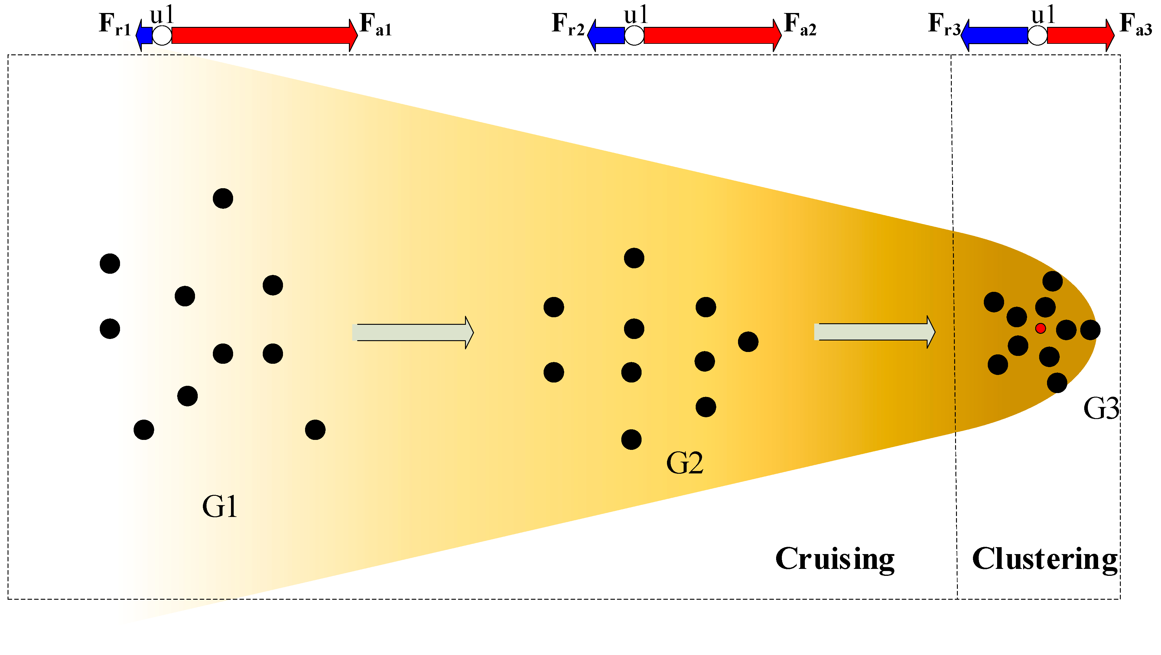
Figure 1 shows a diagram of the example scenario controlling the UAV to cruise and cluster. At the initial moment, the UAV cluster is in a dispersed state. Assume that topology G1 is formed, UAV1 is one of the UAVs, and red dot O is the target node of the cluster. According to the virtual force model, O is attractive to G1 cluster, UAV1 is attractive to O as Fa1, and UAV1 receives repulsive forces from other UAVs in the cluster as $F_{r1}={\displaystyle \sum _{i\in G1,i\ne u\mathrm{av}1}{F}_{r1i}}$. When G1 cruises close to the target point O, the formation of G1 becomes more compact, thus forming the formation topology G2. Currently, the attractive force received by UAV1 becomes Fa2, and the repulsive force received by UAV1 is Fr2. When G2 gathers into a compact cluster of spheres at the target point, forming the static topology G3, the attractive force Fa3 of UAV1 is balanced by the repulsive force and Fr3. The closer the attraction of U1 is to the target point O, the smaller it is, so there is Fa1 > Fa2 > Fa3, and the repulsive force gradually increases as the cluster becomes more compact, so there is Fr1 < Fr2 < Fr3.

Proposition 1. 

Under the artificial potential field framework, UAV swarms with fixed repulsion coefficients exhibit inherent instability post-clustering. Specifically, infinitesimal disturbances induce oscillations, with outer-ring UAVs experiencing larger amplitude oscillations than inner-ring UAVs.

Proof. 

Assuming there are $N$ UAVs in the system, the present location of the UAV $i$ is denoted as $(x,y)$, and the coordinates of the target center point are $(x_p,y_p)$. The distance of the UAV relative to the target center point is expressed as:

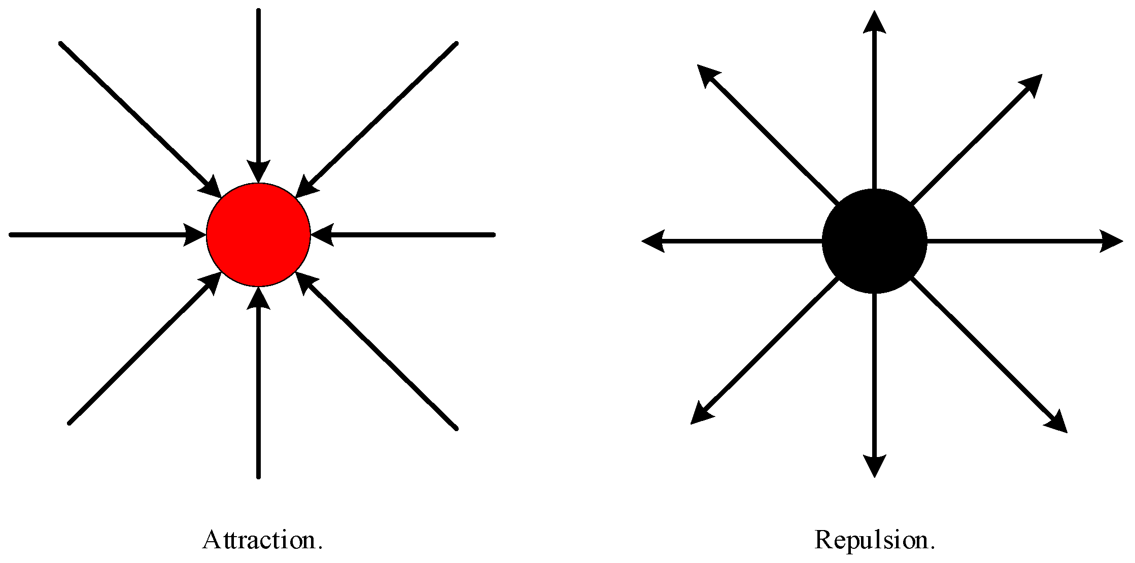
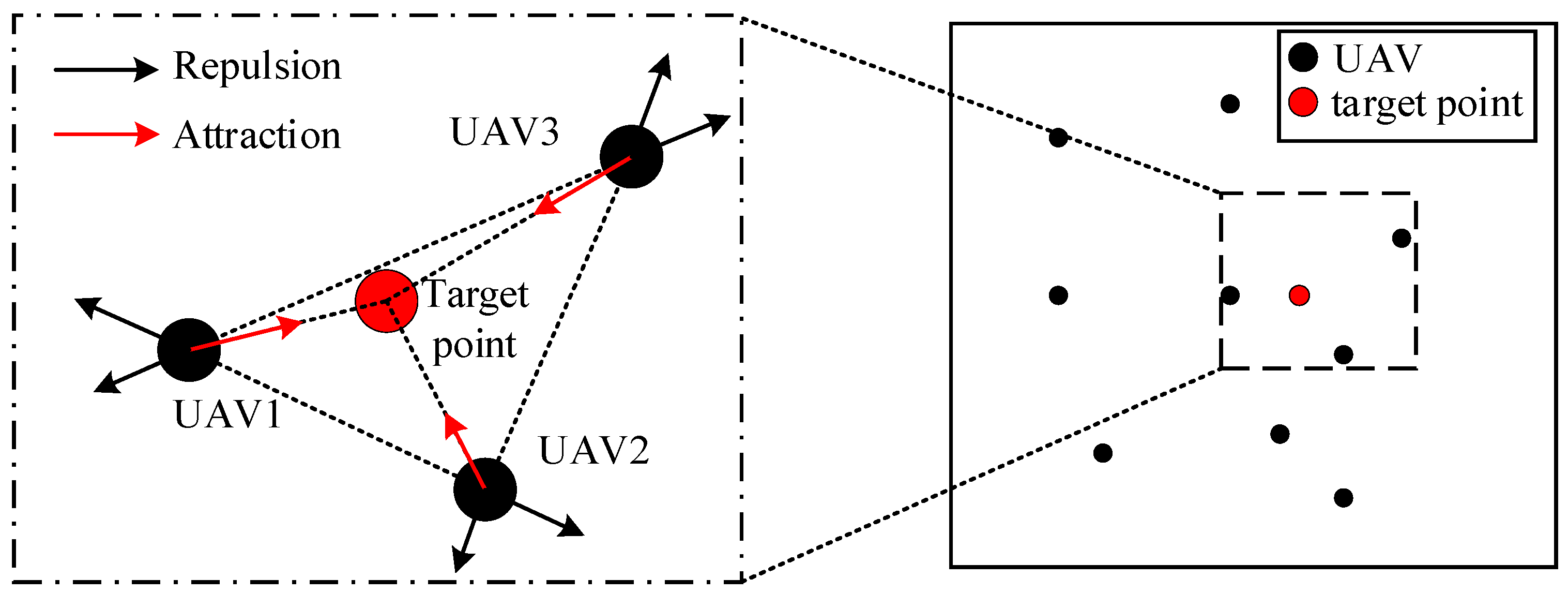
We define a target point O, which exerts an attractive force on the agent, guiding the agent toward the target point. As shown in Figure 2, the target point generates an attractive force, while the agents generate a repulsive force. Within a specific range, there is a mutual repulsive force between agents, which prevents collisions among them. The force analysis of the UAV is shown in Figure 3.

$$d_i=\sqrt{{(x_p-x)}^2+{(y_p-y)}^2}$$

(1)

The gravitational field exerted on the UAV by the target center point is defined as:

$$U_a={\displaystyle \frac{1}{2}}{k}_a{d}_i^2$$

(2)

The attraction force exerted by the target center point on the UAV is the derivative of the gravitational field:

$$F_{a,i}=k_a{d}_i{\widehat{d}}_i,$$

(3)

where $k_a$ is the attraction coefficient and ${\widehat{d}}_i$ is the unit vector pointing towards the target center point.

The repulsive field between adjacent UAVs is defined as:

$$U_r=\left\{\begin{array}{ll}{k}_b(d_{ij}^{-1}-d_0^{-1}),\hfill & d_{ij}\le d_0\hfill \\ 0,\hfill & d_{ij}>d_0\hfill \end{array},\right.$$

(4)

where $k_b$ is the repulsion coefficient, $d_{ij}$ is the relative distance between adjacent UAVs, $d_0$ is range of influence of the repulsive field.

The repulsive force is defined as:

$$F_{r,ij}=\left\{\begin{array}{ll}{k}_b{\displaystyle \frac{{\widehat{d}}_{ij}}{d_{ij}^2}},\hfill & d_{ij}\le d_0\hfill \\ 0,\hfill & d_{ij}>d_0\hfill \end{array},\right.$$

(5)

where ${\widehat{d}}_{ij}$ is the unit vector pointing about UAV $i$ to UAV $j$.

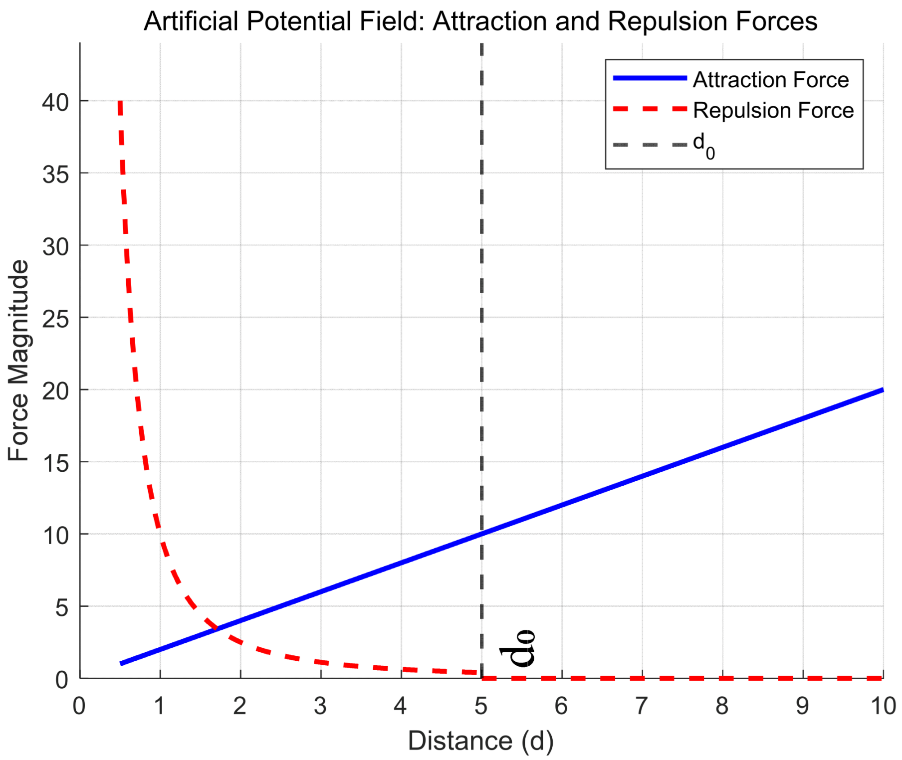
The variation of attraction and repulsion in artificial potential fields with distance is shown in Figure 4. The blue line represents attraction, which increases linearly with distance, in line with Equation (3). The red dashed line indicates repulsion, which follows an inverse-square law within the repulsion range ($d_0$). Beyond $d_0$, repulsion is zero. This also corresponds exactly to Equation (5). Parameters are set as $k_a=2$, $k_b=10$, $d_0=5$, and a minimum safe distance $d_{\min }=0.5$.

The dynamics equation of UAV $i$ is:

$$m{\ddot{x}}_i=F_{a,i}+{\displaystyle \sum _{j\ne i}^N{F}_{r,ij}}+F_{d,i}-c{\dot{x}}_i$$

(6)

In this context, ${\ddot{x}}_i$ represents the acceleration of UAV $i$, ${\displaystyle \sum _{j\ne i}^N{F}_{r,ij}}$ denotes the repulsive force from other UAVs acting on UAV $i$, $F_{d,i}$ indicates the external disturbance force applied to UAV $i$, and $c{\dot{x}}_i$ is the damping force proportional to the velocity.

Assuming a small disturbance $F_{d,i}$ is applied, the displacement $\Delta x_i$ of each UAV can be expressed as follows. The new position can be represented as:

$${x^{\prime }}_i=x_i+\Delta x_i$$

(7)

The equilibrium equation after the disturbance is:

$$\begin{array}{ll}m({\ddot{x}}_i+\Delta {\ddot{x}}_i)& =k_a(x_p-(x_i+\Delta x_i))\\ & +{\displaystyle \sum _{j\ne i}^N{k}_b\frac{(x_i+\Delta x_i)-(x_j+\Delta x_j)}{\Vert x_i+\Delta x_i-(x_j+\Delta x_j){\Vert }^2}}\\ & +F_{d,i}-c({\dot{x}}_i+\Delta {\dot{x}}_i)\end{array}$$

(8)

In the steady state before the disturbance, ${\ddot{x}}_i=0$ and ${\dot{x}}_i=0$. Therefore, the equilibrium condition is:

$$k_a(x_p-x_i)+{\displaystyle \sum _{j\ne i}^N{k}_b\frac{x_i-x_j}{\Vert x_i-x_j{\Vert }^2}}=0$$

(9)

Substituting the equilibrium conditions into Equation (8), we obtain:

$$\begin{array}{ll}m\Delta {\ddot{x}}_i+c\Delta {\dot{x}}_i& =-k_a\Delta x_i\\ & +{\displaystyle \sum _{j\ne i}^N(k_b\frac{(x_i+\Delta x_i)-(x_j+\Delta x_j)}{\Vert x_i+\Delta x_i-(x_j+\Delta x_j){\Vert }^2}-k_b\frac{x_i-x_j}{\left|\right|x_i-x_j|{|}^2}})\\ & +F_{d,i}\end{array}$$

(10)

The repulsive force term can be expanded and approximated to the first order for small disturbances.

$$\begin{array}{ll}{\displaystyle \frac{(x_i+\Delta x_i)-(x_j+\Delta x_j)}{\Vert x_i-x_j+\Delta x_i-\Delta x_j{\Vert }^2}}& \approx {\displaystyle \frac{x_i-x_j}{\Vert x_i-x_j{\Vert }^2}}+{\displaystyle \frac{\Delta x_i-\Delta x_j}{\Vert x_i-x_j{\Vert }^2}}\\ & -2{\displaystyle \frac{(x_i-x_j)\cdot (\Delta x_i-\Delta x_j)}{\Vert x_i-x_j{\Vert }^4}}(x_i-x_j)\end{array}$$

(11)

Substituting into Equation (9), we obtain:

$$\begin{array}{ll}m\Delta {\ddot{x}}_i+c\Delta {\dot{x}}_i& =-k_a\Delta x_i\\ & +{\displaystyle \sum _{j\ne i}^N(\frac{\Delta x_i-\Delta x_j}{\Vert x_i-x_j{\Vert }^2}-2\frac{(x_i-x_j)\cdot (\Delta x_i-\Delta x_j)}{\Vert x_i-x_j{\Vert }^4}(x_i-x_j))}\\ & +F_{d,i}\end{array}$$

(12)

Neglecting the second-order small quantities, the above equation can be simplified to:

$$0=-k_a\Delta x_i+{\displaystyle \sum _{j\ne i}^N{k}_b\frac{\Delta x_i-\Delta x_j}{\Vert x_i-x_j{\Vert }^2}}+F_{d,i}$$

(13)

Combining the terms involving $\Delta x_i$ and rearranging, we obtain:

$$\Delta x_i\left(k_a+{\displaystyle \sum _{j\ne i}^N\frac{k_b}{\Vert x_i-x_j{\Vert }^2}}\right)={\displaystyle \sum _{j\ne i}^N{k}_b\frac{\Delta x_j}{\Vert x_i-x_j{\Vert }^2}}+F_{d,i}$$

(14)

Thus, the displacement change for each UAV is:

$$\Delta x_i={\displaystyle \frac{k_b{\displaystyle \sum _{j\ne i}^N\frac{\Delta x_j}{\Vert x_i-x_j{\Vert }^2}}+F_{d,i}}{\left(k_a+k_b{\displaystyle \sum _{j\ne i}^N\frac{1}{\Vert x_i-x_j{\Vert }^2}}\right)}}$$

(15)

Since $\left|\right|x_p-x_j\left|\right|<\left|\right|x_q-x_j\left|\right|$:

$${\displaystyle \frac{1}{k_a+k_b{\displaystyle \sum _{j\ne i}^N\frac{1}{\Vert x_p-x_j{\Vert }^2}}}}<{\displaystyle \frac{1}{k_a+k_b{\displaystyle \sum _{j\ne i}^N\frac{1}{\Vert x_q-x_j{\Vert }^2}}}}$$

(16)

According to Equation (15), the UAVs near the target point experience less oscillation than those farther away.

$$\Delta x_p<\Delta x_q$$

(17)

Thus, the proof is complete. □

3. Cruising Stage of UAV Swarm

3.1. Basic Principle of the Proposed Sliding Mode Controller

Sliding mode control employs discontinuous signals to force system dynamics onto a designed sliding surface, ensuring ideal behavior. It involves two phases: rapid convergence to the surface (approach) and trajectory-following motion, repeated alternately until objectives are achieved.

Consider the nonlinear system shown below:

$$\dot{x}(t)=f(x,t)+g(x,t)\zeta (t)$$

(18)

where $x\in {ℝ}^n$ represents the state variable of the sliding mode system; $\zeta (t)\in {ℝ}^m$ is the control input about the sliding mode system; f(.,.), g(.,.) are different continuous functions related to $x$.

The control inputs for the sliding mode system are devised in the following way:

$$\begin{array}{l}\zeta (t)={\left[{\zeta }_1\left(t\right),{\zeta }_2\left(t\right),\dots ,{\zeta }_m\left(t\right)\right]}^T\\ {\zeta }_i\left(t\right)=\left\{\begin{array}{ll}{\zeta }_i^{+}\left(t\right),if\hfill & s_i>0,\hfill \\ {\zeta }_i^{-}\left(t\right),if\hfill & s_i>0,\hfill \end{array}\right.i=1,2,\dots ,m\end{array}$$

(19)

where ${\zeta }_i^{+}\left(t\right)\ne {\zeta }_i^{-}\left(t\right)$;$s\in {ℝ}^m$ is a switching function. Therefore, during the sliding mode motion, the transition from the convergence phase of the system to the reciprocating motion phase on the sliding mode surface depends on the function $s$, also known as the sliding mode surface. The switching function $s$ can change the control input of the system from ${\zeta }_i^{+}\left(t\right)$ to ${\zeta }_i^{-}\left(t\right)$, thereby altering the sliding mode structure.

So, during the sliding motion, the switching function $\mathrm{s}$ helps the system transition from the convergence stage towards the sliding surface to the oscillatory motion stage on the sliding surface. The switching function $s$, or sliding surface, enables the transformation of the system’s control input from point ${\zeta }_i^{+}\left(t\right)$ to point ${\zeta }_i^{-}\left(t\right)$, thus achieving a change in the structure of the sliding mode system.

First, construct appropriate switching functions. Due to different switching functions, the dynamic quality of the system is also different. Choosing a suitable sliding surface can ensure the sliding surface is in a stable state. In current practical designs, the most commonly used sliding surface is:

$$s=ce(t)+\dot{e}(t),$$

(20)

where $ce(t)$ represents the error; $\dot{e}(t)$ represents the derivative of error, indicating the rate of change of tracking error.

Regarding the reaching law for sliding mode control, there are three traditional approaches: the constant velocity reaching law, the exponential reaching law, and the power reaching law. Taking the exponential approach law as an example, when the rate at which the system approaches the sliding surface is extremely high, the system oscillation effect is strong. If the system oscillation effect is weakened, the convergence speed decreases correspondingly, and the convergence time increases.

3.2. Design and Analysis of Novel Approach Laws

The expression of the traditional exponential approach law is given as follows:

$$\dot{s}=-\epsilon sgn(s)-ks\hspace{1em}\epsilon >0,k>0$$

(21)

Taking the exponential approach law as an example, when the system is distant from the sliding surface, both the exponential approach and the constant-speed approach contribute to controlling the system’s velocity, facilitating its convergence to the sliding surface. As the system nears it, the significance of the exponential approach diminishes to the point of being negligible, leaving only the constant-speed approach effective. Composed of a sign function and a non-zero parameter $\epsilon$, the constant-speed approach ensures that the system maintains a non-zero velocity, oscillating on the sliding surface. This analysis implies that the effectiveness of sliding mode control depends on the appropriate tuning of parameters $\epsilon$ and $k$. Larger values about $\epsilon$ and $k$ lead to a more rapid convergence rate. However, this comes at the cost of more pronounced chattering effects. Conversely, smaller values of $\epsilon$ and $k$ mitigate chattering but also decelerate convergence. Its limitations can be ascertained by computing the exponential approach law’s convergence time.

In the exponential approach law, if $s>0$, we obtain:

$${\displaystyle \frac{ds}{dt}}=-\epsilon -ks$$

(22)

The duration it takes for the system to arrive at the sliding surface is:

$${\displaystyle \int \begin{array}{l}0\\ s(0)\end{array}}{\displaystyle \frac{ds}{-\epsilon -ks}}dt$$

(23)

The resulting outcome is:

$$t_1={\displaystyle \frac{1}{k}}(\ln (s(0)+{\displaystyle \frac{\epsilon }{k}})-\ln {\displaystyle \frac{\epsilon }{k}})$$

(24)

It can be clearly observed that increasing the value of $k$ can accelerate the system’s convergence speed, but the velocity at which it reaches the sliding surface will be higher. Consequently, during the reciprocating motion phase on the sliding surface, the velocity will also be higher, leading to more significant oscillations in the system. By decreasing the value of $k$, the velocity during the reciprocating motion phase on the sliding surface can be reduced. Nevertheless, the convergence rate of the system will decrease accordingly, causing an elongation in the system’s convergence time.

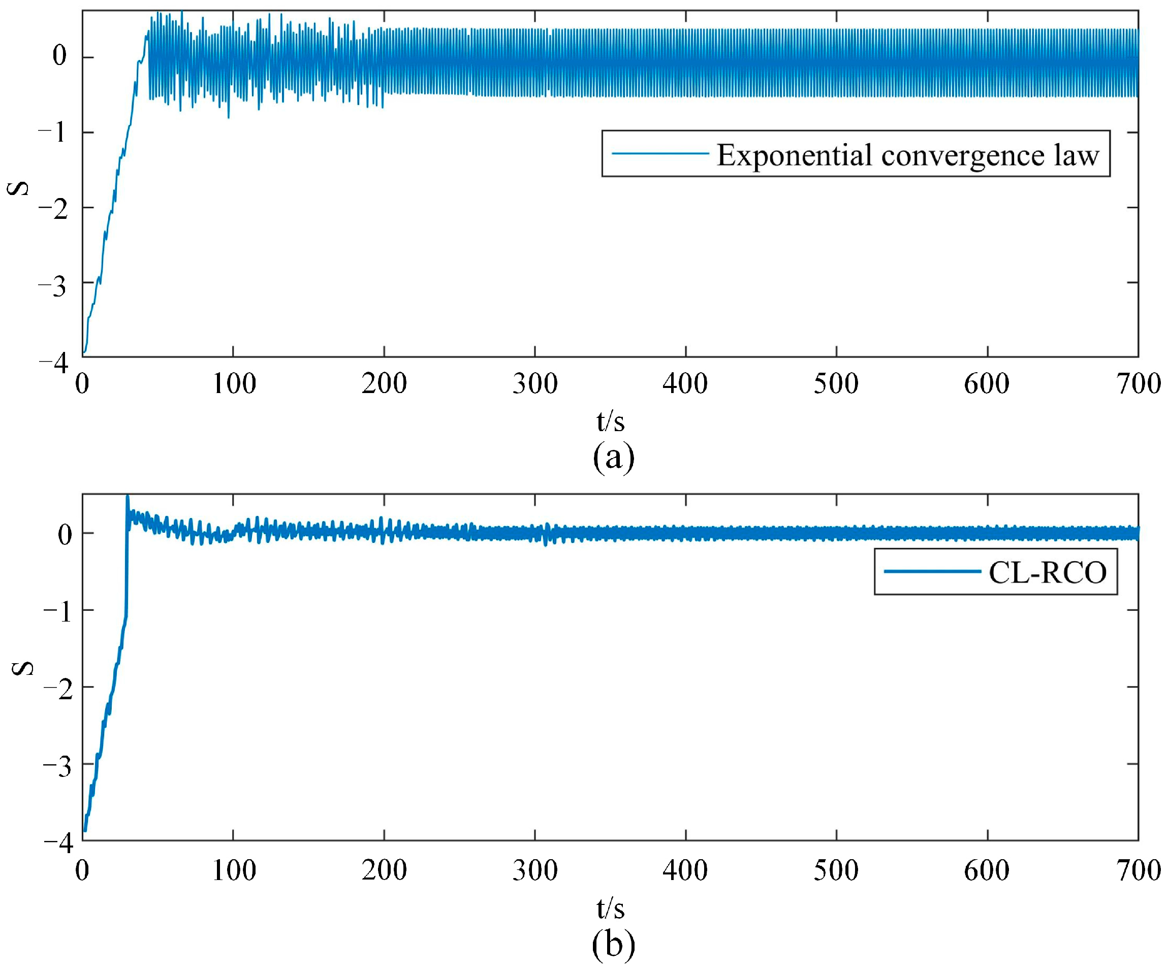
To address the limitations of the traditional exponential convergence law, the CL-RCO put forward in this paper is presented as follows:

$$\stackrel{·}{s}=-{\displaystyle \frac{k_1}{\partial e^{-\left|s\right|}+{\beta }^{\left|s\right|}}}sgn\left(s\right)-k_2{\left|s\right|}^{1-\gamma }sgn\left(s\right),$$

(25)

where $s$ is the SMC switch function, and parameters of CL-RCO satisfy $k_1,k_2>0$, $0<\partial ,\beta ,\gamma <1$.

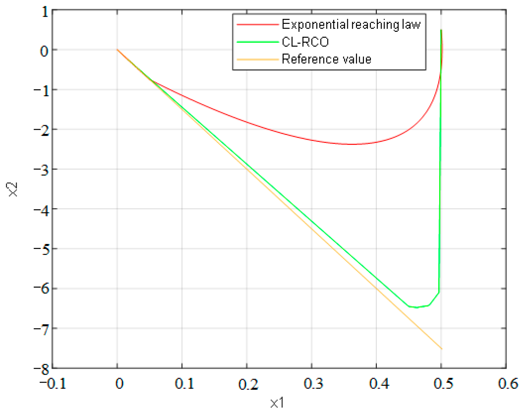
Based on theoretical analysis, the existence and feasibility of the improved exponential reaching law were verified through numerical simulation. As shown in Figure 5, where the yellow line is the reference value as the system nears the sliding surface, the exponential reaching law causes the system’s convergence speed to decelerate. However, the CL-RCO demonstrates a faster convergence speed.

3.3. Modeling UAV Swarm Cruising with CT-Control

The fundamental task of UAV formation control lies in guiding the multi-UAV system in diverse scenarios. For instance, the controller can generate diverse formations or execute varied maneuvers to maintain and reconstitute the multi-UAV formation. Thus, these control functionalities are implemented within the controller framework.

The controller initially gathers positional feedback from each UAV and issues desired position information to individual UAVs. Upon receiving the controller’s input, UAVs move towards their desired positions. Furthermore, the design of the UAV’s desired position controller does not account for the positions of neighboring UAVs. It solely guides each UAV to its intended position. Consequently, incorporating information regarding the positions of surrounding UAVs and modifying the desired positions is necessary for the UAV system to converge to an equilibrium state due to the repulsive forces exerted by neighboring agents.

To address this, once the desired-position controller of the UAV generates an output, the UAV equilibrium controller takes into account the UAV’s actual position as well as the positions of adjacent UAVs. By transforming coordinates, it computes the UAV’s desired position, enabling it to achieve motion toward the balanced formation state.

3.4. UAV Desired Position Controller

The motion state description equation of the UAV system is:

$$v_i={[\stackrel{·}{x_i} \stackrel{·}{y_i}]}^T={[v_{ix} v_{iy}]}^T$$

(26)

$${\zeta }_i={[\stackrel{·}{v_{ix}} \stackrel{·}{v_{iy}}]}^T={[{\zeta }_{ix} {\zeta }_{iy}]}^T$$

(27)

In the equation, $x_i$ and $y_i$ indicate the UAV’s horizontal and vertical positions, respectively. The velocities in the $x$- and $y$-directions are denoted by $v_{ix}$ and $v_{iy}$. Control inputs for maneuvering along these axes correspond to ${\zeta }_{ix}$ and ${\zeta }_{iy}$.

The angle of the current motion direction of the UAV is $\theta$, which can be obtained by Equation (28):

$${\theta }_i=\arctan 2(v_{iy},v_{ix})$$

(28)

The desired angle of the UAV is the angle of the line joining the current position of the UAV and the target point, i.e.,

$${\overline{\theta }}_i=\arctan 2(y_p-y,x_p-x)$$

(29)

Thus, the angular error of the UAV can be calculated by Equation (30):

$$e_i={\theta }_i-{\overline{\theta }}_i$$

(30)

Indeed, in the context of multi-UAV system control based on artificial potential fields, as it essentially revolves around virtual target tracking, the switching function formula for the sliding mode controller about the i-th UAV is presented as follows, relying on Equation (31):

$$s_i(t)=c{e}_i\left(t\right)+{\stackrel{·}{e}}_i\left(t\right)$$

(31)

In this context, $e\left(t\right)={\omega }_d(t)-\omega (t)$ signifies the disparity between the real-time location and the intended destination, while $\stackrel{·}{e}\left(t\right)=\stackrel{·}{{\omega }_{id}}(t)-\stackrel{·}{{\omega }_i}(t)$ denotes the derivative of the positional variance between the actual and intended locations, effectively capturing acceleration discrepancies. ${\omega }_{id}(t)$ encompasses the coordinates of the anticipated position for the i-th UAV at the given moment $t$. $\stackrel{··}{{\omega }_i}(t)={\zeta }_i+{\displaystyle \frac{{\displaystyle \sum _{j=1}^M{f}_i^j}}{m}}$. In this context, $\stackrel{··}{{\omega }_i}(t)$ represents the acceleration imparted by the desired target point, ${\zeta }_i$ signifies input for the i-th UAV, and ${\displaystyle \frac{{\displaystyle \sum _{j=1}^M{f}_i^j}}{m}}$ embodies the acceleration induced by repulsive forces from $m$ neighboring UAVs. The formulation can be summarized as follows:

$$\begin{array}{ll}{\stackrel{·}{s}}_i(t)& =c\stackrel{·}{e_i}\left(t\right)+{\stackrel{··}{e}}_i\left(t\right)\\ & =c(\stackrel{·}{{\omega }_{id}}(t)-{\stackrel{·}{\omega }}_i(t))+\left(\stackrel{··}{{\omega }_{id}}(t)-\stackrel{··}{{\omega }_i}(t)\right)\\ & =c(\stackrel{·}{{\omega }_{id}}(t)-\stackrel{·}{{\omega }_i}(t))+\left(\stackrel{··}{{\omega }_{id}}(t)-{\zeta }_i-{\displaystyle \frac{{\displaystyle \sum _{j=1}^M{f}_i^j}}{m}}\right)\end{array}$$

(32)

Upon substituting the CL-RCO into the current text, the resulting expression is as follows:

$$\begin{array}{l}c(\stackrel{·}{{\omega }_d}(t)-\stackrel{·}{\omega }(t))+\left(\stackrel{··}{{\omega }_d}(t)-{\zeta }_i+{\displaystyle \frac{{\displaystyle \sum _{j=1}^M{f}_i^j}}{m}}\right)\\ =-{\displaystyle \frac{k_1}{\partial e^{-\left|s\right|}+{\beta }^{\left|s\right|}}}sign\left(s\right)-k_2{\left|s\right|}^{1-\gamma }sign\left(s\right)\end{array}$$

(33)

After reorganization, the resulting expression is as follows:

$$\begin{array}{ll}\zeta (t)& =({\displaystyle \frac{k_1}{\partial e^{-\left|s\right|}+{\beta }^{\left|s\right|}}}sign(s)\\ & -k_2{\left|s\right|}^{1-\gamma }sign(s))+{\displaystyle \frac{{\displaystyle \sum _{j=1}^M{f}_i^j}}{m}}\\ & +c(\stackrel{·}{{\omega }_d}(t)-\stackrel{·}{\omega }(t))+\stackrel{··}{{\omega }_d}(t)\end{array}$$

(34)

Proposition 2. 

The cruising-stage controller integrates CL-RCO and APF, which guarantees asymptotic stability for the UAV swarm.

Proof. 

We choose a Lyapunov function as follows:

$$V_1={\displaystyle \frac{1}{2}}{s}^2$$

(35)

Take the derivative of the above equation:

$${\stackrel{·}{V}}_1=s\stackrel{·}{s}=-s{\displaystyle \frac{k_1}{\partial e^{-\left|s\right|}+{\beta }^{\left|s\right|}}}sgn\left(s\right)-s{k}_2{\left|s\right|}^{1-\gamma }sgn\left(s\right),$$

(36)

where $k_1,k_2>0$; $\partial ,\beta ,\gamma$ belong to the open interval (0, 1).

In the next step, we need to verify the system’s stability.

Given $k_1,k_2>0$,$0<\partial ,\beta ,\gamma <1$, it can be deduced with relative ease.

$$\begin{array}{l}{k}_{1}s\mathit{sgn}(s)\ge 0\\ \partial e^{-\left|s\right|}+{\beta }^{\left|s\right|}>0\\ k_{2}s{\left|s\right|}^{1-\gamma }\mathit{sgn}\left(s\right)\ge 0\end{array}$$

(37)

From the above analysis, it follows that $\stackrel{·}{V_1}\le 0$, according to the Lyapunov principle. It is known that when $\stackrel{·}{V_1}\le 0$, the system will stabilize. □

4. Clustering Stage of UAV Swarm

The exclusive reliance on UAV desired position controller outputs for motion regulation enables positional targeting but fails to maintain systemic stability. This limitation necessitates the integration of a formation balancing controller into the control architecture. The enhanced mechanism incorporates positional data from adjacent UAVs to dynamically recalibrate target coordinates, thereby enhancing positional convergence accuracy. Such a methodology effectively promotes equilibrium attainment in multi-UAV configurations through coordinated spatial adjustments.

Within the conventional artificial virtual force field approach, virtual forces of attraction and repulsion are harnessed to direct the formation of UAV swarms. The forces of attraction prompt the UAVs to converge, whereas the forces of repulsion safeguard against collisions between them. However, when using this method to form swarms, the UAVs exhibit certain levels of jitter. A segmented repulsion coefficient method has been proposed to address this issue. This method gradually decreases the repulsion coefficient as the distance between the UAVs decreases, thereby subjecting the UAVs to smoother repulsive forces and enabling them to achieve a stable state.

Simplified kinematics model for two-dimensional UAV motion:

$$\left\{\begin{array}{c}\dot{x}=u\cos \psi \\ \dot{y}=u\sin \psi \\ \dot{\psi }=\omega \end{array}\right.$$

(38)

In the model, $\psi$, $\omega$ and $u$ denote the UAV’s heading angle, angular velocity, and linear velocity, respectively. Its position is defined by the coordinates $x$ and $y$.

The UAV’s current coordinates $(x,y)$ and the target point’s position $(x_p,y_p)$ define their relative distance and angle, calculated as follows:

$$d=\sqrt{{(x_p-x)}^2+{(y_p-y)}^2}$$

(39)

$$\alpha =\mathrm{atan}(y_p-y, x_p-x)$$

(40)

Then, we define an angle error:

$$e_{\psi }=\alpha -\psi$$

(41)

By differentiating Equation (41) and then substituting the result into Equation (39), we obtain:

$$\begin{array}{ll}\dot{d}& =-{\displaystyle \frac{{\dot{y}}_c(y_p-y)+{\dot{x}}_c(x_p-x)}{d}}\\ & =-u\left(\sin (\alpha )\sin (\psi )+\cos (\alpha )\cos (\psi )\right)\\ & =-u\cos (\alpha -\psi )\end{array}$$

(42)

Upon rearrangement, we obtain:

$$\begin{array}{l}{\dot{e}}_{\psi }=\dot{\alpha }-\dot{\psi }\\ ={\displaystyle \frac{{\dot{y}}_c(y_p-y)-{\dot{x}}_c(x_p-x)}{d^2}}-\omega \\ ={\displaystyle \frac{u}{d}}\sin (e_{\psi })-\omega \end{array}$$

(43)

The artificial potential field’s attractive and repulsive forces are mathematically formulated in Equations (2)–(5). According to Equation (6), the repulsive force exerted on the UAV is large at this time. Therefore, the UAVs are prone to significant oscillations. To address this issue, a method of variable repulsion coefficient is proposed. This method dynamically adjusts the repulsion coefficient based on the distance between UAVs to smooth out the repulsive force, thereby reducing and eliminating oscillations.

Therefore, the repulsion coefficient is designed as follows:

$$k_{ib}={\displaystyle \frac{(d_i-d_{i-1})d_{i+1}}{(d_{i+1}-d_{i-1})d_i}}{k}_{(i-1)b}$$

(44)

In the division of the repulsive range, an initial safety distance $d_0$= 0.3 m is set to prevent collisions, followed by an interval of 2 m to define d1 as 2.3 m. This pattern continues with a 2 m gap between each subsequent segment, sequentially increasing the subscript of d, resulting in $d_7$= 14.3 m. With an initial repulsive coefficient $k_{0b}$= 1, the repulsive coefficients for each segment can be calculated using Equation (44).

Table 2. The repulsive coefficient for each distance segment.

d0/k0b	d1/k1b	d2/k2b	d3/k3b	d4/k4b	d5/k5b	d6/k6b	d7/k7b
0.3/0.06	2.3/0.10	4.3/0.18	6.3/0.28	8.3/0.45	10.3/0.68	12.3/0.93	14.3/1

presents the resulting repulsive coefficients. This description is formatted under standard scientific paper writing conventions.

Next is the design of the controller. First, we construct a Lyapunov function:

$$V_2={\displaystyle \frac{1}{2}}·(x^2+y^2)+U_r$$

(45)

Taking the derivative of $V$ yields:

$${\dot{V}}_2=x\cdot \dot{x}+y\cdot \dot{y}-{\displaystyle \frac{k_{ib}\cdot (x-x_0)\cdot \dot{x}+k_{ib}\cdot (y-y_0)\cdot \dot{y}}{{[{(x-x_0)}^2+{(y-y_0)}^2]}^{3/2}}}$$

(46)

After substituting Equation (38) and rearranging, we obtain:

$$\begin{array}{ll}{\dot{V}}_2& =u\cos \psi \cdot [x-{\displaystyle \frac{k_{ib}\cdot (x-x_0)}{{[{(x-x_0)}^2+{(y-y_0)}^2]}^{3/2}}}]\\ & +u\sin \psi \cdot [x-{\displaystyle \frac{k_{ib}\cdot (y-y_0)}{{[{(x-x_0)}^2+{(y-y_0)}^2]}^{3/2}}}],\end{array}$$

(47)

where we define:

$${\mathrm{x}}_s=x-{\displaystyle \frac{k_{ib}(x-x_0)}{{[{(x-x_0)}^2+{(y-y_0)}^2]}^{\frac{3}{2}}}}$$

(48)

$$y_s=y-{\displaystyle \frac{k_{ib}(y-y_0)}{{[{(x-x_0)}^2+{(y-y_0)}^2]}^{\frac{3}{2}}}}$$

(49)

Thus, Equation (47) can be simplified to:

$${\dot{V}}_2=u(x_s\cos \psi +y_s\sin \psi )$$

(50)

According to Lyapunov stability theory, $V$ and $\dot{V}$ are required. Therefore, the velocity control law $u$ is formulated through the following:

$$u=-k_u(x_s\cos \psi +y_s\sin \psi ),$$

(51)

where $k_u$ is the gain coefficient, a positive constant, and $(x_0,y_0)$ represents the centroid coordinates of all UAVs generating repulsion force on the current UAV.

Proposition 3. 

The clustering-stage controller, employing variable repulsion coefficients and backstepping control, ensures the global asymptotic stability of the UAV swarm topology.

Proof. 

The resultant expression is derived through the substitution of Equation (51) into Equation (50), yielding:

$${\stackrel{•}{V}}_2=-k_u{(x_s\cos \psi +y_s\sin \psi )}^2$$

(52)

Therefore, we can deduce that $V>0$ and $\stackrel{•}{V}\le 0$; hence, stability of the closed-loop system is rigorously guaranteed through Lyapunov’s direct method.

When the UAV is within the repulsion field, and its position is $(x_s,y_s)$, we define a new angle error $e_c={\psi }_c-\psi$, where ${\psi }_c=a\tan (y_s,x_s)$; the angle controller is designed accordingly so that the angle error tends to zero. The derivative of the angle error $e_c$ is:

$${\dot{e}}_c=({\dot{y}}_s{x}_s-y_s{\dot{x}}_s){(x_s^2+y_s^2)}^{-1}-\omega$$

(53)

Regarding the angle error, we set a Lyapunov function as:

$$V_c=e_c^2$$

(54)

Thus:

$${\dot{V}}_c=2e_c{\dot{e}}_c$$

(55)

Clearly, $V_c\ge 0$, and to ensure that $\dot{V}<0$, we set ${\dot{e}}_c=-k_c{e}_c$. The angle control law’s gain parameter $k_c$, defined as a strictly positive scalar constant, ensures satisfaction of Lyapunov’s asymptotic stability criterion. This configuration guarantees closed-loop convergence with asymptotic reduction in angular tracking error to zero.

Substituting ${\dot{e}}_c=-k_c{e}_c$ into Equation (52), we obtain the angle control law:

$$\omega =({\dot{y}}_s{x}_s-y_s{\dot{x}}_s){(x_s^2+y_s^2)}^{-1}+k_c{e}_c$$

(56)

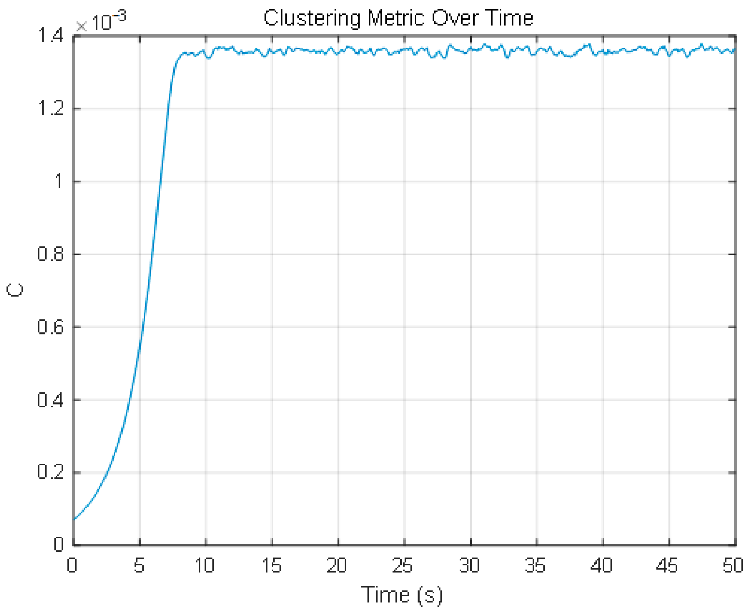
To measure the cohesion and compactness of UAV distribution, we define a quantity called clustering metric $C$.The main idea is to calculate the distance between each pair of UAVs in the UAV cluster. Sum up all these distances to obtain the total distance. The cohesion is then defined as the reciprocal of the total distance. The specific calculation method for $C$ is as follows:

Assuming that the positions of the UAVs are represented by coordinates $(x_1,y_1),(x_2,y_2),\dots ,(x_n,y_n)$, the distance can be calculated using Equation (57):

$$D={\displaystyle \sum _{i=1}^{n-1}{\displaystyle \sum _{j=i+1}^n\sqrt{{(x_i-x_j)}^2+{(y_i-y_j)}^2}}}$$

(57)

Then, the clustering metric $C$ is given by:

$$C={\displaystyle \frac{1}{D}}$$

(58)

□

5. Simulation Experiment Analysis

5.1. Simulation Analysis of the Cruising Stage of UAV Swarm

Numerical simulations of UAV formation dynamics are performed to validate the effectiveness of the developed sliding mode formation control architecture.

The parameter settings of the CL-RCO are shown in

Table 3. The parameter settings of the CL-RCO.

Parameter	CL-RCO
$k_1$	2.36945
$k_1$	21.24895
$\partial$	0.49231
$\beta$	0.00846
$\gamma$	0.12619

.

Utilizing the multi-UAV cluster aggregation process from Figure 6, the formation motion of multiple UAVs was experimentally analyzed. The simulation scenario takes place in a flat area measuring 50 m × 50 m. The set number of UAVs is 25, and the communication distance is 75 m. Under ideal communication conditions, each UAV can send and receive messages without obstruction. Since the UAVs in the same layer have similar motion characteristics during the topology formation by the cluster formation, we select one UAV in each layer for data recording, i.e., UAV1, UAV9, UAV17, and UAV25. We have simulated and recorded the angular error and the tracking error of the UAVs, where the angular error is the difference between the current angle and the desired angle of the UAV. The tracking error is the difference between the desired position and the current position.

To demonstrate the effectiveness of the CL-RCO method proposed in this paper, we have made a comparative simulation of CL-RCO with the traditional exponential convergence law.

At the beginning, the positions of all UAVs randomly appear in an area of 50 m × 50 m, after which the UAV swarms gradually converge to form a topology using the CL-RCO controller, as well as in the presence of an artificial potential field, the process of which is shown in Figure 6. Simulations in Figure 7 and Figure 8 give the output data, such as tracking distance errors and tracking angle errors.

The angular errors of UAV1, UAV9, UAV17, and UAV 25 are shown in Figure 7. It can be observed from Figure 7 that the methods using CL-RCO all exhibit relatively small angle errors compared to the exponential convergence law method. Comparing UAV1, UAV9, UAV17, and UAV25, it can be learned that the closer the UAV is to the outer circle, the more significant the error. This is because the UAVs closer to the outer circle are subjected to less force, which makes it difficult for them to reach force equilibrium, which corresponds to Proposition 1. When the UAV25 is close to the target point, it is less sensitive to the gravitational effect and the influence of the surrounding UAVs. When the UAV25 is close to the target point, it is more sensitive to gravitational effects and to the influence of surrounding UAVs, and therefore, experiences slight oscillations.

As shown in Figure 8, the tracking distance errors of UAV1, UAV9, UAV17, and UAV25 are shown, respectively. It can be observed from Figure 8 that all the methods using CL-RCO exhibit relatively small tracking distance errors compared to the exponential convergent law method. The error almost disappears as the UAV approaches the target point, resulting in stable UAV behavior. Figure 8b,d show the tracking distance error for UAV9 and UAV25, respectively. Similar to UAV9, UAV25 also exhibits a relatively small tracking distance error. However, for UAV1, the error is slightly larger. The results are because UAV1 is located at the edge of the multi-UAV cluster.

It is significant to note the convergence of angular errors in the multi-UAV system. Initially, the UAVs in the outer ring (e.g., UAV1) exhibit larger angular errors and more severe oscillations. However, under the influence of the sliding mode controller, these errors gradually converge over time. This observation validates the effectiveness of the proposed control law, as it demonstrates the system’s ability to self-correct and stabilize as the UAVs approach the target center.

The CL-RCO, as depicted in Figure 9, is crucial in controlling the oscillatory behavior of the system’s sliding surface. When both the exponential convergence law and the CL-RCO are applied as control inputs to the UAV system’s formation sliding mode controller, the system’s sliding surface exhibits a controlled oscillatory behavior. This deeper understanding of the control system’s operation enhances our comprehension of the system’s stability and convergence.

Due to the influence of the artificial potential field, the drone in motion to avoid collision has repulsive forces at play, leading to the cruising process. The state of the drone will not remain unchanged and smooth, so in the next cluster phase, we designed the controller to make the drone cluster remain stable.

5.2. Simulation Analysis of the Clustering Stage of UAV Swarm

The simulations in this section include the following. 1. Balancing the position of the UAV solely through the gravitational and repulsive fields, resulting in a topological configuration with inherent oscillations. 2. Using the controller designed in Section 4, based on a segmented repulsion coefficient, to balance the position of the UAV and achieve a topology without oscillations. Additionally, a simulation analysis was conducted on the aggregation index $C$, as defined at the end of Section 4. To highlight the effectiveness of our design method, we compare our experimental results with the traditional artificial potential field as well as the backstepping control method with fixed coefficients.

Upon comparing Figure 10, Figure 11 and Figure 12, it is evident that merely utilizing gravitational and repulsive fields to control the topology of UAV swarms without controllers leads to instability, with each UAV experiencing significant velocity fluctuations. Employing controllers stabilizes the swarm. Among these, controllers designed with a segmented repulsion coefficient outperform those with a fixed coefficient. The former enables the swarm to stabilize in a relatively shorter period, approximately 3 s, whereas the latter requires more than 5 s to achieve stability.

Subsequently, a comparative simulation of angle errors is conducted. By examining the angle errors in Figure 13, Figure 14 and Figure 15, it can be observed that during the clustering phase, without the controller, the UAV’s angle oscillates continuously within the closed interval $[-\pi , \pi ]$. However, after implementing the controller designed in this study, the UAV’s angle stabilizes as its velocity reaches a steady state. Among these controllers, the performance of the one based on a fixed repulsion coefficient is weaker than that based on a smoothed repulsion coefficient. This is mainly manifested in the fact that the controller based on a smoothed repulsion coefficient can zero the angle error in a shorter period of time.

Finally, regarding the aggregation of the drone swarm, we defined an aggregation index for analysis. Figure 16, Figure 17 and Figure 18 illustrate that the drone swarm gradually aggregates over time in all three scenarios. However, the drone swarm is highly unstable without a controller, which corresponds to this section’s first two experiments. The outcome indicates that employing a controller based on a smoothed repulsion coefficient can significantly enhance the UAV swarm’s aggregation level.

6. Conclusions

A two-stage multi-UAV formation strategy based on artificial potential fields is proposed. In the cruising phase, UAVs move from random positions toward the target point, forming a spherical topology. To enhance effectiveness, we integrate sliding mode control (SMC) with artificial potential fields and propose a novel sliding mode reaching law that not only addresses the chattering problem but also achieves faster convergence compared to traditional reaching laws (e.g., exponential reaching law). Simulations validate that the proposed law reduces chattering amplitude by approximately 40% while maintaining stability. In the clustering phase, a smooth repulsive field is designed by segmenting and smoothing the repulsion coefficient, effectively eliminating oscillations and enabling stable topology formation. Notably, our formation stability controller outperforms conventional fixed-coefficient methods by achieving oscillation-free clustering within a shorter settling time. The Lyapunov stability analysis rigorously proves the controller’s stability, and comparisons with existing artificial potential field methods demonstrate that our method is superior. Together, these results demonstrate that the proposed SMC potential field framework not only ensures stability, but also has excellent results in formation accuracy, convergence speed, and oscillation suppression of UAV swarms.