Distributed Event-Triggered-Based Adaptive Formation Tracking Control for Multi-UAV Systems Under Fixed and Switched Topologies

Abstract

This paper investigates the time-varying formation-tracking (TVFT) problem for multi-UAV systems (MUSs), where the followers need to achieve a predefined time-varying formation configuration while tracking the leader’s state. In order to reduce the consumption of communication resources, an adaptive event-triggered mechanism (AETM) is designed. By combining the advantages of the adaptive technique and the event-triggered mechanism (ETM), UAVs can realize intermittent communication without relying on global information. Secondly, to improve the flexibility of formation-tracking trajectories, the TVFT consensus protocol with non-zero leader inputs is constructed. Meanwhile, the scope of the formation-tracking feasibility condition is extended. Then, the stability of the system is verified by Lyapunov stability theory, and sufficient conditions for MUSs to realize the desired TVFT configuration are obtained. In addition, the designed consensus protocol can be applied to both fixed topologies and switching topologies. Finally, the validity of the designed algorithm is confirmed by numerical examples and software-in-the-loop (SIL) simulation experiments.

1. Introduction

Recently, the formation control of MUSs has achieved rich results [1,2,3]. Owing to its potential applications in plant protection [4] and power detection [5], formation control has emerged as a significant subfield within the collaborative control of MUSs. Formation control refers to multiple UAVs forming a specific structure to complete a predetermined task according to a preset geometry and relative positions [6,7].

As classical formation control approaches, leader-following, behavior-based, and virtual structures have been widely used in [8,9,10]. Nevertheless, these strategies have some limitations [11]. To address these limitations, consensus-based formation control schemes have emerged as a promising option [12]. Ren et al. [13] revealed that three classical formation methods are a special case in the consensus-based framework. The formation configurations of UAVs based on consensus strategies can be categorized into time-invariant formation and time-varying formation (TVF). Owing to its superior dynamic performance, TVF control has gained broader applications in engineering [14,15,16,17]. Dong et al. [18] examined the distributed TVF control based on a consensus strategy and presented a comprehensive research framework. Wang et al. [19,20] investigated the stability of time-varying formation under switching topologies. In addition, the problem of UAV formation tracking with input saturation was discussed in [21]. It should be noted that in [18,20,22], only the TVF control was considered. In practical applications, the establishment of a time-varying formation merely constitutes the initial step of the task. For instance, in a target-encirclement mission [23], the follower UAVs are required to sustain a time-varying circular formation to encircle the target UAV. In this case, the time-varying formation-tracking (TVFT) problem arises, that is, followers need to maintain time-varying formation motion while tracking the leader’s trajectory. It is important to note that the TVFT problem’s integration of leader information presents new difficulties for controller design and system stability analysis. Simultaneously, the formation-tracking feasibility condition also demands redesign. Thus, the TVFT problem of MUSs still has great research potential and exploration space.

It should be noted that the work mentioned above requires continuous information interaction among UAVs, which is disadvantageous for systems with limited computational bandwidth in [24,25]. Consequently, some scholars have explored the utilization of intermittent communication mechanisms to circumvent this shortcoming Recently, the ETM has garnered significant attention due to its superior performance [26,27,28,29,30]. Ding et al. [28] constructed an ETM-based controller for UAV formation control. Moreover, the TVFT control problem was investigated using an event-triggered strategy in [29,30]. Therefore, the introduction of ETM can significantly reduce communication redundancy. However, a common limitation of these works is the reliance on global information, that is, the minimum eigenvalue of the interaction topology. It is well known that obtaining global information not only requires high computing power of the system but also does not represent a fully distributed control strategy [31]. To further reduce the dependence on global information, the adaptive technique becomes a promising candidate. These techniques can dynamically adjust control parameters in real-time based on the system state and interactions with neighboring UAVs, which shows great flexibility and robustness. Thus, researchers have integrated the advantages of adaptive techniques and distributed ETMs, and designed the AETM [32,33,34,35,36]. The average trajectory control based on an adaptive ETM was developed in [32]. This mechanism reduces the agents’ dependence on global information while alleviating the communication load. It should be noted that many formation control problems [32,33,34] are studied under the assumption of fixed topologies. In reality, the presence of external interference may cause the communication topology to change [37]. For instance, avoiding obstacles by disconnecting the link may be necessary for formation-tracking tasks. Under such circumstances, designing an adaptive formation-tracking consensus protocol for switching topologies becomes particularly crucial [38,39,40]. Despite the substantial progress achieved in the formation problem of MUSs under switching topologies, the fully distributed formation-tracking control implemented through the AETM remains to be comprehensively explored. Consequently, constructing a TVFT consensus protocol via the AETM under switching topology represents both promising and challenging research work.

In previous research work [29,30,35], formation control without a leader or with zero leader input has been investigated. Under the formation-tracking task scenario, followers are required not only to complete formation tasks but also to follow the leader’s trajectory. Therefore, considering the leader’s control inputs is of great significance for adjusting the formation’s trajectory to avoid obstacles or complete a preset formation task. Unlike the leader–follower strategy that presets the leader’s trajectory, this paper considers the leader’s control inputs. In recent years, formation-tracking control with non-zero leader input has been addressed in [23,41], and this control method requires continuous communication between UAVs. In addition, the fully distributed formation-tracking control problem with non-zero leader input was discussed in [42,43,44,45] under fixed topologies. To our knowledge, formation-tracking control of MUSs with non-zero leader input based on AETM under switching topologies has not been reported. Therefore, this paper aims to fill this gap.

Inspired by the aforementioned research work, this paper integrates adaptive techniques and ETM to further investigate the TVFT problem of MUSs with non-zero leader inputs. Moreover, the main results are generalized to switching topologies. To the best of our knowledge, the AETM strategy has not been applied to the TVFT problem of MUSs with non-zero leader inputs. In light of this research gap, this paper designs a fully distributed TVFT consensus protocol based on AETM, which applies to both fixed and switched topologies. One of the primary challenges in this work is to construct an adaptive event-triggered scheme that is independent of the global state. Meanwhile, the formation-tracking feasibility conditions for non-zero leader inputs also need to be extended. In addition, changes in the topological structure make it difficult to analyze the system’s stability and eliminate the Zeno phenomenon. Unlike previous work [41,43,44,45] that relied on numerical simulations, this paper conducts SIL experiments to further validate the effectiveness of the algorithm. The main contributions of this paper are summarized as follows.

(1) An AETM is designed for the formation-tracking problem, which not only avoids the use of global information but also effectively reduces the occupation of communication bandwidth. Compared with using a single adaptive technique or ETM in [38,46], integrating these two strategies effectively accelerates the convergence of formation tracking. Moreover, the related results are further extended to switching topologies.

(2) A fully distributed formation-tracking consensus protocol for non-zero leader inputs is constructed. Compared with the cases in [29,30] with no leader or zero leader inputs, the flexibility of the formation trajectory is increased by considering the leader input. Furthermore, the formation-tracking feasibility conditions are extended.

(3) Sufficient criteria for achieving UAV formation-tracking configurations are obtained. The SIL simulation experiments are conducted, which further validate the effectiveness of the formation-tracking algorithm at the software level.

The overall framework of this paper is presented as follows. In Section 2, the preliminaries and the problem formulation are introduced. In Section 3, formation-tracking consensus protocols based on AETM under fixed topology and switching topology are designed, respectively. Additionally, the Zeno phenomenon in both cases is ruled out. In Section 4, some numerical examples and SIL simulation experiments are provided. Finally, the conclusion of this paper and future research directions are presented in Section 5.

2. Preliminaries and Problem Formulation

This section presents preliminary information, including notation and preparatory knowledge. Additionally, the dynamics model of the UAV and the TVFT problem are introduced.

2.1. Notations and Preparatory Knowledge

All symbols are standardized in this work. ${\lambda }_{min}\left(\mathit{𝓧}\right)$ denotes the minimum eigenvalues of matrix $\mathit{𝓧}$. ${\mathit{𝓧}}^T$ represents the transpose of matrix $\mathit{𝓧}$. $dig\{\dots \}$ denotes a diagonal matrix, $\parallel \blacksquare \parallel$ represents the Euclidean norm of vectors. ⊗ represents the Kronecker product. Note that if the dimension of a matrix is not specified, it is assumed to have the appropriate dimension for algebraic operations.

Consider the interactive topological network of MUSs composed of N UAVs as a weighted undirected graph $\mathcal{G}=(V,א,𝓦)$, where V represents the set of nodes, $א=\left\{(v_i,v_j)\right|v_i,v_j\in V\}$ denotes the set of edges, and $𝓦={\left[w_{ij}\right]}_{N\times N}$ is the weight connectivity matrix of the graph $\mathcal{G}$. $(j,i)\in א\left(t\right)$ indicates that UAVs i and j can communicate with each other, otherwise $(j,i)\notin א\left(t\right)$. In addition, $\mathcal{G}$ is undirected if and only if $(v_i,v_j)\iff (v_j,v_i)$, and $w_{ij}=w_{ji}$. If $(j,i)\in א\left(t\right)$, this indicates the existence of a link between UAV i and j. The graph $\mathcal{G}$ is considered connected if a path exists between any pair of its nodes. When $(j,i)\in א\left(t\right)$, $w_{ij}>0$, otherwise $w_{ij}=0$. $𝓓=dig\{d_1,d_2,\dots ,d_N\}$ denotes the diagonal matrix of $\mathcal{G}$ with $d_i={\sum }_{j=1,j\ne i}^N{w}_{ij}$. The Laplacian matrix is defined as $\mathcal{L}=𝓓-𝓦=\left[{\mathcal{L}}_{ij}\right]$.

Lemma 1.

(Work of [35]) If the interactive topology $\mathcal{G}$ is undirected and connected, then there exists a symmetric positive definite matrix $\mathcal{M}$ such that $\mathcal{M}=\mathcal{L}+𝓓$.

Lemma 2.

(Work of [38]) For any positive definite matrix ${\mathit{Q}}_1\in {\mathbb{R}}^{n\times n}$, there exists a symmetric matrix ${\mathit{Q}}_2\in {\mathbb{R}}^{n\times n}$ that satisfies the following inequality

$${\mathit{x}}^T\left(t\right){\mathit{Q}}_2\mathit{x}\mathbf{\left(}\mathit{t}\mathbf{\right)}\le {\lambda }_{max}\left({\mathit{Q}}_1^{-1}{\mathit{Q}}_2\right){\mathit{x}}^T\left(t\right){\mathit{Q}}_1\mathit{x}\left(t\right).$$

Assumption 1.

([35]) The matrix pair $(\mathit{A},\mathit{B})$ is stabilizable and the interactive topology is connected.

2.2. Dynamic Model of UAVs

Consider the MUSs with N follower UAVs and one leader UAV. Inspired by reference [23], the dynamic equations of the follower UAVs are simplified as follows

$$\begin{array}{c}\hfill {\dot{\mathit{x}}}_i\left(t\right)=\mathit{A}{\mathit{x}}_i\left(t\right)+\mathit{B}{\mathit{u}}_i\left(t\right),\end{array}$$

(1)

where $i=1,2,\dots ,N$, $\mathit{A}$ and $\mathit{B}$ are constant matrices, ${\mathit{x}}_i\left(t\right)$ denotes the state matrix (i.e., position information) of UAV i, and ${\mathit{u}}_i\left(t\right)$ denotes the control input matrix of UAV i as determined by the consensus protocol Equation (5). Specific details are provided in the experimental section. In addition, the formation reference trajectory is produced by the leader, and its dynamic equation is as follows

$$\begin{array}{c}\hfill \dot{\mathit{q}}\left(t\right)=\mathit{A}\mathit{q}\left(t\right)+\mathit{B}{\mathit{u}}_q\left(t\right),\end{array}$$

where $\mathit{q}\left(t\right)$ and ${\mathit{u}}_q\left(t\right)$ represent the state (i.e., position information) and control input information of leader UAV. It is important to note that in the formation-tracking task, the leader UAV generates a formation reference trajectory, which the follower UAVs are required to track. In the absence of a leader, the formation-tracking problem is equivalent to the formation control problem.

Definition 1.

(Non-zero leader input [42]) ${\mathit{u}}_{\mathit{q}}\left(t\right)$ represents the leader input and satisfies $\parallel {\mathit{u}}_q\left(t\right)\parallel \le {\mu }^{*}$, where ${\mu }^{*}>0$.

Remark 1.

Compared to leaderless formation tasks in [30,36], the formation-tracking tasks addressed in this paper are more general. Specifically, the introduction of the leader’s input requires that followers not only complete specific formation tasks but also track the leader’s trajectory. If the leader adjusts the trajectory in response to changes in the environment or mission requirements, the follower’s formation will also change. Consequently, the leader’s information is taken into account, which can enhance the flexibility of formation-tracking trajectories.

Remark 2.

Note that in [35,39], the leader is not influenced by external control inputs. This indicates that the leader’s path is entirely determined by its own dynamic characteristics and initial state. Compared with the research of [35,39], this paper discusses a more general situation, that is, the leader’s input is non-zero.

Remark 3.

This paper focuses on the theoretical framework design and numerical experiments of formation tracking. Therefore, actuator constraints and physical dynamic constraints are not involved, that is, the UAV is assumed to have perfect control authority. However, these factors are inevitable in the actual unmanned system. Especially, the complex maneuvering behavior for special environments puts high demands on the system model. Therefore, future research will incorporate actuator constraints and control saturation into the proposed framework.

2.3. Problem Formulation

The research objective of this paper is to address the multi-UAV formation-tracking problem, where all the follower UAVs need to obtain the desired formation trajectory while tracking the leader state, as illustrated in Figure 1. Figure 1 depicts a scenario with five follower UAVs and one leader UAV, where the followers track the leader’s trajectory while maintaining a time-varying formation. The definitions of the TVFT and the formation-tracking feasibility condition are presented as follows.

Definition 2.

( TVFT [19]) Let ${\mathit{\delta }}_{\mathit{i}}\left(\mathit{t}\right)$ be a piecewise continuous function. The system is said to realize the desired formation-tracking configuration if for any bounded initial state satisfying

$$\underset{t\to \infty }{lim}\parallel {\mathit{x}}_i\left(t\right)-{\mathit{\delta }}_i\left(t\right)-\mathit{q}\left(t\right)\parallel =0,i=1,2,\dots N,$$

(2)

where ${\mathit{\delta }}_i\left(t\right)$ represents the formation reference function, $\mathit{q}\left(t\right)$ is the leader state.

Definition 3.

(Formation tracking feasibility condition [44]) For each UAV i, the MUSs satisfy the conditions for realizing the TVFT configuration if $\mathit{A}{\mathit{\delta }}_i\left(t\right)-{\dot{\mathit{\delta }}}_i\left(t\right)+\mathit{B}({\mathbf{\Theta }}_i\left(t\right)-{\mathit{u}}_{\mathit{q}}\left(t\right))=0$, where ${\mathbf{\Theta }}_i\left(t\right)$ is the compensation input.

Remark 4.

In light of Definition 2, it is easy to observe that (2) can be reformulated as ${lim}_{t\to \infty }({\mathit{x}}_{\mathit{i}}\left(t\right)-{\mathit{\delta }}_i\left(t\right))-({\mathit{x}}_j\left(t\right)-{\mathit{\delta }}_j\left(t\right))=0$. The TVFT control is equivalent to the consensus structure when $\mathit{q}\left(t\right)=0$. Thus, the consensus is a particular case under the TVFT structure [17,18]. Definition 3 indicates that the formation-tracking feasibility condition is utilized to determine whether the desired formation tracking can be realized.

Definition 4.

( Zeno phenomenon [39]) If the triggering interval $[t_k^i,t_{k+1}^i)$ has a positive lower bound, that is, $t_{k+1}^i-t_k^i>{\tau }^{*}$, where ${\tau }^{*}$ denotes a positive constant. Then it can be claimed that the Zeno phenomenon of the system is ruled out.

This research aims to develop a suitable distributed adaptive formation controller that enables all UAVs to achieve the desired TVFT configuration. Consequently, this study focuses on addressing the following two key issues:

(1) What are the feasibility conditions for achieving TVFT configurations in MUSs with non-zero leader input?

(2) How can we design a fully distributed formation-tracking control strategy using AETM to achieve TVFT configurations with minimal communication resources under both fixed and switching topologies?

3. Main Results

Firstly, a fully distributed AETM is constructed for MUSs with non-zero leader inputs under fixed topologies. Meanwhile, by means of Lyapunov theory, sufficient conditions for system stability are derived. Moreover, the consensus protocol is generalized to switching topologies.

3.1. Adaptive Event-Triggered TVFT Control Under Fixed Topology

In [23], a continuous formation-tracking consensus protocol based on the states of neighboring agents is presented as follows

$${\mathit{u}}_i=𝓚\sum _{j=2}^N{w}_{ij}(({\mathit{x}}_i-{\mathit{\delta }}_i)-({\mathit{x}}_j-{\mathit{\delta }}_j))+𝓚 b_i({\mathit{x}}_i-{\mathit{\delta }}_i-\mathit{q}),$$

(3)

where $𝓚$ is the gain matrix, $b_i=1$ if the follower is connected to the leader, otherwise $b_i=0$. It can be observed that continuous communication is needed between the agents. Thus, to reduce communication resource consumption, a fully distributed formation-tracking consensus protocol based on AETM is designed. By integrating adaptive technology and ETM, UAVs can achieve friendly intermittent communication. The overall framework of the AETM is shown in Figure 2.

The time sequence of information broadcast by the i-th UAV is $\{t_0^i,t_1^i,\cdots ,t_k^i,\cdots \}$. The state transmission information at the k-th triggering instant is ${\tilde{\mathit{x}}}_i=e^{\mathit{A}(t-t_k^i)}{\mathit{x}}_i\left(t_k^i\right)$ for $t\in [t_k^i,t_{k+1}^i)$. In other words, ${\tilde{\mathit{x}}}_i$ denotes the estimation of state ${\mathit{x}}_i$ at time $t_k^i$. The measurement error of the i-th UAV is constructed as

$${\mathit{e}}_i={\tilde{\mathit{x}}}_i-{\mathit{x}}_i,$$

(4)

where $i=1,2,\dots ,N$.

In contrast to (3), a fully distributed formation-tracking consensus protocol is constructed, which can be formulated as

$$\begin{array}{cc}\hfill & {\mathit{u}}_i={𝒦}_1{x}_i+{𝒦}_2[\sum _{j\in {\mathcal{N}}_i}{d}_{ij}{w}_{ij}{\mathbf{\xi }}_i+d_{i0}{b}_i{\mathbf{\zeta }}_i]+{\mathbf{\Theta }}_i\hfill \\ \hfill & {\dot{d}}_{ij}={\gamma }_{ij}{w}_{ij}{\mathbf{\xi }}_i^T\mathbf{\Phi }{\xi }_i+{\rho }_1-d_{ij}\hfill \\ \hfill & {\dot{d}}_{i0}={\gamma }_{i0}{b}_i{\mathbf{\zeta }}_i^T\mathbf{\Phi }{\zeta }_i+{\rho }_2-d_{i0},\hfill \end{array}$$

(5)

where ${\mathbf{\xi }}_i={\tilde{\mathit{x}}}_i-{\mathit{\delta }}_i-({\tilde{\mathit{x}}}_j-{\mathit{\delta }}_j)$, ${\mathbf{\zeta }}_i={\tilde{\mathit{x}}}_i-{\mathit{\delta }}_i-\mathit{q}$, $d_{ij}$ denotes the coupling weights between followers and $d_{i0}$ denotes the weight between a follower and the leader, ${\dot{d}}_{ij}\ge 0$, ${\dot{d}}_{i0}\ge 0$ and control factors ${\gamma }_{ij}$, ${\gamma }_{i0}>0$. ${\rho }_1$ and ${\rho }_2$ are positive constants. ${\mathbf{\Theta }}_i\left(t\right)$ is the formation compensation input, which is determined by the formation function ${\mathit{\delta }}_i\left(t\right)$. ${𝒦}_1,{𝒦}_2$ and $\mathbf{\Phi }$ are the feedback matrices to be determined, respectively. It is easy to observe that all the parameters in the protocol (5) are independent of the global state information. Thus, this protocol is fully distributed. Algorithm  1 presents the design of a consensus protocol based on AETM under fixed topologies.

Algorithm 1 Design of AETM-based TVFT consensus protocol in fixed topology.

Step (I): With respect to UAV i, $j\in N_i$ and formation compensation input ${\mathbf{\Theta }}_i$, the TVFT configuration is gradually realized if the following formation-tracking feasibility condition is satisfied under protocol (5). $$(\mathit{A}+\mathit{B}{𝓚}_1){\mathit{\delta }}_i-{\dot{\mathit{\delta }}}_i+\mathit{B}({\mathbf{\Theta }}_i-{\mathit{u}}_q)=0.$$ Step (II): If Step (I) is satisfied, a positive definite matrix $𝓟$ can be obtained by solving the following inequality. $${(\mathit{A}+\mathit{B}{𝓚}_1)}^T{𝓟}^{-1}+{𝓟}^{-1}(\mathit{A}+\mathit{B}{𝓚}_1)-2{\alpha }_{*}{𝓟}^{-1}\mathit{B}{\mathit{B}}^T{𝓟}^{-1}+{\alpha }_{*}\mathit{I}<0.$$ Step (III): Choose appropriate initial values for the coupling weights $d_{ij}\left(t\right)$ and $d_{i0}\left(t\right)$. Meanwhile, the positive constants ${\rho }_1$ and ${\rho }_2$ satisfy the conditions ${\rho }_1$ and ${\rho }_2>\left(0\right)$. Step (IV): The gain matrices ${𝓚}_{\mathbf{2}}$ and $\mathbf{\Phi }$ in (5) are derived as ${𝒦}_{\mathbf{2}}=-{\mathit{B}}^{\mathit{T}}{𝓟}^{-1},\mathbf{\Phi }=𝓟\mathit{B}{\mathit{B}}^{\mathit{T}}𝓟.$ Step (V): Calculate the triggering threshold, if the triggering mechanism (6) is satisfied, reset $∥{\mathit{e}}_{\mathit{i}}\left(t\right)∥=0$. Meanwhile the i-th UAV updates the controller ${\mathit{u}}_{\mathit{i}}\left(t_{k+1}^i\right)$ and the state ${\mathit{x}}_{\mathit{i}}\left(t_{k+1}^i\right)$ for $i\in N\}$, and broadcast state information to its neighbors.

The triggering mechanism of the i-th UAV is defined as

$$\begin{array}{c}\hfill t_{k+1}^i=inf\{t>t_k^i|g_i\left(t\right)\ge 0\},\end{array}$$

(6)

where $g_i\left(t\right)$ represents the triggering function, designed as follows

$$\begin{array}{c}\hfill g_i\left(t\right)={\mathsf{\Psi }}_i-{\mathsf{{\rm Y}}}_i-{\eta }_i,\end{array}$$

(7)

in which

$$\begin{array}{cc}\hfill {\mathsf{\Psi }}_i=& \left(\sum _{j\in N_i}\left(d_{ij}+{\rho }_1\right)w_{ij}+\left(2d_{i0}-{\rho }_2\right)b_i\right){{\mathit{e}}_{\mathit{i}}}^T\mathbf{\Phi }{\mathit{e}}_i,\hfill \end{array}$$

(8)

$$\begin{array}{cc}\hfill {\mathsf{{\rm Y}}}_i=& {\sigma }^{*}\sum _{j\in N_i}\left({\rho }_1-d_{ij}\right)w_{ij}{\mathbf{\xi }}_i^T\mathbf{\Phi }{\mathbf{\xi }}_i,{\sigma }^{*}>0,\hfill \end{array}$$

(9)

where ${\eta }_i={\mu }_i{e}^{-\omega t}$, ${\mu }_i>0$, $\omega >0$. The event-triggered rule (6) ensures $g_i\left(t\right)<0$ for $t\in [t_k^i,t_{k+1}^i)$, thereby preventing unnecessary state updates. Otherwise, the i-th UAV broadcasts the state information $x_i\left(t_{k+1}^i\right)$ to its neighboring UAVs. Meanwhile, the function $g_i\left(t\right)$ is computed based on the sampling information of its neighboring UAVs.

Remark 5.

The formation-tracking feasibility condition indicates that not all formations can be realized. Therefore, the desired TVFT configuration can be achieved if and only if there exists a suitable feasible set. Note that the gain matrix ${𝓚}_1$ and $u_q$ in (10) extends the feasible set of TVFT. If ${𝓚}_1=0$, the feasibility condition in (10) is equivalent to the configuration in [44]. In addition, the feasibility condition in [45] satisfies $\mathit{A}{\mathit{\delta }}_{\mathit{i}}=\mathit{B}{\mathbf{\Theta }}_{\mathit{i}}+{\dot{\mathit{\delta }}}_i$, which is a special case of (10). Note that if ${\mathbf{\Theta }}_{\mathit{i}}=0$ and ${\mathit{\delta }}_{\mathit{i}}\left(t\right)=0$, it implies that the formation is time-invariant.

Remark 6.

In this paper, an adaptive formation-tracking consensus protocol is developed by integrating adaptive techniques and the ETM. Notably, the time-varying coupling weights $d_{ij}$ and $d_{i0}$ are incorporated into the consensus protocol and the triggering mechanism. Unlike the mechanisms in [20,35], a hybrid triggering strategy that combines state-dependent and time-dependent components (i.e., an exponential term) is proposed. The inclusion of exponential terms can significantly reduce the frequency of controller updates.

According to the consensus protocol (5), the MUSs described by Equation (1) can be rewritten as follows

$${\dot{\mathit{x}}}_i=\mathit{A}{\mathit{x}}_i+\mathit{B}{\mathit{u}}_i=(\mathit{A}+\mathit{B}{𝓚}_1){\mathit{x}}_i+\mathit{B}{\mathbf{\Theta }}_i-\mathit{B}{\mathit{B}}^T𝓟[\sum _{j\in N_i}{d}_{ij}{w}_{ij}{\mathbf{\xi }}_i+d_{i0}{b}_i{\mathbf{\zeta }}_i].$$

(10)

Let ${\mathit{\psi }}_i={\mathit{x}}_i-{\mathit{\delta }}_i-\mathit{q}$. We further obtain

$$\begin{array}{c}\hfill {\tilde{\mathit{x}}}_i-{\mathit{\delta }}_i-({\tilde{\mathit{x}}}_j-{\mathit{\delta }}_j)={\mathit{\psi }}_i-{\mathit{\psi }}_j+{\mathit{e}}_i-{\mathit{e}}_j.\end{array}$$

(11)

Thus

$$\begin{array}{cc}\hfill {\dot{\mathit{\psi }}}_i=& {\dot{\mathit{x}}}_i-{\dot{\mathit{\delta }}}_i-\dot{\mathit{q}}\hfill \\ \hfill =& (\mathit{A}+\mathit{B}{𝓚}_1)({\mathit{\psi }}_i+{\mathit{\delta }}_i)-{\dot{\mathit{\delta }}}_i-\mathit{B}({\mathit{u}}_{\mathit{q}}\left(t\right)-{\mathbf{\Theta }}_i)-\mathit{B}{\mathit{B}}^T𝓟[\sum _{j\in N_i}{d}_{ij}{w}_{ij}{\mathbf{\xi }}_i+d_{i0}{b}_i{\mathbf{\zeta }}_i\left(t\right)].\hfill \end{array}$$

(12)

The following results demonstrate that the system can achieve the desired TVFT configuration through the AETM under fixed topologies.

Theorem 1.

Consider that the MUSs satisfy Assumptions 1, and the formation vector ${\delta }_i$ in Algorithm 1 holds. The desired TVFT configuration of MUSs with non-zero leader inputs can be achieved using the distributed control protocol (5) and the AETM (6) determined in Algorithm 1 under a fixed topology. Moreover, the Zeno phenomenon is avoided for all UAVs.

Proof of Theorem 1.

The candidate Lyapunov function is presented as

$$\begin{array}{c}\hfill 𝒱=𝒱*+𝒱**,\end{array}$$

(13)

in which

$$\begin{array}{cc}\hfill & 𝒱*=\sum _{i=1}^N{\mathit{\psi }}_i^T𝓟{\mathit{\psi }}_i,\hfill \end{array}$$

(14)

$$\begin{array}{cc}\hfill & 𝒱**=\sum _{i=1}^N\sum _{j\in N_i}{\displaystyle \frac{{(d_{ij}-{\rho }_1)}^2}{2{\gamma }_{ij}}}+\sum _{i=1}^N{\displaystyle \frac{{(d_{i0}-{\rho }_2)}^2}{2{\gamma }_{i0}}},\hfill \end{array}$$

(15)

where ${\gamma }_{ij}>0$, ${\gamma }_{i0}>0,$${\rho }_1$, ${\rho }_2$ are positive constants and $𝒱$ is positive definite. The trajectory of $𝒱*$ and $𝒱**$ along (5) are computed as

$$\begin{array}{cc}\hfill & \dot{𝒱}*=2\sum _{i=1}^N{\mathit{\psi }}_i^T𝓟{\dot{\mathit{\psi }}}_i,\hfill \end{array}$$

(16)

$$\begin{array}{cc}\hfill & \dot{𝒱}**=\sum _{i=1}^N\sum _{j\in N_i}{\displaystyle \frac{(d_{ij}-{\rho }_1)}{2{\gamma }_{ij}}}{\dot{d}}_{ij}+\sum _{i=1}^N{\displaystyle \frac{(d_{i0}-{\rho }_2)}{2{\gamma }_{i0}}}{\dot{d}}_{i0}.\hfill \end{array}$$

(17)

Thus, it follows from (5), (14), and (16), we have

$$\begin{array}{cc}\hfill \dot{𝒱}*=& \sum _{i=1}^N{\mathsf{\Lambda }}_i-\sum _{i=1}^N\sum _{j\in N_i}\left[d_{ij}{w}_{ij}{({\mathit{\psi }}_i-{\mathit{\psi }}_j)}^T\mathbf{\Phi }({\mathit{\psi }}_i-{\mathit{\psi }}_j)\right]\hfill \\ \hfill & -\sum _{i=1}^N\sum _{j\in {\mathcal{N}}_i}{d}_{ij}{w}_{ij}{({\mathit{\psi }}_i-{\mathit{\psi }}_j)}^T\mathbf{\Phi }({\mathit{e}}_i-{\mathit{e}}_j)-2\sum _{i=1}^N{d}_{i0}{b}_i({\mathit{\psi }}_{i}T\mathbf{\Phi }{\mathit{\psi }}_i+{\mathit{\psi }}_{i}T\mathbf{\Phi }{\mathit{e}}_i),\hfill \end{array}$$

(18)

where ${\mathsf{\Lambda }}_i={\mathit{\psi }}_i^T[𝓟(\mathit{A}+\mathit{B}{𝓚}_1)+{(\mathit{A}+\mathit{B}{𝓚}_1)}^T𝓟]{\mathit{\psi }}_i$, $\mathbf{\Phi }=𝓟\mathit{B}{\mathit{B}}^T𝓟$. Then, applying Young’s inequality to the last term of (18), we obtain the following

$$\begin{array}{cc}\hfill \dot{𝓥}*\le & \sum _{i=1}^N{\mathsf{\Lambda }}_i-\sum _{i=1}^N\left[d_{ij}{w}_{ij}{({\mathit{\psi }}_i-{\mathit{\psi }}_j)}^T\mathbf{\Phi }({\mathit{\psi }}_i-{\mathit{\psi }}_j)\right]\hfill \\ \hfill & -\sum _{i=1}^N\sum _{j\in N_i}{d}_{ij}{w}_{ij}{({\mathit{\psi }}_i-{\mathit{\psi }}_j)}^T\mathbf{\Phi }({\mathit{e}}_i-{\mathit{e}}_j)-\sum _{i=1}^N{d}_{i0}{b}_i{\mathit{\psi }}_{i}T\mathbf{\Phi }{\mathit{\psi }}_i+\sum _{i=1}^N{d}_{i0}{b}_i{\mathit{e}}_{i}T\mathbf{\Phi }{\mathit{e}}_i.\hfill \end{array}$$

(19)

Subsequently, it can be inferred from (5) and (17) that

$$\begin{array}{cc}\hfill \dot{𝒱}**=& \sum _{i=1}^N\sum _{j\in N_i}{\displaystyle \frac{(d_{ij}-{\rho }_1)}{2}}{w}_{ij}{({\mathit{\psi }}_i-{\mathit{\psi }}_j)}^T\mathbf{\Phi }({\mathit{\psi }}_i-{\mathit{\psi }}_j)\hfill \\ \hfill & +\sum _{i=1}^N\sum _{j\in N_i}{\displaystyle \frac{(d_{ij}-{\rho }_1)}{2}}{w}_{ij}{({\mathit{e}}_i-{\mathit{e}}_j)}^T\mathbf{\Phi }({\mathit{e}}_i-{\mathit{e}}_j)\hfill \\ \hfill & +\sum _{i=1}^N\sum _{j\in N_i}(d_{ij}-{\rho }_1)w_{ij}{({\mathit{\psi }}_i-{\mathit{\psi }}_j)}^T\mathbf{\Phi }({\mathit{e}}_i-{\mathit{e}}_j)\hfill \\ \hfill & +\sum _{i=1}^N{\displaystyle \frac{(d_{i0}-{\rho }_2)}{2}}{b}_i{({\mathit{\psi }}_i+{\mathit{e}}_i)}^T\mathbf{\Phi }({\psi }_i+{\mathit{e}}_i)-\sum _{i=1}^N{\mathsf{\Xi }}_i,\hfill \end{array}$$

(20)

where ${\mathsf{\Xi }}_i={\sum }_{j\in N_i}{\displaystyle \frac{{(d_{ij}-{\rho }_1)}^2}{2}}-{\displaystyle \frac{{(d_{i0}-{\rho }_2)}^2}{2}}$. As for (20), on can obtain

$$\begin{array}{cc}\hfill & \sum _{i=1}^N{\displaystyle \frac{(d_{i0}-{\rho }_2)}{2}}{b}_i{({\mathit{\psi }}_i+{\mathit{e}}_i)}^T\mathbf{\Phi }({\mathit{\psi }}_i+{\mathit{e}}_i)\hfill \\ \hfill & \le \sum _{i=1}^N(d_{i0}-{\rho }_2)b_i{\mathit{\psi }}_i^T\mathbf{\Phi }{\mathit{\psi }}_i+\sum _{i=1}^N(d_{i0}-{\rho }_2)b_i{\mathit{e}}_i^T\mathbf{\Phi }{\mathit{e}}_i.\hfill \end{array}$$

(21)

Summarizing the above analysis and combining (19)–(21), we obtain the following

$$\begin{array}{cc}\hfill \dot{𝒱}=& 𝒱*+\dot{𝒱}**\hfill \\ \hfill \le & \sum _{i=1}^N{\mathsf{\Lambda }}_i-\sum _{i=1}^N\sum _{j\in N_i}{\displaystyle \frac{(d_{ij}+{\rho }_1)}{2}}{w}_{ij}{({\mathit{\psi }}_i-{\mathit{\psi }}_j)}^T\mathbf{\Phi }({\mathit{\psi }}_i-{\mathit{\psi }}_j)\hfill \\ \hfill & -\sum _{i=1}^N\sum _{j\in N_i}{\rho }_1{w}_{ij}{({\mathit{\psi }}_i-{\mathit{\psi }}_j)}^T\mathbf{\Phi }({\mathit{e}}_i-{\mathit{e}}_j)+\sum _{i=1}^N\sum _{j\in N_i}{\displaystyle \frac{(d_{ij}-{\rho }_1)}{2}}{w}_{ij}{({\mathit{e}}_i-{\mathit{e}}_j)}^T\mathbf{\Phi }({\mathit{e}}_i-{\mathit{e}}_j)\hfill \\ \hfill & +\sum _{i=1}^N(2d_{i0}-{\rho }_2)b_i{\mathit{e}}_{i}T\mathbf{\Phi }{\mathit{e}}_i-\sum _{i=1}^N{\rho }_2{b}_i{\mathit{\psi }}_{i}T\mathbf{\Phi }{\mathit{\psi }}_i-\sum _{i=1}^N{\mathsf{\Xi }}_i.\hfill \end{array}$$

(22)

Similarly, by applying Young’s inequality, the following equation holds

$$\begin{array}{cc}\hfill -& \sum _{i=1}^N\sum _{j\in N_i}{\rho }_1{w}_{ij}{({\mathit{\psi }}_i-{\mathit{\psi }}_j)}^T\mathbf{\Phi }({\mathit{e}}_i-{\mathit{e}}_j)\hfill \\ \hfill \le & \sum _{i=1}^N\sum _{j\in N_i}{\displaystyle \frac{{\rho }_1}{2}}{w}_{ij}{({\mathit{\psi }}_i-{\mathit{\psi }}_j)}^T\mathbf{\Phi }({\mathit{\psi }}_i-{\mathit{\psi }}_j)+\sum _{i=1}^N\sum _{j\in N_i}{\displaystyle \frac{{\rho }_1}{2}}{w}_{ij}{({\mathit{e}}_i-{\mathit{e}}_j)}^T\mathbf{\Phi }({\mathit{e}}_i-{\mathit{e}}_j).\hfill \end{array}$$

(23)

Note that the formation error can be reformulated as

$$\begin{array}{cc}\hfill {\mathit{e}}_i-{\mathit{e}}_j& ={\tilde{\mathit{x}}}_i-{\mathit{\delta }}_i-({\tilde{\mathit{x}}}_j-{\mathit{\delta }}_j)-({\mathit{\psi }}_i-{\mathit{\psi }}_j)\hfill \\ \hfill & ={\mathbf{\xi }}_i-({\mathit{\psi }}_i-{\mathit{\psi }}_j).\hfill \end{array}$$

(24)

Thus, we further have

$$\begin{array}{cc}\hfill & \sum _{i=1}^N\sum _{j\in N_i}{\displaystyle \frac{(d_{ij}-{\rho }_1)}{2}}{w}_{ij}{({\mathit{e}}_i-{\mathit{e}}_j)}^T\mathbf{\Phi }({\mathit{e}}_i-{\mathit{e}}_j)\hfill \\ \hfill =& \sum _{i=1}^N\sum _{j\in N_i}{\displaystyle \frac{(d_{ij}-{\rho }_1)}{2}}{w}_{ij}{\mathbf{\xi }}_i^T\mathbf{\Phi }{\mathbf{\xi }}_i+\sum _{i=1}^N\sum _{j\in N_i}{\displaystyle \frac{(d_{ij}-{\rho }_1)}{2}}{w}_{ij}{({\mathit{\psi }}_i-{\mathit{\psi }}_j)}^T\mathbf{\Phi }({\mathit{\psi }}_i-{\mathit{\psi }}_j)\hfill \\ \hfill & +\sum _{i=1}^N\sum _{j\in N_i}(d_{ij}-{\rho }_1)w_{ij}{\mathbf{\xi }}_i^T\mathbf{\Phi }({\mathit{e}}_i-{\mathit{e}}_j).\hfill \end{array}$$

(25)

Since $w_{ij}=w_{ji}$, by applying Young’s inequality again, we can obtain the following simplified equation

$$\begin{array}{c}\hfill \sum _{i=1}^N\sum _{j\in N_i}{w}_{ij}{({\mathit{e}}_i-{\mathit{e}}_j)}^T\mathbf{\Phi }({\mathit{e}}_i-{\mathit{e}}_j)\le 4\sum _{i=1}^N\sum _{j\in N_i}{w}_{ij}{\mathit{e}}_i^T\mathbf{\Phi }{\mathit{e}}_i.\end{array}$$

(26)

Submitting (23)–(26) to (22), one has

$$\begin{array}{cc}\hfill \dot{𝒱}\le & \sum _{i=1}^N{\mathsf{\Lambda }}_i-\sum _{i=1}^N{\mathsf{\Xi }}_i-\sum _{i=1}^N{\rho }_2{b}_i{\mathit{\psi }}_i^T\mathbf{\Phi }{\mathit{\psi }}_i-\sum _{i=1}^N\sum _{j\in N_i}{\displaystyle \frac{{\rho }_1}{2}}{w}_{ij}{({\mathit{\psi }}_i-{\mathit{\psi }}_j)}^T\mathbf{\Phi }({\mathit{\psi }}_i-{\mathit{\psi }}_j)\hfill \\ \hfill & +\sum _{i=1}^N\sum _{j\in N_i}2{\rho }_1{w}_{ij}{\mathit{e}}_i^T\mathbf{\Phi }{\mathit{e}}_i^T+\sum _{i=1}^N\sum _{j\in N_i}{\displaystyle \frac{d_{ij}-{\rho }_1}{2}}{w}_{ij}{\xi }_i^T\mathbf{\Phi }{\mathbf{\xi }}_i\hfill \\ \hfill & +2\sum _{i=1}^N\sum _{j\in N_i}(d_{ij}-{\rho }_1)w_{ij}{\mathbf{\xi }}_i^T\mathbf{\Phi }{\mathit{e}}_i+\sum _{i=1}^N(2d_{i0}-{\rho }_2)b_i{\mathit{e}}_i^T\mathbf{\Phi }{\mathit{e}}_i.\hfill \end{array}$$

(27)

For the sake of this analysis, we let ${\mathit{\psi }}^T={[{\mathit{\psi }}_1^T,{\mathit{\psi }}_2^T,\dots ,{\mathit{\psi }}_N^T]}^T$. Based on Equation (27) and Lemma 1, we can rewrite it in the form of a tight set as follows

$$\begin{array}{cc}\hfill \dot{𝒱}\le & {\mathit{\psi }}^T[I_n\otimes (𝓟(\mathit{A}+\mathit{B}{𝓚}_1)+{(\mathit{A}+\mathit{B}{𝓚}_1)}^T𝓟)-(\alpha \mathcal{L}+\beta 𝓓)\otimes \mathbf{\Phi }]\mathit{\psi }-\sum _{i=1}^N{\mathsf{\Xi }}_i\hfill \\ \hfill & +3\sum _{i=1}^N\sum _{j\in N_i}{\displaystyle \frac{\left(d_{ij}-{\rho }_1\right)}{2}}{w}_{ij}{\mathbf{\xi }}_i^T\mathbf{\Phi }{\mathbf{\xi }}_i+\sum _{i=1}^N\left[\sum _{j\in N_i}\left(d_{ij}+{\rho }_1\right)w_{ij}+\left(2d_{i0}-{\rho }_2\right)b_i\right]{\mathit{e}}_i^T\mathbf{\Phi }{\mathit{e}}_i.\hfill \end{array}$$

(28)

Considering the triggering mechanism in (6), (28) can be rewritten as

$$\begin{array}{cc}\hfill \dot{𝒱}\le & {\mathit{\psi }}^T[I_n\otimes (𝓟(\mathit{A}+\mathit{B}{𝓚}_1)+{(\mathit{A}+\mathit{B}{𝓚}_1)}^T𝓟)-(\alpha \mathcal{L}+\beta 𝓓)\otimes \mathbf{\Phi }]\mathit{\psi }\hfill \\ \hfill & +\sum _{i=1}^N{\mu }_i{e}^{-\omega t}-\sum _{i=1}^N{\mathsf{\Xi }}_i.\hfill \end{array}$$

(29)

According to Algorithm 1, by choosing appropriate values for $\kappa$, ${\rho }_1$, and ${\rho }_2$, we can conclude that

$$\begin{array}{cc}\hfill \dot{𝒱}\le & -{\displaystyle \frac{{\rho }_1{\lambda }_{min}\left(\mathcal{M}\right)}{2}}{\mathit{\psi }}_i^T{\mathit{\psi }}_i+\sum _{i=1}^N{\mu }_i{e}^{-\omega t}-\sum _{i=1}^N{\mathsf{\Xi }}_i\hfill \\ \hfill \le & -\kappa 𝓥+N\mu e^{-\omega t},\hfill \end{array}$$

(30)

where $\kappa =min\{(\left[{\rho }_1{\lambda }_{min}\left(\mathcal{M}\right)\right]/2{\lambda }_{max}\left(𝓟\right)),{\gamma }_{ij},{\gamma }_{i0}\}$. According to (30), we further have

$$\begin{array}{cc}\hfill 𝒱\left(t\right)& \le e^{-\kappa \left(t-t_0\right)}𝒱\left(t_0\right)+N{\int }_{t_0}^t{e}^{-\kappa \left(t-\tau \right)}\mu e^{-\omega \tau }{d}_{\tau }\hfill \\ & =e^{-\kappa t}𝒱\left(t_0\right)+{\displaystyle \frac{N\mu }{{\kappa }_2-{\kappa }_1}}\left(e^{-\omega \left(t-t_0\right)}-e^{-\kappa \left(t-t_0\right)}\right)\le e^{-\omega \left(t-t_0\right)}{𝒱}_0,\hfill \end{array}$$

(31)

where ${𝒱}_0\left(t_0\right)=𝒱\left(t_0\right)+(N\mu /[\kappa -\omega ])$.

Thus, based on Equation (31), we can conclude that the coupling weights and ${\psi }_i$ are bounded. Meanwhile, the system converges to the desired formation-tracking configuration at an exponential rate. The constructed Lyapunov function intuitively evaluates the stability of the dynamical system through an energy measure, predicts the system’s behavior, and verifies the effectiveness of the control strategy. By adjusting the control parameters, it is feasible to design control strategies to stabilize the system. In a multi-UAV formation-tracking scenario, if the system’s stability is proven based on the Lyapunov stability theory, the desired TVFT configuration can be realized.

In light of Theorem 1, we can observe that $𝒱\ge 0$ and $\dot{𝒱}\le 0$. Thus, the energy $𝒱$ is bounded. In this case, for the adaptive coupling weights, we derive the following

$$\begin{array}{c}\hfill \sum _{i=1}^N\sum _{j\in {\mathcal{N}}_i}{\displaystyle \frac{{(d_{ij}-{\rho }_1)}^2}{4{\gamma }_{ij}}}\le 𝒱\left(0\right),\sum _{i=1}^N{\displaystyle \frac{{(d_{i0}-{\rho }_2)}^2}{4{\gamma }_{i0}}}\le 𝒱\left(0\right).\end{array}$$

(32)

Thus, we conclude that $d_{ij}$ and $d_{i0}$ are bounded. Specifically, $\parallel d_{ij}\parallel \le \tilde{d}=2\sqrt{𝒱\left(0\right){\gamma }_{ij}}+{\rho }_1$ and $\parallel d_{i0}\left(t\right)\parallel \le \overline{d}=2\sqrt{𝒱\left(0\right){\gamma }_{i0}}+{\rho }_2$. Considering the error ${\mathit{e}}_i$ of the i-th UAV for $t\in [t_k^i,t_{k+1}^i)$, the derivative of ${\mathit{e}}_i$ is calculated as follows

$$\begin{array}{cc}\hfill {\dot{\mathit{e}}}_i=& \mathit{A}{\mathit{e}}_i-\mathit{B}{u}_i=\mathit{A}{\mathit{e}}_i-\mathit{B}{𝓚}_1{\mathit{x}}_i-\mathit{B}{\mathbf{\Theta }}_i-\mathit{B}{𝓚}_2[\sum _{j\in N_i}{d}_{ij}{w}_{ij}{\mathbf{\xi }}_i+d_{i0}{b}_i{\mathbf{\zeta }}_i].\hfill \end{array}$$

(33)

Based on (33), one has

$$\begin{array}{cc}\hfill {\displaystyle \frac{d\parallel {\mathit{e}}_i\parallel }{dt}}& ={\displaystyle \frac{{\mathit{e}}_i^T}{\parallel {\mathit{e}}_i\parallel }}{\dot{\mathit{e}}}_i\hfill \\ \hfill & \le \parallel {\dot{\mathit{e}}}_i\parallel \parallel \parallel {\mathit{e}}_i\parallel +\parallel \mathit{B}{\mathbf{\Theta }}_i\parallel +\parallel \mathit{B}{𝓚}_1{\mathit{x}}_i+\mathit{B}{𝓚}_2[\sum _{j\in N_i}{d}_{ij}{w}_{ij}{\mathbf{\xi }}_i+d_{i0}{b}_i{\mathbf{\zeta }}_i]\parallel .\hfill \end{array}$$

(34)

According to (34), $d_{ij}$ and $d_{i0}$ converge to bounded stable values. Meanwhile, ${\tilde{\mathit{x}}}_i-{\tilde{\mathit{x}}}_j=e^{\mathit{A}(t-t_k^i)}{\mathit{x}}_i\left(t_k^i\right)-e^{\mathit{A}(t-t_{k^{*}}^i)}{\mathit{x}}_j\left(t_{k^{*}}^j\right)$ is bounded, where $t_{k^{*}}^j$ denotes the latest event instant of UAV j. Considering that the ETM is independent of the leaders involved in ${\mathbf{\xi }}_i\left(t\right)$ and ${\mathbf{\zeta }}_i\left(t\right)$, and ${\mathit{u}}_q$ is bounded. Let $max\{{\left|\right|\mathbf{\xi }}_i\left|\right|,\left|\right|{\mathbf{\zeta }}_i\left|\right|\}={sup}_{\begin{array}{c}i=1,\dots ,N.j=0,\dots ,N_i\end{array}}\parallel {\tilde{x}}_{ij}-{\delta }_{ij}\parallel$ holds. Then, based on (34), we can further deduce that

$$\begin{array}{c}\hfill {\displaystyle \frac{d\parallel {\mathit{e}}_i\parallel }{dt}}\le \parallel \mathit{A}\parallel \parallel {\mathit{e}}_i\parallel +\vartheta +\varpi ,\end{array}$$

(35)

where $\varpi ={sup}_{i=1}^N\parallel {\mathbf{\Theta }}_i\parallel$, $\vartheta$ denotes the upper bound of $\parallel \mathit{B}{𝓚}_1{\mathit{x}}_i+\mathit{B}{𝓚}_2\left[{\sum }_{j\in N_i}{d}_{ij}{w}_{ij}{\mathbf{\xi }}_i+d_{i0}{b}_i{\mathbf{\zeta }}_i\right]\parallel$, which can be determined. By comparison lemmas, we have ${\mathit{e}}_i\left(t_k^i\right)=0$ at the triggering instant. Therefore, it can be readily concluded that

$$\begin{array}{c}\hfill \parallel {\mathit{e}}_i\parallel \le {\displaystyle \frac{\vartheta +\varpi }{\parallel \mathit{A}\parallel }}(e^{\parallel \mathit{A}\parallel (t-t_k^i)}-1).\end{array}$$

(36)

Since the triggering condition (6) satisfies $g_i\left(t\right)\le 0$, we have

$$\begin{array}{c}\hfill {\parallel {\mathit{e}}_i\parallel }^2\le {\displaystyle \frac{{\mu }_i{e}^{-v_{i}t}}{(N_i({\rho }_1+\tilde{d})+2\overline{d}-{\rho }_2)\mathsf{\Phi }{\sigma }^{*}}}.\end{array}$$

(37)

It is not difficult to deduce that the interval between $t_k^i$ and $t_{k+1}^i$ at the triggering instant for the i-th UAV can be determined by (38). In other words, $t_{k+1}^i-t_k^i$ can be obtained as follows

$$\begin{array}{c}\hfill {({\displaystyle \frac{\vartheta +\varpi }{\parallel \mathit{A}\parallel }}(e^{\parallel \mathcal{A}\parallel (t_{k+1}^i-t_k^i)}-1))}^2\ge {\displaystyle \frac{{\mu }_i{e}^{-v_{i}t}}{(N_i({\rho }_1+\tilde{d})+2\overline{d}-{\rho }_2)\mathsf{\Phi }{\sigma }^{*}}}.\end{array}$$

(38)

Therefore, we further have

$$\begin{array}{cc}\hfill t_{k+1}^i-t_k^i& \ge \epsilon \ge {\displaystyle \frac{1}{\parallel \mathit{A}\parallel }}ln({\displaystyle \frac{\parallel \mathit{A}\parallel }{\vartheta +\varpi }}\sqrt{{\displaystyle \frac{{\mu }_i{e}^{-v_{i}t}}{(N_i({\rho }_1+\tilde{d})+2\overline{d}-{\rho }_2)\mathsf{\Phi }{\sigma }^{*}}}}+1).\hfill \end{array}$$

(39)

It should be noted that $\epsilon$ always exists and is strictly greater than zero. The right-hand side of inequality (39) tends to zero if and only if $t\to \infty$. Therefore, no Zeno phenomenon occurs for all UAVs at any finite time. End of proof of Theorem 1.    □

Remark 7.

Unlike previous works such as [18,23], the consensus protocol in Equation (5) does not require the use of global information. Instead, it only utilizes the dynamics of the UAVs and the relative states of their neighbors. Moreover, the adaptive mechanism adjusts the interaction strength between UAVs through the coupling weight. It should be noted that the study in [31] provided bounds on algebraic connectivity, which strictly depend on the total number of UAVs in the topology. In fact, the number of UAVs in the topology is part of the global information.

3.2. Adaptive Event-Triggered TVFT Control Under Switching Topology

Section 3.1 assumes that the interaction topology is fixed for MUSs with non-zero leader inputs. In reality, the topology will change when there are external disturbances. Therefore, this subsection expands the conclusion of fixed topology to switching topology.

Assume that the interaction topology is time-varying, there exist infinite non-overlapping time intervals $[t_p,t_{p+1})$, where $0<\tau \le t_{p+1}-t_p\le T$, $T>0$, and $\tau$ denotes the lower bound of the dwell time. Define the associated switching topology $G_{\sigma \left(t\right)}$ at time t, where $\sigma \left(t\right)$ is the switching signal with $\sigma \left(t\right):[0,\infty )\to \mathsf{\Omega }$. This means that within the finite set $\mathsf{\Omega }=\{1,2,\dots ,N\}$, the graph exhibits a switching topology. It should be noted that $\sigma \left(t\right)$ represents a finite number of switching signals within finite time intervals. Let $G_{\sigma \left(t\right)}=(V_{\sigma \left(t\right)},{\epsilon }_{\sigma \left(t\right)},{𝓦}_{\sigma \left(t\right)})$, ${\mathcal{L}}_{\sigma \left(t\right)}$ and ${𝓦}_{\mathbf{\sigma }\left(\mathit{t}\right)}$ represent Laplace matrix and adjacency matrix, respectively. The neighbor set of UAV i is denoted by ${\mathcal{N}}_{\sigma \left(t\right)}$. Next, several assumptions regarding the switching topology are introduced to facilitate the theoretical analysis.

Assumption 2.

([38]) The switching interaction topology $G_{\sigma \left(t\right)}$ is connected.

Remark 8.

Assumption 2 is idealized. In the real world, the communication topology may be interrupted due to external interference, which can affect the system’s stability. Meanwhile, it may present additional challenges such as increased Zeno phenomenon or delayed convergence. Therefore, the secure formation-tracking control in this scenario is one of the focuses of future research.

Assumption 3.

([40]) The active duration (i.e., dwell time) of the interaction topology is τ, and its lower bound satisfies $0<\tau \le t_{p+1}-t_p\le T_c$, where $T_c$ is a positive number.

Based on the consensus protocol (5) under the fixed topology, we design the adaptive formation-tracking consensus protocol under the switching topology as

$$\begin{array}{cc}\hfill & {\mathit{u}}_i={𝓚}_1{\mathit{x}}_i+{𝓚}_2[\sum _{j\in {\mathcal{N}}_{\sigma }}{d}_{ij}{w}_{ij}^{\sigma }{\mathbf{\xi }}_i+d_{i0}{b}_i^{\sigma }{\mathbf{\zeta }}_i]+{\mathbf{\Theta }}_i\hfill \\ \hfill & {\dot{d}}_{ij}={\gamma }_{ij}{w}_{ij}^{\sigma }{\mathbf{\xi }}_i^T\mathbf{\Phi }{\mathbf{\xi }}_i+{\rho }_1-d_{ij}\hfill \\ \hfill & {\dot{d}}_{i0}={\gamma }_{i0}{b}_i^{\sigma }{\mathbf{\zeta }}_i^T\mathbf{\Phi }{\mathbf{\zeta }}_i+{\rho }_2-d_{i0},\hfill \end{array}$$

(40)

where $w_{ij}^{\sigma }$ denotes the component in the switching topology, $b_i^{\sigma }=1$ if the follower is connected to the leader, otherwise $b_i^{\sigma }=0$. In addition, the rest of the parameters are consistent with the protocol (5). Thus, we further have

$$\begin{array}{cc}\hfill {\dot{\mathit{\psi }}}_i=& (\mathit{A}+\mathit{B}{𝓚}_1){\mathit{\psi }}_i-\mathit{B}{\mathit{B}}^T𝓟[{\sum }_{j\in {\mathcal{N}}_{\sigma }}{d}_{ij}{w}_{ij}^{\sigma }({\mathit{\psi }}_i-{\mathit{\psi }}_j+{\mathit{e}}_i-{\mathit{e}}_j)+d_{i0}{b}_i^{\sigma }{\mathbf{\zeta }}_i].\hfill \end{array}$$

(41)

The event time sequence $\left\{t_{k^{\prime }}^i\right\}$ of UAV i depends on the switching and triggering moments, and it is constructed as follows

$$t_{k^{\prime }}^i=\left\{\begin{array}{c}{t}_p,if{G}_{\sigma \left(t\right)}switches.\hfill \\ inf\{t>t_{k-1}^i|g_i^{\sigma \left(t\right)}\left(t\right)\ge 0\},otherwise.\hfill \end{array}\right.$$

(42)

where $g_i^{\sigma \left(t\right)}\left(t\right)$ is the triggering function. Meanwhile, the estimate of UAV i is presented as ${\tilde{\mathit{x}}}_i=e^{\mathit{A}(t-t_{k^{\prime }}^i)}{\mathit{x}}_i\left(t_{k^{\prime }}^i\right)$, where ${\mathit{x}}_i\left(t_{k^{\prime }}^i\right)$ is the broadcast state at the latest triggering instant, and ${\mathit{e}}_i={\tilde{\mathit{x}}}_i-{\mathit{x}}_i$ for $t\in [t_{k^{\prime }}^i,t_{{(k+1)}^{\prime }}^i)$.

In the case of switching topologies, the links between UAVs may be re-established. To address this situation, we design an adaptive consensus protocol that enables each UAV to dynamically adjust its control parameters. Moreover, the distributed control approach proposed in this paper only requires communication with neighboring UAVs and does not require acquiring the state information of all UAVs. For switching topologies, the distributed adaptive consensus protocol is presented in Algorithm 2.

Algorithm 2: Design of AETM-based TVFT consensus protocol in switching topology

Step (I): If UAV i obtains new data in switching topology, go to step (II), or else turn to step (III). Step (II): Update graph $G_{\sigma \left(t\right)}$, ${\mathcal{L}}_{\sigma \left(t\right)}$, $\sigma \left(t\right):[0,\infty )\to \mathsf{\Omega }.$ Step (III): Select appropriate parameters in (42) based on ${\mathcal{L}}_{\sigma \left(t\right)}$ to obtain gain matrices. Step (IV): Judge the triggering condition in (44) according to the new data, if $g_i^{\sigma \left(t\right)}\left(t\right)\ge 0$, proceed to step (V), otherwise return to step (I). Step (V): Update the status information ${\mathit{x}}_i\left(t_{k+1}^i\right)$ and control inputs ${\mathit{u}}_i\left(t_{k+1}^i\right)$, and broadcast the current status to neighboring UAVs, then go to step (I).

Next, Theorem 2 demonstrates that MUSs can obtain the desired TVFT configuration under switching topology.

Theorem 2.

Consider the MUSs satisfying Assumption 2 under the switching topology $G_{\sigma \left(t\right)}$. The dwell time τ satisfies Assumption 3, and the formation vector ${\delta }_i$ in Algorithm 1 holds. The desired TVFT configuration of the MUSs with non-zero leader input are obtained by using the distributed consensus protocol (40) and Algorithm 2. Moreover, the Zeno phenomenon for all UAVs is avoided.

Proof of Theorem 2.

Choose the candidate Lyapunov function as follows

$$\begin{array}{cc}\hfill {𝒱}_p=& \sum _{i=1}^N{\mathit{\psi }}_i^T𝓟{\mathit{\psi }}_i+\sum _{i=1}^N\sum _{j\in {\mathcal{N}}_{\sigma }}{\displaystyle \frac{{(d_{ij}-{\rho }_1)}^2}{4{\gamma }_{ij}}}+\sum _{i=1}^N{\displaystyle \frac{{(d_{i0}-{\rho }_2)}^2}{4{\gamma }_{i0}}}.\hfill \end{array}$$

(43)

It is obvious that ${𝒱}_p$ is continuously differentiable except for the event-triggering instant. Paralleling the examination in Theorem 1, it follows that

$$\begin{array}{c}\hfill {\dot{𝒱}}_p\le -{\kappa }_p{𝒱}_p+N\mu e^{-\omega t},t\in [t_p,t_{p+1}).\end{array}$$

(44)

Moreover, by integrating both sides of (44), we further have

$$\begin{array}{c}\hfill {𝒱}_p={𝒱}_p\left(t_0\right)e^{-{\kappa }_p(t-t_0)}+N\mu {\int }_{t_0}^t{e}^{-\omega s}{d}_s.\end{array}$$

(45)

According to Lemma 2, there exists $\eta >0$, such that

$$\begin{array}{c}\hfill {𝒱}_p\le \eta {𝒱}_p\left(t^{-}\right).\end{array}$$

(46)

Let ${𝒱}_p\left(t\right)={𝒱}_{\sigma \left(t_{{\mathcal{N}}_{\sigma }}\right)}\left(t\right)$, where $t_{{\mathcal{N}}_{\sigma }}$ denotes the ${\mathcal{N}}_{\sigma }$-th topology switching instant. By combining (45) and (46) for iterative computation, one can obtain that

$$\begin{array}{cc}\hfill {𝒱}_P\left(t\right)\le & \prod _{p=0}^{{\mathcal{N}}_{\sigma }-1}{\eta }_{\sigma \left(t_{p+1}\right)}exp\{\sum _{p=0}^{{\mathcal{N}}_{\sigma }}-{\kappa }_{\sigma \left(t_p\right)}(t_{p+1}-t_p)\}{𝒱}_{\sigma \left(t_0\right)}\left(t_0\right)\hfill \\ \hfill & +N\mu \sum _{p=0}^{{\mathcal{N}}_{\sigma }}{\int }_{t_k}^{t_{k+1}}\prod _{p=k}^{{\mathcal{N}}_{\sigma }-1}{\eta }_{\sigma \left(t_{p+1}\right)}\times exp\{\sum _{p=1}^m-{\kappa }^{*}(t-s)\}{e}^{-\omega s}{d}_s,\hfill \end{array}$$

(47)

where $exp\left\{x\right\}=e^x,x\in \mathbb{R}$, $0<{\kappa }^{*}<{\kappa }_p$. Based on Assumption 3, one has

$$\begin{array}{cc}\hfill & \prod _{p=0}^{{\mathcal{N}}_{\sigma }-1}{\eta }_{\sigma \left(t_{p+1}\right)}exp\{\sum _{p=0}^{{\mathcal{N}}_{\sigma }}-{\kappa }_{\sigma \left(t_p\right)}(t_{p+1}-t_p)\}\hfill \\ & \le exp\{\sum _{p=0}^{{\mathcal{N}}_{\sigma }}[{\displaystyle \frac{ln\eta }{\tau }}-{\kappa }_{\sigma \left(t_p\right)}](t_{p+1}-t_p)\}\le exp\{\sum _{p=0}^{{\mathcal{N}}_{\sigma }}-{\kappa }^{*}(t_{p+1}-t_p)\}\hfill \end{array}$$

(48)

Thus, (47) can be rewritten as

$$\begin{array}{cc}\hfill {𝒱}_P\left(t\right)\le & exp\{\sum _{p=1}^m-{\kappa }^{*}(t_{p+1}-t_p)\}{V}_{\sigma \left(t_0\right)}\left(t_0\right)+N\mu \sum _{k=0}^{{\mathcal{N}}_{\sigma }}{\int }_{t_k}^{t_{k+1}}\prod _{p=1}^m\eta e^{-{\kappa }^{*}(t-s)}{e}^{-\omega s}{d}_s\hfill \\ \hfill \le & e^{-{\kappa }^{*}(t-t_0)}{𝒱}_{\sigma \left(t_0\right)}\left(t_0\right)+N\mu {\eta }^m{\int }_{t_0}^t{e}^{-{\kappa }^{*}(t-s)}{e}^{-\omega s}{d}_s.\hfill \end{array}$$

(49)

Similar to (31), (49) is further equivalent to

$$\begin{array}{cc}\hfill {𝒱}_p\left(t\right)\le & e^{-{\kappa }^{*}(t-t_0)}{𝒱}_{\sigma \left(t_0\right)}\left(t_0\right)+{\displaystyle \frac{N\mu {\eta }^m}{\omega -{\kappa }^{*}}}(e^{-\omega (t-t_0)}-e^{-{\kappa }^{*}(t-t_0)})\hfill \\ \hfill \le & e^{-{\kappa }^{*}(t-t_0)}{𝒱}_{{\sigma }_0}\left(t_0\right),\hfill \end{array}$$

(50)

where ${𝒱}_{{\sigma }_0}\left(t_0\right)={𝒱}_{\sigma \left(t_0\right)}\left(t_0\right)+(N\mu {\eta }^m/[\omega -{\kappa }^{*}])$. To summarize, for $t\in [0,+\infty )$, we further have $0<{𝒱}_p\le e^{-{\kappa }^{*}t}𝒱\left(0\right)$. This implies that the system achieves stability, and the desired TVFT configuration can be achieved under the switching topology.

In the following, we prove that the AETM under the switching topology does not exhibit the Zeno phenomenon. Considering that the switching of the interaction topology may affect the triggering instants of the systems, the analysis of the Zeno phenomenon is divided into four cases.

Case 1. Consider the event instants $t_k^i$ and $t_{k+1}^i$ within the interval $[t_p,t_{p+1})$, where $t_p$ is the topology switching instant. In this case, Zeno behavior will not occur due to the event interval $t_{p+1}-t_p>\tau >0$.

Case 2. Consider the event instants $t_k^i$ and $t_{k+1}^i$ within the interval $[t_k^i,t_{k+1}^i)$. In this case, Zeno behavior is excluded by Theorem 1.

Case 3. Consider the event instants $t_k^i$ and $t_{k+1}^i$, which occur at the topology switching and the violation of the triggering mechanism (6), respectively. In light of the event interval $[t_p,t_{k+1}^i)$, where $0<t_{k+1}^i-t_p<\tau$. Thus, $t_p$ can be regarded as equivalent to the triggering instant $t_k^i$, and case 3 is similar to case 2. Thus, the Zeno behavior is ruled out in this case.

Case 4. Consider the event instants $t_k^i$ and $t_{k+1}^i$, which occur at the violation of the triggering mechanism and the topology switching instant, respectively. In view of the event interval $[t_k^i,t_p)$, where $0<t_p-t_k^i<\tau$, The number of event switches within finite time is finite. This implies that there exists a non-zero lower bound on the event interval. Thus, Zeno’s behavior is ruled out.

In summary, the Zeno behavior does not occur under the switching topology based on the formation-tracking consensus protocol in (40). This concludes the proof of Theorem 2. □

Remark 9.

The proof idea of Theorem 2 is partly inspired by the work in [38]. The research in [38] focuses on leader-less distributed consensus under a static ETM. In contrast to the research in [38], this paper considers the TVFT problem with non-zero leader inputs based on an AETM. In particular, the control protocols proposed in [38] are special cases of this paper when $d_{ij}\left(t\right)=0$ and ${\delta }_i\left(t\right)=0$. Therefore, the situation considered in this paper may be more general.

Remark 10.

Theorem 2 demonstrates that the constructed AETM applies not only to fixed topologies but also to switching topologies. Furthermore, this paper extends the results in [35] to switching topologies with directed spanning trees. At the same time, the proposed scheme is fully distributed and reduces the demand for network bandwidth. The linear scaling of computational complexity and communication complexity with the number of UAVs N is achieved by distributed AETM. Therefore, the AETM designed in this paper has the potential to be applied to large-scale resource-constrained scenarios.

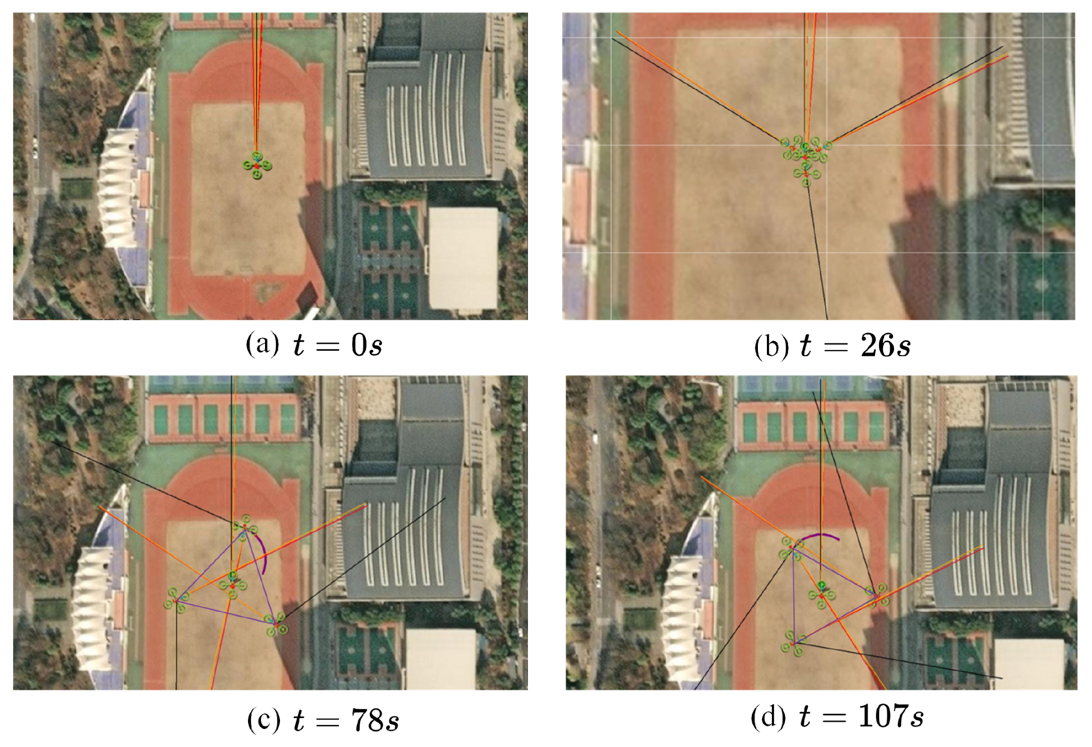
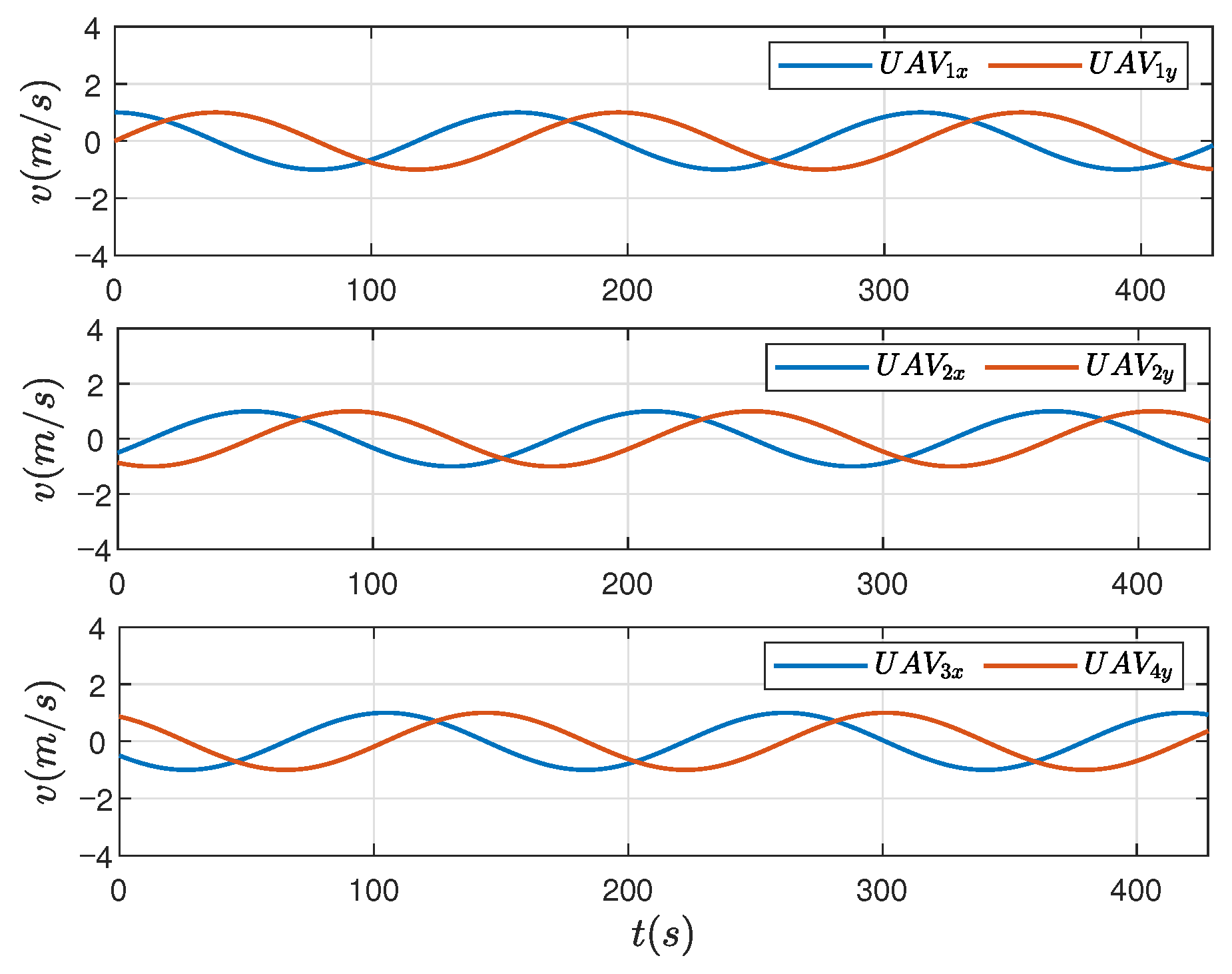
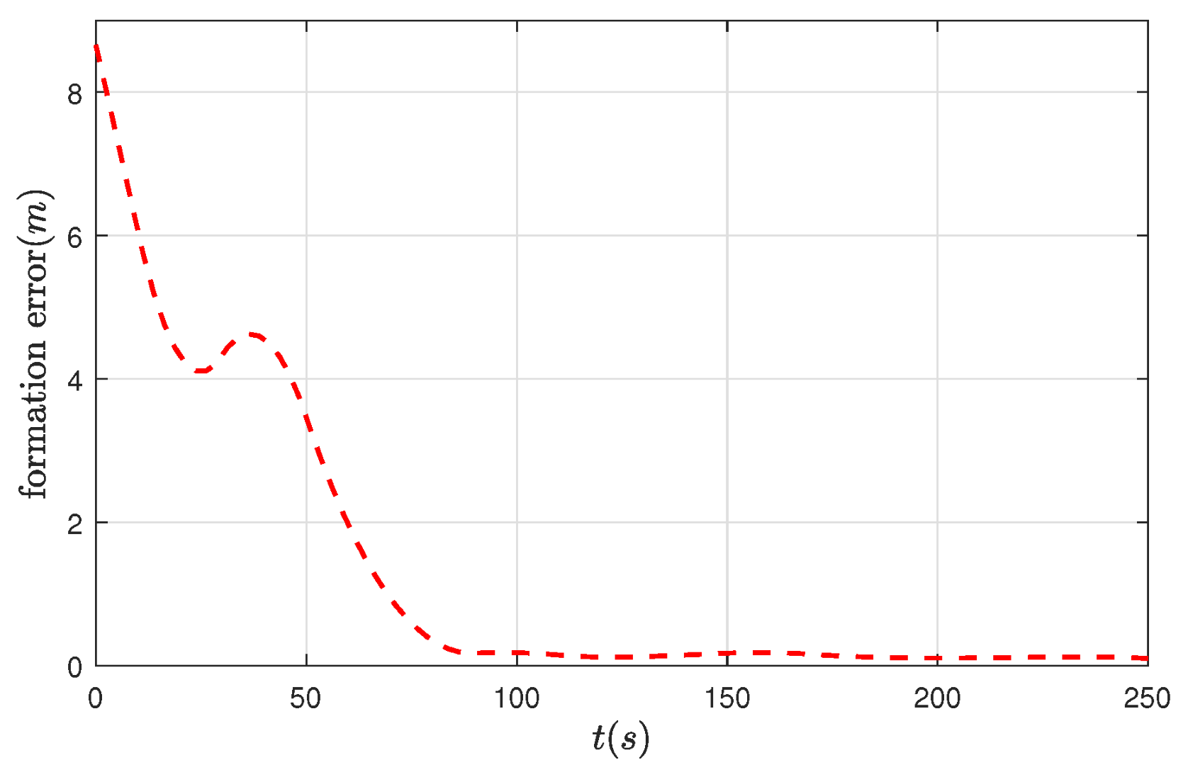
4. Example and Experimental Results

In this section, the effectiveness of the algorithm is demonstrated through numerical examples and SIL simulation experiments. Subsequently, the research limitations and future research work are presented.

4.1. Formation-Tracking Simulation Experiments and Results

In this part, several examples are presented to verify the validity of the constructed algorithm. Figure 3 presents five UAVs, where symbol 0 denotes the leader and symbols 1–4 represent the followers. Assuming that the topology graph is time-varying, the four possible topologies are denoted as ${\mathcal{G}}_{\mathsf{1}},{\mathcal{G}}_{\mathsf{2}},{\mathcal{G}}_{\mathsf{3}}$, and ${\mathcal{G}}_{\mathsf{4}}$. From Figure 3, it can be observed that each topology graph is undirected and connected. The switching sequence of the interactive topology graph is ${\mathcal{G}}_{\mathsf{1}}\to {\mathcal{G}}_{\mathsf{4}}\to {\mathcal{G}}_{\mathsf{2}}\to {\mathcal{G}}_{\mathsf{3}}\to {\mathcal{G}}_{\mathsf{1}}\to {\mathcal{G}}_{\mathsf{2}}\to {\mathcal{G}}_{\mathsf{4}}$. The switching signal is depicted in Figure 4.

The initial positions of followers are ${\mathit{x}}_1\left(t\right)={[8.112,-2.475]}^{T}m$, ${\mathit{x}}_2\left(t\right)={[6.408,7.172]}^{T}m$, ${\mathit{x}}_3\left(t\right)={[-2.240,2.467]}^{T}m$, ${\mathit{x}}_4\left(t\right)={[-3.535,5.180]}^{T}m$. The leader UAV’s initial position is $\mathit{q}\left(t\right)={[0.4278,0.4877]}^{T}m$. Meanwhile, the control input is $\left|\right|{\mathit{u}}_q\left|\right|\le 0.1$. Matrices $\mathit{A}$ and $\mathit{B}$ are chosen as $\mathit{A}=\left[\begin{array}{cccc}0& -1;& 1& 0\end{array}\right]$ and $\mathit{B}=\left[\begin{array}{cccc}0& 0;& 2& 0\end{array}\right]$, ${𝓚}_2=[0.2302,-0.7165]$, $𝓟=\left[\begin{array}{cccc}3.1125& 1;& 1& 3.1125\end{array}\right]>0$. The relevant parameters in the controller are set as $d_{ij}\left(0\right)=0.01, d_{i0}\left(0\right)=0.01$, ${\gamma }_{ij}=2.5$ and ${\gamma }_{i0}=1.4$. Meanwhile, in the triggering mechanism (6), the positive constants ${\mu }_i$ and $\omega$ are specified as ${\mu }_i=0.01, \omega =0.1$. The formation vector is ${\mathit{\delta }}_i\left(t\right)=[-10sin(t+(i-1)\pi /2);-10cos(t+(i-1)\pi /2);10cos(t+(i-1)\pi /2);-10sin(t+(i-1)\pi /2)],i=1,2,3,4.$

In the following, the results of the numerical simulation are presented. Figure 5 shows the formation-tracking trajectory of all UAVs. To visualize the trajectory changes, Figure 6 displays the position snapshots of all UAVs at $t=0 \mathrm{s}$, $t=5 \mathrm{s}$, $t=10 \mathrm{s}$, and $t=15 \mathrm{s}$. The followers are represented by “*”, “∆”, and the leader is denoted by “□”, respectively. From Figure 5 and Figure 6, it can be observed that all follower UAVs not only formed a time-varying formation but also tracked the trajectory of the leader UAV. In addition, the state errors of the UAV are depicted in Figure 7. Figure 8 shows the state information of the leader UAV and all follower UAVs. As shown in Figure 8, the non-zero leader input generates a trajectory that the follower UAV can track to the leader’s trajectory. This paper investigates the formation-tracking problem, where followers are required to track the leader’s trajectory. Therefore, based on the above analysis, we conclude that the desired TVFT configuration can be achieved. If the input of the leader is zero, it becomes a leader-less formation problem. Figure 9 illustrates the formation trajectory in the absence of leader input.

Figure 10 shows the triggering instants of the adaptive ETM and the static ETM, respectively. It is easy to observe that the proposed method has a lower triggering count. This is because the parameter $d_{ij}\left(t\right)$ in the triggering mechanism (6) is time-varying, and this adaptive coefficient is advantageous in regulating the triggering count of the system. Figure 11 represents the convergence curve of the adaptive weights. To further demonstrate the positive effect of the adaptive strategy, we conduct a comparison experiment by only removing the adaptive parameters. Specifically, the adaptive parameters are set as constants, i.e., ${\dot{d}}_{ij}\left(t\right)=0$ and ${\dot{d}}_{i0}\left(t\right)=0$. Based on this, Figure 12 shows the comparison of results with and without the adaptive technology. The results indicate that the introduction of adaptive technology can reduce the formation error more rapidly.

In

Table 1. The comparison of different control schemes.

Control Scheme	Triggering Event Count	Convergence Time $\left(\mathbf{s}\right)$
AETM	100	$2.3$
Static ETM [38]	227	$4.8$
Adaptive strategy [46]	Continuous updating	$3.4$

, we compare three different control schemes: the AETM, the static ETM, and the adaptive control strategy. The performance indexes evaluated are the triggering event count and convergence time. From Table 1, we can observe that the convergence time of the system is 2.3 s under the AETM. This shows that the AETM has obvious advantages in reducing the control overhead and accelerating the system’s stability.

Moreover, to demonstrate the benefits of the proposed scheme, we compare it with the existing work [20,47], as shown in

Table 2. The triggering event counts and convergence times of different ETMs.

	Fully Distributed AETM	Decentralized ETM in [47]	Distributed ETM in [20]
UAV1	12	82	25
UAV2	24	74	50
UAV3	12	67	72
UAV4	52	63	108
Triggering event count sum	100	286	165
Convergence time $\left(\mathrm{s}\right)$	2.3	7.9	4.6

. From Table 2, the fully distributed AETM in this paper has advantages in terms of the triggering event count and convergence time. Therefore, the distributed AETM can extend the inter-event interval and reduce the network pressure of the system.

In addition, this paper takes possible time-delay and external interference into account to verify the robustness and stability of the algorithm. Assume that the communication delay time ${\tau }_{*}=0.1 \mathrm{s}$. Meanwhile, the external disturbance is bounded and satisfies $\parallel {\sigma }_i\left(t\right)\parallel \le {\ell }_i$, where ${\ell }_i>0$, (e.g., ${\sigma }_{*}={\left[{\kappa }_{1}sin\left(\pi t\right),{\kappa }_{2}cos\left(\pi t\right)\right]}^T$ ). In

Table 3. Numerical experiments under time-delay and disturbance.

Performance Index	AETM	Time-Delay	Disturbance	Time-Delay and Disturbance
Triggering event count	100	109	106	113
Convergence time $\left(\mathrm{s}\right)$	2.30	2.49	2.38	2.58

, the experimental results show that the convergence performance of the algorithm is slightly affected by time-delay and disturbance. This suggests that the algorithm exhibits a degree of robustness. Based on a large number of experiments, we find that the system has no convergence trend when the communication delay is increased to about 0.8s. If the time delays and disturbances exceed certain thresholds, the algorithm needs to be further optimized to enhance its performance under complex conditions. In particular, real-world network delay will potentially destroy formation stability. Therefore, these factors need to be further considered in future work.

To further evaluate the algorithm’s performance, this research introduces a perturbation of $1\%$ to the experimental parameters under the switching topology. These perturbations encompass adaptive and triggering threshold parameters, intended to simulate uncertainties that may arise in real-world applications. The confidence intervals for the number of triggering events and convergence time are $(99.16,104.24)$ and $(2.1497,2.3973)$, respectively. The above analysis indicates that minor data fluctuations occur in the presence of smaller random perturbations.

On the other hand, to further validate the effectiveness of the designed algorithm at the software level, this paper conducts software simulation experiments for UAVs. The experimental platform consists of a mission planner (MP) and Ubuntu 18.04 system. Figure 13 shows the multi-UAV SIL communication framework for the MP simulation platform. Specifically, the detailed experimental parameters include a flight altitude of $4\mathrm{m}$ and a vehicle airspeed of $1 \mathrm{m}/\mathrm{s}$. Other hardware devices and parameters are listed in

Table 4. Main experimental parameters of UAV via MP simulation platform.

Parameter	Value
MP-GCS version	$1.3.74$
UAV model	Quadrotor $F450$
Flight control software	Ardupilot Mega 3.6.11
Data transmission protocol	$NMEA0183$
Baud rate of serial port	115,200 HZ
Number of quadrotors	4
Flight altitude	4 m
Vehicle_airspeed	1 m/s
Initial location	(0 m, 0 m, 0 m)

. The simulation test lasts approximately 2.5 min (including UAV initialization, takeoff, formation, and tracking). The simulation experiment is performed on a computer with an AMD 5800H CPU and an Nvidia GTX 3050 GPU. Figure 14 presents the formation trajectory snapshots of four quadrotor UAVs in the MP at different times. Similar to Figure 6, it can be observed from Figure 14 that all follower UAVs (i.e., $UA{V}_1$, $UA{V}_2$, $UA{V}_3$) track the trajectory of the leader $UA{V}_4$ at time $t=107 \mathrm{s}$, meanwhile completing the circular formation motion. Figure 15 presents the velocity variations in all follower UAVs. Figure 16 displays the formation error of UAV in the SIL simulation. As a result, it is demonstrated that the expected TVFT configuration is achieved from the software perspective. In summary, the validity of the designed algorithm is verified by numerical examples and SIL simulation experiments.

4.2. Future Work

This paper builds an SIL simulation platform, which effectively compensates for the shortage of physical hardware. However, it should be emphasized that although real firmware of UAVs is utilized in the simulation, the interference and random factors in real-world environments have not been adequately considered. In addition, the checking of event-triggered conditions needs to calculate the state errors in real time, which might increase the computational complexity of the algorithm. Therefore, in future work, multi-threading and distributed computing techniques will be employed to further alleviate the computational complexity. On the other hand, this paper assumes that the communication topology is always connected. However, communication links in the real world may be intermittently interrupted when subjected to cyber-attacks. Therefore, fault-tolerant control is a promising solution. In practical applications, the main potential challenges and corresponding solutions requiring consideration include:

(1) Adaptability of algorithms to real hardware: The computing power and sensor accuracy of actual UAV may differ from those in the simulation environment. Meanwhile, the real-world model of UAV is affected by physical limitations such as actuator failure and control saturation. This divergence has the potential to impact the performance of the algorithm. During the design phase, the algorithm should consider the compatibility with hardware and the performance limitation brought by hardware.

(2) Handling of communication delays and packet loss: In real-world scenarios, communication delays and data packet loss are prevalent issues. The algorithms must be capable of adapting to these network characteristics to uphold the stability and reliability of the system.

(3) Adaptability to environmental disturbances and dynamic changes: Real-world environmental disturbances (e.g., signal interference, etc.) might affect the flight control of the UAV. Thus, the algorithm needs to be robust enough to deal with these uncertainties. In addition, external environmental interference also includes GPS positioning accuracy, airflow disturbance, wind speed, etc. Therefore, by using ultra-wide-band (UWB) signals instead of GPS signals and carrying high-precision sensors such as TFmini plus (TF) fixed-height radar to reduce the UAV hardware and external environment interference might be a good solution.

(4) Safety and reliability: In practical applications, the communication link may be interrupted by disturbances such as cyber-attacks. Thus, it is necessary to integrate fault detection and fault-tolerant mechanisms [26] into algorithms to ensure that UAVs can operate safely even when faced with partial system failures.

5. Conclusions

In this paper, the TVFT problem of MUSs with non-zero leader input has been investigated, and sufficient conditions for realizing the formation-tracking configuration have been obtained. Firstly, an AETM was designed for the formation-tracking problem. Compared with a single adaptive technique or an ETM, the combination of these two strategies effectively reduced the consumption of network resources. Meanwhile, the convergence time of formation tracking has been shortened. Secondly, unlike previous studies without considering leader inputs, this paper considered the non-zero leader inputs, which increased the flexibility of formation-tracking trajectories. Meanwhile, the formation-tracking feasibility conditions have been extended. In addition, the designed consensus protocol is also suitable for the switching topology. This extension enhanced the robustness and adaptability of the consensus protocol. Finally, the validity of the constructed algorithm was further verified by numerical examples and SIL simulation experiments. In future work, exploring the secure consensus of formation tracking under cyber-attacks is an interesting task. Furthermore, another aspect of future work is to consider the implementation of control strategies in outdoor flight experiments with UAVs.

References

1. Guo, J.; Zhang, J.; Wang, Z.; Liu, X.; Zhou, S.; Shi, G.; Shi, Z. Formation cooperative intelligent tactical decision making based on bayesian network model. Drones 2024, 8, 427. [Google Scholar] [CrossRef]
2. Zou, Y.; An, Q.; Miao, S.; Chen, S.; Wang, X.; Su, H. Flocking of uncertain nonlinear multi-agent systems via distributed adaptive event-triggered control. Neurocomputing 2021, 465, 503–513. [Google Scholar]
3. Liang, H.; Zhang, L.; Sun, Y.; Huang, T. Containment control of semi-Markovian multiagent systems with switching topologies. IEEE Trans. Syst. Man Cybern. Syst. 2021, 51, 3889–3899. [Google Scholar]
4. Roman-Figueroa, C.; Bravo, L.; Paneque, M.; Navia, R.; Cea, M. Chemical products for crop protection against freezing stress: A review. J. Agron. Crop Sci. 2021, 207, 391–403. [Google Scholar]
5. Ouyang, Q.; Wu, Z.; Cong, Y.; Wang, Z. Formation control of unmanned aerial vehicle swarms: A comprehensive review. Asian J. Control 2022, 25, 570–593. [Google Scholar]
6. Tang, X.; Yu, J.; Li, X.; Dong, X.; Ren, Z. Distributed formation control with obstacle avoidance for multiple underactuated unmanned surface vehicles. J. Frankl. Inst. 2024, 12, 107008. [Google Scholar]
7. Yang, S.; Yu, W.; Liu, Z.; Ma, F. A robust hybrid iterative learning formation strategy for multi-unmanned aerial vehicle systems with multi-operating modes. Drones 2024, 8, 406. [Google Scholar] [CrossRef]
8. Xia, L.; Li, Q.; Song, R.; Zhang, Z. Leader-follower time-varying output formation control of heterogeneous systems under cyber attack with active leader. Inf. Sci. 2022, 585, 24–40. [Google Scholar]
9. Yang, Y.; Xiong, X.; Yan, Y. UAV formation trajectory planning algorithms: A review. Drones 2024, 7, 62. [Google Scholar]
10. Wen, J.; Yang, J.; Li, Y.; He, J.; Li, Z.; Song, H. Behavior-based formation control digital twin for multi-AUG in edge computing. IEEE Trans. Netw. Sci. Eng. 2023, 10, 2791–2801. [Google Scholar]
11. Amirkhani, A.; Barshooi, A.H. Consensus in multi-agent systems: A review. Artif. Intell. Rev. 2021, 55, 3897–3935. [Google Scholar]
12. Zhang, P.; Xue, H.; Gao, S.; Zhang, J. Distributed adaptive consensus tracking control for multi-agent system with communication constraints. IEEE Trans. Parallel Distrib. Syst. 2021, 32, 1293–1306. [Google Scholar]
13. Cao, Y.; Yu, W.; Ren, W.; Chen, G. An overview of recent progress in the study of distributed multi-agent coordination. IEEE Trans. Ind. Inform. 2013, 9, 427–438. [Google Scholar]
14. Chang, Z.; Xue, H.; Liang, H.; Zhang, P. Time-varying formation control for nonlinear multi-agent systems against actuator attacks. J. Frankl. Inst. 2022, 359, 11068–11088. [Google Scholar]
15. Liang, H.; Cheng, W. Adaptive Formation Regulation for Multi-agent Systems with Structure Uncertainties via Variable Recombination. In Proceedings of the 2020 Chinese Automation Congress (CAC), Shanghai, China, 6–8 November 2020; IEEE: Piscataway, NJ, USA, 2021; pp. 5873–5878. [Google Scholar]
16. Yan, C.; Zhang, W.; Guo, H.; Zhu, F.; Qian, Y. Distributed adaptive time-varying formation control for Lipschitz nonlinear multi-agent systems. Trans. Inst. Meas. Control 2021, 44, 272–285. [Google Scholar]
17. Lippay, Z.S.; Hoagg, J.B. Formation control with time-varying formations, bounded controls, and local collision avoidance. IEEE Trans. Control Syst. Technol. 2021, 30, 261–276. [Google Scholar]
18. Dong, X.; Yu, B.; Shi, Z.; Zhong, Y. Time-varying formation control for unmanned aerial vehicles: Theories and applications. IEEE Trans. Control Syst. Technol. 2015, 23, 340–348. [Google Scholar]
19. Wang, J.; Han, L.; Li, X.; Dong, X.; Li, Q.; Ren, Z. Time-varying formation of second-order discrete-time multi-agent systems under non-uniform communication delays and switching topology with application to UAV formation flying. IET Control Theory Appl. 2020, 14, 1947–1956. [Google Scholar]
20. Wang, J.H.; Xu, Y.L.; Zhang, J.; Yang, D.D. Time-varying formation for general linear multi-agent systems via distributed event-triggered control under switching topologies. Chin. Phys. B 2018, 27, 040504. [Google Scholar]
21. Sun, L.; Liu, X.; Tan, W.; Deng, Y.; Jiao, J.; Zhao, M. Predictive state observer-based aircraft distributed formation tracking considering input delay and saturations. Drones 2024, 8, 23. [Google Scholar] [CrossRef]
22. Cao, H.; Han, L.; Li, D.; Hu, Q. Fully distributed dynamic event-triggering formation control for multi-agent systems under DoS attacks: Theory and experiment. Neurocomputing 2023, 552, 126546. [Google Scholar]
23. Li, Q.; Hua, Y.; Dong, X.; Ren, Z. Time-varying formation tracking control for unmanned aerial vehicles: Theories and applications. IFAC PapersOnLine 2022, 55, 49–54. [Google Scholar]
24. Wang, Y.; Lei, Y.; Bian, T.; Guan, Z. Distributed control of nonlinear multiagent systems with unknown and nonidentical control directions via event-triggered communication. IEEE Trans. Cybern. 2020, 50, 1820–1832. [Google Scholar] [PubMed]
25. Liu, C.; Liu, L.; Cao, J.; Abdel-Aty, M. Intermittent event-triggered optimal leader-following consensus for nonlinear multi-agent systems via actor-critic algorithm. IEEE Trans. Neural Netw. Learn. Syst. 2021, 34, 3992–4006. [Google Scholar]
26. Guo, X.; Wang, B.; Wang, J.; Wu, Z.; Guo, L. Adaptive event-triggered PIO-based anti-disturbance fault-tolerant control for MASs With process and sensor faults. IEEE Trans. Netw. Sci. Eng. 2024, 11, 77–88. [Google Scholar]
27. Hu, W.; Yang, C.; Huang, T.; Gui, W. A distributed dynamic event-triggered control approach to consensus of linear multiagent systems with directed networks. IEEE Trans. Cybern. 2020, 50, 869–874. [Google Scholar]
28. Ding, C.; Zhang, Z.; Zhang, J. Dynamics event-triggered-based time-varying bearing formation Control for UAVs. Drones 2024, 8, 185. [Google Scholar] [CrossRef]
29. Li, W.; Zhang, H.; Wang, W.; Cao, Z. Fully distributed event-triggered time-varying formation control of multi-agent systems subject to mode-switching denial-of-service attacks. Appl. Math. Comput. 2022, 414, 126645. [Google Scholar]
30. Li, M.; Zhang, W.; Yan, C.; Hu, Z. Observer-based bipartite formation control for MASs with external disturbances under event-triggered scheme. IEEE Trans. Circuits Syst. II Express Br. 2022, 69, 1178–1182. [Google Scholar]
31. Li, X.; Chen, M.Z.Q.; Su, H.; Li, C. Distributed bounds on the algebraic connectivity of graphs with application to agent networks. IEEE Trans. Cybern. 2017, 47, 2121–2131. [Google Scholar]
32. Xia, L.; Li, Q.; Song, R. Adaptive event-triggered average tracking control with activable event-triggering mechanisms. IEEE Trans. Syst. Man Cybern. Syst. 2023, 53, 6067–6079. [Google Scholar]
33. Xu, M.; Li, M.; Hao, F. Fully distributed optimization of second-order systems with disturbances based on event-triggered control. Asian J. Control 2023, 25, 3715–3728. [Google Scholar]
34. Li, X.; Dong, X.; Li, Q.; Ren, Z. Event-triggered time-varying formation control for general linear multi-agent systems. J. Frankl. Inst. 2019, 356, 10179–10195. [Google Scholar]
35. Deng, J.; Li, K.; Wu, S.; Wen, Y. Distributed adaptive time-varying formation tracking control for general linear multi-agent systems based on event-triggered strategy. IEEE Access 2020, 8, 13204–13217. [Google Scholar]
36. Dou, L.; Cai, S.; Zhang, X.; Su, X.; Zuang, R. Event-triggered-based adaptive dynamic programming for distributed formation control of multi-UAV. J. Frankl. Inst. 2022, 359, 3671–3691. [Google Scholar]
37. Wu, Z.; Xu, Y.; Lu, R.; Wu, Y.; Huang, T. Event-triggered control for consensus of multiagent systems with fixed/switching topologies. IEEE Trans. Syst. Man Cybern. Syst. 2018, 48, 1736–1746. [Google Scholar]
38. Huang, J.; Chen, L.; Xie, X.; Wang, M.; Xu, B. Distributed event-triggered consensus control for heterogeneous multi-agent systems under fixed and switching topologies. Int. J. Control Autom. Syst. 2019, 17, 1945–1956. [Google Scholar]
39. Zhang, J.; Zhang, H.; Gao, Z.; Sun, S. Time-varying formation control with general linear multi-agent systems by distributed event-triggered mechanisms under fixed and switching topologies. Neural Comput. Appl. 2022, 34, 4277–4294. [Google Scholar]
40. Li, Y.; Liu, X.; Liu, H.; Du, C.; Lu, P. Distributed dynamic event-triggered consensus control for multi-agent systems under fixed and switching topologies. J. Frankl. Inst. 2021, 358, 4348–4372. [Google Scholar]
41. Hua, Y.; Dong, X.; Li, Q.; Ren, Z. Distributed adaptive formation tracking for heterogeneous multiagent systems with multiple nonidentical leaders and without well-informed follower. Int. J. Robust Nonlinear Control 2020, 30, 2131–2151. [Google Scholar]
42. Song, W.; Feng, J.; Zhang, H.; Xu, X. Event-based formation control of heterogeneous multiagent systems with leader agent of nonzero input. Inf. Sci. 2022, 598, 157–181. [Google Scholar]
43. Hua, Y.; Dong, X.; Hu, G.; Li, Q.; Ren, Z. Distributed time-varying output formation tracking for heterogeneous linear multiagent systems with a nonautonomous leader of unknown input. IEEE Trans. Autom. Control 2019, 64, 4292–4299. [Google Scholar]
44. Zhang, J.; Zhang, H.; Sun, S.; Cai, Y. Adaptive time-varying formation tracking control for multiagent systems with nonzero leader input by intermittent communications. IEEE Trans. Cybern. 2022, 53, 5706–5715. [Google Scholar]
45. Zhang, X.; Wu, J.; Zhan, X.; Han, T.; Yan, H. Event-triggered adaptive time-varying formation tracking of multi-agent system with a leader of nonzero input. IEEE Trans. Circuits Syst. II Express Br. 2023, 70, 6. [Google Scholar]
46. Wang, R.; Dong, X.; Li, Q.; Zhang, R. Distributed adaptive control for time-varying formation of general linear multi-agent systems. Int. J. Syst. Sci. 2017, 48, 3491–3503. [Google Scholar]
47. Yang, D.; Ren, W.; Liu, X.; Chen, W. Decentralized event-triggered consensus for linear multi-agent systems under general directed graphs. Automatica 2016, 69, 242–249. [Google Scholar]
Figure 1. Time-varying formation-tracking task in the X-Y plane.
Drones 09 00259 g001
Figure 2. The overall framework of the AETM.
Drones 09 00259 g002
Figure 3. The topology variation in the system.
Drones 09 00259 g003
Figure 4. The topology switching signal σ ( t ) of system.
Drones 09 00259 g004
Figure 5. Formation tracking trajectory under the AETM.
Drones 09 00259 g005
Figure 6. The trajectory snapshots of all UAVs in the x y plane at different times.
Drones 09 00259 g006
Figure 7. First-state and second-state errors for UAVs.
Drones 09 00259 g007
Figure 8. State information for the leader UAV and follower UAVs.
Drones 09 00259 g008
Figure 9. Formation trajectories without leader input.
Drones 09 00259 g009
Figure 10. The triggering instants for each UAV under different strategies. (a) Adaptive ETM, (b) Static ETM.
Drones 09 00259 g010
Figure 11. The trajectory snapshots of all UAVs in the x-y plane at different times.
Drones 09 00259 g011
Figure 12. First-state and second-state errors for UAVs.
Drones 09 00259 g012
Figure 13. The communication framework of multi-UAV based on MP simulation platform. (Note: Four UAVs are simulated on the MP software. Different UDP ports distinguish different UAVs and the MAVProxy protocol is used to connect the UAVs to the MP software 1.3.74. Meanwhile, the DroneKit tool is utilized to compose control commands for initiating the UAV).
Drones 09 00259 g013
Figure 14. SIL simulation of UAV formation trajectory snapshots at time t = 0   s , t = 26   s , t = 78   s , t = 107   s . (Note: A total of four UAVs (i.e., U A V 1 , U A V 2 , U A V 3 , U A V 4 ) perform formation-tracking tasks on the MP platform. UAV4 is the leader and the rest are the followers. The followers need to track the leader’s trajectory while completing the circular formation. The whole experiment process includes three stages: (a) UAV initialization and unlocking ( t = 0   s ), (b) take-off ( t = 26   s ), (c) formation-building ( t = 78   s ), (d) formation tracking ( t = 107   s )).
Drones 09 00259 g014
Figure 15. Velocity variations in all follower UAVs under SIL simulation.
Drones 09 00259 g015
Figure 16. The formation error in SIL simulation.
Drones 09 00259 g016