BiLSTM-Attention-PFTBD: Robust Long-Baseline Acoustic Localization for Autonomous Underwater Vehicles in Adversarial Environments

Abstract

The accurate and reliable localization and tracking of Autonomous Underwater Vehicles (AUVs) are essential for the success of various underwater missions, such as environmental monitoring, subsea resource exploration, and military operations. long-baseline acoustic localization (LBL) is a fundamental technique for underwater positioning, but it faces significant challenges in adversarial environments. These challenges include abrupt target maneuvers and intentional signal interference, both of which degrade the performance of traditional localization algorithms. Although particle filter-based Track-Before-Detect (PFTBD) algorithms are effective under normal submarine conditions, they struggle to maintain accuracy in adversarial environments due to their dependence on conventional likelihood calculations. To address this, we propose the BiLSTM-Attention-PFTBD algorithm, which enhances the traditional PFTBD framework by integrating bidirectional Long Short-Term Memory (BiLSTM) networks with multi-head attention mechanisms. This combination enables better feature extraction and adaptation for localizing AUVs in adversarial underwater environments. Simulation results demonstrate that the proposed method outperforms traditional PFTBD algorithms, significantly reducing localization errors and maintaining robust tracking accuracy in adversarial settings.

1. Introduction

Autonomous Underwater Vehicles (AUVs) are critical for a wide range of underwater applications [1,2], including environmental monitoring, subsea resource exploration, and military operations. Accurate localization and tracking are fundamental to ensuring mission success. Long-baseline acoustic localization (LBL) is a widely adopted technique for underwater positioning, which estimates the AUV’s position by measuring the time-of-arrival (TOA) of acoustic signals at multiple buoys and applying spherical intersection methods [3,4]. Despite its effectiveness in stable environments, LBL suffers from performance degradation in challenging conditions such as low signal-to-noise ratio (SNR), multipath propagation, and environmental noise [5,6].

In response, several signal processing techniques have been developed to improve localization accuracy. Direct Sound Selection (DSS) methods enhance TOA estimation by isolating direct paths in multipath environments, improving the robustness of acoustic measurements [7,8,9]. Advanced matched filtering techniques, such as Multidimensional Matched Filtering (MMF) [10], Phase Matched Filtering (PMF) [11], and Adaptive Matched Filtering (AMF) [12], offer improvements under harsh acoustic conditions. However, these methods are still limited by low SNR and multipath effects, especially in dynamic environments. Combining course, speed, and distance measurements has been used to improve positioning accuracy, particularly by optimizing positioning results through geodetic adjustment methods [11]. In an effort to reduce the accuracy of low-cost navigation equipment commonly used in underwater vehicle navigation, Naus et al. [13] proposed a method that combined course, speed, and distance measurements to improve positioning accuracy.

Track-Before-Detect (TBD) methods, which process raw sensor data to directly estimate target trajectories, offer a promising alternative to traditional threshold-based detection, which can be unreliable in noisy environments [14,15]. Particle filter-based TBD (PFTBD) [16] has proven effective for underwater target tracking, especially in environments with weak signals. However, most existing TBD methods, including PFTBD, assume cooperative targets and favorable environmental conditions. This reliance on ideal conditions makes them prone to performance degradation in adversarial scenarios, where targets employ evasive maneuvers and signal interference [17], which are commonly encountered in real-world applications [18].

Recent advancements in machine learning have significantly enhanced the localization capabilities of Autonomous Underwater Vehicles (AUVs). Liu et al. [19] introduced a reinforcement learning-based approach that optimizes beacon selection and energy distribution to improve both accuracy and efficiency. Stefaniedou et al. [20] comparatively analyzed the application of a linear model (LM) composed of linear layers and a convolutional model (CM) consisting of convolutional layers and linear layers in the deep reinforcement learning (DRL) method, and proposed a comprehensive framework for path planning in complex 3D underwater environments. Yao et al. [21] combined Convolutional Neural Networks, bidirectional Long Short-Term Memory, and a Time-Varying Attention layer, using a Nonlinear Kepler Optimization Algorithm to optimize hyperparameters for improved prediction accuracy. Additionally, Li et al. [22] integrated Long Short-Term Memory with an Extended Kalman Filter for system identification and employed a Nonlinear Explicit Complementary Filter for attitude estimation, achieving sensor-independent navigation.

As we all know, deep learning methods usually demand a large quantity of labeled data, consume significant computational resources, and involve a high degree of black box nature. These issues limit their practical application in resource-constrained scenarios. To address this, we chose to correct traditional algorithms with deep learning-based methods. This approach achieves a balance, combining the advantages of both traditional and deep learning methods, ensuring high localization accuracy while maintaining relatively low computational complexity.

In this paper, we propose a novel hybrid approach, the BiLSTM-Attention-PFTBD algorithm, which integrates bidirectional Long Short-Term Memory (BiLSTM) networks and multi-head attention mechanisms with the PFTBD framework. By combining the strengths of traditional tracking methods with the adaptability of deep learning, we address the following key issues: the insufficient accuracy of traditional algorithms in adversarial environments and the high computational cost of deep learning. Specifically, we apply deep learning corrections on top of the traditional algorithm’s fast response, reducing the complexity of training and ensuring high localization accuracy. This hybrid approach ensures both system efficiency and robustness, improving localization performance, particularly in adversarial and dynamic underwater environments.

Our method introduces several key innovations:

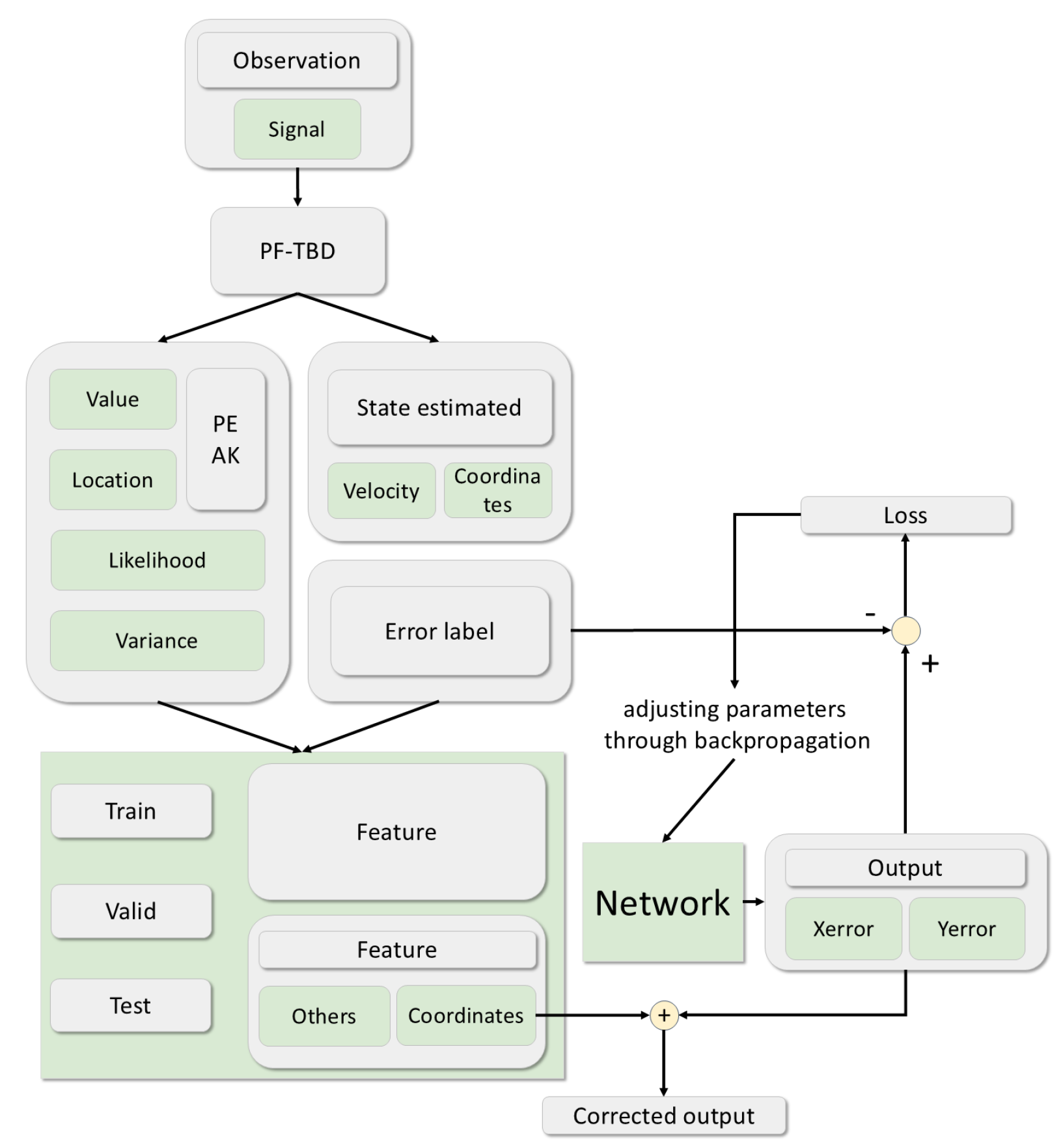
• Enhanced localization accuracy through the integration of direct signals and comprehensive feature extraction: The proposed method utilizes both raw measurements and derived features from particle filtering. The system integrates normalized likelihood computation and peak detection analysis to enhance system robustness in adverse conditions. For detailed explanations, see Section 5.1.
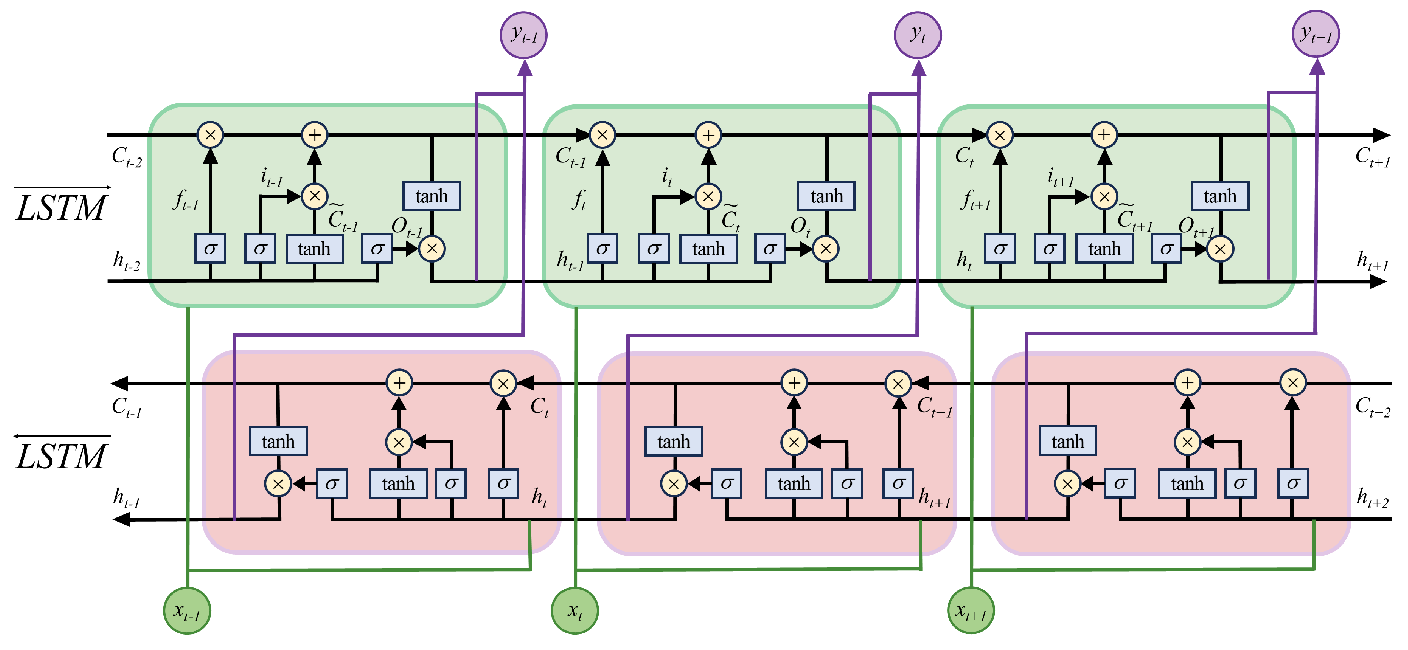
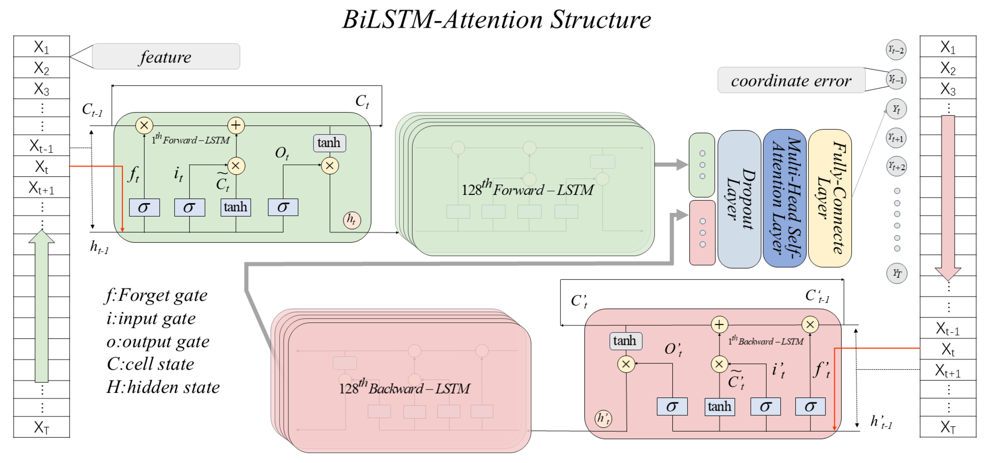
• Advanced temporal modeling with BiLSTM for the detection of abrupt maneuvers and signal losses: Conventional tracking systems often fail with complex temporal dynamics and dispersed information. Our BiLSTM architecture processes sequences bidirectionally, enabling the effective prediction of abrupt maneuvers and signal losses in adversarial environments.
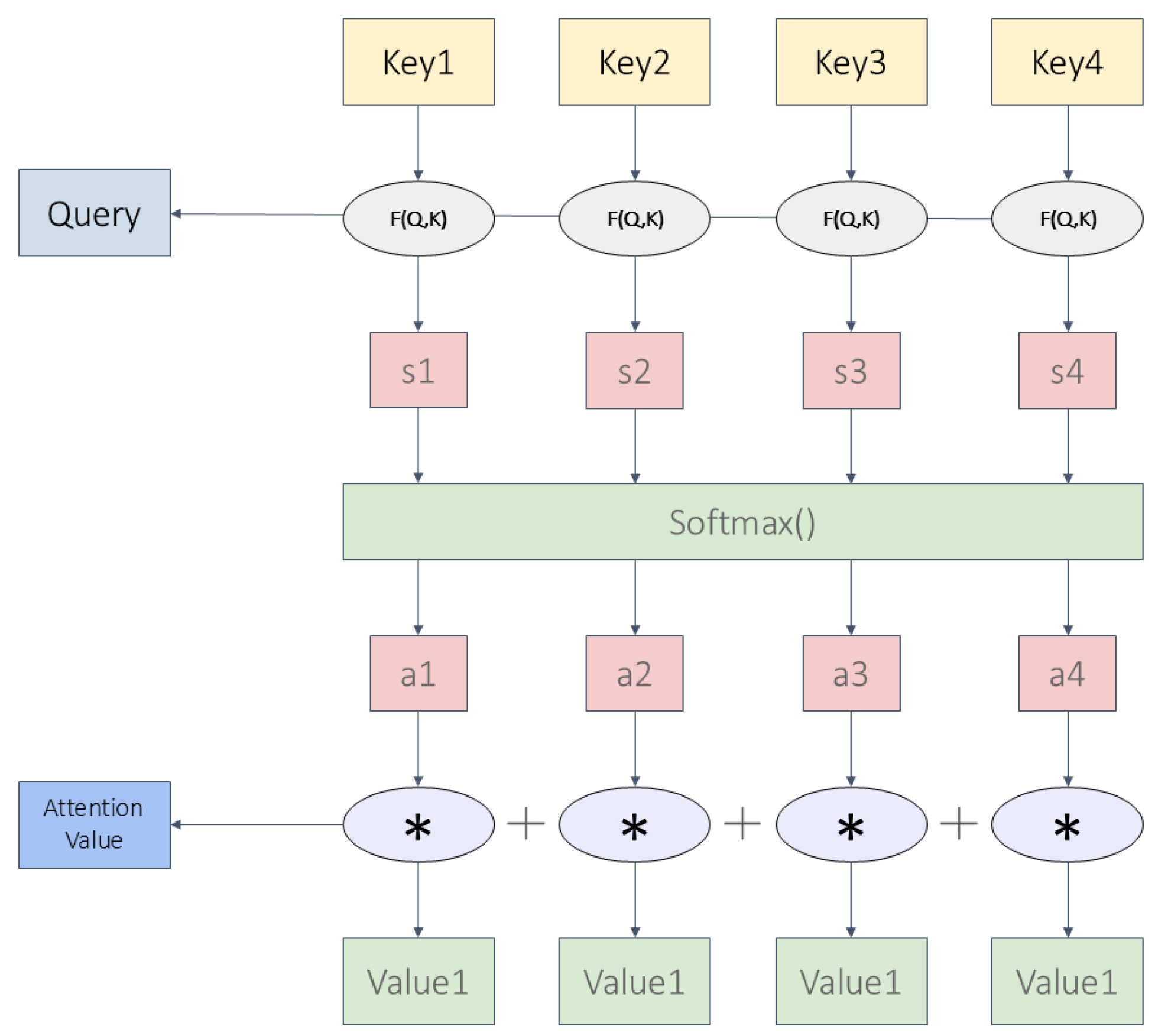
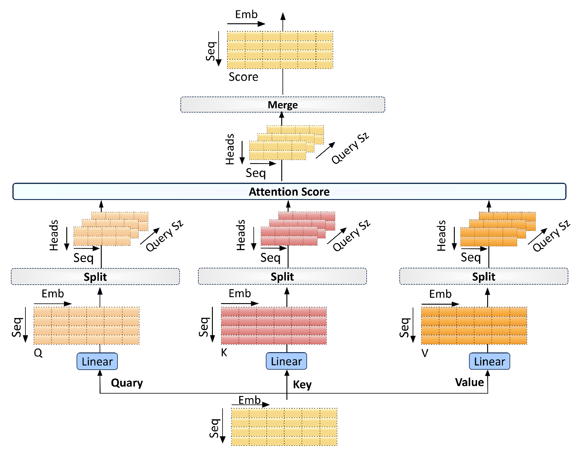
• Capturing complex dependencies with multi-head attention mechanisms: Traditional models struggle with dispersed temporal dependencies and complex data interactions. Our multi-head attention mechanism examines multiple sequence positions simultaneously, enabling dynamic focus adjustment and effective pattern recognition in challenging environments.

The remainder of this paper is organized as follows: Section 2 reviews conventional particle filtering methods for underwater localization. Section 3 analyzes the limitations of these methods in adversarial scenarios. Section 4 presents the deep learning components, including BiLSTM and multi-head attention, used to enhance tracking performance. Section 5 introduces our approach, the BiLSTM-Attention-PFTBD algorithm. Section 6 discusses simulation results and performance analysis. Finally, Section 7 concludes the paper and outlines future research directions.

2. Particle Filtering Localization

To understand the limitations of traditional algorithms in adversarial environments, we revisit the particle filtering (PF) approach for target localization.

2.1. Particle Filtering for State Estimation

PF is a sequential Monte Carlo method widely used to estimate the posterior distribution of a system’s state in nonlinear and non-Gaussian environments. In TOA tracking-based detection systems, PF estimates the target’s state by propagating a set of particles, each representing a hypothesis of the target’s position and velocity [23].

At time step k, the system generates N particles ${\{X_k^i,w_k^i\}}_{i=1}^N$, where each particle $X_k^i$ carries a weight $w_k^i$. The particle $X_k^i$ at time k is defined as

$$X_k^i=\left[\begin{array}{c}{x}_k^i\\ y_k^i\\ v_{x,k}^i\\ v_{y,k}^i\end{array}\right],$$

(1)

where $x_k^i$ and $y_k^i$ represent the x and y coordinates of the target’s position, while $v_{x,k}^i$ and $v_{y,k}^i$ represent the velocities in the x and y directions. Each particle $X_k^i$ is assigned a weight $w_k^i$ that quantifies the likelihood of the particle representing the true target state based on current observations.

2.2. Particle Initialization

To initiate the particles, we first establish an initial position estimate by applying a discretized grid across the localization area. The area, with dimensions L by W, is divided into grids of size d. For each grid point, the likelihood function $p(x,y)$ is computed-based on signals received from four buoys, using the formula provided in Section 2.4. The grid point $(x,y)$ with the highest likelihood is selected as the initial position estimate.

Following this, particle positions are set using a polar coordinate framework. Both the range r and the bearing angle $\theta$ are sampled uniformly: r is drawn from a uniform distribution between 0 and the maximum range $r_{\max }$, while $\theta$ is uniformly sampled between $0^{\circ }$ and ${360}^{\circ }$. Particle velocities are also initialized in polar coordinates, with speed v uniformly distributed from 0 to the maximum speed $v_{\max }$, and the velocity angle $\varphi$ sampled over $0^{\circ }$ to ${360}^{\circ }$.

The Cartesian coordinates $(x_k^i,y_k^i)$ of each particle’s position and the velocity components $(v_{x,k}^i,v_{y,k}^i)$ are determined via the transformations as

$$\begin{array}{cc}\hfill x_k^i& =r_i·cos\left({\theta }_i\right)+x_0,\hfill \end{array}$$

(2)

$$\begin{array}{cc}\hfill y_k^i& =r_i·sin\left({\theta }_i\right)+y_0,\hfill \end{array}$$

(3)

$$\begin{array}{cc}\hfill v_{x,k}^i& =v_i·cos\left({\varphi }_i\right),\hfill \end{array}$$

(4)

$$\begin{array}{cc}\hfill v_{y,k}^i& =v_i·sin\left({\varphi }_i\right),\hfill \end{array}$$

(5)

where $(x_0,y_0)$ is the estimated initial position, and i denotes the particle index.

2.3. Prediction Step for State

In the prediction phase, particles evolve over time using a motion model, typically assuming constant velocity. The state of each particle at time step k is predicted using

$$X_k^i=\mathbf{F}{X}_{k-1}^i+\Gamma {\mathbf{w}}_k^i,$$

(6)

where $X_k^i$ represents the state vector of the i-th particle at time step k, including both position and velocity components. The term $\mathbf{F}$ is the state transition matrix, and $\Gamma$ represents the impact of random accelerations modeled as process noise.

The state transition matrix $\mathbf{F}$ and control matrix $\Gamma$ are defined as

$$\mathbf{F}=\left[\begin{array}{cccc}1& T& 0& 0\\ 0& 1& 0& 0\\ 0& 0& 1& T\\ 0& 0& 0& 1\end{array}\right],\Gamma =\left[\begin{array}{cc}{\displaystyle \frac{T^2}{2}}& 0\\ T& 0\\ 0& {\displaystyle \frac{T^2}{2}}\\ 0& T\end{array}\right],$$

(7)

where T is the time interval between successive measurements. Here, $\mathbf{F}$ updates the position and velocity states, assuming constant velocity, and $\Gamma$ accounts for the influence of acceleration on the state.

The noise term ${\mathbf{w}}_k^i$ is a white noise vector, simulating random acceleration to account for uncertainties in particle motion. Specifically, ${\mathbf{w}}_k^i={\left[\begin{array}{c}{a}_k^{x,i},a_k^{y,i}\end{array}\right]}^T$, where $a_k^{x,i}$ and $a_k^{y,i}$ are random acceleration components along the x and y axes, respectively. These components add variability to the prediction, capturing unmodeled dynamics or environmental effects.

Incorporating the noise term ${\mathbf{w}}_k^i$ effectively mitigates uncontrollable factors introduced by natural environmental variations, such as the complexities of underwater environments. This additional variability helps capture minor deviations and uncertainties, enhancing tracking robustness under typical conditions. However, in adversarial environments where abrupt target maneuvers and sharp velocity changes occur, these adjustments are often insufficient. The constant velocity assumption still fails to account for rapid, intentional movements, leading to potential inaccuracies in state prediction and divergence in particle trajectories.

2.4. Update Step for Particle Weight

After prediction, particle weights are updated based on how well the predicted states match the new observations. The weight update follows Bayes’ theorem, i.e.,

$$w_k^i=w_{k-1}^i·{\displaystyle \frac{p\left(z_k\right|X_k^i)}{p\left(z_k\right|z_{1:k-1})}}.$$

(8)

In Equation (8), $w_k^i$ represents the updated weight of the i-th particle at time k, calculated by adjusting the previous weight $w_{k-1}^i$ of that particle based on the likelihood $p\left(z_k\right|X_k^i)$ of observing $z_k$ given the particle’s predicted state $X_k^i$. This likelihood term reflects how well the particle’s predicted state matches the observation. The denominator $p\left(z_k\right|z_{1:k-1})$ serves as a normalization factor to ensure that the sum of all particle weights equals 1, thereby maintaining a valid probability distribution across the particles.

The likelihood $p\left(z_k\right|X_k^i)$ represents the probability of receiving the observation $z_k$ given the predicted state of particle $X_k^i$. For localization based on multiple buoys, the overall likelihood can be expressed as the product of the matched filtering outputs from all buoys, yielding

$$p\left(z_k\right|X_k^i)=\prod _{m=1}^M{e}_{k,m}^i,$$

(9)

where $e_{k,m}^i$ is the matched filtering output for the i-th particle at the m-th buoy, and M is the total number of buoys.

The TOA for the i-th particle at buoy m is calculated as

$${\tau }_{m,k}^i={\displaystyle \frac{\sqrt{{(x_k^i-x_{m,k})}^2+{(y_k^i-y_{m,k})}^2}}{\widehat{c}}},$$

(10)

where $x_{m,k}$ and $y_{m,k}$ are the coordinates of buoy m at time k, and $\widehat{c}$ is the estimated speed of sound in the medium.

To convert the continuous TOA value into a discrete index for matched filtering, the following equation is used

$$a_{m,k}^i=⌊{\tau }_{m,k}^i·f_s⌋+1,$$

(11)

where $\lfloor ·\rfloor$ represents the floor function, and $f_s$ is the sampling frequency.

This discrete index $a_{m,k}^i$ is then used to locate the corresponding amplitude $e_{k,m}^i$ by applying the matched filter to the received signal.

In adversarial environments, however, signal jamming can distort or obscure the amplitude $e_{k,m}^i$, resulting in inaccurate weight updates and thus reducing the effectiveness of the filter. Inaccurate TOA estimates due to target maneuvers or jamming effects can further lead to misalignment in matched filtering, compromising the likelihood computation and affecting overall tracking accuracy.

2.5. Resampling Implementation

To address particle degeneracy, resampling is applied when only a few particles carry significant weight. The effective particle number ($N_{\mathrm{eff}}$) is calculated as

$$N_{\mathrm{eff}}={\displaystyle \frac{1}{{\sum }_{i=1}^N{\left(w_k^i\right)}^2}}.$$

(12)

If $N_{\mathrm{eff}}$ falls below a threshold (typically $0.8N$), systematic resampling is performed to avoid particle impoverishment.

2.6. State Estimation

Finally, the target’s state is estimated by calculating the weighted average of the particles’ positions and velocities as

$${\widehat{X}}_k=\sum _{i=1}^N{w}_k^i{X}_k^i,$$

(13)

where ${\widehat{X}}_k$ is the estimated state of the target at time k. However, in adversarial environments, the accumulated errors from inaccurate predictions and weight updates due to target maneuvers and signals can lead to significant estimation errors.

In the next section, we will provide a detailed description of the adversarial environment and analyze the performance of current algorithms in such settings.

3. Limitations of Traditional Particle Filters in Adversarial Environments

Traditional particle filters (PFs) rely on accurate motion models and reliable observations. In adversarial environments, these assumptions are often violated due to abrupt target maneuvers and signal jamming. Such disruptions cause prediction errors, particle divergence, and reduced filter performance.

3.1. Mathematical Formulation of the Problem

The state-space model of a target tracking system is typically defined by the state transition and observation equations

$$\begin{array}{cc}\hfill {\mathbf{x}}_k& =f\left({\mathbf{x}}_{k-1}\right)+{\mathbf{w}}_k,\hfill \end{array}$$

(14)

$$\begin{array}{cc}\hfill {\mathbf{z}}_k& =h\left({\mathbf{x}}_k\right)+{\mathbf{v}}_k,\hfill \end{array}$$

(15)

where ${\mathbf{x}}_k$ is the state vector at time k, ${\mathbf{z}}_k$ is the observation vector, $f(·)$ and $h(·)$ are the state transition and observation functions, respectively. ${\mathbf{w}}_k$ and ${\mathbf{v}}_k$ represent process and measurement noises, typically modeled as Gaussian with covariances $\mathbf{Q}$ and $\mathbf{R}$ [24,25].

In adversarial environments, two main challenges disrupt the traditional PF framework: abrupt target maneuvers and signal loss.

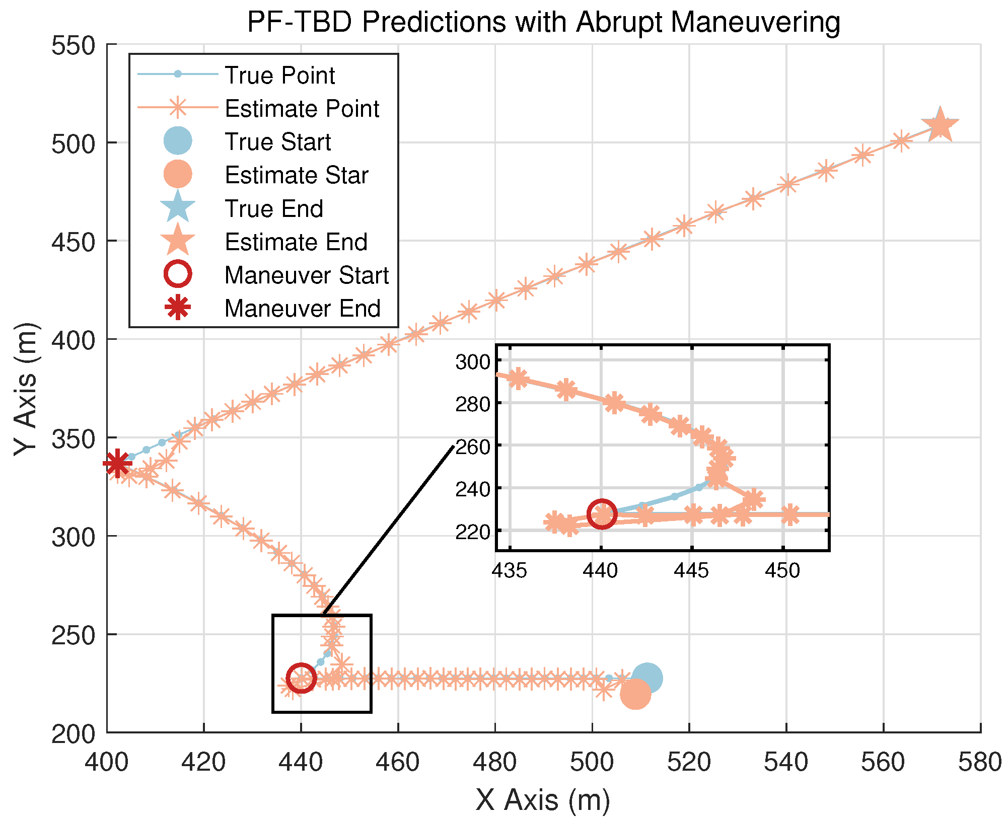
3.2. Impact of Abrupt Maneuvers

Abrupt maneuvers refer to abrupt changes in the target’s velocity or direction, which are not captured by the assumed motion model $f(·)$. Mathematically, under abrupt maneuvers, the true state evolution can be expressed as

$${\mathbf{x}}_k=f\left({\mathbf{x}}_{k-1}\right)+{\Delta }_k+{\mathbf{w}}_k,$$

(16)

where ${\Delta }_k$ represents the maneuvering acceleration, an unknown and unpredictable input [26]. Traditional PFs, which rely on the fixed motion model $f(·)$, cannot account for ${\Delta }_k$, resulting in a state prediction error

$${\mathbf{e}}_k^{\mathrm{pred}}={\Delta }_k.$$

(17)

The error in (17) can lead to a divergence between the predicted state distribution $p\left({\mathbf{x}}_k\right|{\mathbf{z}}_{1:k-1})$ and the true state distribution $p\left({\mathbf{x}}_k\right)$. The Kullback–Leibler (KL) divergence quantifies this discrepancy

$$D_{\mathrm{KL}}(p_{\mathrm{true}}\parallel p_{\mathrm{pred}})=\int p_{\mathrm{true}}\left({\mathbf{x}}_k\right)log\left({\displaystyle \frac{p_{\mathrm{true}}\left({\mathbf{x}}_k\right)}{p_{\mathrm{pred}}\left({\mathbf{x}}_k\right)}}\right)d{\mathbf{x}}_k\gg 0.$$

(18)

A large $D_{\mathrm{KL}}$ indicates poor tracking performance. Figure 1 shows the tracking errors during maneuver transitions, highlighting the limitations of traditional PFs.

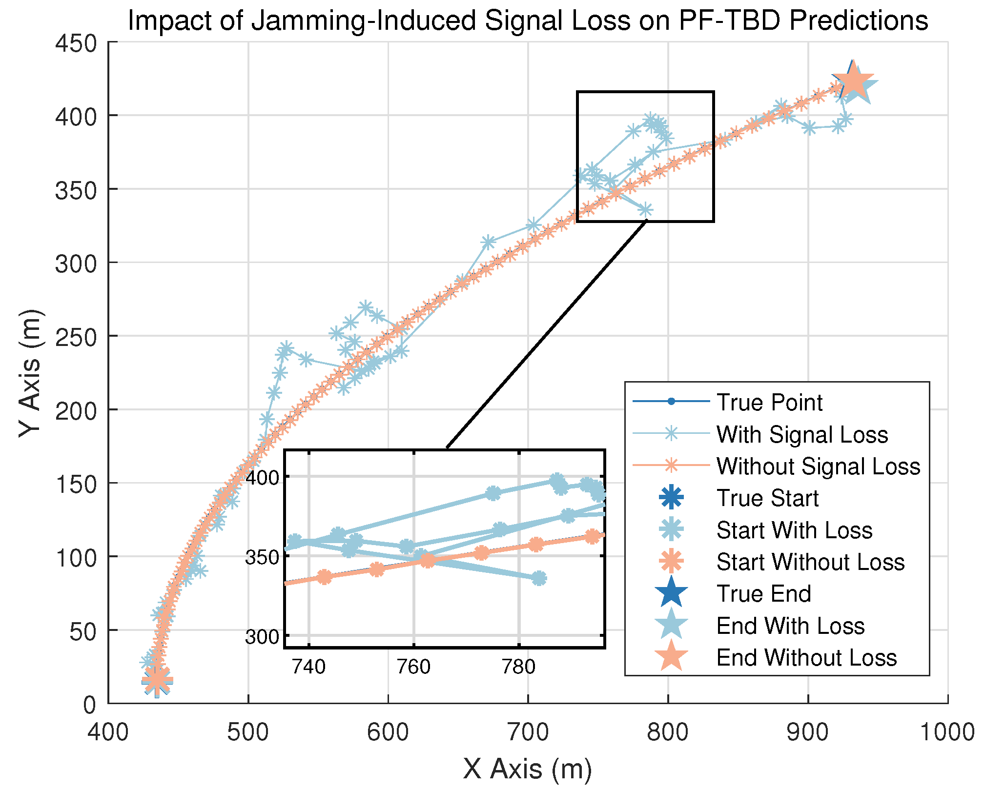
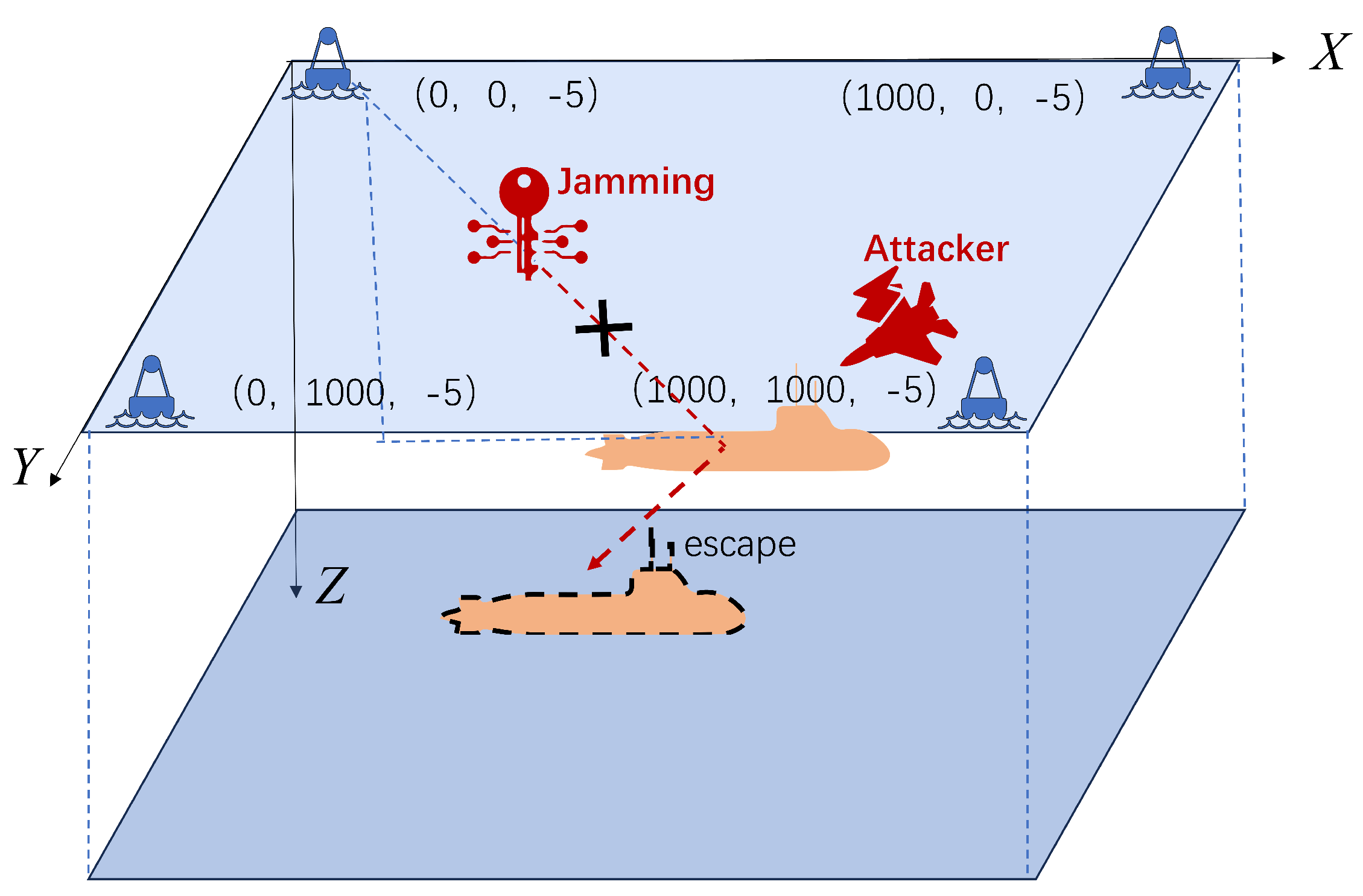
3.3. Effect of Signal Jamming

Signal jamming introduces corruptions to the observations, modifying the observation model as:

$${\mathbf{z}}_k=h\left({\mathbf{x}}_k\right)+{\mathbf{v}}_k+{\mathit{\eta }}_k,$$

(19)

where ${\mathit{\eta }}_k$ represents the jamming. The measurement error becomes:

$${\mathbf{e}}_k^{\mathrm{obs}}={\mathbf{v}}_k+{\mathit{\eta }}_k.$$

(20)

This results in inaccurate likelihood calculations, affecting the weight update step:

$$w_k^i=w_{k-1}^i·p\left({\mathbf{z}}_k\right|{\mathbf{x}}_k^i).$$

(21)

The skewed likelihood due to ${\mathit{\eta }}_k$ causes particle impoverishment. Figure 2 demonstrates the impact of signal jamming on tracking performance.

Full-band jamming overwhelms signal peaks in Figure 3, rendering PFTBD algorithms dependent on peak detection, as shown in Equation (9), inoperable through catastrophic signal-to-noise ratio degradation, thereby inducing severe target tracking errors.

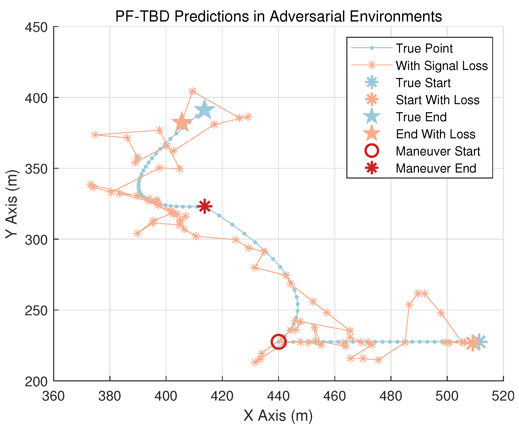
3.4. Severity of Adversarial Conditions

The combined effect of abrupt maneuvers and intentional jamming introduces several critical issues. The unknown ${\Delta }_k$ creates substantial uncertainty in state prediction, which the traditional PF cannot accommodate. Furthermore, the jamming ${\mathit{\eta }}_k$ results in measurement noise deviating from Gaussian assumptions, rendering likelihood calculations unreliable. These factors collectively lead to the degeneracy of particles, where misleading weights due to incorrect likelihoods cause particle depletion.

As illustrated in Figure 4, the performance of traditional particle filter (PF) algorithms degrades significantly in scenarios involving abrupt maneuvers and intermittent signal loss. These challenges underscore the limitations of conventional PF approaches in maintaining reliable tracking under complex adversarial conditions. Therefore, relying solely on traditional particle filtering is insufficient for effective target tracking under adversarial conditions. It necessitates integrating advanced methods that can adapt to dynamic changes and handle corrupted or missing data.

4. Deep Learning to Enhance Particle Filter Performance

By leveraging deep learning, tracking becomes a time-series prediction task [27,28], enabling better management of uncertainties in target motion.This section introduces the deep learning mechanisms involved in enhancing PFTBD performance, including LSTM, BiLSTM, attention mechanism, and multi-head attention mechanism.

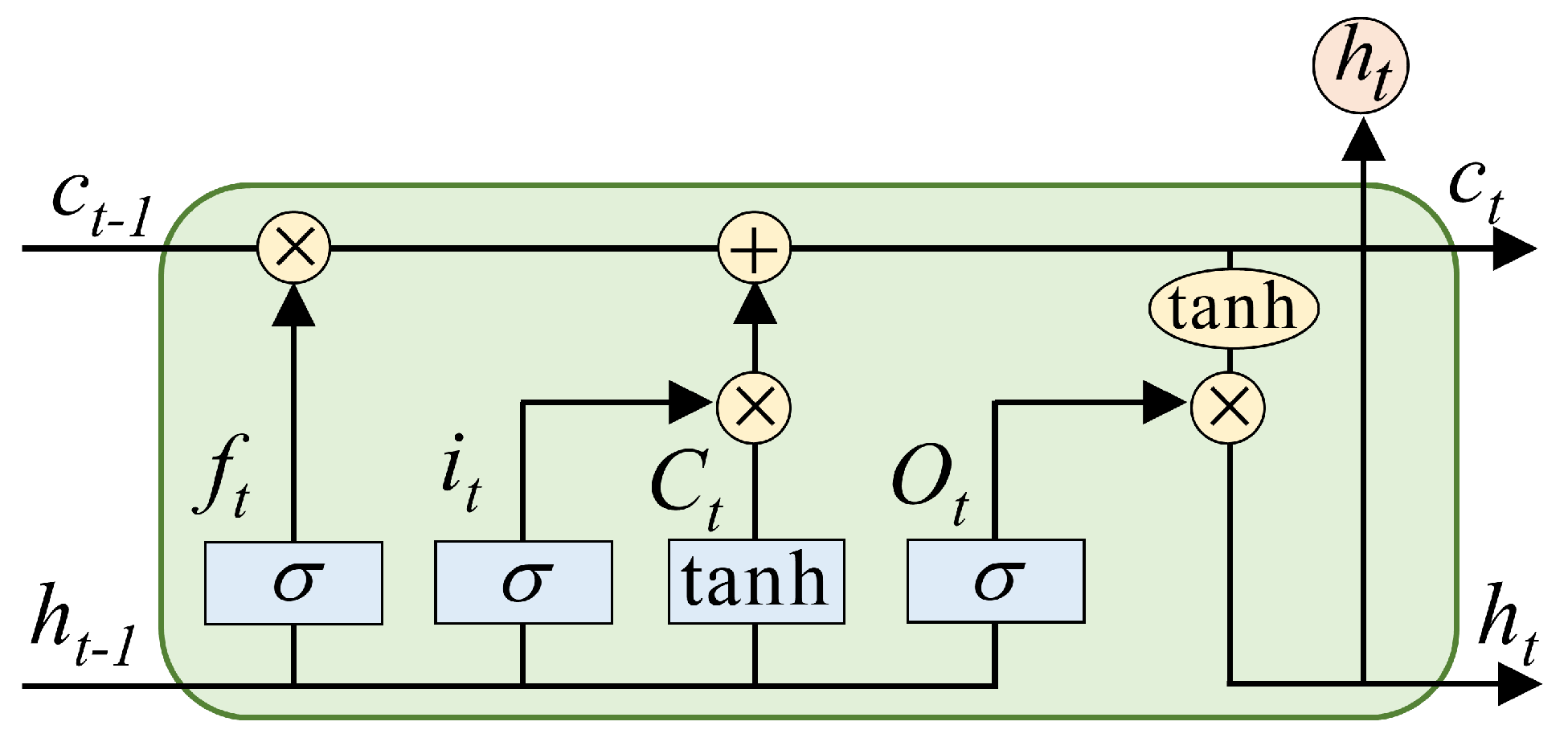
4.1. LSTM Cell Structure

Long Short-Term Memory (LSTM) is a widely used variant of Recurrent Neural Networks (RNNs), designed to overcome the vanishing gradient and exploding gradient problems commonly encountered in traditional RNNs. As shown in Figure 5, LSTM introduces memory cells and three key gating mechanisms—forget gate, input gate, and output gate—which manage the flow of information. This structure allows LSTMs to selectively retain or discard information across time steps, making them well suited for sequential data tasks.

The operations within a single LSTM cell at time step t are defined by the following equations

$$\begin{array}{cc}\hfill f_t& =\sigma (W_f[h_{t-1},x_t]+b_f),(\mathrm{Forget}\mathrm{Gate})\hfill \end{array}$$

(22)

$$\begin{array}{cc}\hfill i_t& =\sigma (W_i[h_{t-1},x_t]+b_i),(\mathrm{Input}\mathrm{Gate})\hfill \end{array}$$

(23)

$$\begin{array}{cc}\hfill {\tilde{C}}_t& =tanh(W_c[h_{t-1},x_t]+b_c),(\mathrm{Cell}\mathrm{Candidate})\hfill \end{array}$$

(24)

$$\begin{array}{cc}\hfill C_t& =f_t\odot C_{t-1}+i_t\odot {\tilde{C}}_t,(\mathrm{Cell}\mathrm{State}\mathrm{Update})\hfill \end{array}$$

(25)

$$\begin{array}{cc}\hfill o_t& =\sigma (W_o[h_{t-1},x_t]+b_o),(\mathrm{Output}\mathrm{Gate})\hfill \end{array}$$

(26)

$$\begin{array}{cc}\hfill h_t& =o_t\odot tanh\left(C_t\right).(\mathrm{Hidden}\mathrm{State})\hfill \end{array}$$

(27)

The key terms in these equations include $f_t$, $i_t$, and $o_t$, which represent the activations of the forget gate, input gate, and output gate, respectively. The input at time step t is denoted by $x_t$, and $h_{t-1}$ is the hidden state from the previous time step. The candidate cell state, used to update the cell state, is ${\tilde{C}}_t$. The updated cell state, which combines the previous state $C_{t-1}$ with the new input, is $C_t$. Finally, the current hidden state $h_t$ is influenced by the output gate and the updated cell state.

4.2. BiLSTM Network Structure

BiLSTM (bidirectional LSTM) networks, as shown in Figure 6, extend the LSTM architecture by processing the input sequence in both forward and reverse directions. The hidden states from the forward ${\overrightarrow{h}}_t$ and backward ${\overleftarrow{h}}_t$ LSTM layers are concatenated to form the final hidden state $h_t$

$$\begin{array}{cc}\hfill \overrightarrow{h_t}& ={\mathrm{LSTM}}_{\mathrm{forward}}(x_1,x_2,\dots ,x_t),\hfill \end{array}$$

(28)

$$\begin{array}{cc}\hfill \overleftarrow{h_t}& ={\mathrm{LSTM}}_{\mathrm{backward}}(x_T,x_{T-1},\dots ,x_t),\hfill \end{array}$$

(29)

$$\begin{array}{cc}\hfill h_t& =[\overrightarrow{h_t},\overleftarrow{h_t}].\hfill \end{array}$$

(30)

This bidirectional processing allows BiLSTM networks to leverage both past and future context in time-series data, which is particularly useful in underwater localization tasks where signal jamming or target maneuvers can depend on both prior and future data points.

4.3. Attention Mechanism

The attention mechanism, shown in Figure 7, enables the model to dynamically focus on specific parts of an input sequence, particularly useful for tasks where input relevance varies. The attention mechanism operates by computing the similarity between queries (Q) and keys (K), followed by applying a softmax function to generate attention weights. The formulation is as follows:

$$\mathrm{Attention}(Q,K,V)=\mathrm{softmax}\left({\displaystyle \frac{Q{K}^T}{\sqrt{d_k}}}\right)V,$$

(31)

where Q, K, and V represent linear projections of the input sequence, and $d_k$ denotes the dimensionality of K. The scaling factor $\sqrt{d_k}$ maintains stability during training by adjusting the range of values in the dot product similarity calculation. The softmax normalizes these similarities into probabilities, thereby determining attention weights, which are then used to compute a weighted sum with V, generating the output of the attention layer.

4.4. Multi-Head Attention Mechanism

The multi-head attention mechanism, as illustrated in Figure 8, extends the single attention function by using multiple independent attention heads to process distinct aspects of the input sequence in parallel, allowing the model to capture complex dependencies and relationships within the data. Each head i computes attention independently as

$${\mathrm{head}}_i=\mathrm{Attention}({\mathbf{Q}}_i,{\mathbf{K}}_i,{\mathbf{V}}_i),$$

(32)

where ${\mathbf{Q}}_i=\mathbf{X}{\mathbf{W}}_Q^i$, ${\mathbf{K}}_i=\mathbf{X}{\mathbf{W}}_K^i$, and ${\mathbf{V}}_i=\mathbf{X}{\mathbf{W}}_V^i$ are the Query, Key, and Value matrices for head i, with ${\mathbf{W}}_Q^i$, ${\mathbf{W}}_K^i$, and ${\mathbf{W}}_V^i$ as the respective projection matrices.

The outputs of all heads are concatenated and passed through a final linear transformation to obtain the multi-head attention output, yielding

$$\mathrm{MultiHead}(Q,K,V)=\mathrm{Concat}({\mathrm{head}}_1,\dots ,{\mathrm{head}}_h){\mathbf{W}}_O,$$

(33)

where ${\mathbf{W}}_O$ is the output projection matrix that consolidates the information from each head.

This multi-head structure enables the model to capture richer and more complex data dependencies by attending to multiple subspaces of the input sequence simultaneously. In adversarial contexts, such as environments with signal jamming or abrupt target maneuvers, the multi-head attention mechanism allows the model to dynamically adjust its focus, enabling it to handle the complexities of target tracking in challenging and unpredictable adversarial environments.

In the following sections, we will discuss how these components are integrated into our proposed algorithm and the improvements they bring to PFTBD performance.

5. Our Approach

The overall architecture of our proposed BiLSTM-Attention-PFTBD algorithmis shown in Figure 9. This framework combines a BiLSTM-Attention network with PFTBD, leveraging deep learning to enhance localization accuracy and robustness. In this section, we will provide a detailed explanation of the key steps of the proposed algorithm.

5.1. Signal Features for Network Input

After the particle filter updates the particle weights, several important features are extracted from the process of PFTBD, as described in Section 2, to serve as inputs to the network. These features help the network predict future errors and refine localization estimates.

5.1.1. Estimated Position and Velocity

The estimated state of the target at time step k is computed as the weighted average of the particles’ positions and velocities, as shown in Equation (13)

$$\begin{array}{cc}\hfill {\widehat{x}}_k& =\sum _{i=1}^N{w}_k^i{x}_k^i,{\widehat{y}}_k=\sum _{i=1}^N{w}_k^i{y}_k^i,\hfill \end{array}$$

(34)

$$\begin{array}{cc}\hfill {\widehat{v}}_{x_k}& =\sum _{i=1}^N{w}_k^i{v}_{x_k}^i,{\widehat{v}}_{y_k}=\sum _{i=1}^N{w}_k^i{v}_{y_k}^i.\hfill \end{array}$$

(35)

5.1.2. Position and Velocity Variance

After calculating the final weighted state, we compute the relevant numerical feature: variance. To quantify the uncertainty in the particle estimates, the variance of the particle positions and velocities is calculated as follows:

$${\sigma }_x^2=\sum _{i=1}^N{w}_k^i{(x_k^i-{\widehat{x}}_k)}^2,{\sigma }_y^2=\sum _{i=1}^N{w}_k^i{(y_k^i-{\widehat{y}}_k)}^2,$$

(36)

$${\sigma }_{v_x}^2=\sum _{i=1}^N{w}_k^i{(v_{x_k}^i-{\widehat{v}}_{x_k})}^2,{\sigma }_{v_y}^2=\sum _{i=1}^N{w}_k^i{(v_{y_k}^i-{\widehat{v}}_{y_k})}^2.$$

(37)

Note that higher variance indicates greater uncertainty in the estimated state, which is crucial information for the network to improve prediction accuracy.

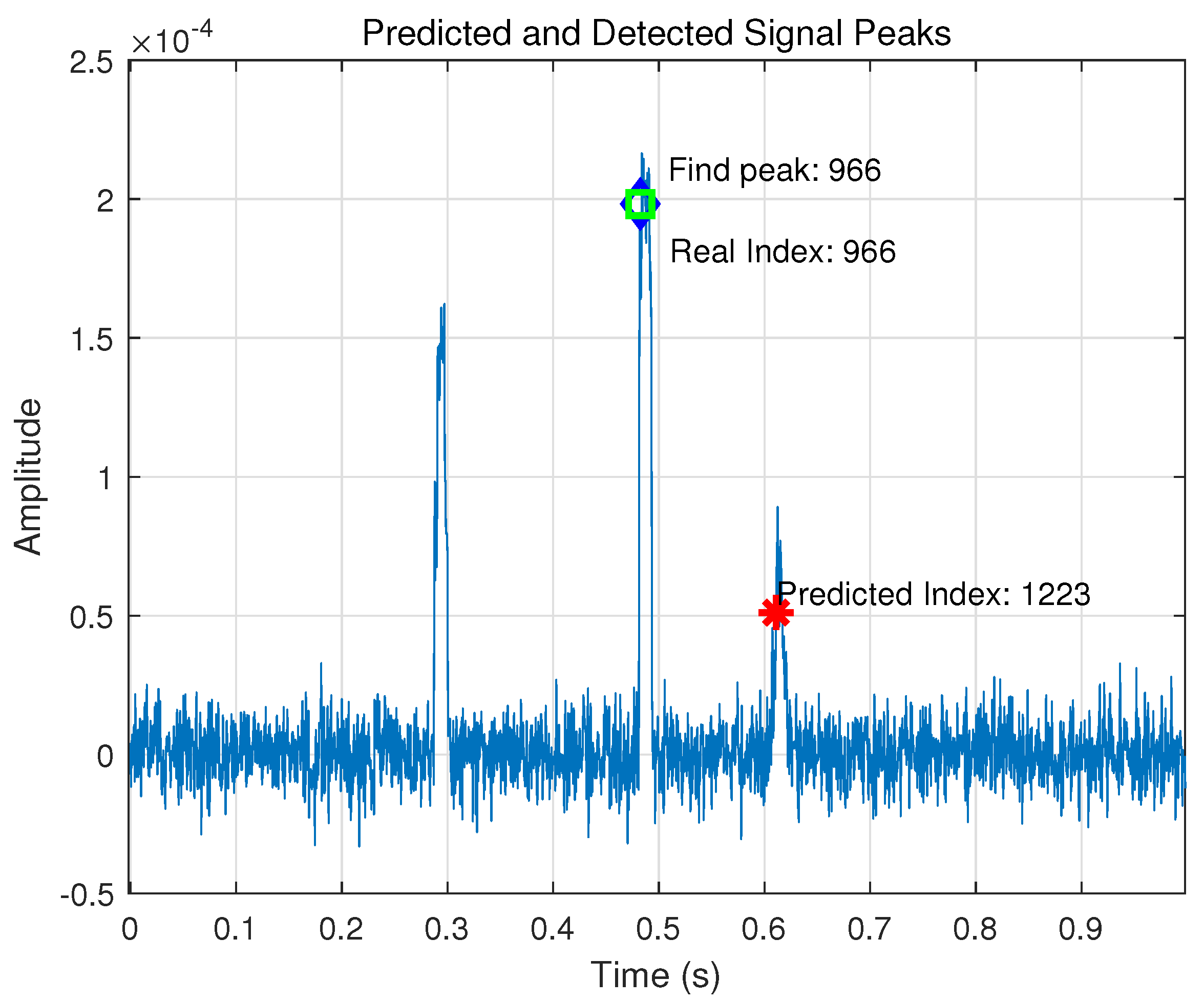
5.1.3. Signal Peak Information

In addition to position and velocity estimates, the peak times and amplitudes of the received acoustic signals at the hydrophones provide valuable information about the TOA and implicitly convey spatial information. Specifically, signal characteristics follow the principle of propagation loss, where greater distances result in increased attenuation, leading to smaller peak values and longer arrival times at more distant hydrophones. This effect allows us to infer relative distances based on the peak characteristics, where a signal received with a smaller amplitude and later time suggests a greater distance from each source. The signal peak features include

$$\mathrm{Peak}{\mathrm{Time}}_m,\mathrm{Peak}{\mathrm{Value}}_m,\mathrm{for}m=1,2,\dots ,M,$$

(38)

where M represents the number of hydrophones, which can vary depending on the configuration.

5.1.4. Likelihood Value Feature Extraction for Each Hydrophone

The likelihood function, as discussed in Section 2.4, evaluates how well the predicted TOA of the particles aligns with the observed signal peaks detected at each hydrophone. This alignment score is crucial in the particle filter update step, as it directly impacts the weight adjustment of each particle.

Once the likelihood value is calculated, the feature can be normalized as

$$L_{m,i}={\displaystyle \frac{e_{k,m}^i}{\mathrm{Peak}{\mathrm{Value}}_m}}.$$

(39)

Figure 10 shows an example where the extracted feature (Find Peak) aligns closely with the actual TOA (Real Index), while the predicted index is generated by PF-TBD, as shown in Equation (11). This visual example highlights the effectiveness of using the detected peak feature for corrective adjustments in TOA estimation.

Moreover, by normalizing the predicted index relative to the peak value, we mitigate jamming caused by signal loss, as shown in Figure 3. This approach ensures that the matching score remains comparable across the hydrophones, even when one or more hydrophones experience signal degradation. This normalization creates a standardized metric that allows for a meaningful comparison of matching accuracy, regardless of individual signal conditions.

5.2. BiLSTM-Attention for Error Prediction

The BiLSTM-Attention model uses the extracted features to predict future localization errors and correct the particle filter estimates. By learning from past target states and signal data, the BiLSTM-Attention network adapts to abrupt maneuvers and signal loss, providing robust tracking in adversarial underwater environments.

As shown in Figure 11, the model consists of forward and backward LSTM layers, which process sequential input data in both directions. The forward LSTM processes data from time step 1 to T, while the backward LSTM processes data from time step T to 1.

The hidden states from both directions are concatenated and passed through a multi-head attention mechanism, which assigns importance weights to each time step and the multiple features within it. This mechanism allows the model to selectively focus on the most relevant parts of the input sequence, both temporally and across different feature dimensions.

By prioritizing critical time steps and key feature components, this approach enhances tracking accuracy and reliability, even in challenging and unpredictable environments.

After the attention layer, the output is passed through fully connected layers to predict future localization errors. This output is then used to update the particle filter’s estimates, enabling the model to adapt to abrupt target motions or signal loss.

5.3. Error Correction with Network

Let ${\widehat{X}}_k$ be the particle filter’s state estimate and $\Delta X_k$ be the error predicted by the network. The corrected state can be formulated as

$${\widehat{X}}_k^{\mathrm{corrected}}={\widehat{X}}_k+\Delta X_k,$$

(40)

where $\Delta X_k$ represents the correction applied to the particle filter’s state estimate based on the network’s prediction, ensuring more accurate localization under dynamic and noisy conditions.

6. Simulation and Results

6.1. Simulation and Experimental Setup

To evaluate the algorithm, we simulated a controlled environment with key spatial and acoustic parameters for underwater tracking, as outlined in

Table 1. Simulation environment parameters.

Parameter	Value
Simulation Area	1000 m × 1000 m
Localization System	Long Baseline (LBL)
Buoy Positions	[(0, 0, −5), (1000, 0, −5),
	(1000, 1000, −5), (0, 1000, −5)]
Water Depth	200 m
Sound Speed	1520 m/s
Carrier Frequency	37.5 kHz
Number of Particles	2500
Max Range ($R_{\max }$)	20 m
Max Velocity ($v_{\max }$)	20 m/s
Signal-to-Noise Ratio (SNR)	−12 dB
Pulse Repetition Frequency (PRF)	1 Hz
Pulse Repetition Time (PRT)	1 s
Pulse Width	10 ms
Pulse Bandwidth	100 Hz
Sampling Rate ($f_s$)	2 kHz
Waveform	Rectangular Pulse
Bottom Loss	10 dB
Number of Paths	10

and illustrated in Figure 12. This setup provides a structured basis for assessing the algorithm’s performance in realistic underwater conditions.

6.2. Dataset Construction

The construction of the dataset is crucial for deep learning. To effectively simulate adversarial environments, we incorporated abrupt evasive maneuvers that mimic typical responses during pursuits, along with periodic random signal loss to represent signal jamming phenomena.

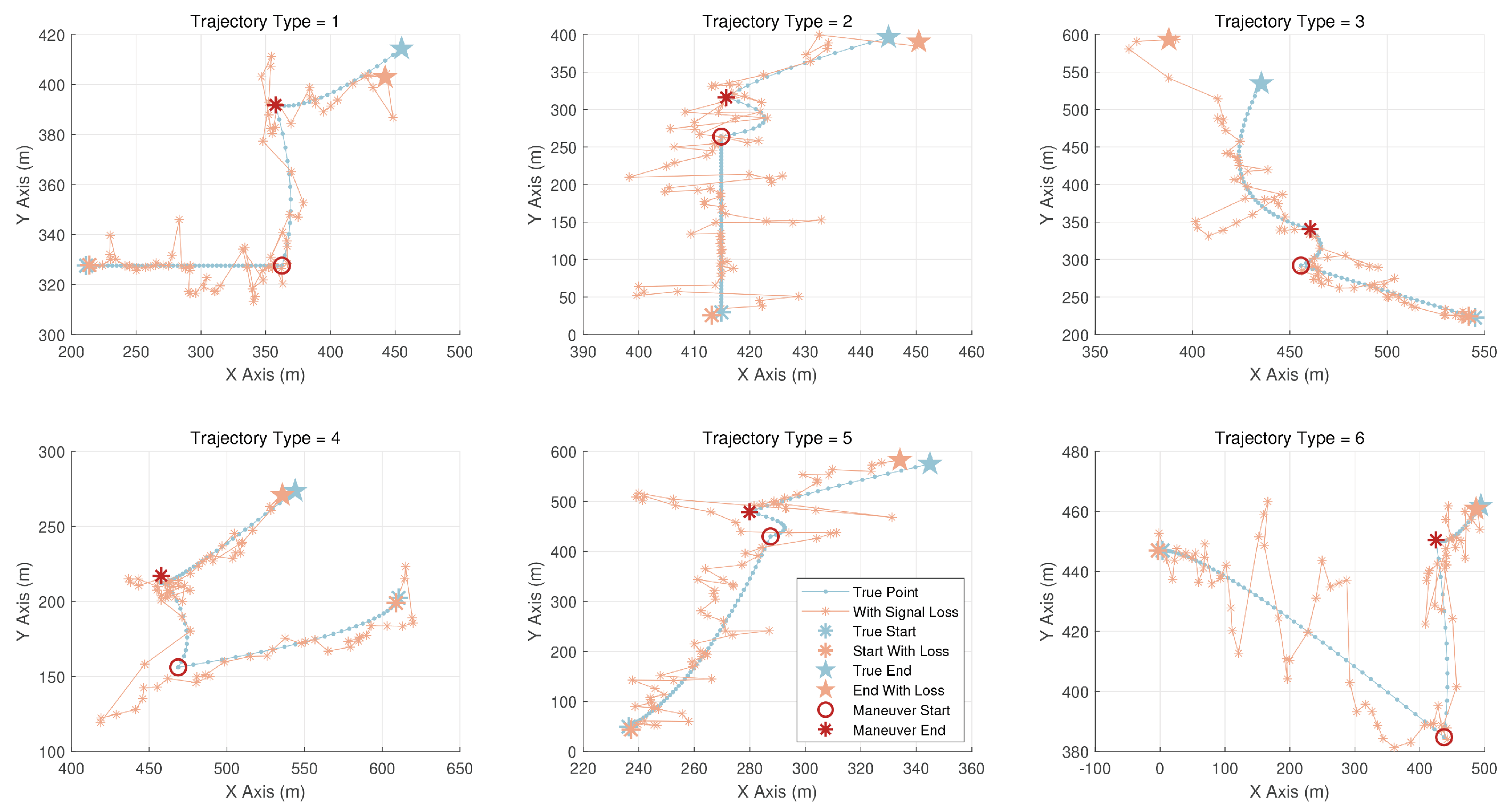
6.2.1. Trajectory Data

The simulation model generates a database of target movement trajectories, encompassing various movement types, as detailed in

Table 2. Trajectory types.

Type	Description
1	Lateral movement
2	Vertical movement
3	Diagonal movement (combining lateral and vertical speeds)
4	Curved movement with lateral acceleration
5	Curved movement with vertical acceleration
6	Complex curved movement with both lateral and vertical acceleration

.

Figure 13 illustrates the trajectories generated during the simulation, accompanied by random signal loss.

The motion of the AUV is divided into three distinct phases: the start phase, the maneuver phase, and the recovery phase. These phases are governed by a unified set of kinematic equations, adapted to each phase by adjusting the initial or boundary conditions. Let $\mathbf{p}\left(t\right)=\left[\begin{array}{c}x\left(t\right)\\ y\left(t\right)\end{array}\right]$, $\mathbf{v}\left(t\right)=\left[\begin{array}{c}{v}_x\left(t\right)\\ v_y\left(t\right)\end{array}\right]$, and $\mathbf{a}\left(t\right)=\left[\begin{array}{c}{a}_x\left(t\right)\\ a_y\left(t\right)\end{array}\right]$ denote the position, velocity, and acceleration of the AUV at time t, respectively. The unified kinematic equations are as follows:

$$\begin{array}{cc}\hfill \mathbf{p}\left(t\right)& =\mathbf{p}\left(t_{\mathrm{prev}}\right)+\mathbf{v}\left(t_{\mathrm{prev}}\right)·\Delta t+{\displaystyle \frac{1}{2}}\mathbf{a}\left(t_{\mathrm{prev}}\right)·{(\Delta t)}^2,\hfill \end{array}$$

(41)

$$\begin{array}{cc}\hfill \mathbf{v}\left(t\right)& =\mathbf{v}\left(t_{\mathrm{prev}}\right)+\mathbf{a}\left(t_{\mathrm{prev}}\right)·\Delta t,\hfill \end{array}$$

(42)

where $\Delta t=t-t_{\mathrm{prev}}$ represents the time step, and $t_{\mathrm{prev}}$ indicates the time at the beginning of the current phase.

In the start phase ($t\in [0,T_{\mathrm{start}})$), the AUV initializes its motion with specific starting conditions. The initial position, velocity, and acceleration are defined as $\mathbf{p}\left(t_{\mathrm{prev}}\right)={\mathbf{p}}_0=\left[\begin{array}{c}{x}_0\\ y_0\end{array}\right]$, $\mathbf{v}\left(t_{\mathrm{prev}}\right)={\mathbf{v}}_0=\left[\begin{array}{c}{v}_{x0}\\ v_{y0}\end{array}\right]$, and $\mathbf{a}\left(t_{\mathrm{prev}}\right)={\mathbf{a}}_0=\left[\begin{array}{c}{a}_{x0}\\ a_{y0}\end{array}\right]$, respectively. These parameters determine the initial state of the AUV, and the motion during this phase is described by the unified kinematic equations.

In the maneuver phase ($t\in [T_{\mathrm{start}},T_{\mathrm{maneuver}\_\mathrm{end}})$), the motion state undergoes abrupt changes. The acceleration $\mathbf{a}\left(t_{\mathrm{prev}}\right)$ and velocity $\mathbf{v}\left(t_{\mathrm{prev}}\right)$ are randomly selected from predefined distributions or ranges, denoted as ${\mathbf{a}}_{\mathrm{maneuver}}$ and ${\mathbf{v}}_{\mathrm{maneuver}}$, respectively, independent of the previous phase. The position $\mathbf{p}\left(t_{\mathrm{prev}}\right)$ is carried over from the end of the start phase, i.e., $\mathbf{p}\left(t_{\mathrm{prev}}\right)=\mathbf{p}\left(T_{\mathrm{start}}\right)$. This phase simulates abrupt maneuvers such as turning or changing direction, with both acceleration and velocity being randomly adjusted to reflect unpredictable changes in the AUV’s motion.

In the recovery phase ($t\in [T_{\mathrm{maneuver}\_\mathrm{end}},T_{\mathrm{measure}}]$), the acceleration and velocity are fine-tuned based on the initial phase’s final state. Specifically, the velocity $\mathbf{v}\left(t_{\mathrm{prev}}\right)$ is updated by adding a random perturbation $\Delta \mathbf{v}$ to the velocity at the end of the start phase:

$$\mathbf{v}\left(t_{\mathrm{prev}}\right)=\mathbf{v}\left(T_{\mathrm{start}}\right)+\Delta \mathbf{v},$$

(43)

where $\Delta \mathbf{v}$ is a random vector representing the velocity perturbation. The acceleration $\mathbf{a}\left(t_{\mathrm{prev}}\right)$ is updated by adding a random perturbation $\Delta \mathbf{a}\left(t\right)$ to the acceleration at the end of the start phase:

$$\mathbf{a}\left(t_{\mathrm{prev}}\right)=\mathbf{a}\left(T_{\mathrm{start}}\right)+\Delta \mathbf{a}\left(t\right),$$

(44)

where $\Delta \mathbf{a}\left(t\right)$ represents small random perturbations introduced to the acceleration. These perturbations decay over time as the AUV stabilizes its motion, i.e., $\Delta \mathbf{a}\left(t\right)\to \mathbf{0}$ as $t\to T_{\mathrm{measure}}$. This phase ensures that the AUV gradually returns to a stable motion trajectory after the abrupt maneuvers in the maneuver phase.

In summary, the motion of the AUV in each phase is governed by the same kinematic principles, with differences arising only in the initial or boundary conditions for each phase. In the start phase, the initial conditions are set; in the maneuver phase, the velocity and acceleration are randomly selected; and in the recovery phase, the velocity and acceleration are fine-tuned based on the initial phase’s final state, with small random perturbations decaying over time. This structure aligns with the previously discussed simulation of abrupt maneuvers.

As can be seen from Figure 13, when the traditional PF-TBD selects six different motion states in the start phase, there are substantial errors present, leading to a rather poor performance.

6.2.2. Feature Extraction at Each Time Step

For each trajectory, features are extracted at every time step to serve as inputs to the network, as depicted in Section 5.1.

6.2.3. Normalization and Dataset Preparation

After feature extraction, all features are normalized to ensure that the input data are consistent and well scaled. Normalization is particularly important when dealing with features that have different units or ranges, such as velocity (m/s) and position (meters). The normalization process follows the equation

$$x_{\mathrm{norm}}={\displaystyle \frac{x-\mu }{\sigma }},$$

(45)

where x is the original feature value, $\mu$ is the mean, and $\sigma$ is the standard deviation.

The normalized features are then packaged into a dataset. Each sample in the dataset includes the following:

• Input: A sequence of time steps, where each step contains a feature vector that includes information such as position, velocity, acceleration, and likelihood values.
• Output: The predicted error in the x and y coordinates at the corresponding time step allows the network to learn temporal dependencies and predict localization errors over time.

The dataset is divided into training, validation, and test sets to evaluate the model performance across different conditions. The network is trained on the training set, with its performance validated on the validation set and tested on the test set.

6.3. Experimental Evaluation Indicators

To evaluate the performance of the models, common regression metrics including mean absolute error (MAE), mean absolute percentage error (MAPE), mean squared error (MSE), root mean squared error (RMSE), and coefficient of determination ($R^2$) are employed.

The mean absolute error (MAE) measures the average magnitude of the errors in predictions, calculated as

$$\mathrm{MAE}={\displaystyle \frac{1}{n}}\sum _{i=1}^n|y_i-{\widehat{y}}_i|,$$

(46)

where $y_i$ represents the ground truth values, ${\widehat{y}}_i$ the predicted values, and n is the total number of samples.

The mean absolute percentage error (MAPE) is another common metric that evaluates the prediction error in percentage terms, defined by

$$\mathrm{MAPE}={\displaystyle \frac{100\%}{n}}\sum _{i=1}^n\left|{\displaystyle \frac{y_i-{\widehat{y}}_i}{y_i}}\right|.$$

(47)

The mean squared error (MSE) emphasizes larger errors by squaring them, thus penalizing outliers. It is expressed as

$$\mathrm{MSE}={\displaystyle \frac{1}{n}}\sum _{i=1}^n{(y_i-{\widehat{y}}_i)}^2.$$

(48)

Based on MSE, the root mean squared error (RMSE) provides a measure of error in the same units as the output variable, calculated as

$$\mathrm{RMSE}=\sqrt{{\displaystyle \frac{1}{n}}\sum _{i=1}^n{(y_i-{\widehat{y}}_i)}^2}.$$

(49)

The coefficient of determination, denoted as $R^2$, provides a measure of how well the model explains the variance in the actual data values. Specifically, $R^2$ is defined as

$$R^2=1-{\displaystyle \frac{{\sum }_{i=1}^n{(y_i-{\widehat{y}}_i)}^2}{{\sum }_{i=1}^n{(y_i-\overline{y})}^2}}$$

(50)

where $\overline{y}$ denotes the mean of the actual values $y_i$. An $R^2$ value closer to 1 indicates that the model accounts for a larger proportion of the variance in the actual data, which indicates a stronger fit to the data.

6.4. Result

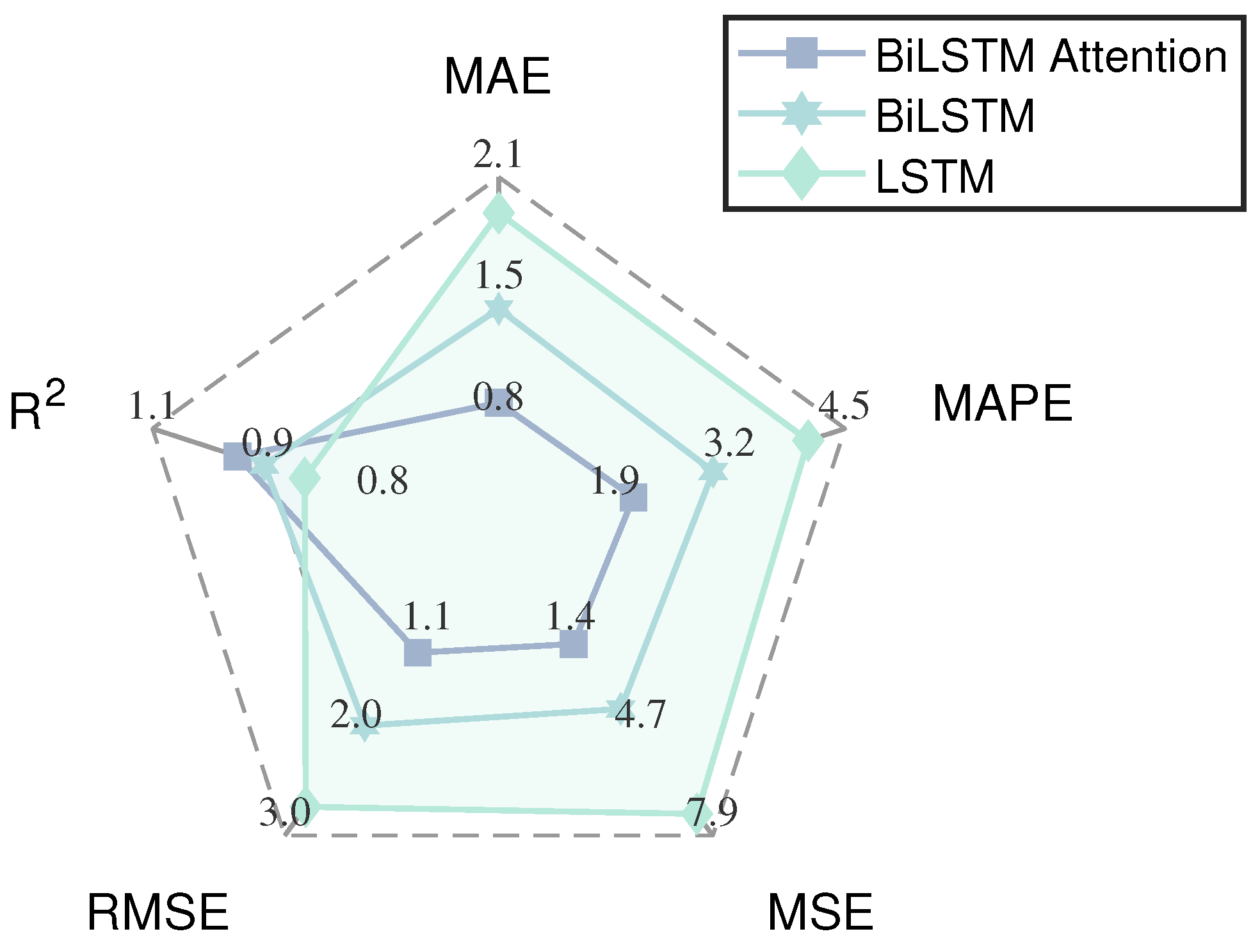
6.4.1. Performance Comparison

Table 3. Model performance comparison.

Metric	BiLSTM-Attention			BiLSTM			LSTM
	Training	Validation	Test	Training	Validation	Test	Training	Validation	Test
MAE	0.72368	0.88564	0.90614	1.0043	1.4121	1.4079	1.419	1.9544	1.919
MAPE	2.8529	4.2637	2.1524	3.8393	7.1145	3.0427	4.6777	8.5696	4.1049
MSE	0.90529	1.439	1.5599	1.7915	3.8673	3.7198	3.7154	7.6711	7.211
RMSE	0.95147	1.1996	1.249	1.3385	1.9666	1.9287	1.9275	2.7697	2.6853
$R^2$	0.98869	0.98145	0.98298	0.97657	0.94615	0.95219	0.9507	0.89159	0.90554

Performance metrics for different models on training, validation, and test sets.

presents a comparative analysis of the BiLSTM-Attention, BiLSTM, and LSTM models across multiple performance metrics. In particular, both the BiLSTM-Attention and the BiLSTM models outperform the standard LSTM, with the BiLSTM’s bidirectional structure allowing it to capture sequence dependencies with greater fidelity. This bidirectional approach enriches the model’s understanding of sequential data, enhancing its ability to grasp intricate patterns that might otherwise remain obscured in a unidirectional framework.

As illustrated in Figure 14, the BiLSTM-Attention model exhibits a significant reduction in prediction error, achieving a mean absolute error (MAE) of 0.90614 on the test set. This is considerably lower than that of LSTM (MAE = 1.919) and BiLSTM (MAE = 1.4079). Additionally, the mean square error (MSE) reinforces these findings, with BiLSTM-Attention attaining an MSE of 1.5599, in stark contrast to the MSE values of 3.7198 for BiLSTM and 7.211 for LSTM.

The effectiveness of BiLSTM-Attention stems from its dual strengths: BiLSTM enhances the model’s ability to retain contextual information from both past and future states, while the multi-head attention layer selectively amplifies the most relevant features from various perspectives within this context. This selective amplification not only reduces the impact of noise, but also allows the model to dynamically recalibrate its focus in response to changing input patterns, a critical feature in applications characterized by high variability and complex temporal dependencies.

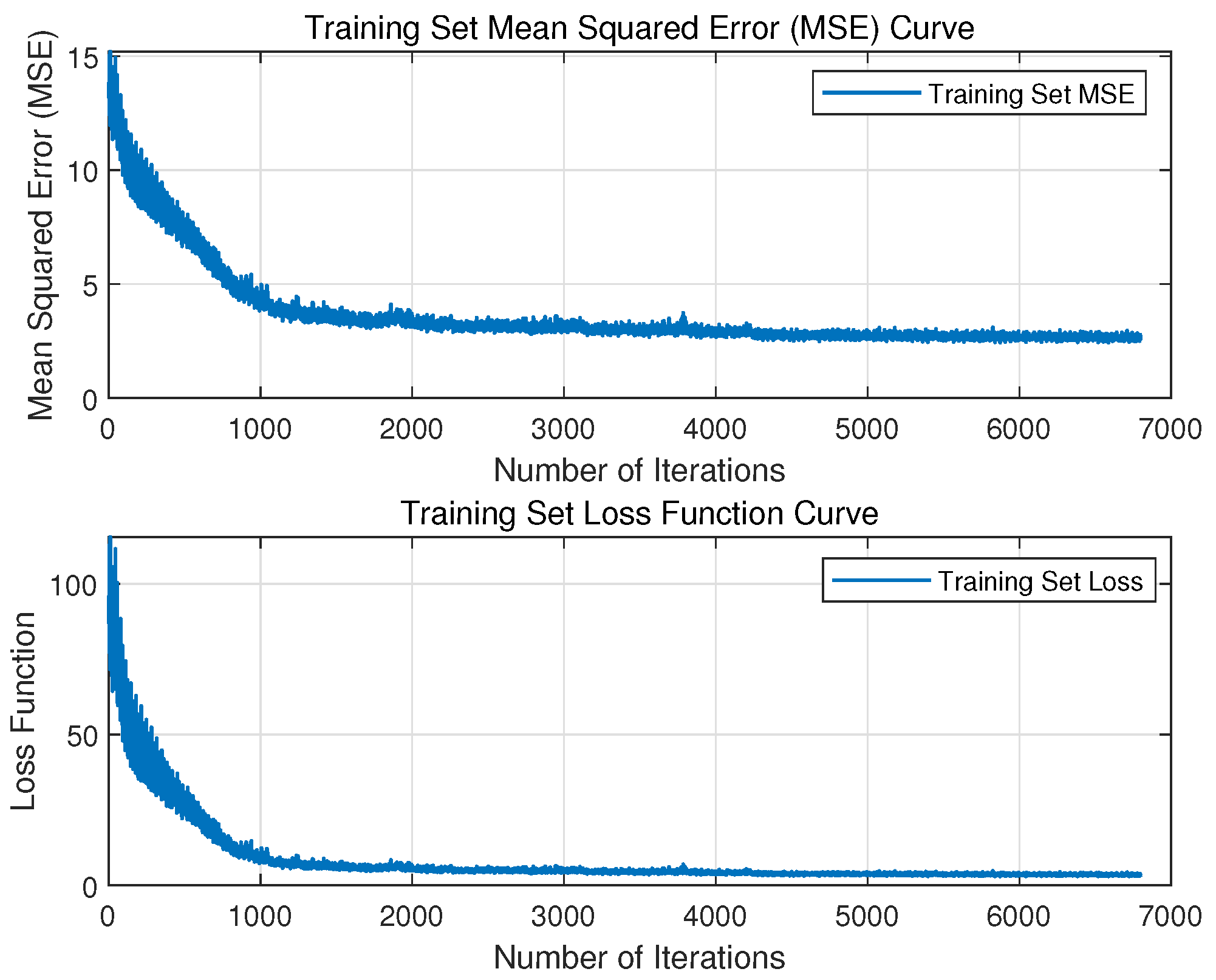
6.4.2. Training Loss and RMSE

The BiLSTM-Attention model was trained over 6000 iterations. Figure 15 shows both the training loss and the root mean squared error (RMSE) recorded at each iteration, providing insight into the model’s improvement in estimation accuracy over time.

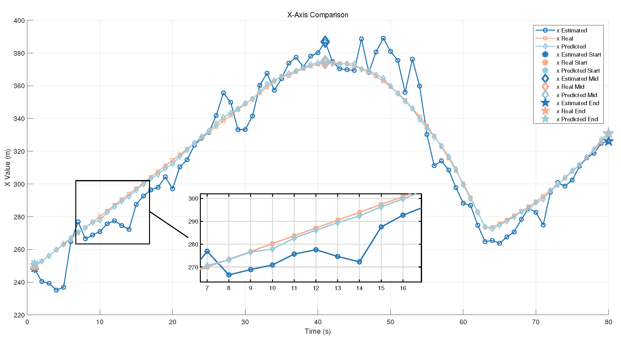
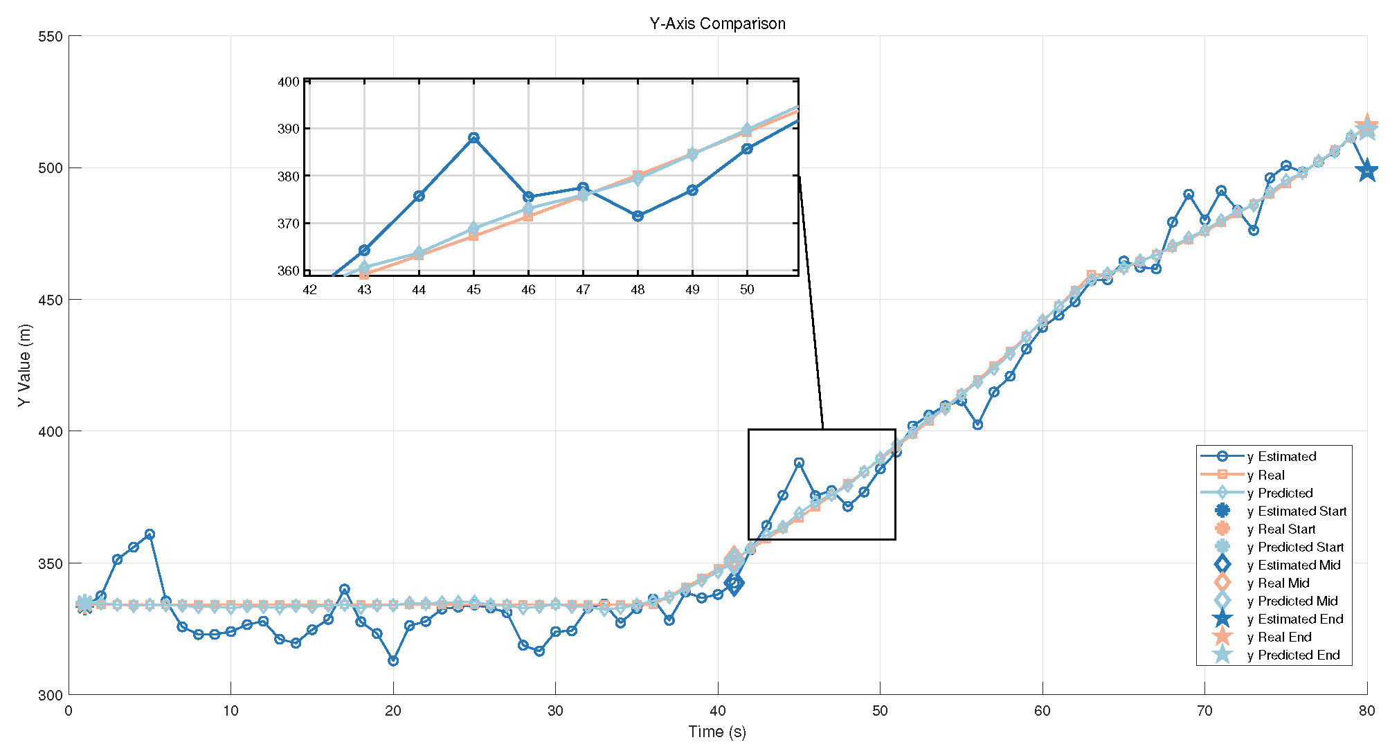
6.4.3. Position Estimation Error

For clarity in the following discussion, we define three terms: the position estimates obtained using the BiLSTM-Attention-PFTBD algorithm are referred to as Predicted Position; the estimates derived solely from the traditional PFTBD algorithm are referred to as Estimated Position; and the actual coordinates of the target are referred to as Real Position.

Figure 16, Figure 17 and Figure 18 show the position estimation errors along the X and Y coordinates, as well as the combined X and Y errors. The results demonstrate that the BiLSTM-Attention model significantly improves position estimates compared to the traditional PFTBD algorithm, confirming its superior performance in enhancing tracking accuracy.

The corresponding midpoints in these three graphs, marked with diamonds, can be used for comparative analysis, allowing observation of their variations along the X and Y axes. This facilitates the comparison of features at the same positions across different graphs.

7. Conclusions and Discussion

This paper presents the BiLSTM-Attention-PFTBD algorithm, a novel approach combining bidirectional Long Short-Term Memory (BiLSTM) networks and multi-head attention within the particle filter Track-Before-Detect (PFTBD) framework, aimed at improving tracking in long-baseline acoustic localization (LBL) systems. This algorithm addresses the challenges faced by AUVs in complex, adversarial environments, such as abrupt maneuvers and interference from non-cooperative sources.

The BiLSTM component captures both past and future temporal dependencies, enabling the model to adapt to sudden motion changes and environmental conditions. The multi-head attention mechanism allows the model to focus on multiple aspects of the input data, improving pattern recognition and tracking accuracy. This is particularly useful for AUV underwater localization, where precise tracking is essential in dynamic, hostile environments.

Simulation results demonstrate that the BiLSTM-Attention-PFTBD algorithm outperforms traditional methods, offering better localization accuracy and robustness, even in the presence of interference and unpredictable AUV movements. The algorithm ensures stable tracking in challenging conditions, highlighting its potential for high-risk missions where precise localization is crucial.

To extend BiLSTM-Attention-PFTBD for multi-target tracking, modifications are necessary. The network should independently process features from multiple targets, incorporate a target identification module, and expand the attention mechanism to focus on multiple targets, among others.

Future research should investigate these adaptations to effectively support multi-target tracking. In addition, although our method shows promising results, its performance with real-world TOA/TDOA data remains to be validated. In future work, we aim to collaborate with relevant laboratories or institutions to acquire real measurement data. This will allow us to further validate and refine our method, enhancing its credibility and practical applicability in real-world scenarios.

References

1. Lv, P.-F.; Guo, J.; Lv, J.-Y.; He, B. Integrated Navigation of Autonomous Underwater Vehicle Based on HG-RNN and EKF. In Proceedings of the OCEANS 2024, Singapore, 15–18 April 2024; pp. 1–5. [Google Scholar] [CrossRef]
2. Zhao, W.; Zhao, S.; Liu, G.; Meng, W. Range-Only Single Beacon Based Multisensor Fusion Positioning for AUV. IEEE Sens. J. 2023, 23, 23399–23409. [Google Scholar] [CrossRef]
3. Paull, L.; Saeedi, S.; Seto, M.; Li, H. AUV navigation and localization: A review. IEEE J. Ocean. Eng. 2014, 39, 131–149. [Google Scholar] [CrossRef]
4. Li, J.; Wang, T. Underwater Localization Techniques. Underw. Acoust. J. 2023, 18, 88–97. [Google Scholar]
5. Aditya, R.; Balasubramanian, S. Survey of underwater acoustic localization methods. Ocean Eng. 2018, 20, 105–117. [Google Scholar]
6. Morelande, M.; Ristic, B. Signal-to-noise ratio threshold effect in track before detect. IET Radar Sonar Navig. 2009, 3, 601–608. [Google Scholar] [CrossRef]
7. Fang, Q.; Wang, X. Non-cooperative MPSK modulation detection using machine learning techniques. In Proceedings of the 2021 IEEE International Conference on Communications, Montreal, QC, Canada, 14–18 June 2021; pp. 1–5. [Google Scholar]
8. Wang, Y.; Yan, H.; Pan, C.; Liu, S. Measurement-Based Analysis of Characteristics of Fast Moving Underwater Acoustic Communication Channel. In Proceedings of the 2022 International Conference on Frontiers of Information Technology (FIT), Islamabad, Pakistan, 12–13 December 2022; pp. 47–52. [Google Scholar] [CrossRef]
9. Wang, J.; Cai, P.; Yuan, D. An Underwater Acoustic Channel Simulator for UUV Communication Performance Testing. In Proceedings of the 2010 IEEE International Conference on Information and Automation, Harbin, China, 20–23 June 2010; pp. 2286–2290. [Google Scholar] [CrossRef]
10. Coskun, A.; Kale, I. Blind Multidimensional Matched Filtering Techniques for Single Input Multiple Output Communications. IEEE Trans. Instrum. Meas. 2010, 59, 1056–1064. [Google Scholar] [CrossRef]
11. Hamidi, E.; Weiner, A.M. Phase-Only Matched Filtering of Ultrawideband Arbitrary Microwave Waveforms via Optical Pulse Shaping. J. Light. Technol. 2008, 26, 2355–2363. [Google Scholar] [CrossRef]
12. Daffalla, M.M. Adaptive multifunction filter for radar signal processing. In Proceedings of the 2013 International Conference on Computing, Electrical and Electronic Engineering (ICCEEE), Khartoum, Sudan, 26–28 August 2013; pp. 35–39. [Google Scholar] [CrossRef]
13. Naus, K.; Piskur, P. Applying the Geodetic Adjustment Method for Positioning in Relation to the Swarm Leader of Underwater Vehicles Based on Course, Speed, and Distance Measurements. Energies 2022, 15, 8472. [Google Scholar] [CrossRef]
14. Bi, X.; Du, J.; Zhang, Q.; Wang, W. Improved Multi-Target Radar TBD Algorithm. J. Syst. Eng. Electron. 2015, 26, 1229–1235. [Google Scholar] [CrossRef]
15. Aharonovich, I.; Bray, K.; Shimoni, O. Florescent Nanodiamonds for Biomedical Applications. In Proceedings of the 2016 Conference on Lasers and Electro-Optics (CLEO), San Jose, CA, USA, 5–10 June 2016; p. 1. [Google Scholar]
16. Li, H.; Zhang, Z. Long-baseline navigation with multi-model particle filters. In Proceedings of the IEEE Oceans Conference, Seattle, WA, USA, 27–31 October 2019; pp. 300–305. [Google Scholar]
17. Pan, H.; Zhang, L. Impact of time synchronization attacks on underwater sensor networks. IEEE Trans. Sens. Netw. 2022, 21, 1213–1222. [Google Scholar]
18. Smith, A.; Doe, J. Obstacle avoidance in autonomous underwater vehicles: A review. Electronics 2021, 11, 2301. [Google Scholar]
19. Liu, C.; Lv, Z.; Xiao, L.; Su, W.; Ye, L.; Yang, H.; You, X.; Han, S. Efficient Beacon-Aided AUV Localization: A Reinforcement Learning Based Approach. IEEE Trans. Veh. Technol. 2024, 73, 7799–7811. [Google Scholar] [CrossRef]
20. Stefanidou, A.; Politi, E.; Chronis, C.; Dimitrakopoulos, G.; Varlamis, I. A Deep Reinforcement Learning Approach for Navigation and Control of Autonomous Underwater Vehicles in Complex Environments. In Proceedings of the 2024 18th International Conference on Control, Automation, Robotics and Vision (ICARCV), Dubai, United Arab Emirates, 12–15 December 2024; pp. 750–755. [Google Scholar] [CrossRef]
21. Yao, J.; Yang, J.; Zhang, C.; Zhang, J.; Zhang, T. Autonomous Underwater Vehicle Trajectory Prediction with the Nonlinear Kepler Optimization Algorithm–Bidirectional Long Short-Term Memory–Time-Variable Attention Model. J. Mar. Sci. Eng. 2024, 12, 1115. [Google Scholar] [CrossRef]
22. Li, C.; Hu, Z.; Zhang, D.; Wang, X. System Identification and Navigation of an Underactuated Underwater Vehicle Based on LSTM. J. Mar. Sci. Eng. 2025, 13, 276. [Google Scholar] [CrossRef]
23. Li, X.; Wang, Y.; Qi, B.; Hao, Y. Long Baseline Acoustic Localization Based on Track-Before-Detect in Complex Underwater Environments. IEEE Trans. Geosci. Remote Sens. 2023, 61, 1–14. [Google Scholar] [CrossRef]
24. Bar-Shalom, Y.; Fortmann, T. Target Tracking: A Bayesian Approach; Springer: Berlin/Heidelberg, Germany, 1988. [Google Scholar]
25. Maskell, S.; Gordon, N. A tutorial on particle filters for online nonlinear/non-Gaussian Bayesian tracking. Proc. IEEE 2002, 92, 401–422. [Google Scholar]
26. Michaels, J.E.; Michaels, T.E. Detection of sudden target maneuvers in particle filters. IEEE Trans. Aerosp. Electron. Syst. 2008, 44, 1075–1091. [Google Scholar]
27. Ma, X.; Karkus, P.; Hsu, D.; Lee, W.S. Particle Filter Recurrent Neural Networks. arXiv 1905. [Google Scholar] [CrossRef]
28. Wang, Y.; Wang, H.; Li, Q.; Xiao, Y.; Ban, X. Passive Sonar Target Tracking Based on Deep Learning. J. Mar. Sci. Eng. 2022, 10, 181. [Google Scholar] [CrossRef]
Figure 1. Comparison of true and PF-TBD-estimated trajectories during abrupt maneuver transitions. Errors occur at maneuver start and end points, revealing PF limitations.
Drones 09 00204 g001
Figure 2. Trajectory estimation errors due to signal jamming, showing the differences between predicted trajectories with and without signal loss compared to the true trajectory. The inset provides a closer look at the performance under normal conditions (without signal loss), where the predicted trajectory closely aligns with the true trajectory, demonstrating the reliability of the base algorithm in normal environments. However, when signal loss occurs, the predicted trajectory deviates significantly from the true trajectory, emphasizing the necessity and rationality of extending PF-TBD to adversarial environments.
Drones 09 00204 g002
Figure 3. Trajectory estimation errors under full−band jamming.
Drones 09 00204 g003
Figure 4. Illustration of tracking performance under maneuvering and signal loss conditions.
Drones 09 00204 g004
Figure 5. Structure of an LSTM cell.
Drones 09 00204 g005
Figure 6. Structure of BiLSTM networks.
Drones 09 00204 g006
Figure 7. Attention mechanism.
Drones 09 00204 g007
Figure 8. Multi-head attention mechanism.
Drones 09 00204 g008
Figure 9. The overall architecture of the proposed algorithm and the training process. The BiLSTM-Attention network model is represented by the network block, which will be explained in detail later. The output of the network module, which includes Xerror and Yerror, is used to calculate the loss. This loss is then used to adjust the parameters through backpropagation, thereby improving the model’s performance.
Drones 09 00204 g009
Figure 10. An example illustrating feature extraction for TOA alignment. Here, “index” refers to a position within this 2000−point signal array. The red symbol indicates the Predicted Index, which shows a substantial deviation from the Real Index marked in green. In contrast, the Find peak, marked in blue, closely matches the true TOA, demonstrating its potential as a corrective feature for more accurate TOA estimation in particle filtering.
Drones 09 00204 g010
Figure 11. BiLSTM-Attention model architecture. Forward and backward LSTM layers process the input sequence, and their outputs are concatenated before passing through an attention layer. The attention-weighted output is used to predict future localization errors.
Drones 09 00204 g011
Figure 12. Diagram of the LBL system in adversarial environments.
Drones 09 00204 g012
Figure 13. Trajectories of different types along with the corresponding performance of the PF−TBD estimated results.
Drones 09 00204 g013
Figure 14. Performance comparison of BiLSTM-Attention, BiLSTM, and LSTM models on the test set.
Drones 09 00204 g014
Figure 15. Training loss and RMSE over 6000 iterations. Top: RMSE for position estimates. Bottom: Training loss.
Drones 09 00204 g015
Figure 16. Comparison of estimated, predicted, and real positions of target over time in X-coordinate.
Drones 09 00204 g016
Figure 17. Comparison of estimated, predicted, and real positions of target over time in Y-coordinate.
Drones 09 00204 g017
Figure 18. Combined X and Y coordinate error estimation for BiLSTM-Attention model, showing improved tracking accuracy.
Drones 09 00204 g018