Assessing Seasonal and Diurnal Thermal Dynamics of Water Channel and Highway Bridges Using Unmanned Aerial Vehicle Thermography

Abstract

Bridges are critical components of modern infrastructure, yet their long-term performance is often compromised by thermal stresses induced by environmental and material factors. Despite advances in remote sensing, characterizing the complex thermal dynamics of bridge structures remains challenging. In this study, we investigate the seasonal and diurnal thermal behavior of two common bridge types—a water channel bridge with paving stone surfacing and a highway bridge with asphalt surfacing—using high-resolution UAV thermography. A pre-designed photogrammetric flight plan (yielding a ground sampling distance of <5 cm) was implemented to acquire thermal and visual imagery during four distinct temporal windows (winter morning, winter evening, summer morning, and summer evening). The methodology involved generating thermal orthophotos via structure-from-motion techniques, extracting systematic temperature measurements ($n=150$ per bridge), and analyzing these using independent-samples and paired t-tests to quantify material-specific thermal responses and environmental coupling effects. The results reveal that the water channel bridge exhibited significantly lower thermal variability (1.54–3.48 °C) compared to the highway bridge (3.27–5.66 °C), with pronounced differences during winter mornings (Cohen’s $d=2.03$, $p<0.001$). Furthermore, material properties strongly modulated thermal dynamics, as evidenced by the significant temperature differentials between the paving stone and asphalt surfaces, while ambient conditions further influence surface–ambient coupling ($r=0.961$ vs. $0.975$). The results provide UAV-based quantitative metrics for bridge thermal assessment and empirical evidence to support the temporal monitoring of bridges with varying materials and environmental conditions for future studies.

1. Introduction

Bridge infrastructure represents a critical component of modern transportation networks, requiring continuous monitoring and maintenance to ensure structural integrity and public safety [1]. The long-term performance of these structures is governed by complex interactions between environmental conditions, material properties, and mechanical loads, with thermal behavior emerging as a particularly crucial yet often underappreciated determinant of structural health [2]. Temperature-induced stresses and deformations can significantly impact both immediate structural responses and long-term deterioration patterns, necessitating sophisticated approaches to thermal assessment and monitoring [3].

The challenges of understanding bridge thermal dynamics have grown increasingly complex as infrastructure ages and climate patterns have evolved [4]. Traditional structural health monitoring approaches, primarily focused on mechanical responses and visible deterioration, often fail to capture the subtle yet significant impacts of thermal behavior on structural performance. These thermal effects manifest through multiple mechanisms, including differential expansion and contraction, thermal gradients inducing internal stresses, and temperature-dependent material property variations [5]. The cumulative impact of these thermal phenomena can accelerate deterioration processes, affect load-carrying capacity, and influence maintenance requirements, highlighting the critical importance of comprehensive thermal assessment in bridge management strategies [6].

Recent technological developments, particularly in remote sensing and data processing, have significantly enhanced our ability to study bridge thermal behavior. While traditional point-based temperature measurements offer a narrow perspective, modern assessment methods allow for a comprehensive examination of thermal patterns across entire structures [7]. This improvement in assessment capabilities has highlighted the complexity of bridge thermal responses and their significant implications for structural health monitoring and maintenance planning [8].

The development of thermal assessment methods has led to a systematic increase in bridge structural monitoring capabilities. Early foundational work by Zuk [9] and Wah and Kirksey [10] established fundamental principles through static temperature distributions and basic thermal characteristics using fixed sensor networks. Although constrained by technological limitations, this initial research provided an essential understanding of thermal impacts on structural performance. Subsequent investigations by Fu et al. [11] and Chang and Im [12] expanded the field by conducting more sophisticated studies on composite bridge structures, demonstrating critical relationships between thermal effects and structural durability.

A significant development emerged through long-term monitoring studies in the early 2000s, fundamentally altering our understanding of thermal impacts. Research by Liu et al. [13] showed that temperature-induced deformations could substantially exceed traffic-induced stresses, particularly in regions experiencing extreme temperature variations. The impact of thermal loading was further demonstrated by Yang et al. [14] through detailed monitoring of a cable-stayed bridge. They established strong linear relationships between temperature variations and tower displacements, documenting how thermal actions substantially influence quasi-static structural responses and cable forces. Burdet’s [3] comprehensive analysis quantified this phenomenon, demonstrating that thermal effects could account for up to 60% of observed structural deformations, highlighting thermal behavior as a critical parameter in structural assessment and maintenance planning.

Modern bridge thermal assessment has transcended traditional point measurement limitations through integrated technological approaches. While fixed sensor networks provide continuous temporal data, their discrete nature often fails to capture the complex spatial distributions of thermal gradients crucial for identifying structural anomalies [15,16]. Recent developments have addressed these limitations through comprehensive monitoring systems that capture both spatial and temporal variations in thermal behavior [2,17]. The integration of advanced technologies has enabled sophisticated multi-modal assessment capabilities, including the combination of InSAR and LiDAR for comprehensive structural assessment [18,19] and the application of deep learning algorithms for thermal anomaly classification [20].

Among these advancements, thermal imaging technologies, particularly when integrated with Unmanned Aerial Vehicle (UAV) systems, have played a transformative role in bridge inspection capabilities. Recent developments in UAV technology, coupled with enhanced sensor integration, have greatly broadened the scope of aerial applications. In particular, thermal imaging platforms mounted on UAVs offer exceptional spatial resolution, operational agility, and cost efficiency. These attributes have paved the way for their deployment across a variety of disciplines—from agricultural monitoring [21,22,23] and evaporation analysis [24] to archaeological investigations [25], assessments of building energy performance [26], the monitoring of land cover types [27,28,29,30,31,32], and detection of urban heat islands [33,34,35]. Within the context of bridge inspection, Omar and Nehdi [36] demonstrated the efficacy of UAV thermography for concrete bridge deck inspection, achieving detection accuracies exceeding 85% for subsurface delaminations. This capability has been further enhanced through automated analysis protocols [37] and 360-degree inspection methodologies [38], significantly improving assessment comprehensiveness.

Recent research has developed advanced methodologies for understanding material-specific thermal responses and environmental modulation effects. Studies by Mariani et al. [39] demonstrated that material-specific thermal responses significantly influence both short-term temperature distributions and long-term structural performance, building on the thermal pattern identification work by Truong et al. [40]. Moreover, researchers have developed refined protocols accounting for material variations in thermal assessment procedures [41,42], improving the accuracy of structural evaluations. Additionally, environmental context has emerged as a crucial modulator of bridge thermal behavior. Research by Biscarini et al. [43] documented the significant influences of water bodies on bridge thermal characteristics exerted through enhanced convective cooling and humidity variations. Research on harsh environmental conditions has expanded this perspective [44], contributing to comprehensive infrastructure asset management strategies [45].

Despite significant advances in bridge thermal assessment methods, several critical knowledge gaps persist that warrant systematic investigation. Although recent studies have demonstrated the effectiveness of UAV-based thermal imaging for structural assessment, quantitative methods for analyzing high-resolution thermal data—especially in bridges across diverse environmental conditions—remain insufficiently developed. The interpretation of spatial thermal patterns and their relationship to structural health requires more sophisticated analytical approaches that can account for environmental variability and material-specific responses. Given that highway and water channel bridges are among the most commonly encountered bridge types, understanding how they respond to varying environmental conditions remains a critical area for further investigation.

Understanding how environmental factors influence thermal behavior in water channel and highway bridges requires further investigation, as the existing research primarily focuses on isolated structural contexts without comprehensive comparative analysis. This gap is particularly significant given the diverse environmental conditions bridges experience and their potential impact on maintenance requirements and structural longevity. Furthermore, integrating material-specific thermal response analysis into maintenance planning strategies requires further methodological development, with new approaches needed to translate thermal behavior patterns into practical maintenance guidelines. To address these gaps, this study analyzes thermal data collected via UAV-based imaging for two bridge types—a water channel bridge with paving stone surfacing and a highway bridge with asphalt surfacing—across seasonal (summer/winter) and diurnal (morning/evening) cycles. The results aim to provide a comprehensive understanding of seasonal and diurnal thermal variations and their implications for structural assessment and maintenance planning.

In this study, four fundamental research questions are explored to better our understanding of bridge thermal dynamics: [RQ1] How do spatial temperature distributions differ between water channel and highway bridges across seasonal and diurnal cycles? [RQ2] What are the quantitative relationships between environmental factors and bridge thermal dynamics? [RQ3] What are the material-specific thermal responses of bridges? [RQ4] Can statistical methods and UAV thermography effectively identify and characterize significant thermal patterns?

The remainder of this paper is organized to systematically present the research methodology, findings, and implications. Section 2 describes the methodology, including data acquisition protocols, processing procedures, and analytical approaches. Section 3 presents comprehensive results of seasonal and diurnal thermal analyses, featuring statistical characterization of thermal patterns, comparative analysis between bridge types, and material-specific thermal responses. Section 4 discusses the broader implications of these findings for bridge monitoring and maintenance practices, while Section 5 concludes with specific recommendations for implementation and future research directions.

2. Materials and Methods

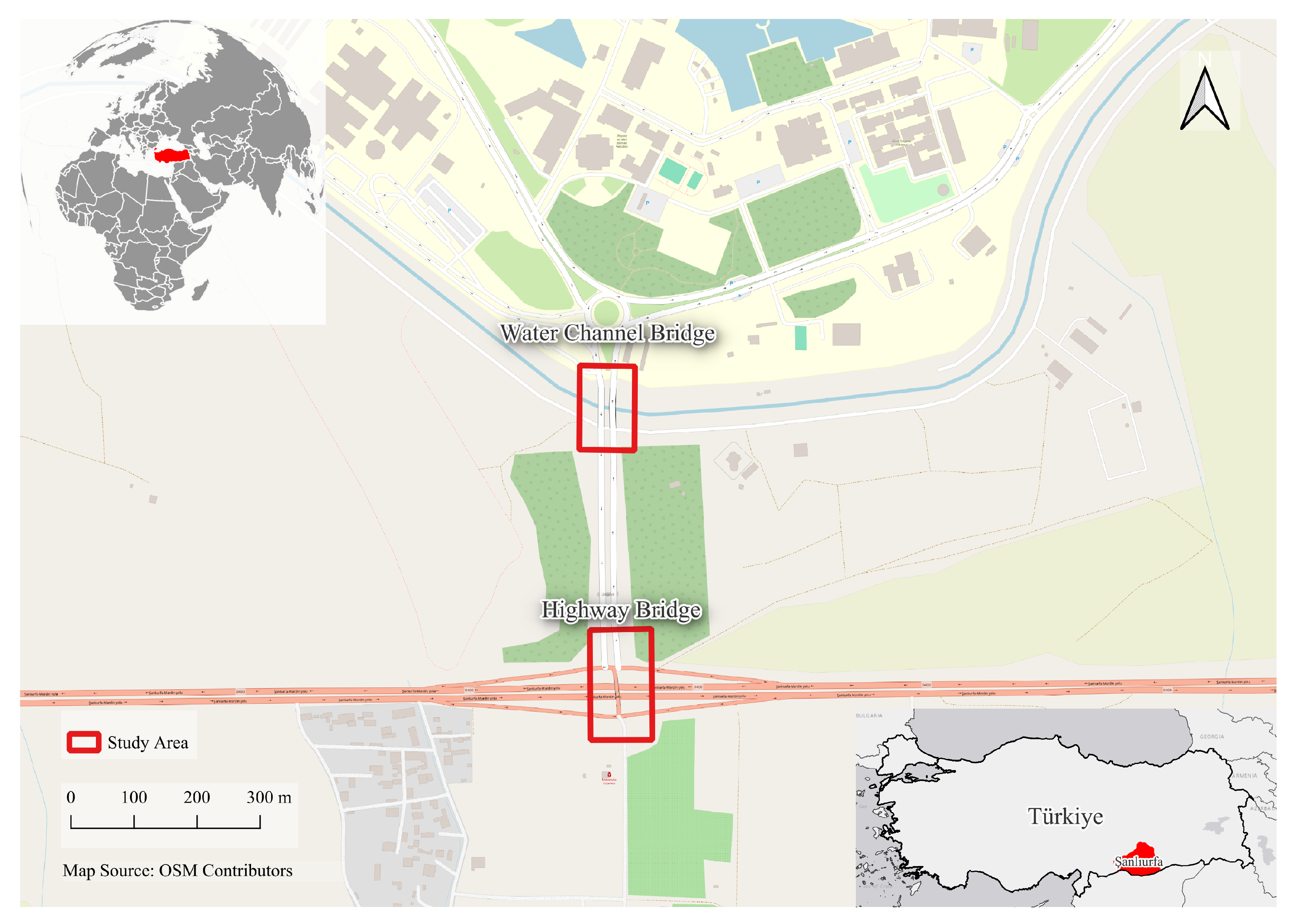
2.1. Study Area

The research was conducted at Harran University’s Osmanbey Campus, located in Şanlıurfa Province, southeastern Türkiye, in a semi-arid region characterized by hot, dry summers and mild winters. The study focused on two characteristic bridges within the campus infrastructure network: a water channel bridge and a highway bridge, separated by approximately 300 m along a north–south axis (Figure 1).

The water channel bridge, positioned at the northern extent of the study area, spans an engineered waterway that serves as an irrigation channel. This reinforced concrete structure is situated within a mixed-use campus zone bordered by institutional buildings to the north and open spaces to the south. The water channel bridge, extending 41 m in length and spanning 35.5 m in width, features a reinforced concrete deck with paving stone surface treatment and maintains a vertical clearance of 2.40 m from the water surface to the bridge surface.

The highway bridge, located approximately 300 m south of the water channel bridge, crosses a major transportation corridor. This reinforced concrete structure, measuring 48.6 m in length and 12.3 m in width, incorporates an asphalt surface material over its concrete deck and features a 7 m vertical clearance between the underlying road surface and bridge surface. The bridge is situated in an urban environment and subject to heavy traffic loads.

The study area within Osmanbey Campus provided a controlled environment for comparative analysis as both bridges experience similar macroclimatic conditions while maintaining distinct microenvironmental characteristics. The selection of these specific bridge locations allowed for the investigation of how different environmental contexts—specifically water proximity and high traffic density—influence structural thermal dynamics.

2.2. Data Acquisition

Data acquisition was conducted using a DJI Mavic 3E Thermal quadcopter UAV equipped with a dual-camera payload system [46]. The primary thermal sensor consisted of a radiometric thermal camera utilizing a 640 × 512 pixel microbolometer array with a 40 mm lens (DFOV: 61°). The thermal imager operates in the long-wave infrared spectral range (8–14 μm) with a noise equivalent temperature difference, enabling high-fidelity temperature measurements across a detection range of −20 °C to 150 °C. Temperature measurement accuracy was maintained at ±2 °C or for ±2% of the reading, whichever was greater. While this level of accuracy is robust, our study primarily emphasizes relative temperature differences rather than absolute temperature values; consequently, minor deviations in absolute temperature do not affect the validity of our conclusions.

The system’s complementary RGB camera, featuring a 4/3 CMOS sensor with a mechanical shutter, provided concurrent visual imagery at 20 MP resolution (5280 × 3956 pixels). This dual-sensor configuration enabled precise spatial correlation between thermal and visual data during post-processing.

The UAV was operated at an altitude of 30 m above ground level, yielding a ground sampling distance (GSD) of 4.98 cm/pixel for thermal imagery and 1.44 cm/pixel for RGB orthomosaic data. Data collection flights followed pre-designed routes with 80% forward overlap and 80% side overlap between adjacent flight lines, ensuring complete coverage and facilitating accurate photogrammetric processing. Ambient temperature was recorded using a portable weather station positioned near the bridge sites during each flight. Environmental factors such as humidity, wind speed, and general temperature changes were assumed to be equal and constant, as both bridges are in close proximity, ensuring similar meteorological conditions.

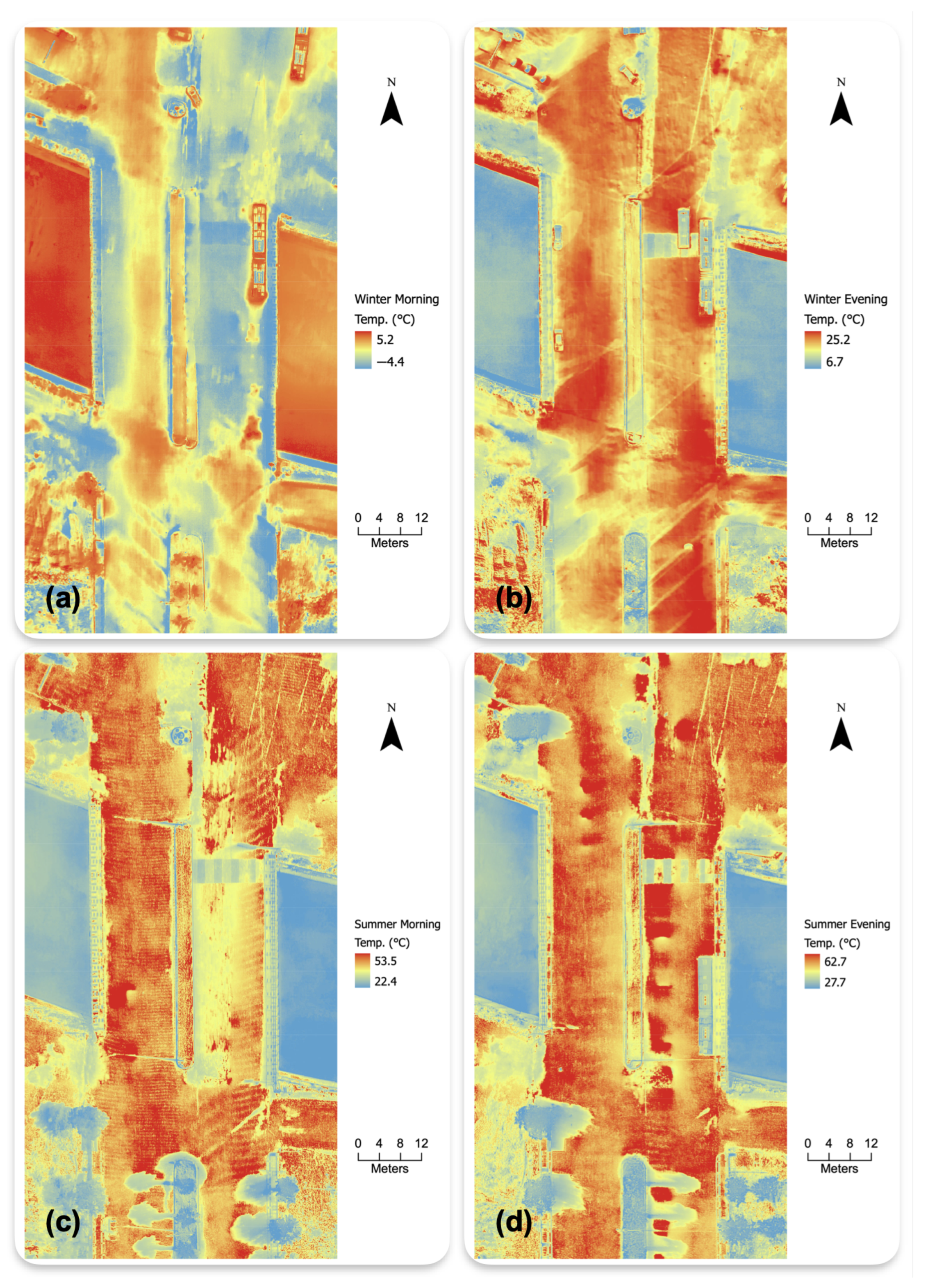
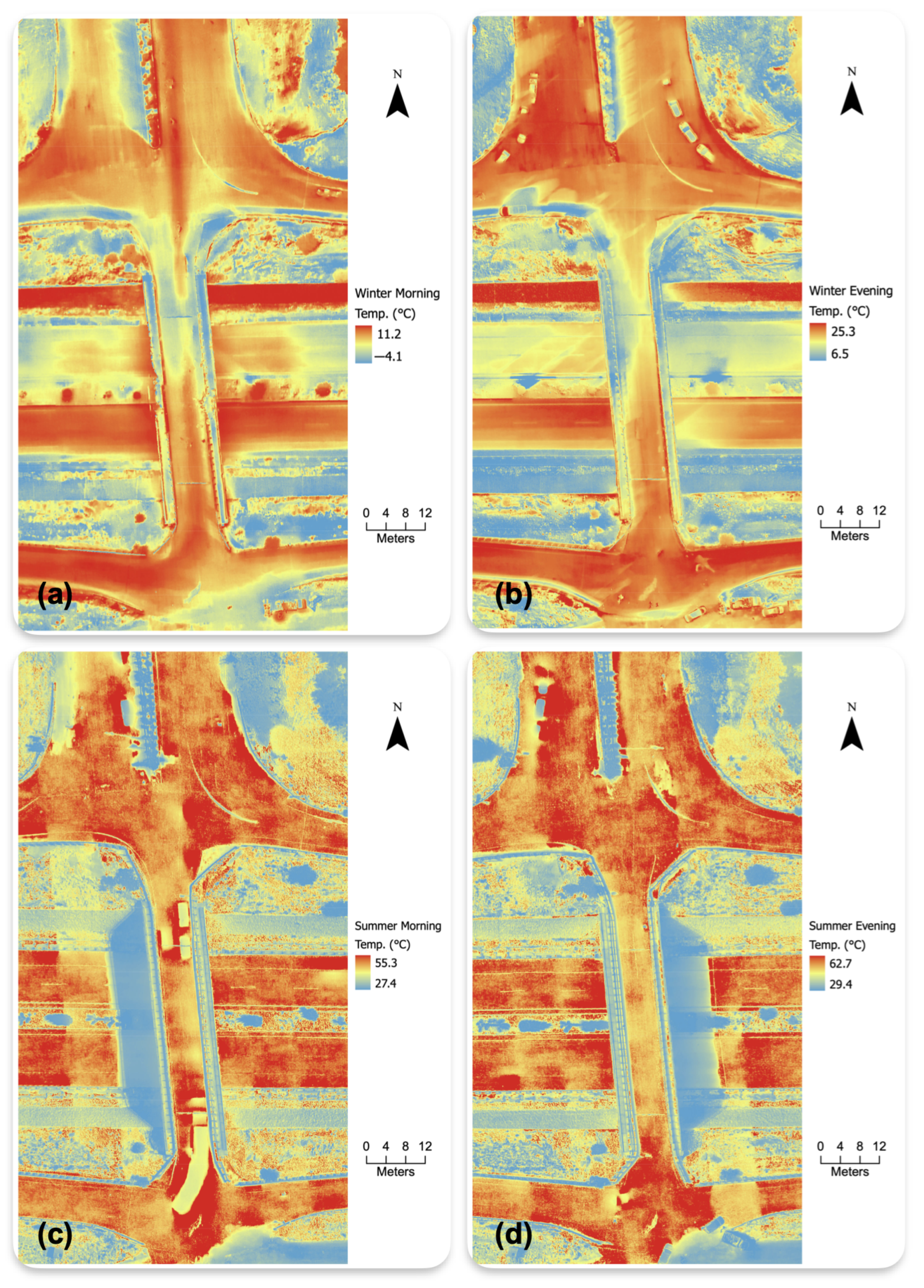
Data acquisition campaigns were conducted in two seasons, winter (January) and summer (July), to capture the extreme seasonal conditions where the most significant temperature variations occur. Spring and autumn were not included due to logistical constraints and the more gradual temperature changes in these transitional seasons, which may result in less distinct thermal contrasts. For each season, flights were performed at 08:30 and 16:30 to capture key phases of the diurnal thermal cycle. The morning (08:30) measurements represent the early warming stage following nighttime cooling, while the evening (16:30) measurements reflect the later stage of heat retention before the onset of evening cooling. A total of four flights were conducted per bridge, resulting in eight datasets for analysis.

It is important to note that our UAV thermography analysis focused exclusively on the bridge deck surfaces. We specifically targeted these areas because they are the most indicative of material-specific thermal behavior, and other structural components were not included in this study.

2.3. Data Processing

Thermal images acquired during each flight were processed using a photogrammetric workflow to generate high-resolution thermal orthophotos. The workflow included image alignment, sparse point cloud generation, dense point cloud generation, Digital Elevation Model creation, and orthophoto export. After UAV-based thermal imagery acquisition, the orthophoto generation process began with structure-from-motion (SfM) photogrammetry, a sophisticated technique that reconstructs two-dimensional thermal distributions into geometrically corrected orthomosaics [47]. SfM is particularly valuable in thermal imaging applications due to its ability to process radiometric data while preserving temperature accuracy across the merged dataset. The technique involves processing overlapping thermal images captured from multiple vantage points, employing specialized algorithms to detect and match corresponding key points across the thermal image sequence.

To capture the spatial variability in thermal behavior across the bridge, we identified three distinct zones on the bridge deck: the central zone and the entrance/exit zones. Within each zone, a stratified random sampling strategy was implemented by applying varying minimum distance criteria—ranging from $0.5$ m to 1 m—tailored to the characteristic features of that region, ensuring both randomness and a balanced spatial distribution of temperature measurement points. Specifically, 150 temperature measurements were extracted from the bridge deck, and 30 thermal reference points were systematically established in the immediate vicinity of each bridge to serve two primary functions: (1) quantifying ambient temperature conditions for environmental baseline measurements, and (2) conducting a comparative analysis of thermal characteristics between paving stone and asphalt surface materials. This $150–30$ split was chosen to enable robust statistical comparisons between different parts of each bridge as well as between each bridge and its immediate environment (Figure 2).

2.4. Analysis Methods

2.4.1. Statistical Analysis Framework

The temperature distributions of the bridge surfaces were characterized using descriptive statistics. Confidence intervals were computed at the 95% level using t-distribution methods, accounting for sample size considerations and uncertainty propagation. Comparative analysis between the bridge types was conducted using independent-samples t-tests for between-bridge comparisons and paired t-tests for within-bridge temporal analysis ($\alpha =0.05$). Effect sizes were quantified using absolute Cohen’s d, calculated as the difference between the mean values of the two compared datasets divided by the pooled standard deviation, as shown in Equation (1):

$$d={\displaystyle \frac{M_1-M_2}{{\mathrm{SD}}_{\mathrm{pooled}}}}$$

(1)

Here, $M_1$ and $M_2$ represent the mean surface temperatures of the datasets being compared, such as those of the two different bridges (water channel bridge vs. highway bridge) or the same bridge at different times of the day (morning vs. afternoon). $S{D}_{\mathrm{pooled}}$ is the pooled standard deviation, calculated as the square root of the average variance of both datasets. Established thresholds for interpretation were used: small ($0.2$), medium ($0.5$), and large ($0.8$) effects.

Figure 2. Spatial distribution of temperature measurement points across the water channel bridge (left) and highway bridge (right) captured via UAV thermal orthophoto. Blue points represent bridge surface measurements ($n=150$ per bridge) that were systematically distributed across the deck using a stratified random sampling strategy with minimum distance criteria ranging from $0.5$ m to 1 m to capture thermal variations. Yellow points indicate thermal references ($n=30$ per bridge) strategically positioned around the entrance and exit zones to establish ambient baseline conditions.

Figure 2. Spatial distribution of temperature measurement points across the water channel bridge (left) and highway bridge (right) captured via UAV thermal orthophoto. Blue points represent bridge surface measurements ($n=150$ per bridge) that were systematically distributed across the deck using a stratified random sampling strategy with minimum distance criteria ranging from $0.5$ m to 1 m to capture thermal variations. Yellow points indicate thermal references ($n=30$ per bridge) strategically positioned around the entrance and exit zones to establish ambient baseline conditions.

Building on these foundational assessments, temporal patterns were examined using a repeated-measures design for diurnal comparisons and an independent-samples approach for seasonal variations. Surface and thermal reference point temperature analysis was performed using a balanced sampling approach (150 surface measurements and 30 thermal reference points per bridge), with differences evaluated through paired t-tests. Bridge type temperature variations were assessed using independent-samples t-tests across four temporal conditions, with effect sizes quantified for practical significance. Visualization incorporated standardized box plots with $1.5\times$ IQR (interquartile range) outlier criteria, enabling direct comparison of thermal patterns between bridge types and temporal conditions.

2.4.2. Material Thermal Characterization

The material thermal behavior analysis employed a systematic protocol to characterize the thermal properties and responses of two primary surface materials: paving stone (water channel bridge) and asphalt (highway bridge). Thermal reference points ($n=30$ per bridge) were established in the immediate vicinity of each bridge structure to enable direct comparison between material types.

A correlation analysis was developed to examine the relationships between material properties and surface thermal behavior. The Pearson correlation coefficients were used to assess associations between surface temperatures and key material characteristics. These coefficients were computed across all temporal conditions (winter–summer, morning–evening) to quantify the strength and direction of material-specific thermal responses.

2.4.3. Thermal Response Metrics

The thermal behavior of bridge structures was characterized through several quantitative metrics designed to capture different aspects of thermal response patterns. The primary analysis focused on heating rates calculated from temperature measurements taken at standardized morning (08:30) and evening (16:30) times, which ensured a consistent 8 h measurement interval. The heating rate (R) was computed as the ratio of temperature change ($\Delta T$) to the time interval ($\Delta t$), providing a standardized measure of thermal response speed across different bridge types and seasonal conditions. These thermal response metrics were selected to systematically assess how bridge surfaces absorb and dissipate heat under different environmental conditions. Heating rate provides insight into the rate of thermal energy accumulation, temperature differentials quantify the influence of surrounding environmental factors, and statistical comparisons help evaluate material-dependent thermal stability.

2.4.4. Environmental Response Analysis

Surface ambient temperature differential analysis was performed through a systematic protocol to evaluate how bridges respond to changing environmental conditions. Environmental baseline conditions were established using a temperature sensor positioned adjacent to each bridge structure (<10 m distance) to record ambient temperature measurements concurrent with the UAV thermal imaging operations. Correlation analysis between surface and ambient temperatures was performed using Pearson’s correlation coefficients, with statistical significance assessed at $\alpha =0.05$. Temperature differentials ($\Delta T$) were calculated by subtracting ambient temperatures from the mean surface temperatures derived from the systematically distributed measurement points ($n=150$ per bridge), with positive values indicating surface temperatures exceeding ambient conditions. Standard error estimates for temperature differentials were computed using propagation of uncertainty principles, incorporating both instrument measurement uncertainty ($\pm 0.5$ °C) and spatial variation across the sampling points. The temporal stability of environmental coupling was evaluated through analysis of surface ambient temperature relationships across four discrete measurement periods (winter morning/evening, summer morning/evening), with coefficients of determination ($R^2$) being calculated to quantify the strength of environmental coupling.

3. Results

3.1. Thermal Distribution Characteristics

To comprehensively analyze thermal dynamics in the study, thermal orthophotos were generated to include both the bridges and their surrounding environments. Rather than isolating the bridges, this approach captures thermal variations in a broader context, incorporating all surrounding surfaces from multiple directions. By doing so, the assessment provides a more accurate representation of the thermal interactions between the bridges and their environments.

The generated thermal orthophotos for the water channel bridge captured both the bridge structure and its surrounding environment, ensuring a comprehensive assessment of the thermal dynamics (Figure 3). Temperature fluctuations ranged from $-4.4$ °C to $5.2$ °C during winter mornings, with pronounced thermal stratification near the water interface. Evening measurements indicated significant thermal increases, reaching $6.7$–$25.2$ °C. Under summer conditions, thermal responses were more pronounced, with morning temperature variations from $22.4$ to $53.5$ °C and evening temperatures reaching a maximum of $62.7$ °C. These values represent not only the bridge surface but also adjacent areas, reflecting the broader thermal interactions within the study environment.

The generated thermal orthophotos for the highway bridge encompassed both the bridge structure and its surrounding environment to provide a comprehensive analysis of thermal dynamics. Winter morning temperatures ranged from $-4.1$ °C to $11.2$ °C, reflecting variations across the bridge and adjacent surfaces. Summer measurements revealed intense heating patterns, with morning temperatures varying from $27.4$ °C to $55.3$ °C and evening peaks reaching $62.7$ °C (Figure 4). The thermal orthophotos encompassed both the bridge structure and its adjacent environmental context, providing comprehensive spatial temperature distributions.

3.2. Statistical Characterization of Surface Temperatures

3.2.1. Descriptive Statistics

To quantify surface temperature variations across different seasonal and diurnal conditions, 150 thermal measurements were collected from both bridge surfaces, and the results are summarized in

Table 1. Descriptive statistics of bridge surface temperatures by bridge type and temporal condition.

Bridge Type	Condition	n	Min (°C)	Max (°C)	Mean (°C)	Med. (°C)	SD (°C)	SE (°C)	95% CI
Water Channel	Winter Morning	150	$-3.95$	$2.83$	$0.02$	$0.42$	$1.54$	$0.13$	$[-0.23,0.26]$
	Winter Evening	150	$14.89$	$24.95$	$21.82$	$21.97$	$2.34$	$0.19$	$[21.45,22.20]$
	Summer Morning	150	$33.42$	$53.46$	$48.40$	$49.02$	$3.43$	$0.28$	$[47.85,48.95]$
	Summer Evening	150	$47.39$	$62.69$	$55.43$	$54.88$	$3.48$	$0.28$	$[54.88,55.99]$
Highway	Winter Morning	150	$-1.60$	$9.75$	$5.21$	$6.32$	$3.27$	$0.27$	$[4.69,5.74]$
	Winter Evening	150	$7.58$	$23.02$	$17.31$	$18.26$	$3.98$	$0.32$	$[16.67,17.94]$
	Summer Morning	150	$34.34$	$55.30$	$47.72$	$47.05$	$5.46$	$0.45$	$[46.85,48.59]$
	Summer Evening	150	$31.60$	$61.56$	$49.43$	$50.26$	$5.66$	$0.46$	$[48.52,50.33]$

Note: n = sample size; SD = standard deviation; SE = standard error; CI = confidence interval. All temperature measurements are in degrees Celsius (°C). Confidence intervals are calculated at the 95% level.

. Key descriptive statistics, including minimum and maximum values, mean temperatures, standard deviations, and confidence intervals, were computed to assess thermal variability.

The water channel bridge exhibited moderate temperature variations, with standard deviations ranging from $1.54$ °C (winter morning) to $3.48$ °C (summer evening), whereas the highway bridge demonstrated greater thermal variability, with standard deviations from $3.27$ °C to $5.66$ °C. The most pronounced temperature range was observed in the highway bridge during summer evenings, spanning $29.96$ °C (from $31.60$ °C to $61.56$ °C), while the water channel bridge exhibited more constrained thermal behavior, particularly during winter mornings, with a range of $6.78$ °C (from $-3.95$ °C to $2.83$ °C). Measurement precision remained high across all conditions, with 95% confidence intervals consistently spanning less than 2 °C, except for under highway bridge summer conditions, where increased thermal variability was observed. Standard deviations and temperature ranges were consistently lower for the water channel bridge, indicating reduced thermal variability compared to the highway bridge.

3.2.2. Temperature Distribution Analysis

As illustrated in Figure 5, the box plot visualization provides a detailed representation of temperature distributions across seasonal and diurnal cycles. The plot reveals distinct thermal regimes between the two bridge types, with the highway bridge exhibiting wider interquartile ranges, particularly during winter morning conditions where temperatures ranged from $-1.6$ °C to $9.7$ °C. In contrast, the water channel bridge displays more compressed temperature distributions, especially evident in the winter morning measurements. The visualization also captures the temporal evolution of surface temperatures, with the highway bridge showing more pronounced temperature variations in summer evening conditions, ranging from $31.6$ °C to $61.6$ °C with several outliers.

3.3. Comparative Thermal Analysis

3.3.1. Surface and Thermal Reference Point Temperature Analysis

Thermal behavior analysis was conducted using a balanced sampling approach incorporating 150 surface temperature measurements and 30 thermal reference point measurements for each bridge type. Statistical significance was assessed using paired t-tests, with effect sizes quantified through Cohen’s d. To evaluate the precision of the temperature measurements, 95% confidence intervals were calculated (

Table 2. Comparative analysis of bridge surface and thermal reference point temperatures.

Bridge Type	Condition	Surface Temp. (°C)	Thermal Ref. Temp. (°C)	Diff. (°C)	t-Stat.	Effect Size (d)	Sig.
Water Channel	Winter Morning	$0.02\pm 1.54$	$1.24\pm 2.09$	$-1.22$	$-3.039$	$0.75$	**
	Winter Evening	$21.82\pm 2.34$	$21.12\pm 2.58$	$0.70$	$1.383$	$0.30$	ns
	Summer Morning	$48.40\pm 3.43$	$47.48\pm 3.63$	$0.92$	$1.284$	$0.27$	ns
	Summer Evening	$55.43\pm 3.48$	$56.61\pm 4.39$	$-1.18$	$-1.384$	$0.32$	ns
Highway	Winter Morning	$5.21\pm 3.27$	$7.04\pm 2.08$	$-1.83$	$-3.943$	$0.59$	***
	Winter Evening	$17.31\pm 3.98$	$21.99\pm 2.03$	$-4.68$	$-9.505$	$1.26$	***
	Summer Morning	$47.72\pm 5.46$	$50.21\pm 4.72$	$-2.49$	$-2.568$	$0.47$	*
	Summer Evening	$49.43\pm 5.66$	$57.50\pm 5.52$	$-8.08$	$-7.288$	$1.43$	***

Note: Values are presented as mean ± standard deviation. Sample sizes: surface temperatures $n=150$, thermal reference points $n=30$. Effect size reported as absolute Cohen’s d. Significance levels: * $p<0.05$, ** $p<0.01$, *** $p<0.001$, ns = not significant.

).

The water channel bridge exhibited selective temporal sensitivity to thermal differentials, with statistically significant differences primarily observed during winter conditions. The most pronounced differential occurred on winter mornings, where surface temperatures were, on average, $-1.22$ °C lower than the thermal reference points ($p<0.01$), demonstrating medium-to-large practical significance (Cohen’s $d=0.75$). In contrast, summer measurements indicated more moderate thermal behavior. Morning temperatures exhibited a non-significant positive differential of $0.92$ °C ($d=0.27$), while evening measurements showed a non-significant negative differential of $-1.18$ °C ($d=0.32$).

Figure 5. Box plot distribution of surface temperatures across seasonal and diurnal cycles for highway and water channel bridges.

Figure 5. Box plot distribution of surface temperatures across seasonal and diurnal cycles for highway and water channel bridges.

The highway bridge exhibited consistent and highly significant thermal differentials across multiple temporal conditions throughout the study period. The most pronounced temperature difference occurred during summer evenings, with surface temperatures averaging $8.08$ °C below the thermal reference points ($p<0.001$), indicating very large practical significance. This thermal differential pattern persisted across other conditions, with winter evenings showing a $-4.68$ °C differential, winter mornings a $-1.83$ °C differential, and summer mornings a $-2.49$ °C differential. Temporal analysis identified consistent patterns of significant temperature differentials across all conditions, with particularly pronounced effects during evening periods.

3.3.2. Comparative Analysis of Bridge Temperature Variations

Independent-samples t-tests were performed to assess temperature differences between water channel and highway bridges across four temporal conditions. Each analysis included 150 measurements per condition for each bridge type. Three of the four comparisons yielded statistically significant differences ($p<0.001$) with substantial effect sizes (

Table 3. Statistical comparison of bridge temperature variations.

Condition	Water Channel (°C)	Highway (°C)	Difference	t-Statistic	df	Effect Size (d)	Sig.
Winter Morning	$0.02\pm 1.54$	$5.21\pm 3.27$	$-5.20$	$-17.62$	298	$2.03$	***
Winter Evening	$21.82\pm 2.34$	$17.31\pm 3.98$	$4.52$	$11.99$	298	$1.38$	***
Summer Morning	$48.40\pm 3.43$	$47.72\pm 5.46$	$0.68$	$1.29$	298	$0.15$	ns
Summer Evening	$55.43\pm 3.48$	$49.43\pm 5.66$	$6.01$	$11.07$	298	$1.28$	***

Note: Values are presented as mean ± standard deviation. Effect size is reported as absolute Cohen’s d. Significance levels: *** $p<0.001$, ns = not significant. Sample size: $n=150$ for each bridge type and condition, df: degrees of freedom.

).

During winter mornings, the highway bridge exhibited significantly higher temperatures than the water channel bridge with the largest effect size ($d=2.03$). In contrast, winter evening measurements showed higher temperatures in the water channel bridge relative to the highway bridge ($d=1.38$).

The most pronounced temperature differential occurred during winter mornings, with the highway bridge maintaining significantly higher temperatures ($-5.20$ °C higher) compared to the water channel bridge, exhibiting the largest effect size ($d=2.03$). In contrast, summer morning measurements showed minimal thermal differentiation between the bridge types, with only a $0.68$ °C difference that was not statistically significant ($d=0.15$).

Pattern analysis showed distinct variations in thermal behavior between the two bridge types. Temperature differentials ranged from $0.68$ °C in summer mornings to $6.01$ °C during summer evenings. Effect size calculations revealed substantial magnitudes in three temporal conditions, particularly during winter mornings and evenings. The water channel bridge exhibited more stable thermal characteristics, as reflected in the lower standard deviations in temperature measurements compared to the highway bridge. Notably, the water channel bridge maintained higher average temperatures in most conditions, except during winter mornings.

3.4. Material Thermal Behavior

3.4.1. Material-Specific Thermal Response Analysis

The comparative analysis of thermal reference point temperatures ($n=30$ per bridge) between paving stone (water channel) and asphalt (highway) surfaces revealed temporal patterns in the thermal behavior. Statistical assessment using independent-samples t-tests, along with effect size calculations, identified significant material-dependent variations across different temporal conditions (

Table 4. Statistical comparison of thermal reference point temperatures by material type and temporal condition.

Temporal Condition	Material Type	Mean Temp (°C)	SD (°C)	Diff. (°C)	t-Stat.	Effect Size (d)	Sig.
Winter Morning	Paving Stone (Water Channel)	$1.24$	$2.09$	$-5.80$	$-10.769$	$2.78$	***
	Asphalt (Highway)	$7.04$	$2.08$
Winter Evening	Paving Stone (Water Channel)	$21.12$	$2.58$	$-0.87$	$-1.452$	$0.38$	ns
	Asphalt (Highway)	$21.99$	$2.03$
Summer Morning	Paving Stone (Water Channel)	$47.48$	$3.63$	$-2.73$	$-5.869$	$0.87$	*
	Asphalt (Highway)	$50.21$	$4.72$
Summer Evening	Paving Stone (Water Channel)	$56.61$	$4.39$	$-0.90$	$-1.554$	$0.18$	ns
	Asphalt (Highway)	$57.50$	$5.52$

$n=30$ thermal reference points per bridge type. Significance levels: * $p<0.05$, *** $p<0.001$, ns = not significant. Effect size reported as absolute Cohen’s d.

).

The paving stone surface of the water channel bridge exhibited seasonal thermal variation, with mean temperatures ranging from $1.24$ °C to $56.61$ °C across temporal conditions. The asphalt surface of the highway bridge displayed a similar thermal profile, with temperatures varying between $7.04$ °C and $57.50$ °C. Standard deviations in temperature measurements showed variable patterns; while similar on winter mornings, paving stone demonstrated lower thermal variability during summer conditions, particularly in the morning ($SD=3.63$ °C vs. $4.72$ °C) and evening ($SD=4.39$ °C vs. $5.52$ °C).

During winter mornings, asphalt surfaces exhibited substantially higher temperatures than paving stone, with a significant differential of $-5.80$ °C ($p<0.001$) and a notably large effect size ($d=2.78$). Evening measurements during winter showed a non-significant temperature difference, with asphalt maintaining marginally higher temperatures than paving stone. The observed thermal behavior pattern reflects the distinct absorption and retention characteristics of the two materials during cold weather conditions.

Summer conditions continued to evoke material-dependent thermal responses, though with characteristics distinct from winter patterns. Morning measurements showed asphalt temperatures significantly exceeding those of paving stone by $2.73$ °C ($p<0.05$) with a large effect size ($d=0.87$). Evening measurements displayed minimal thermal differentiation between the two surface types, with a non-significant difference. The observed temporal patterns of thermal differentials suggest complex heat transfer mechanisms specific to each material type.

Morning measurements consistently revealed statistically significant temperature differentials, while evening conditions showed convergence in the thermal behavior of the materials. The greatest differentiation occurred on winter mornings ($-5.80$ °C), with the thermal gap narrowing considerably during evening periods in both seasons. Effect sizes demonstrated a notable pattern, ranging from very large during winter mornings ($d=2.78$) to small during summer evenings ($d=0.18$), with an intermediate peak during summer mornings ($d=0.87$).

The results indicate consistent material-dependent thermal behavior patterns, with thermal differentials varying across temporal conditions. Pronounced morning differentials and evening convergence patterns were observed, reflecting variations in thermal inertia between paving stone and asphalt surfaces. The data demonstrate that asphalt surfaces maintain significantly higher temperatures during morning periods, particularly in winter, whereas evening measurements show thermal convergence between the materials. Effect size calculations confirmed substantial differences in thermal behavior between the two materials during morning periods, with winter mornings exhibiting the most pronounced effect ($d=2.78$), highlighting distinct temporal patterns in thermal retention and dissipation characteristics.

3.4.2. Material–Temperature Correlations

Pearson correlation coefficients were calculated to assess the thermal response characteristics of the paving stone and asphalt surfaces across four temporal conditions (

Table 5. Pearson correlation coefficients between material type and surface temperatures.

Temporal Condition	Correlation Coefficient (r)	p-Value	Statistical Significance
Winter Morning	$0.714$	<$0.001$	***
Winter Evening	$-0.571$	<$0.001$	***
Summer Morning	$-0.075$	$0.197$	ns
Summer Evening	$-0.540$	<$0.001$	***

Note: Significance levels: *** $p<0.001$, ns = not significant.

). The analysis revealed strong positive correlations during winter mornings and moderate negative correlations during winter evenings, with correlation coefficients of $0.714$ and $-0.571$, respectively.

Summer conditions exhibited more variable correlations, with morning measurements showing a weak, non-significant correlation and evening measurements displaying a moderate negative correlation.

Winter conditions produced the most pronounced material-dependent thermal responses, with substantial effect sizes observed in both the morning and evening measurements. The temporal analysis revealed complex patterns between material properties and environmental conditions, particularly in the differential heating and cooling responses during diurnal cycles. While summer evening measurements showed significant material-specific patterns, summer morning measurements exhibited weak, non-significant correlations, suggesting that the thermal behavior differences between the two surface types are most pronounced during specific temporal conditions.

3.4.3. Thermal Response Characteristics

Thermal behavior analysis was conducted through systematic measurements at 08:30 and 16:30 local time, establishing an 8-h measurement interval for calculating heating rates.

Table 6. Heating rate analysis by bridge type and season.

Bridge Type	Season	Mean $\mathbf{\Delta }\mathit{T}$ (°C)	Heating Rate (°C/h)
Water Channel	Winter	$+21.80$	$2.73\pm 0.22$
	Summer	$+7.03$	$0.88\pm 0.31$
Highway	Winter	$+12.10$	$1.51\pm 0.33$
	Summer	$+1.71$	$0.21\pm 0.49$

Note: Values are presented as mean ± standard deviation. Heating rates were calculated over exact 8 h periods (08:30–16:30).

presents a comprehensive analysis of the heating rates across bridge types and seasonal conditions. The results indicate distinct thermal response patterns, with the water channel bridge exhibiting significantly higher heating rates in winter ($2.73$ °C/h) compared to the highway bridge ($1.51$ °C/h, $p<0.001$). This differential was less pronounced under summer conditions, with the water channel bridge maintaining a substantially higher heating rate of $0.88$ °C/h than the highway bridge’s $0.21$ °C/h ($p<0.05$). The seasonal heating rate differentials indicated greater temporal variation in the water channel bridge compared to the highway bridge, reflecting distinct thermal response characteristics between the structures.

3.5. Environmental Response Analysis

Environmental monitoring during the measurement campaigns identified substantial temporal variations in the ambient conditions across seasonal and diurnal cycles. Winter measurements were conducted at ambient temperatures of $7.00$ °C (morning) and $10.80$ °C (evening), while summer measurements occurred under warmer conditions of $32.70$ °C (morning) and $41.50$ °C (evening). Under these varying environmental conditions, statistical analysis of temperature differentials (

Table 7. Temporal analysis of bridge surface ambient temperature differentials.

Temporal Condition	Water Channel Bridge $\mathbf{\Delta }\mathit{T}$ (°C)	Highway Bridge ΔT (°C)
Winter Morning	$-6.98$	$-1.79$
Winter Evening	$+11.02$	$+6.51$
Summer Morning	$+15.70$	$+15.02$
Summer Evening	$+13.93$	$+7.93$

Note: $\Delta T$ represents the difference between surface and ambient temperatures (surface temperature minus ambient temperature).

) identified characteristic thermal signatures for each bridge type. The water channel bridge exhibited more pronounced temperature differentials during most temporal conditions, with values ranging from $-6.98$ °C on winter mornings to $+15.70$ °C on summer mornings. The highway bridge generally showed more moderate differentials, particularly in winter conditions ($-1.79$ °C to $+6.51$ °C), though it demonstrated comparable thermal deviation during summer mornings ($+15.02$ °C).

Correlation analysis revealed distinct thermal behavior patterns for the two bridge types (

Table 8. Correlation analysis of ambient and bridge surface temperatures.

Metric	Water Channel Bridge	Highway Bridge
Pearson’s Correlation (r)	$0.961$	$0.975$
Coefficient of Determination ($R^2$)	$0.924$	$0.951$
Mean Temperature Differential ($\Delta T$)	8.42 °C	6.92 °C
Standard Error of Estimate	5.86 °C	4.73 °C

Note: Temperature differentials were calculated as the absolute differences between surface (mean of surface measurement points) and ambient temperatures ($n=4$ temporal conditions).

). The analysis was conducted using mean values derived from the bridge surface measurement points. Both bridges demonstrated strong correlations with ambient temperatures, with the highway bridge exhibiting a marginally higher correlation ($r=0.975$) compared to the water channel bridge ($r=0.961$), suggesting slightly more predictable thermal response patterns.

Temporal analysis revealed the greatest thermal deviation under summer morning conditions for both structures, with the water channel bridge exhibiting a greater departure from the ambient temperatures than the highway bridge. The highway bridge maintained relatively consistent thermal differentials across seasonal conditions, particularly in winter, where its minimum differential indicated a moderate departure from ambient conditions relative to the water channel bridge. The results suggest that water body proximity may amplify thermal response variations, particularly during extreme temperature conditions.

The results indicate differential thermal responses between the bridges, with the water channel bridge exhibiting greater thermal independence from ambient conditions. These variations highlight the influence of environmental context on bridge thermal behavior.

4. Discussion

This study reveals fundamental differences in thermal behavior between water channel and highway bridges through UAV-based thermography, thereby demonstrating the viability of aerial thermography with high-precision sensors for detailed bridge thermal analysis. The systematic sampling approach—incorporating 150 surface measurements and 30 thermal reference points per bridge—provides an effective framework for comparative thermal assessment. The high measurement precision, evidenced by the narrow confidence intervals in winter conditions, validates the reliability of this methodology for structural thermal evaluation. Furthermore, the study establishes a comprehensive statistical framework for analyzing structural thermal behavior encompassing temporal analysis across diurnal and seasonal cycles, material-specific thermal response characterization, and the assessment of environmental coupling.

The observed thermal behavior patterns indicate a complex interplay between environmental context and structural characteristics. Specifically, the presence of water appears to create a microclimate that moderates temperature fluctuations, acting as a thermal buffer. This buffering effect is particularly evident in the consistently lower standard deviations of temperature measurements for the water channel bridge, suggesting that water bodies may form thermal boundary layers that influence structural temperature dynamics. The mechanism likely involves both convective heat transfer through air movement and radiative heat exchange with the water surface, thereby creating a more stable thermal environment. In contrast, the highway bridge showed significant thermal differentials compared to the thermal reference points, which can be interpreted as evidence of a cooling effect facilitated by the air circulation under the bridge.

The analysis demonstrates a sophisticated interaction between material properties and environmental context that extends beyond simple thermal conductivity considerations. The distinct thermal signatures, with paving stone surfaces displaying more consistent thermal behavior than asphalt, particularly under extreme temperature conditions, highlight the impact of material choice on bridge thermal performance. This adaptive behavior suggests a dynamic thermal response system where material properties and environmental conditions create unique thermal signatures. Furthermore, material properties such as heat absorption, release capacity, and sensitivity to temperature changes contribute to thermal variations.

The superior thermal stability of paving stone surfaces suggests potential benefits for structural longevity, while the proximity of water emerges as a significant factor in thermal stabilization. Notably, evening periods exhibited more consistent thermal distributions, implying that these times may be optimal for inspection activities. The increased measurement uncertainty in summer conditions highlights the need for season-specific monitoring strategies.

Several limitations of the current study warrant consideration. First, using discrete measurement times (08:30 and 16:30) may overlook critical thermal transitions—particularly midday peak thermal conditions when solar radiation reaches maximum intensity—which suggests valuable opportunities for future research to capture more comprehensive diurnal thermal profiles. While the study primarily focused on temperature, other atmospheric factors—including humidity, wind, and ambient temperature fluctuations—could also influence thermal readings and therefore merit further investigation. The seasonal dichotomy approach (winter/summer) effectively captured extreme thermal conditions but excluded transitional seasons that might reveal distinct thermal adaptation patterns. Though this selection was based on logistical considerations and the need to observe maximum thermal contrast, expanding temporal coverage to include spring and autumn would provide a more nuanced understanding of seasonal thermal transitions.

Moreover, the accuracy of UAV thermal measurements is closely tied to sensor calibration; even minor deviations can introduce significant uncertainties. Although direct absolute temperatures were not required in this study due to the focus on comparative analysis, variations in atmospheric conditions could still have influenced thermal readings. To facilitate reliable comparisons, it is essential to minimize environmental variability by collecting data within short temporal intervals and ensuring consistent flight parameters. Nonetheless, maintaining uniform flight conditions—such as altitude, image overlap, and sensor orientation—across diverse environmental settings remains a substantial operational challenge that may compromise data uniformity. Finally, it is important to note that the inability to completely isolate material effects from environmental influences stems from the fact that the two bridges differ not only in surface materials—paving stone versus asphalt—but also in their surrounding conditions. While the two selected bridge types represent common infrastructure configurations, expanding the bridge typology to include varying structural designs, span lengths, orientation angles, and construction materials would enhance the generalizability of findings. Regions with spatially proximate yet structurally diverse bridge types under similar environmental conditions would enable broader validation of thermal behavior patterns and facilitate simultaneous data collection for improved comparative analysis.

The findings have practical implications for bridge health monitoring and maintenance. UAV-based thermal surveys can help detect material degradation by identifying abnormal temperature patterns, aiding in early maintenance planning. Additionally, insights into material-specific thermal behavior can optimize maintenance schedules and inform bridge design improvements, particularly in environments affected by temperature fluctuations and water proximity.

5. Conclusions and Recommendations

This study examined the seasonal and diurnal thermal dynamics of bridge infrastructure using high-resolution UAV thermography, comparing a water channel bridge and a highway bridge. The research systematically addressed four fundamental questions related to bridge thermal behavior, environmental influences, material responses, and analytical approaches.

Regarding spatial temperature distributions [RQ1], the analysis revealed distinct differences in thermal behavior between the bridge types, with the water channel bridge exhibiting significantly more stable thermal characteristics than the highway bridge. The investigation of environmental factor relationships [RQ2] uncovered complex patterns of environmental coupling between the bridge structures and their surroundings. Analysis of material-specific thermal responses [RQ3] identified distinct thermal signatures for the paving stone and asphalt surfaces. The implementation of the statistical framework [RQ4] successfully quantified thermal variations and confirmed the effectiveness of UAV thermography for thermal assessment. The findings provide a comprehensive foundation for understanding the complex thermal interactions between structural materials and environmental factors, paving the way for further advancements in bridge thermal assessment and monitoring strategies.

Future research should focus on continuous monitoring systems, responses to extreme weather conditions, and detailed models for water-proximity effects. These investigations should emphasize location-specific approaches to infrastructure design and monitoring, particularly considering the implications for urban infrastructure planning in regions experiencing increasing temperature extremes. Additionally, regions with spatially close yet diverse bridge types under similar environmental conditions would enable broader validation of thermal behavior patterns and facilitate simultaneous data collection for improved generalizability.

References

1. Hartmann, J. Bolstering the safety of America’s bridges for half a century. Public Roads 2021, 85, 23–26. [Google Scholar]
2. Borah, S.; Al-Habaibeh, A.; Kromanis, R. The Effect of Temperature Variation on Bridges—A Literature Review. In Energy and Sustainable Futures; Springer Proceedings in Energy; Springer: Cham, Switzerland, 2021. [Google Scholar]
3. Burdet, O. Thermal effects in the long-term monitoring of bridges. In Proceedings of the 34th International Symposium on Bridge and Structural Engineering, Venice, Italy, 22–24 September 2010; pp. 1–8. [Google Scholar]
4. Nasr, A.; Kjellström, E.; Björnsson, I.; Honfi, D.; Ivanov, O.L.; Johansson, J. Bridges in a changing climate: A study of the potential impacts of climate change on bridges and their possible adaptations. Struct. Infrastruct. Eng. 2019, 16, 738–749. [Google Scholar] [CrossRef]
5. Han, Q.; Ma, Q.; Xu, J.; Liu, M. Structural health monitoring research under varying temperature condition: A review. J. Civ. Struct. Health Monit. 2021, 11, 149–173. [Google Scholar] [CrossRef]
6. Imbsen, R.A.; Vandershaf, D.E. Thermal effects in concrete bridge superstructures. Transp. Res. Rec. 1984, 950, 101–113. [Google Scholar]
7. Lorenz, R.; Petryna, Y.; Lubitz, C.; Lang, O.; Wegener, V. Thermal deformation monitoring of a highway bridge: Combined analysis of geodetic and satellite-based InSAR measurements with structural simulations. J. Civ. Struct. Health Monit. 2024, 14, 1237–1255. [Google Scholar] [CrossRef]
8. Xia, Y.; Zhou, Y. Temperature Behavior of Bridges, 1st ed.; CRC Press: Boca Raton, FL, USA, 2025. [Google Scholar] [CrossRef]
9. Zuk, W. Thermal behavior of composite bridges—Insulated and uninsulated. Highw. Res. Rec. 1965, 76, 150–173. [Google Scholar]
10. Wah, T.; Kirksey, R.E. Thermal characteristics of highway bridges. Highw. Res. Board Nchrp Summ. 1969, 79–95. [Google Scholar]
11. Fu, H.C.; Ng, S.F.; Cheung, M.S. Thermal behavior of composite bridges. J. Struct. Eng. 1990, 116, 330–347. [Google Scholar] [CrossRef]
12. Chang, S.P.; Im, C.K. Thermal behaviour of composite box-girder bridges. Proc. Inst. Civ. Eng.-Struct. Build. 2000, 140, 247–256. [Google Scholar] [CrossRef]
13. Liu, W.; Zhou, E.; Wang, Y.; Meggers, D.A.; Plunkett, J. Long-Term Remote Monitoring of Thermal Response of No-Name Creek FRP Bridge to Climate; Technical Report K-TRAN: KU-08-6; Kansas State University Transportation Center: Manhattan, KS, USA, 2008. [Google Scholar]
14. Yang, D.H.; Yi, T.H.; Li, H.N.; Zhang, Y.F. Monitoring and analysis of thermal effect on tower displacement in cable-stayed bridge. Measurement 2018, 115, 249–267. [Google Scholar] [CrossRef]
15. Kromanis, R.; Kripakaran, P. Predicting thermal response of bridges using regression models derived from measurement histories. Comput. Struct. 2014, 136, 64–77. [Google Scholar] [CrossRef]
16. Escobar-Wolf, R.; Oommen, T.; Brooks, C.N.; Dobson, R.J.; Ahlborn, T.M. Unmanned aerial vehicle (UAV)-based assessment of concrete bridge deck delamination using thermal and visible camera sensors: A preliminary analysis. Res. Nondestruct. Eval. 2018, 29, 183–199. [Google Scholar] [CrossRef]
17. Li, L.; Chen, B.; Zhou, L.; Xia, Q.; Zhou, Y.; Zhou, X.; Xia, Y. Thermal behaviors of bridges—A literature review. Adv. Struct. Eng. 2023, 26, 1423–1441. [Google Scholar] [CrossRef]
18. Kara, N.; Şişman, H.A.; Özcan, O.; Özcan, O.; Erten, E. InSAR coupled with UAV-based infrared thermography in the context of bridge monitoring. In Proceedings of the 2023 IEEE International Geoscience and Remote Sensing Symposium (IGARSS), Pasadena, CA, USA, 16–21 July 2023; pp. 123–126. [Google Scholar]
19. Abdel-Maksoud, H. Combining UAV-LiDAR and UAV-Photogrammetry for bridge assessment and infrastructure monitoring. Arab. J. Geosci. 2024, 17, 144. [Google Scholar] [CrossRef]
20. Zhang, Q.; Ro, S.H.; Wan, Z.; Babanajad, S.; Braley, J.; Barri, K.; Alavi, A.H. Automated unmanned aerial vehicle-based bridge deck delamination detection and quantification. Transp. Res. Rec. 2023, 2677, 24–36. [Google Scholar] [CrossRef]
21. Santesteban, L.G.; Di Gennaro, S.F.; Herrero-Langreo, A.; Miranda, C.; Royo, J.B.; Matese, A. High-resolution UAV-based thermal imaging to estimate the instantaneous and seasonal variability of plant water status within a vineyard. Agric. Water Manag. 2017, 183, 49–59. [Google Scholar] [CrossRef]
22. Ortiz-Sanz, J.; Gil-Docampo, M.; Arza-García, M.; Cañas-Guerrero, I. IR thermography from UAVs to monitor thermal anomalies in the envelopes of traditional wine cellars: Field test. Remote Sens. 2019, 11, 1424. [Google Scholar] [CrossRef]
23. Perich, G.; Hund, A.; Anderegg, J.; Roth, L.; Boer, M.P.; Walter, A.; Liebisch, F.; Aasen, H. Assessment of multi-image unmanned aerial vehicle based high-throughput field phenotyping of canopy temperature. Front. Plant Sci. 2020, 11, 150. [Google Scholar] [CrossRef]
24. Nieto, H.; Kustas, W.P.; Torres-Rúa, A.; Alfieri, J.G.; Gao, F.; Anderson, M.C.; White, W.A.; Song, L.; Alsina, M.D.M.; Prueger, J.H.; et al. Evaluation of TSEB turbulent fluxes using different methods for the retrieval of soil and canopy component temperatures from UAV thermal and multispectral imagery. Irrig. Sci. 2019, 37, 389–406. [Google Scholar] [CrossRef]
25. Casana, J.; Wiewel, A.; Cool, A.; Hill, C.; Fisher, K.D.; Laugier, E.J. Archaeological aerial thermography in theory and practice. Adv. Archaeol. Pract. 2017, 5, 310–327. [Google Scholar] [CrossRef]
26. Zheng, H.; Zhong, X.; Yan, J.; Zhao, L.; Wang, X. A thermal performance detection method for building envelope based on 3D model generated by UAV thermal imagery. Energies 2020, 13, 6677. [Google Scholar] [CrossRef]
27. Feng, Y.; Du, S.; Myint, S.W.; Shu, M. Do urban functional zones affect land surface temperature differently? A case study of Beijing, China. Remote Sens. 2019, 11, 1802. [Google Scholar] [CrossRef]
28. Chudnovsky, A.; Ben-Dor, E.; Saaroni, H. Diurnal thermal behavior of selected urban objects using remote sensing measurements. Energy Build. 2004, 36, 1063–1074. [Google Scholar] [CrossRef]
29. Yin, C.; Yuan, M.; Lu, Y.; Huang, Y.; Liu, Y. Effects of urban form on the urban heat island effect based on spatial regression model. Sci. Total Environ. 2018, 634, 696–704. [Google Scholar] [CrossRef] [PubMed]
30. Xu, S.; Yang, K.; Xu, Y.; Zhu, Y.; Luo, Y.; Shang, C.; Zhang, J.; Zhang, Y.; Gao, M.; Wu, C. Urban land surface temperature monitoring and surface thermal runoff pollution evaluation using UAV thermal remote sensing technology. Sustainability 2021, 13, 11203. [Google Scholar] [CrossRef]
31. Naughton, J.; McDonald, W. Evaluating the variability of urban land surface temperatures using drone observations. Remote Sens. 2019, 11, 1722. [Google Scholar] [CrossRef]
32. Soto-Estrada, E.; Correa-Echeverri, S.; Posada-Posada, M.I. Thermal analysis of urban environments in Medellin, Colombia, using an unmanned aerial vehicle (UAV). J. Urban Environ. Eng. 2017, 11, 142–149. [Google Scholar] [CrossRef]
33. Burger, M.; Gubler, M.; Heinimann, A.; Brönnimann, S. Modelling the spatial pattern of heatwaves in the city of Bern using a land use regression approach. Urban Clim. 2021, 38, 100885. [Google Scholar] [CrossRef]
34. Ahmad, J.; Sajjad, M.; Eisma, J. Small unmanned aerial vehicle (UAV)-based detection of seasonal micro-urban heat islands for diverse land uses. Int. J. Remote Sens. 2025, 46, 119–147. [Google Scholar] [CrossRef]
35. Lee, K.; Park, J.; Jung, S.; Lee, W. Roof color-based warm roof evaluation in cold regions using a UAV-mounted thermal infrared imaging camera. Energies 2021, 14, 6488. [Google Scholar] [CrossRef]
36. Omar, T.; Nehdi, M.L. Remote sensing of concrete bridge decks using unmanned aerial vehicle infrared thermography. Autom. Constr. 2017, 83, 360–371. [Google Scholar] [CrossRef]
37. Besharatian, B.; Dorafshan, S. Non-contact bridge deck evaluation using infrared thermography: A pipeline for data annotation. In Proceedings of the 2022 International Conference on Unmanned Aircraft Systems (ICUAS), Dubrovnik, Croatia, 21–24 June 2022; pp. 1234–1241. [Google Scholar]
38. Congress, S.S.C.; Escamilla, J., III; Chimauriya, H.; Puppala, A.J. Eye in the sky: 360° inspection of bridge infrastructure using uncrewed aerial vehicles (UAVs). Transp. Res. Rec. 2023, 2678, 482–504. [Google Scholar] [CrossRef]
39. Mariani, S.; Kalantari, A.; Kromanis, R.; Marzani, A.; Zhou, L. Data-driven modeling of long temperature time-series to capture the thermal behavior of bridges for SHM purposes. Mech. Syst. Signal Process. 2024, 206, 110876. [Google Scholar] [CrossRef]
40. Truong, C.T.; Dang, M.Q.; Pham, T.P.; Do, P.V.; Tran, H.Q. A novel automated crack identification method for concrete bridge structure using an unmanned aerial vehicle. IOP Conf. Ser. Mater. Sci. Eng. 2023, 1289, 012037. [Google Scholar] [CrossRef]
41. Wang, F.; Zou, Y.; Chen, X.; Zhang, C.; Hou, L.; del Rey Castillo, E.; Lim, J.B. Rapid in-flight image quality check for UAV-enabled bridge inspection. ISPRS J. Photogramm. Remote Sens. 2024, 207, 89–105. [Google Scholar] [CrossRef]
42. Almasi, P.; Xiao, Y.; Premadasa, R.; Boyle, J.; Jauregui, D.; Wan, Z.; Zhang, Q. A general method for pre-flight preparation in data collection for unmanned aerial vehicle-based bridge inspection. Drones 2024, 8, 386. [Google Scholar] [CrossRef]
43. Biscarini, C.; Catapano, I.; Cavalagli, N.; Ludeno, G.; Pepe, F.A.; Ubertini, F. UAV photogrammetry, infrared thermography and GPR for enhancing structural and material degradation evaluation of the Roman masonry bridge of Ponte Lucano in Italy. NDT E Int. 2020, 115, 102287. [Google Scholar] [CrossRef]
44. Aliyari, M.; Ashrafi, B.; Ayele, Y.Z. Drone-based bridge inspection in harsh operating environment: Risks and safeguards. Int. J. Transp. Dev. Integr. 2021, 5, 213–227. [Google Scholar] [CrossRef]
45. Congress, S.S.C.; Puppala, A.J.; Escamilla, J., III; Jaladurgam, R.; Kumar, P. Transportation bridge infrastructure asset condition monitoring using uncrewed aerial vehicles (UAVs). Transp. Geotech. 2024, 45, 101234. [Google Scholar] [CrossRef]
46. DJI. DJI Mavic 3 Thermal Specifications. Available online: https://enterprise.dji.com/mavic-3-enterprise/specs (accessed on 4 February 2025).
47. Westoby, M.J.; Brasington, J.; Glasser, N.F.; Hambrey, M.J.; Reynolds, J.M. ‘Structure-from-Motion’ photogrammetry: A low-cost, effective tool for geoscience applications. Geomorphology 2012, 179, 300–314. [Google Scholar] [CrossRef]
Figure 1. Geographic location and spatial configuration of the study area at Harran University’s Osmanbey Campus, Şanlıurfa, Türkiye. Red rectangles delineate the two bridge study sites.
Drones 09 00205 g001
Figure 3. Spatiotemporal thermal distribution of water channel bridge obtained via UAV thermography. Thermal orthophotos documenting surface temperatures across diurnal and seasonal cycles: (a) winter morning, (b) winter evening, (c) summer morning, and (d) summer evening.
Drones 09 00205 g003
Figure 4. Spatiotemporal thermal distribution of highway bridge obtained via UAV thermography. Thermal orthophotos capturing bridge surface temperatures across diurnal and seasonal cycles: (a) winter morning, (b) winter evening, (c) summer morning, and (d) summer evening.
Drones 09 00205 g004